emgr - The Empirical Gramian Framework

Abstract

System Gramian matrices are a well-known encoding for properties of input-output systems such as controllability, observability or minimality. These so-called system Gramians were developed in linear system theory for applications such as model order reduction of control systems. Empirical Gramian are an extension to the system Gramians for parametric and nonlinear systems as well as a data-driven method of computation. The empirical Gramian framework - emgr - implements the empirical Gramians in a uniform and configurable manner, with applications such as Gramian-based (nonlinear) model reduction, decentralized control, sensitivity analysis, parameter identification and combined state and parameter reduction.

Keywords:	Model Reduction; Model Order Reduction; Decentralized Control;
	Sensitivity Analysis; Parameter Identification; Empirical Gramians;
	Nonlinear Systems; Reduced Order Systems; Controllability; Observability

PACS:	02.30.Yy
MSC:	93A15, 93B20, 93C10

Code Meta Data

name (shortname)	EMpirical GRamian Framework (emgr)
version (release-date)	5.4 (2018-05-05)
identifier (type)	doi:10.5281/zenodo.1241532 (doi)
authors (ORCIDs)	Christian Himpe (0000-0003-2194-6754)
topic (type)	Model Reduction (toolbox)
license (type)	2-Clause BSD (open)
repository (type)	git:github.com/gramian/emgr (git)
languages	Matlab
dependencies	OCTAVE >= 4.2, MATLAB >= 2016b
systems	Linux, Windows
website	http://gramian.de
keywords	empirical gramians, cross gramian, combined reduction

1 Introduction

Attributes of input-output systems, such as controllability, observability or minimality can be assessed by special matrices. These so-called system Gramian matrices, or short system Gramians, have manifold applications in system theory, control theory and mathematical engineering.

Originally, Gramian-based methods were developed for linear systems [50]. The empirical Gramian matrices [55] are an extension of Gramian-based methods to nonlinear and parametric systems. This work summarizes the empirical Gramian framework (emgr) [36], a compact software toolbox, which implements various types of empirical Gramians as well as the related empirical covariance matrices.

An important use of empirical Gramian matrices is model order reduction (MOR), utilizing the capability of system Gramians to quantify the input-output importance of the underlying system’s states based on controllability and observability. Several variants of Gramian-based model reduction are available, for example:

• Linear Model Order Reduction [63],

• Robust Model Reduction [82],

• Parametric Model Order Reduction (pMOR) [41],

• Nonlinear Model Order Reduction (nMOR) [55, 27, 12, 90],

• Second-Order System Model Reduction [92],

• Combined State and Parameter Reduction [40].

Beyond model reduction, (empirical) system Gramians can also be utilized for tasks like:

• Sensitivity Analysis [80, 59],

• Parameter Identification [25, 87],

• Decentralized Control [62, 74, 75],

• Optimal Sensor Placement [76, 70], Optimal Actuator Placement [81],

• Optimal Control [56], Model Predictive Control [32],

• Nonlinearity Quantification [28, 47].

Also, various system invariants and indices are computable using system Gramians, and thus also by empirical Gramians:

• System gain [80],

• Cauchy index [18, 21],

• Information entropy index [22],

• Nyquist plot enclosed area [33],

• System Frobenius norm and ellipsoid volume [44],

• System $H_{2}$-norm [26].

This wide range of applications and the compatibility to nonlinear systems make empirical Gramians a versatile tool in many system-theoretic computations. Furthermore, the empirical Gramians provide a data-driven method of computation with close relations to proper orthogonal decomposition (POD) and balanced POD (bPOD) [88, 69].

Various (Matlab) implementations are available for the computation of linear system Gramians by the solution of associated matrix equations, such as the basic sylvester command, the gram, lyap and covar commands from the Matlab Control Toolbox and Octave Control Package. For empirical Gramians, the only other generic implementation, to the author’s best knowledge, is [83], which provides only the empirical controllability Gramian and the empirical observability Gramian, but not any empirical cross Gramian (see Sections 3.1.3 and 3.1.4). This makes emgr the unique (open-source) implementation of all three: the empirical controllability Gramian $W_{C}$, the empirical observability Gramian $W_{O}$ and the empirical cross Gramian $W_{X}$ (sometimes also symbolized by $W_{CO}$ and $X_{CG}$).

Lastly, it is noted that the term empirical Gramian is used as an umbrella term for the original empirical Gramians [55], the empirical covariance matrices [29], modified empirical Gramians [10] or local Gramians [54].

1.1 Aim

After its initial version $1.0$ (2013) release, accompanied by [39], the empirical Gramian framework has been significantly enhanced. Apart from extended functionality and accelerated performance, various new concepts and features were implemented. Now, with the release of version $5.4$ (2018) [36], this is a follow-up work illustrating the current state of emgr and its applicability, as well as documenting the flexibility of this toolbox. In short, the major changes involve:

• Non-symmetric cross Gramian variant,

• linear cross Gramian variant,

• distributed cross Gramian variant and interface,

• inner product kernel interface,

• time-integrator interface,

• time-varying system compatibility,

• tensor-based trajectory storage,

• functional paradigm software design.

1.2 Outline

This work is structured as follows: In Section 2 the empirical Gramian’s main application, projection-based model order reduction, is briefly described; followed by Section 3 presenting the mathematical definitions of the computable empirical Gramians. Section 4 summarizes the design decision for emgr, while Section 5 documents usage and configuration. Numerical examples are demonstrated in Section 6 and lastly, in Section 7, a short concluding remark is given.

2 Mathematical Preliminaries

The mathematical objects of interest are nonlinear parametric input-output systems, which frequently occur in physical, chemical, biological and technical models or spatially discretized partial differential equations (PDE). These control system models consist of a dynamical system (typically on $\operatorname{\mathbb{R}}$, i.e. an ordinary differential equation (ODE)) as well as an output function, and maps the input $u:\operatorname{\mathbb{R}}_{>0}\to\operatorname{\mathbb{R}}^{M}$ via the state $x:\operatorname{\mathbb{R}}_{>0}\to\operatorname{\mathbb{R}}^{N}$ to the output $y:\operatorname{\mathbb{R}}_{>0}\to\operatorname{\mathbb{R}}^{Q}$:

$$\begin{split}\dot{x}(t)&=f(t,x(t),u(t),\theta),\\ y(t)&=g(t,x(t),u(t),\theta).\end{split}$$ (1)

The potentially nonlinear vector-field $f:\operatorname{\mathbb{R}}_{>0}\times\operatorname{\mathbb{R}}^{N}\times\operatorname{\mathbb{R}}^{M}\times\operatorname{\mathbb{R}}^{P}\to\operatorname{\mathbb{R}}^{N}$ and output functional $g:\operatorname{\mathbb{R}}_{>0}\times\operatorname{\mathbb{R}}^{N}\times\operatorname{\mathbb{R}}^{M}\times\operatorname{\mathbb{R}}^{P}\to\operatorname{\mathbb{R}}^{Q}$ both depend on the time $t\in\operatorname{\mathbb{R}}_{>0}$, the state $x(t)$, input or control $u(t)$ and the parameters $\theta\in\operatorname{\mathbb{R}}^{P}$. Together with an initial condition $x(0)=x_{0}\in\operatorname{\mathbb{R}}^{N}$, this setup constitutes an initial value problem.

2.1 Model Reduction

The aim of model reduction is the algorithmic computation of surrogate reduced order models with lower computational complexity or memory footprint than the original full order model. For the sake of brevity only combined state and parameter reduction is summarized here, which includes state-space reduction, parametric state-space reduction and parameter-space reduction as special cases; for an elaborate layout see [42].

Given the general, possibly nonlinear, input-output system (1), a combined state and parameter reduced order model:

$$\dot{x}_{r}(t) =f_{r}(t,x_{r}(t),u(t),\theta_{r}),$$

$$\tilde{y}(t) =g_{r}(t,x_{r}(t),u(t),\theta_{r}),$$

$$x_{r}(0) =x_{r,0},$$

with a reduced state $x_{r}:\operatorname{\mathbb{R}}_{>0}\to\operatorname{\mathbb{R}}^{n}$, $n\ll N$, and a reduced parameter $\theta_{r}\in\operatorname{\mathbb{R}}^{p}$, $p\ll P$, is sought. Accordingly, a reduced vector-field $f_{r}:\operatorname{\mathbb{R}}_{>0}\times\operatorname{\mathbb{R}}^{n}\times\operatorname{\mathbb{R}}^{M}\times\operatorname{\mathbb{R}}^{p}\to\operatorname{\mathbb{R}}^{n}$ and a reduced output functional $g_{r}:\operatorname{\mathbb{R}}_{>0}\times\operatorname{\mathbb{R}}^{n}\times\operatorname{\mathbb{R}}^{M}\times\operatorname{\mathbb{R}}^{p}\to\operatorname{\mathbb{R}}^{Q}$ describe the reduced system, for which the reduced system’s outputs $\tilde{y}:\operatorname{\mathbb{R}}_{>0}\to\operatorname{\mathbb{R}}^{Q}$ should exhibit a small error compared to the full order model, yet preserving the parameter dependency:

$$\|y(\theta)-\tilde{y}(\theta_{r})\|\ll 1.$$

A class of methods to obtain such a reduced order model with the associated requirements is described next.

2.1.1 Projection-Based Combined Reduction

Projection-based combined state and parameter reduction is based on (bi-) orthogonal truncated projections for the state- and parameter-space respectively. The state-space trajectory $x(t)$, not too far from a steady-state $\bar{x}\in\operatorname{\mathbb{R}}^{N}$, $\bar{u}\in\operatorname{\mathbb{R}}^{M}$, $f(t,\bar{x},\bar{u},\theta)=0\;\;\forall t$, is approximated affinely using truncated reducing and reconstructing projections $U_{1}\in\operatorname{\mathbb{R}}^{N\times n}$ and $V_{1}\in\operatorname{\mathbb{R}}^{N\times n}$, with $V_{1}^{\intercal}U_{1}=\operatorname{\mathbb{1}}_{n}$:

$$x_{r}(t):=V_{1}^{\intercal}(x(t)-\bar{x})\Rightarrow x(t)\approx\bar{x}+U_{1}x_{r}(t).$$

The relevant parameter-space volume is also approximated by truncated reducing and reconstructing projections $\Pi_{1}\in\operatorname{\mathbb{R}}^{P\times p}$ and $\Lambda_{1}\in\operatorname{\mathbb{R}}^{P\times p}$, with $\Lambda_{1}^{\intercal}\Pi_{1}=\operatorname{\mathbb{1}}_{p}$:

$$\theta_{r}:=\Lambda_{1}^{\intercal}(\theta-\bar{\theta})\Rightarrow\theta\approx\bar{\theta}+\Pi_{1}\theta_{r},$$

relative to a nominal parameter $\bar{\theta}$. Given these truncated projections, a projection-based reduced order model is then obtained by:

$$\dot{x}_{r}(t) =V_{1}^{\intercal}f(t,\bar{x}+U_{1}x_{r}(t),u(t),\bar{\theta}+\Pi_{1}\theta_{r}),$$

$$\tilde{y}(t) =\phantom{V_{1}^{\intercal}}g(t,\bar{x}+U_{1}x_{r}(t),u(t),\bar{\theta}+\Pi_{1}\theta_{r}),$$

$$x_{r}(0) =V_{1}^{\intercal}(x_{0}-\bar{x}),$$

$$\theta_{r} =\Lambda_{1}^{\intercal}(\theta-\bar{\theta}).$$

Thus, to obtain a projection-based reduced order model with respect to the state- and parameter-space, the overall task is determining the truncated projections $U_{1}$, $V_{1}$, $\Lambda_{1}$ and $\Pi_{1}$.

It should be noted, that this approach produces globally reduced order models, meaning $U_{1}$, $V_{1}$, $\Lambda_{1}$, $\Pi_{1}$ are valid over the whole operating region, which is an application-specific subspace of the Cartesian product of the full order state- and parameter-space $\operatorname{\mathbb{R}}^{N}\times\operatorname{\mathbb{R}}^{P}$.

2.1.2 Gramian-Based Model Reduction

Gramian-based model reduction approximates the input-output behavior of a system by removing the least controllable and observable state components. To this end the system is transformed to a representation in which controllability and observability are balanced. Given a controllability Gramian $W_{C}$ (Section 3.1.1) and observability Gramian $W_{O}$ (Section 3.1.2) to an input-output system, a balancing transformation [63] is computable; here in the variant from [24], utilizing the singular value decomposition (SVD):

$$W_{C} \stackrel{{\scriptstyle\operatorname{SVD}}}{{=}}U_{C}D_{C}U_{C}^{\intercal},$$

$$W_{O} \stackrel{{\scriptstyle\operatorname{SVD}}}{{=}}U_{O}D_{O}U_{O}^{\intercal}$$

$$\rightarrow U_{C}D_{C}^{\frac{1}{2}}U_{C}^{\intercal}U_{O}D_{O}^{\frac{1}{2}}U_{O}^{\intercal} =W_{C}^{\frac{1}{2}}W_{O}^{\frac{1}{2}}\stackrel{{\scriptstyle\operatorname{SVD}}}{{=}}UDV^{\intercal}.$$

Partitioning the columns of $U$ and $V$ based on the (Hankel) singular values in $D$, $D_{ii}=\sigma_{i}<\sigma_{i-1}$, which indicate the balanced state’s relevance to the system’s input-output behavior,

$$U =\begin{pmatrix}U_{1}&U_{2}\end{pmatrix},U_{1}\in\operatorname{\mathbb{R}}^{N\times n},$$

$$V =\begin{pmatrix}V_{1}&V_{2}\end{pmatrix},V_{1}\in\operatorname{\mathbb{R}}^{N\times n},$$

and discarding the partitions associated to small singular values $\sigma_{n+1}\ll\sigma_{n}$, corresponds to the balanced truncation method [63, 3].

A cross Gramian $W_{X}$ (Section 3.1.4) encodes both, controllability and observability, in a single linear operator. For a symmetric system, a balancing transformation can then be obtained from an eigenvalue decomposition (EVD) of the cross Gramian [1, 6]:

$$W_{X}\stackrel{{\scriptstyle\operatorname{EVD}}}{{=}}UDV^{\intercal}.$$

Alternatively, an approximate balancing transformation is obtained from an SVD of the cross Gramian [79, 40]:

$$W_{X}\stackrel{{\scriptstyle\operatorname{SVD}}}{{=}}UDV^{\intercal}.$$

The truncated projections, $U_{1}$ and $V_{1}$, are obtained in the same way as for balanced truncation. Using only the left or only the right singular vectors of $W_{X}$ for the (truncated) projections of the state-space, and their transpose as reverse transformation, results in orthogonal (Galerkin) projections [30]. This approach is called direct truncation method [21, 40], i.e. $V:=U^{\intercal}$.

Similarly, the parameter projection can be based on associated covariance matrices. A transformation aligning the parameters along their principal axis, resulting from an SVD of a such parameter covariance matrix $\omega$ [84, 40, 35]:

$$\omega\stackrel{{\scriptstyle\operatorname{SVD}}}{{=}}\Pi\Delta\Lambda,$$

yields truncatable projections given by the singular vectors, with partitioning of $\Pi$ and $\Lambda$ based on the singular values in $\Delta$.

3 Empirical Gramians

Classically the controllability, observability and cross Gramians are computed for linear systems by solving (linear) matrix equations. The empirical Gramians are a data-driven extension to the classic system Gramians, and do not depend on the linear system structure. Computing system Gramians empirically by trajectory simulations, was already motivated in [63] but systematically introduced in [55]. The central idea behind the empirical Gramians is the averaging over local Gramians for any varying quantity, such as inputs, initial states, parameters or time-dependent components around an operating point [52]. In the following, first the empirical Gramians for state-space input-output coherence are summarized, then the empirical Gramians for parameter-space identifiability and combined state and parameter evaluation are described.

3.1 State-Space Empirical Gramians

Gramian-based controllability and observability analysis originates in linear system theory [34], which investigates linear (time-invariant) systems,

$$\begin{split}\dot{x}(t)&=Ax(t)+Bu(t),\\ y(t)&=Cx(t).\end{split}$$ (2)

An obvious approach for nonlinear systems is a linearization at a steady-state [60], but this may obfuscate the original transient dynamics [77, 13]. Alternatively, the nonlinear balancing for control affine systems from [72], based on controllability and observability energy functions, could be used. Yet practically, the associated nonlinear system Gramians require solutions to a Hamilton-Jacobi partial differential equation (nonlinear controllability Gramian) and a nonlinear Lyapunov equation (nonlinear observability Gramian) or a nonlinear Sylvester equation (nonlinear cross Gramian), which is currently not feasible for large-scale systems. A compromise between linearized and nonlinear Gramians are empirical Gramians [55, 27].

Empirical Gramians are computed by systematically averaging system Gramians obtained from numerical simulations over locations in an operating region near a steady-state. An operating region is defined in this context by sets of perturbations for inputs / controls and the steady-state. Originally in [55], these perturbation sets are constructed by the Cartesian product of sets of directions (standard unit vectors), rotations (orthogonal matrices) and scales (positive scalars) for the input and steady-state respectively. In the empirical Gramian framework, the rotations are limited to the set of the unit matrix and negative unit matrix, as suggested in [55]. This constraint on the rotation entails many numerical simplifications and reduces the perturbation sets to directions (standard unit vectors) and scales (non-zero scalars):

$$E_{u} =\{e^{m}\in\operatorname{\mathbb{R}}^{M}:m=1\dots M,e^{m}_{i}=\delta_{im}\},$$

$$S_{u} =\{c_{k}\in\operatorname{\mathbb{R}}:k=1\dots K,c_{k}\neq 0\},$$

$$E_{x} =\{\epsilon^{j}\in\operatorname{\mathbb{R}}^{N}:j=1\dots N,\epsilon^{j}_{i}=\delta_{ij}\},$$

$$S_{x} =\{d_{l}\in\operatorname{\mathbb{R}}:l=1\dots L,d_{l}\neq 0\}.$$

Yet, only single input and state components can be perturbed at a time in this manner, which is often practically sufficient.

The original empirical Gramians use a centering of the trajectories around the temporal average and solely use impulse input type controls $u(t)=\delta(t)$ [55]. The related empirical covariance matrices center the trajectories around a steady-state and allow arbitrary step functions $u(t)=\sum_{k}v_{k}\chi_{[t_{k},t_{k+1})}(t)$, $v_{k}\in\operatorname{\mathbb{R}}$, $t_{k}\in R_{\geq 0}$, $t_{k+1}>t_{k}$ [29, 31]. The empirical Gramian framework allows to compute either as well as further centering variants (Section 5.4). In the following, empirical Gramians and empirical covariance matrices will be jointly referred to by the term “empirical Gramian”.

3.1.1 Empirical Controllability Gramian

The (linear) controllability Gramian quantifies how well the state of an underlying linear system is driven by the input and is defined as:

$$W_{C}:=\int_{0}^{\infty}\operatorname{e}^{At}BB^{\intercal}\operatorname{e}^{A^{\intercal}t}\operatorname{\mathrm{d}\!}t=\int_{0}^{\infty}(\operatorname{e}^{At}B)(\operatorname{e}^{At}B)^{\intercal}\operatorname{\mathrm{d}\!}t.$$

The empirical variant is given by the following definition based on [55, 29].

Definition 1 (Empirical Controllability Gramian)

Given non-empty sets $E_{u}$ and $S_{u}$, the empirical controllability Gramian $\widehat{W}_{C}\in\operatorname{\mathbb{R}}^{N\times N}$ is defined as:

$$\widehat{W}_{C} =\frac{1}{|S_{u}|}\sum_{k=1}^{|S_{u}|}\sum_{m=1}^{M}\frac{1}{c_{k}^{2}}\int_{0}^{T}\Psi^{km}(t)\operatorname{\mathrm{d}\!}t,$$

$$\Psi^{km}(t) =(x^{km}(t)-\bar{x}^{km})(x^{km}(t)-\bar{x}^{km})^{\intercal}\in\operatorname{\mathbb{R}}^{N\times N},$$

with the state trajectories $x^{km}(t)$ for the input configurations $\hat{u}^{km}(t)=c_{k}e^{m}\circ u(t)+\bar{u}$, and the offsets $\bar{u}$, $\bar{x}^{km}$.

For an asymptotically stable linear system, delta impulse input $u_{i}(t)=\delta(t)$ and an arithmetic average over time as offset $\bar{x}=\frac{1}{T}\int_{0}^{T}x(t)\operatorname{\mathrm{d}\!}t$, the empirical controllability Gramian is equal to the controllability Gramian $\widehat{W}_{C}=W_{C}$ [55].

3.1.2 Empirical Observability Gramian

The (linear) observability Gramian quantifies how well a change in the state of an underlying linear system is visible in the outputs and is defined as:

$$W_{O}:=\int_{0}^{\infty}\operatorname{e}^{A^{\intercal}t}C^{\intercal}C\operatorname{e}^{At}\operatorname{\mathrm{d}\!}t=\int_{0}^{\infty}(\operatorname{e}^{A^{\intercal}t}C^{\intercal})(\operatorname{e}^{A^{\intercal}t}C^{\intercal})^{\intercal}\operatorname{\mathrm{d}\!}t.$$

The empirical variant is given by the following definition based on [55, 29].

Definition 2 (Empirical Observability Gramian)

Given non-empty sets $E_{x}$ and $S_{x}$, the empirical observability Gramian $\widehat{W}_{O}\in\operatorname{\mathbb{R}}^{N\times N}$ is defined as:

$$\widehat{W}_{O} =\frac{1}{|S_{x}|}\sum_{l=1}^{|S_{x}|}\frac{1}{d_{l}^{2}}\int_{0}^{\infty}\Psi^{l}(t)\operatorname{\mathrm{d}\!}t,$$

$$\Psi^{l}_{ij}(t) =(y^{li}(t)-\bar{y}^{li})^{\intercal}(y^{lj}(t)-\bar{y}^{lj})\in\operatorname{\mathbb{R}},$$

with the output trajectories $y^{li}(t)$ for the initial state configurations $x_{0}^{li}=d_{l}\epsilon^{i}+\bar{x}$, $u(t)=\bar{u}$, and the offsets $\bar{u}$, $\bar{x}$, $\bar{y}^{li}$.

For an asymptotically stable linear system, no input and an arithmetic average over time as offset $\bar{y}=\frac{1}{T}\int_{0}^{T}y(t)\operatorname{\mathrm{d}\!}t$, the empirical observability Gramian is equal to the observability Gramian $\widehat{W}_{O}=W_{O}$ [55].

3.1.3 Empirical Linear Cross Gramian

The (linear) cross Gramian [17, 19] quantifies the controllability and observability, and thus minimality, of an underlying square, $\dim(u(t))=\dim(y(t))$, linear system and is defined as:

$$W_{X}:=\int_{0}^{\infty}\operatorname{e}^{At}BC\operatorname{e}^{At}\operatorname{\mathrm{d}\!}t=\int_{0}^{\infty}(\operatorname{e}^{At}B)(\operatorname{e}^{A^{\intercal}t}C^{\intercal})^{\intercal}\operatorname{\mathrm{d}\!}t.$$

Augmenting the linear system’s dynamical system component with its transposed system, induces an associated controllability Gramian of which the upper right block corresponds to the cross Gramian [20, 73]:

$$\begin{pmatrix}\dot{x}(t)\\ \dot{z}(t)\end{pmatrix}=\begin{pmatrix}A&0\\ 0&A^{\intercal}\end{pmatrix}\begin{pmatrix}x(t)\\ z(t)\end{pmatrix}+\begin{pmatrix}B\\ C^{\intercal}\end{pmatrix}u(t)\Rightarrow\overline{W}_{C}=\begin{pmatrix}W_{C}&W_{X}\\ W_{X}^{\intercal}&W_{O}\end{pmatrix}.$$ (3)

The empirical variant restricted to the upper right block of this augmented controllability Gramian (3) is given by the following definition based on [7].

Definition 3 (Empirical Linear Cross Gramian)

Given non-empty sets $E_{u}$ and $S_{u}$, the empirical linear cross Gramian $\widehat{W}_{Y}\in\operatorname{\mathbb{R}}^{N\times N}$ is defined as:

$$\widehat{W}_{Y} =\frac{1}{|S_{u}|}\sum_{k=1}^{|S_{u}|}\sum_{m=1}^{M}\frac{1}{c_{k}^{2}}\int_{0}^{T}\Psi^{km}(t)\operatorname{\mathrm{d}\!}t,$$

$$\Psi^{km}(t) =(x^{km}(t)-\bar{x}^{km})(z^{km}(t)-\bar{z}^{km})^{\intercal}\in\operatorname{\mathbb{R}}^{N\times N},$$

with the state trajectories $x^{km}(t)$ and adjoint state trajectories $z^{km}(t)$ for the input configurations $\hat{u}^{km}(t)=c_{k}e^{m}\circ u(t)+\bar{u}$, and the offsets $\bar{u}$, $\bar{x}^{km}$, $\bar{z}^{km}$.

For an asymptotically stable linear system, delta impulse input $u_{i}(t)=\delta(t)$ and an arithmetic average over time as offset $\bar{x}=\frac{1}{T}\int_{0}^{T}x(t)\operatorname{\mathrm{d}\!}t$, $\bar{z}=\frac{1}{T}\int_{0}^{T}z(t)\operatorname{\mathrm{d}\!}t$, the empirical linear cross Gramian is equal to the cross Gramian due to the result of the empirical controllability Gramian. This approach is related to balanced POD [4].

3.1.4 Empirical Cross Gramian

Analytically, a cross Gramian for (control-affine) nonlinear gradient systems was developed in [45, 23], yet the computation of this nonlinear cross Gramian is infeasible for large systems. For (nonlinear) SISO (Single-Input-Single-Output) systems, the empirical variant of the cross Gramian is developed in [80], for (nonlinear) MIMO (Multiple-Input-Multiple-Output) systems in [40].

Definition 4 (Empirical Cross Gramian)

Given non-empty sets $E_{u}$, $E_{x}$, $S_{u}$ and $S_{x}$, the empirical cross Gramian $\widehat{W}_{X}\in\operatorname{\mathbb{R}}^{N\times N}$ is defined as:

$$\widehat{W}_{X} =\frac{1}{|S_{u}||S_{x}|M}\sum_{k=1}^{|S_{u}|}\sum_{l=1}^{|S_{x}|}\sum_{m=1}^{M}\frac{1}{c_{k}d_{l}}\int_{0}^{\infty}\Psi^{klm}(t)\operatorname{\mathrm{d}\!}t,$$

$$\Psi^{klm}_{ij} =(x_{i}^{km}(t)-\bar{x}_{i}^{km})(y_{m}^{lj}(t)-\bar{y}_{m}^{lj})\in\operatorname{\mathbb{R}},$$

with the state trajectories $x^{km}(t)$ for the input configurations $\hat{u}^{km}(t)=c_{k}e^{m}\circ u(t)+\bar{u}$, the output trajectories $y^{lj}(t)$ for the initial state configurations $x_{0}^{lj}=d_{l}\epsilon^{j}+\bar{x}$, and the offsets $\bar{u}$, $\bar{x}^{km}$, $\bar{x}$, $\bar{y}^{lj}$.

For an asymptotically stable linear system, delta impulse input $u(t)=\delta(t)$ and an arithmetic averages over time as offsets $\bar{x}=\frac{1}{T}\int_{0}^{T}x(t)\operatorname{\mathrm{d}\!}t$, $\bar{y}=\frac{1}{T}\int_{0}^{T}y(t)\operatorname{\mathrm{d}\!}t$, the empirical cross Gramian is equal to the cross Gramian $\widehat{W}_{X}=W_{X}$ [80, 40].

3.1.5 Empirical Non-Symmetric Cross Gramians

The (empirical) cross Gramian is only computable for square systems, and verifiably useful for symmetric or gradient systems [17, 79, 40]. In [42] an extension to the classic cross Gramian is proposed. Based on results from decentralized control [62], a non-symmetric cross Gramian is computable for non-square systems and thus non-symmetric systems. Given a partitioning of $B=[b_{1},\dots,b_{M}]$, $b_{i}\in\operatorname{\mathbb{R}}^{M\times 1}$ and $C=[c_{1},\dots,c_{Q}]^{\intercal}$, $c_{j}\in\operatorname{\mathbb{R}}^{1\times Q}$ from the linear system (2), the (linear) non-symmetric cross Gramian is defined as:

$$W_{Z}:=\sum_{i=1}^{M}\sum_{j=1}^{Q}\int_{0}^{\infty}\operatorname{e}^{At}b_{i}c_{j}\operatorname{e}^{At}\operatorname{\mathrm{d}\!}t=\int_{0}^{\infty}\operatorname{e}^{At}\Big{(}\sum_{i=1}^{M}b_{i}\Big{)}\Big{(}\sum_{j=1}^{Q}c_{j}\Big{)}\operatorname{e}^{At}\operatorname{\mathrm{d}\!}t.$$

For this cross Gramian to the associated “average” SISO system, an empirical variant is then given by:

Definition 5 (Empirical Non-Symmetric Cross Gramian)

Given non-empty sets $E_{u}$, $E_{x}$, $S_{u}$ and $S_{x}$, the empirical non-symmetric cross Gramian $\widehat{W}_{Z}\in\operatorname{\mathbb{R}}^{N\times N}$ is defined as:

$$\widehat{W}_{Z} =\frac{1}{|S_{u}||S_{x}|M}\sum_{k=1}^{|S_{u}|}\sum_{l=1}^{|S_{x}|}\sum_{m=1}^{M}\sum_{q=1}^{Q}\frac{1}{c_{k}d_{l}}\int_{0}^{\infty}\Psi^{klmq}(t)\operatorname{\mathrm{d}\!}t,$$

$$\Psi^{klmq}_{ij} =(x_{i}^{km}(t)-\bar{x}_{i}^{km})(y_{q}^{lj}(t)-\bar{y}_{q}^{lj})\in\operatorname{\mathbb{R}},$$

with the state trajectories $x^{km}(t)$ for the input configurations $\hat{u}^{km}(t)=c_{k}e^{m}\circ u(t)+\bar{u}$, the output trajectories $y^{lj}(t)$ for the initial state configurations $x_{0}^{lj}=d_{l}\epsilon^{j}+\bar{x}$, and the offsets $\bar{u}$, $\bar{x}^{km}$, $\bar{x}$, $\bar{y}^{lj}$.

Corollary 1

For an asymptotically stable linear system, delta impulse input $u(t)=\delta(t)$ and arithmetic averages over time as offsets $\bar{x}=\frac{1}{T}\int_{0}^{T}x(t)\operatorname{\mathrm{d}\!}t$, $\bar{y}=\frac{1}{T}\int_{0}^{T}y(t)\operatorname{\mathrm{d}\!}t$, the empirical non-symmetric cross Gramian is equal to the cross Gramian $\widehat{W}_{Z}=W_{Z}$ of the average SISO system.

Proof.

This is a direct consequence of [40, Lemma. 3]. ∎

3.2 Parameter-Space Empirical Gramians

To transfer the idea of Gramian-based state-space reduction to parameter-space reduction, the concepts of controllability and observability are extended to the parameter-space. This leads to controllability-based parameter identification and observability-based parameter identification.

3.2.1 Empirical Sensitivity Gramian

Controllability-based parameter identification can be realized using an approach from [84], which treats the parameters as (additional) constant inputs. The controllability Gramian for a linear system with linear parametrization (constant source or load) can be decomposed additively based on linear superposition:

$$\dot{x}(t) =Ax(t)+Bu(t)+F\theta=Ax(t)+\begin{pmatrix}B&F\end{pmatrix}\begin{pmatrix}u(t)\\ \theta\end{pmatrix}$$

$$\Rightarrow W_{C}=W_{C}(A,B)+\sum_{i=1}^{P}W_{C,i}(A,F_{*i}).$$

Similar to [80], the trace of the parameter-controllability Gramians $W_{C,i}$ embodies a measure of (average) sensitivity, and holds approximately for systems with nonlinear parametrization [39].

Definition 6 (Empirical Sensitivity Gramian)

The empirical sensitivity Gramian is given by a diagonal matrix with entries corresponding to the traces of the parameter-controllability Gramians,

$$W_{S,ii}:=\operatorname{tr}(W_{C,i}).$$

The sum over all controllability Gramians can also be used for robust model reduction [82]. Similarly, treating the parameters as inputs, the cross Gramian’s trace can be utilized as a sensitivity measure [59].

3.2.2 Empirical Identifiability Gramian

For an observability-based parameter identification, the parameters are interpreted as additional states of the system [76, 25]. This approach leads to the augmented system, in which the system’s state $x$ is appended by the parameter $\theta$ and, since the parameters are (assumed) constant over time, the components of the vector-field associated to the parameter-states are zero:

$$\begin{split}\begin{pmatrix}\dot{x}(t)\\ \dot{\theta}(t)\end{pmatrix}&=\begin{pmatrix}f(t,x(t),u(t),\theta(t))\\ 0\end{pmatrix},\\ y(t)&=g(t,x(t),u(t),\theta(t)),\\ \begin{pmatrix}x(0)\\ \theta(0)\end{pmatrix}&=\begin{pmatrix}x_{0}\\ \theta\end{pmatrix},\end{split}$$ (4)

leaving the parameter-state’s initial value for testing parameter perturbations. The observability Gramian to this augmented system, the augmented observability Gramian, has the block structure:

$$\widehat{W}_{O}=\begin{pmatrix}W_{O}&W_{M}\\ W_{M}^{\intercal}&W_{P}\end{pmatrix},$$

with the state-space observability Gramian $W_{O}$, the parameter-space observability Gramian $W_{I}$ and the mixed state and parameter block $W_{M}=W_{M}^{\intercal}$. To isolate the parameter identifiability information, the state-space block is eliminated.

Definition 7 (Empirical Identifiability Gramian)

The empirical identifiability Gramian is given by the Schur-complement of the empirical augmented observability Gramian for the lower right block:

$$W_{I}=W_{P}-W_{M}^{\intercal}W_{O}^{-1}W_{M}.$$

Often, it is sufficient to approximate the empirical identifiability Gramian by the lower right block of the augmented observability Gramian $W_{P}$:

$$W_{I}\approx W_{P}.$$

Apart from the relation of identifiability Gramian to the Fischer information matrix [76], also the connection of the (parameter) observability Gramian to the (parameter) Hessian matrix [57] is noted here.

3.2.3 Empirical Cross-Identifiability Gramian

If a system is square, the augmented system (4) remains square and for linear systems also symmetry is preserved. Hence, a cross Gramian of the augmented system is computable [40].

Definition 8 (Empirical Joint Gramian)

The empirical joint Gramian is given by the empirical cross Gramian of the augmented system.

The joint Gramian is an augmented cross Gramian and has a similar block structure as the augmented observability Gramian,

$$W_{J}=\begin{pmatrix}W_{X}&W_{m}\\ 0&0\end{pmatrix},$$

but due to the uncontrollable parameter-states, the lower (parameter-related) blocks are identically zero. Nonetheless, the observability-based parameter identifiability information can be extracted from the mixed block $W_{m}$.

Definition 9 (Empirical Cross-Identifiability Gramian)

The empirical cross-identifiability Gramian is given by the Schur-complement of the symmetric part of the empirical joint Gramian for the lower right block:

$$W_{\ddot{I}}=0-\frac{1}{2}W_{m}^{\intercal}(W_{X}+W_{X}^{\intercal})^{-1}W_{m}.$$

Thus, the empirical joint Gramian enables the combined state and parameter analysis by the empirical cross Gramian $W_{X}$ and empirical cross-identifiability Gramian $W_{\ddot{I}}$ from a single $N\times N+P$ matrix. Note, that the empirical joint Gramian may also be computed based on the non-symmetric cross Gramian. Additionally, a parameter Gramian, such as $W_{I}$ or the $W_{\ddot{I}}$, could be balanced with the loadability Gramian from [87].

3.3 Notes on Empirical Gramians

It should be noted that empirical Gramians only yield workable results if the operating region of the system is restricted to a single steady-state. If the trajectories used for the assembly of empirical Gramians are periodic or do not attain this steady-state, their performance is similar to time-limited balancing methods, see for example [46] and references therein. Overall, the quality of empirical-gramian-based methods depends largely on the quality of the measured or simulated (output) trajectory data. Yet, due to the data-driven nature of the empirical Gramians, even unstable systems or systems with inhomogeneous initial conditions are admissible.

4 Implementation Details

This section states concisely the theoretical, practical and technical design decisions in the implementation of the empirical Gramian framework - emgr [36], as well as describing the unified and configurable approach to empirical Gramian computation.

4.1 Design Principles

emgr is realized using the high-level, interpreted Matlab programming language, which is chosen due to its widespread use, long-term compatibility and mathematical expressiveness. This enables first, a wide circulation due to compatibility with Mathworks Matlab^® [61], and second, the usage of the open-source variant Gnu Octave [86]. Generally, the implementation of emgr follows the procedural programming paradigm, includes various functional programming techniques and avoids object-oriented programming.

Since empirical Gramians are computable by mere basic linear algebra operations, Matlab code can be evaluated efficiently by vectorization, which transfers computationally intensive tasks as bulk operations to the BLAS (Basic Linear Algebra Subroutines) back-end.

Overall, emgr is a reusable open-source toolbox, and encompasses less than $500$ LoC (Lines of Code) in a single file and a cyclomatic complexity of $<100$ of the main function. Apart from a Matlab interpreter, emgr has no further dependencies, such as on other toolboxes. The source code is engineered with regard to the best practice guides [48] (coding style) and [2] (performance).

Furthermore, two variants of emgr are maintained: First, emgr$\_$oct, uses Octave-specific language extension: default arguments and assignment operations, second, emgr$\_$lgc, enables compatibility to Matlab versions before 2016b not supporting implicit expansion, also known as automatic broadcasting.

4.2 Parallelization

Apart from vectorization allowing the implicit use of SIMD (single-instruction-multiple-data) functionality for vectorized block operations, also multi-core parallelization is used to maximize use of available compute resources.

4.2.1 Shared Memory Parallelization

For shared memory systems with uniform memory access (UMA), two types of parallelization are utilized. First, an implicit parallelization may be applied by the interpreter for an additional acceleration of block operations. Second, explicit parallelization is available for the computation of different state and output trajectories, using parallel for-loops parfor, but deactivated by default to guarantee replicable results, as the use of parfor does not guarantee a unique order of execution.

4.2.2 Heterogeneous Parallelization

The actual empirical Gramians result from $N^{2}$ inner products. In case of the default Euclidean inner product, this amounts to a dense matrix-matrix-multiplication, which can be efficiently computed by GPGPUs (General Purpose Graphics Processing Units). In case an integrated GPU with zero-copy shared memory architecture, such as UMM (uniform memory model) or hUMA (heterogeneous unified memory access) [68], is used, the assembly of the Gramian matrices can be performed with practically no overhead, since the trajectories, which are usually computed and stored in CPU memory space, do not need to be copied between CPU and GPU memory spaces. The GPU can directly operate on the shared memory.

4.2.3 Distributed Memory Parallelization

A disadvantage of empirical Gramian matrices is the quadratically growing memory requirements with respect to the state-space (and parameter-space) dimension, since for an $N$ dimensional system, a (dense) empirical Gramian of dimension $N\times N$ is computed. To combat this shortcoming, a specific property of the empirical cross Gramian can be exploited: The columns of the empirical cross Gramian, and thus the empirical joint Gramian, may be computed separately,

$$\widehat{W}_{X} =[\widehat{w}_{X}^{1},\dots,\widehat{w}_{X}^{N}],$$

$$\widehat{w}_{X}^{j} =\frac{1}{|S_{u}||S_{x}|M}\sum_{k=1}^{|S_{u}|}\sum_{l=1}^{|S_{x}|}\sum_{m=1}^{M}\frac{1}{c_{k}d_{l}}\int_{0}^{\infty}\psi^{klmj}(t)\operatorname{\mathrm{d}\!}t\in\operatorname{\mathbb{R}}^{N\times 1},$$

$$\psi^{klmj}_{i} =(x_{i}^{km}(t)-\bar{x}_{i}^{km})(y_{m}^{lj}(t)-\bar{y}_{m}^{lj})\in\operatorname{\mathbb{R}},$$

hence this distributed empirical cross Gramian [37, Sec. 4.2] is computable in parallel and communication-free on a distributed memory computer system, or sequentially in a memory-economical manner as a low-rank empirical cross Gramian [38] on a unified memory computer system. This column-wise computability translates also to the empirical joint Gramian and the non-symmetric variants of the empirical cross and joint Gramian.

Based on this partitioning, a low-rank representation can be obtained in a memory-bound or compute-bound setting together with the HAPOD (hierarchical approximate proper orthogonal decomposition) [37]. This POD variant allows to directly compute a Galerkin projection from an arbitrary column-wise partitioning of the empirical cross Gramian.

5 Interface

emgr provides a uniform function call for the computation of all empirical Gramian types. The subsequent signature documentation is based on [35] and http://gramian.de . Minimally, the emgr function requires five mandatory arguments (single letter):

emgr(f,g,s,t,w)

additionally eight optional arguments (double letter) allow a usage by:

emgr(f,g,s,t,w,pr,nf,ut,us,xs,um,xm,dp)

furthermore, a single argument variant may also be used,

emgr('version')

which returns the current version number.

5.1 Mandatory Arguments

For the minimal usage, the following five arguments are required:

• handle to a function with the signature xdot = f(x,u,p,t) representing the system’s vector-field and expecting the arguments: current state x, current input u, (current) parameter p and current time t.

• handle to a function with the signature y = g(x,u,p,t) representing the system’s output functional and expecting the arguments: current state x, current input u, (current) parameter p and current time t.

  If g = 1, the identity output functional $g(t,x(t),u(t),\theta)=x(t)$ is assumed.

• three component vector s = [M,N,Q] setting the dimensions of the input $M\leavevmode\nobreak\ :=\leavevmode\nobreak\ \dim(u(t))$, state $N\leavevmode\nobreak\ :=\leavevmode\nobreak\ \dim(x(t))$ and output $Q\leavevmode\nobreak\ :=\leavevmode\nobreak\ \dim(y(t))$.

• two component vector t = [h,T] specifying the time-step width $h$ and time horizon $T$.

• character selecting the empirical Gramian type; for details see Section 5.2.

5.2 Features

The admissible characters to select the empirical Gramian type are as follows:

• Empirical controllability Gramian (see Section 3.1.1),
  emgr returns a matrix:

  • $N\times N$ empirical controllability Gramian matrix $W_{C}$.

• Empirical observability Gramian (see Section 3.1.2),
  emgr returns a matrix:

  • $N\times N$ empirical observability Gramian matrix $W_{O}$.

• Empirical cross Gramian (see Section 3.1.4),
  emgr returns a matrix:

  • $N\times N$ empirical cross Gramian matrix $W_{X}$.

• Empirical linear cross Gramian (see Section 3.1.3),
  emgr returns a matrix:

  • $N\times N$ empirical linear cross Gramian matrix $W_{Y}$.

• Empirical sensitivity Gramian (see Section 3.2.1),
  emgr returns a cell array holding:

  • $N\times N$ empirical controllability Gramian matrix $W_{C}$,

  • $P\times 1$ empirical sensitivity Gramian diagonal $W_{S}$.

• Empirical identifiability Gramian (see Section 3.2.2),
  emgr returns a cell array holding:

  • $N\times N$ empirical observability Gramian matrix $W_{O}$,

  • $P\times P$ empirical identifiability Gramian matrix $W_{I}$.

• Empirical joint Gramian (see Section 3.2.3),
  emgr returns a cell array holding:

  • $N\times N$ empirical cross Gramian matrix $W_{X}$,

  • $P\times P$ empirical cross-identifiability Gramian matrix $W_{\ddot{I}}$.

5.2.1 Non-Symmetric Cross Gramian

The non-symmetric cross Gramian [42] (see Section 3.1.5) is a special variant of the cross Gramian for non-square and non-symmetric MIMO systems, which reduces to the regular cross Gramian for SISO systems. Since the computation is similar to the empirical cross Gramian and a non-symmetric variant of the empirical joint Gramian shall be computable too, instead of a Gramian type selected through the argument w, it is selectable via an option flag: Non-symmetric variants may be computed for the empirical cross Gramian (w = 'x'), empirical linear cross Gramian (w = 'y') or empirical joint Gramian (w = 'j') by activating the flag nf(7) = 1.

5.2.2 Parametric Systems

Parametric model order reduction is accomplished by averaging an empirical Gramian over a discretized parameter-space [41]. To this end the parameter sampling points, arranged as columns of a matrix, can be supplied via the optional argument pr.

5.2.3 Time-Varying Systems

Since empirical Gramians are purely based on trajectory data, they are also computable for time varying systems as described in [11]. The empirical Gramian framework can compute averaged Gramians for time varying systems [65], which are time independent matrices.

5.3 Optional Arguments

The eight optional arguments allow a detailed definition of the operating region and configuration of the computation.

• system parameters (Default value: 0)

  • a column vector holding the parameter components,

  • a set of parameters, each column holding one parameter.

• twelve component vector encoding the option flags, for details see Section 5.4.

• input function (Default value: 1)

  • function handle expecting a signature u$\_$t = u(t),

  • pseudo-random binary input,

  • delta impulse input,

  • decreasing frequency exponential chirp.

• steady-state input (Default value: 0)

  • set all $M$ steady-state input components to argument,

  • set steady-state input to argument of expected dimension $M\times 1$.

• steady-state (Default value: 0)

  • set all $N$ steady-state components to argument,

  • set steady-state to argument of expected dimension $N\times 1$.

• input scales (Default value: 1)

  • set all $M$ maximum input scales to argument,

  • set maximum input scales to argument of expected dimension $M\times 1$,

  • set scales to argument with $M$ rows; used as is.

• initial state scales (Default value: 1)

  • set all $N$ maximum initial state scales to argument,

  • set maximum steady-state scales to argument of expected dimension $N\times 1$,

  • set scales to argument with $N$ rows; used as is.

• inner product interface via a handle to a function with the signature z = dp(x,y) defining the dot product for the Gramian matrix computation (Default value: []).

5.3.1 Inner Product Interface

The empirical Gramian matrices are computed by inner products of trajectory data. A custom inner products for the assembly of the empirical Gramians matrix, can be set by the argument dp, which expects a handle to a function with the signature:

z = dp(x,y)

and the arguments:

• matrix of dimension $N\times\frac{T}{h}$,

• matrix of dimension $\frac{T}{h}\times n$ for $n\leq N$.

The return value $z$ is typically an $N\times n$ matrix, but scalar or vector-valued $z$ are admissible, too. By default, the Euclidean inner product, the standard matrix multiplication, is used:

dp = @(x,y) mtimes(x,y).

Other choices are for example: covariance-weighted products for Gaussian-noise-driven systems yielding system covariances [64], reproducing kernel Hilbert spaces (RKHS) [8], such as the polynomial, Gaussian or Sigmoid kernels [16], or energy-stable inner products [49]. Also, weighted Gramians [10] and time-weighted system Gramians [71] can be computed using this interface, i.e.:

dp = @(x,y) mtimes([0:h:T].^k.*x,y)

for a monomial of order $k$ time-domain weighted inner product. Furthermore, the inner product interface may be used to directly compute the trace of an empirical Gramian by using a pseudo-kernel:

dp = @(x,y) sum(sum(x.*y'))

which exploits a property for computing the trace of a matrix product $\operatorname{tr}(AB)=\sum_{i}\sum_{j}A_{ij}B_{ji}$. This interface may also be used to compute only the empirical Gramian’s diagonal:

dp = @(x,y) sum(x.*y',2)

for input-output importance [78] or input-output coherence [17, Ch. 13]. Lastly, it is noted that offloading matrix multiplications to an accelerator such as a GPGPU, motivated in Section 4.2.2, can also be achieved using this interface.

5.4 Option Flags

The vector nf contains twelve components, each representing an option with the default value zero and the following functionality:

• Time series centering:

  • No centering,

  • Steady-state (for empirical covariance matrices),

  • Final state,

  • Arithmetic average over time (for empirical Gramians),

  • Root-mean-square over time,

  • Mid-range over time.

• Input scale sequence:

  • Single scale: um $\leftarrow$ um,

  • Linear scale subdivision: um $\leftarrow$ um * [0.25, 0.5, 0.75, 1.0],

  • Geometric scale subdivision: um $\leftarrow$ um * [0.125, 0.25, 0.5, 1.0],

  • Logarithmic scale subdivision: um $\leftarrow$ um * [0.001, 0.01, 0.1, 1.0],

  • Sparse scale subdivision: um $\leftarrow$ um * [0.01, 0.5, 0.99, 1.0].

• Initial state scale sequence:

  • Single scale: xm $\leftarrow$ xm,

  • Linear scale subdivision: xm $\leftarrow$ xm * [0.25, 0.5, 0.75, 1.0],

  • Geometric scale subdivision: xm $\leftarrow$ xm * [0.125, 0.25, 0.5, 1.0],

  • Logarithmic scale subdivision: xm $\leftarrow$ xm * [0.001, 0.01, 0.1, 1.0],

  • Sparse scale subdivision: xm $\leftarrow$ xm * [0.01, 0.5, 0.99, 1.0].

• Input directions:

  • Positive and negative: um $\leftarrow$ [-um, um],

  • Only positive: um $\leftarrow$ um.

• Initial state directions:

  • Positive and negative: xm $\leftarrow$ [-xm, xm],

  • Only positive: xm $\leftarrow$ xm.

• Normalizing:

  • No normalization,

  • Scale with Gramian diagonal (see [15]),

  • Scale with steady-state (see [83]).

• Non-Symmetric Cross Gramian, only $W_{X}$, $W_{Y}$, $W_{J}$:

  • Regular cross Gramian,

  • Non-symmetric cross Gramian.

• Extra input for state and parameter perturbation trajectories, only $W_{O}$, $W_{X}$, $W_{S}$, $W_{I}$, $W_{J}$:

  • No extra input,

  • Apply extra input (see [66]).

• Center parameter scales, only $W_{S}$, $W_{I}$, $W_{J}$:

  • No centering,

  • Center around arithmetic mean,

  • Center around logarithmic mean.

• Parameter Gramian variant, only $W_{S}$, $W_{I}$, $W_{J}$:

  • Average input-to-state ($W_{S}$), detailed Schur-complement ($W_{I}$, $W_{J}$),

  • Average input-to-output ($W_{S}$), approximate Schur-complement ($W_{I}$, $W_{J}$).

• Empirical cross Gramian partition width, only $W_{X}$, $W_{J}$:

  • Full cross Gramian computation, no partitioning.

  • Maximum partition size in terms of cross Gramian columns.

• Partitioned empirical cross Gramian running index, only $W_{X}$, $W_{J}$:

  • No partitioning.

  • Index of the set of cross Gramian columns to be computed.

5.4.1 Schur-Complement

The observability-based parameter Gramians, the empirical identifiability Gramian $W_{I}$ and the empirical cross-identifiability Gramian $W_{\ddot{I}}$, utilize an inversion as part of a (approximated) Schur-complement. Instead of using a Schur-complement solver or the pseudo-inverse, an approximate inverse with computational complexity $\mathcal{O}(N^{2})$ based on [89] is utilized,

$$A^{-1}\approx D^{-1}-D^{-1}ED^{-1},$$

with the diagonal matrix $D$, $D_{ii}=A_{ii}$ and the matrix of off-diagonal elements $E=A-D$. This approximate inverse is used by default for $W_{I}$ and $W_{\ddot{I}}$.

5.4.2 Partitioned Computation

The partitioned empirical cross Gramian (Section 4.2.3) can be configured by the option flags nf(11) and nf(12), with nf(11) defining the maximum number of columns per partition, and nf(12) setting the running index of the current partition. Together with a partitioned singular value decomposition, such as the HAPOD [37], an empirical-cross-Gramian-based Galerkin projection is computable with minimal communication parallely on a distributed memory system, or sequentially on a shared memory system [38].

5.5 Solver Configuration

To provide a problem-specific integrator to generate the state and output trajectories, a global variable named ODE is available, and expects a handle to a function with the signature:

y = ODE(f,g,t,x0,u,p)

comprising the arguments:

• handle to a function with the signature xdot = f(x,u,p,t) representing the system’s vector-field and expecting the arguments: current state x, current input u, (current) parameter p and current time t.

• handle to a function with the signature y = g(x,u,p,t) representing the system’s output functional and expecting the arguments: the current state x, current input u, (current) parameter p and current time t.

• two component vector t = [h,T] specifying the time-step width $h$ and time horizon $T$.

• column vector of dimension $N$ setting the initial condition.

• handle to a function with the signature u$\_$t = u(t).

• column vector of dimension $P$ holding the (current) parameter.

The solver is expected to return a discrete trajectory matrix of dimension $\dim(g(x(t),u(t),\theta,t))\times\frac{T}{h}$.

As a default solver for (nonlinear) initial value problems, the optimal second-order strong stability preserving (SSP) explicit Runge-Kutta method [53] is included in emgr. This single-step integrator is implemented in a low-storage variant, and the stability of this method can be increased by additional stages, which is configurable by a global variable named STAGES. The default number of stages is STAGES $=3$, yielding the SSP32 method.

5.6 Sample Usage

To illustrate the usage of emgr, the Matlab code for the computation of the empirical cross Gramian of a small linear system is presented in Fig. 1. For demonstration purposes, this system has one uncontrollable and unobservable, one controllable and unobservable, one uncontrollable and observable, and one controllable and observable state:

$$A:=-\frac{1}{2}\operatorname{\mathbb{1}},\quad B:=\begin{pmatrix}0&1&0&1\end{pmatrix}^{\intercal},\quad C:=\begin{pmatrix}0&0&1&1\end{pmatrix}.$$

The cross Gramian computes as:

$$AW_{X}+W_{X}A=BC\Rightarrow W_{X}=BC,$$

which is approximately computed empirically following Section 3.1.4 in Fig. 1.

M = 1;                            % Number of inputs
N = 4;                            % Number of states
Q = 1;                            % Number of outputs
A = -0.5*eye(N);                  % System matrix
B = [0;1;0;1];                    % Input matrix
C = [0,0,1,1];                    % Output matrix
f = @(x,u,p,t) A*x + B*u;         % Vector field
g = @(x,u,p,t) C*x;               % Output functional
h = 0.1;                          % Time step size
T = 10.0;                         % Time horizon
Wx = emgr(f,g,[M,N,Q],[h,T],'x'); % $\approx$ B*C

Figure 1: Sample code for the computation of the empirical cross Gramian of a non-minimal fourth order system.

6 Numerical Examples

In this section empirical-Gramian-based model reduction techniques are demonstrated for three test systems using [86]; first, for a linear state-space symmetric MIMO system, second, for a hyperbolic SISO system, and third for a nonlinear SIMO system. All numerical tests are performed using Octave 4.4 [14].

6.1 Linear Verification

The first example is a linear test system of the form (2) and generated using the inverse Lyapunov procedure [85], in a variant that enforces state-space symmetric systems [43]. For state-space symmetric systems, $A=A^{\intercal}$, $B=C^{\intercal}$, all system Gramians are symmetric and equal [58]. The system is configured to have $N=\dim(x(t))=256$ states and $\dim(u(t))=\dim(y(t))=4$ inputs and outputs. For the computation of the reduced order model, the empirical linear cross Gramian with an impulse input $u_{i}(t)=\delta(t)$ and a zero initial state $x_{0,i}=0$ is used, while for the trajectory simulation the default SSP32 (Section 5.5) integrator is utilized.

To quantify the quality of the resulting reduced order models, the error between the original full order model output and the reduced order model’s output is compared in the time-domain $\operatorname{\mathcal{L}}_{2}$-norm,

$$\|y-\tilde{y}\|_{\operatorname{\mathcal{L}}_{2}}=\sqrt{\int_{0}^{\infty}\|y(t)-\tilde{y}(t)\|_{2}^{2}\operatorname{\mathrm{d}\!}t}.$$

Also, the balanced truncation upper bound is assessed [3]:

$$\|y-\tilde{y}\|_{\operatorname{\mathcal{L}}_{2}}\leq 2\|u\|_{\operatorname{\mathcal{L}}_{2}}\sum_{k=n+1}^{N}\sigma_{k},$$

for a reduced model of order $n$. Instead of impulse input, zero-centered, unit-variance Gaussian noise is used as input time series for the evaluation.

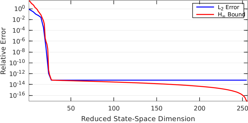
Figure 2: Model reduction error for the linear test system, see Section 6.1.

Fig. 2 shows the reduced order model’s relative $\operatorname{\mathcal{L}}_{2}$-norm model reduction error, as well as the upper bound for increasing reduced orders. The error evolves correctly tightly below the bound, until the numerical accuracy is reached.

6.2 Hyperbolic Evaluation

The second numerical example is given by a one-dimensional transport equation. An input-output system is constructed by selecting the left boundary as the input and the right boundary as the output:

$$\frac{\partial}{\partial t}z(x,t) =-\theta\frac{\partial}{\partial x},\quad x\in[0,1],$$

$$z(0,t) =u(t),$$

$$z(x,0) =0,$$

$$y(t) =z(1,t),$$

while the transport velocity $\theta\in[1.0,1.5]$ is treated as a parameter. This partial differential equation system is spatially discretized by a first-order finite-difference upwind scheme, yielding a SISO ordinary differential equation system:

$$\dot{x}(t) =A(\theta)x(t)+bu(t),$$

$$y(t) =cx(t),$$

with $A(\theta)=\theta A$. For this example, a spatial resolution of $\dim(x(t))=256$ is chosen, hence $A\in\operatorname{\mathbb{R}}^{256\times 256}$, $b\in\operatorname{\mathbb{R}}^{256}$ and $c\in\operatorname{\mathbb{R}}^{256}$. Since the system matrix is non-normal, using techniques such as POD may lead to unstable reduced order models. Thus, here a cross-Gramian-based balancing technique is used guaranteeing stability of the reduced model. For training, impulse responses for the extremal velocities are used; for testing, a Gauss bell input is utilized over ten uniformly random velocities, both utilizing the default integrator. The reduced order model quality is evaluated by the parametric norm [35]:

$$\|y(\theta)-\tilde{y}(\theta)\|_{\operatorname{\mathcal{L}}_{2}\otimes\operatorname{\mathcal{L}}_{2}} =\sqrt{\int_{\Theta}\|y(\theta)-\tilde{y}(\theta_{r})\|_{\operatorname{\mathcal{L}}_{2}}^{2}\operatorname{\mathrm{d}\!}\theta}.$$

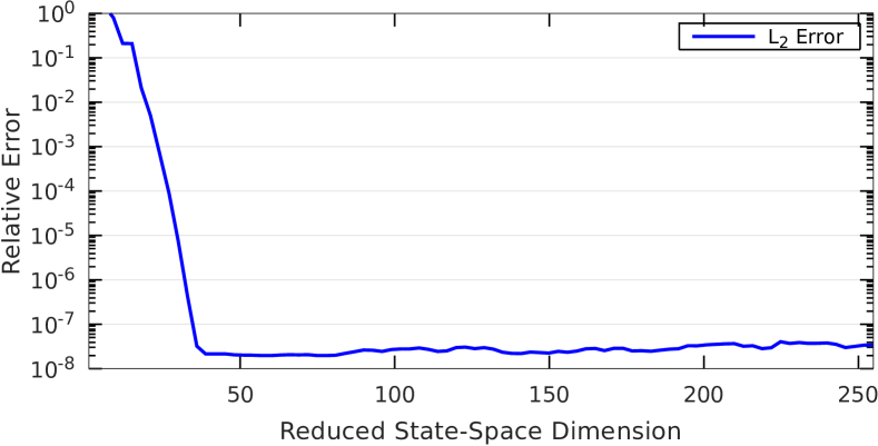
Figure 3: Model reduction error for the hyperbolic test system, see Section 6.2.

Even though the system is hyperbolic, a steep decay in error is obtained. Yet, due to the hyperbolicity and the parameter-dependence of the reduced order model, a lower overall numerical accuracy ($\approx 10^{-7}$) is achieved.

6.3 Nonlinear Validation

The third example involves a parametric nonlinear system, based on the hyperbolic network model [67],

$$\dot{x}(t) =A\tanh(K(\theta)x(t))+Bu(t),$$

$$y(t) =Cx(t).$$

The structure of this system is similar to the linear system model (2), yet the vector-field includes a hyperbolic tangent nonlinearity, in which the parametrized activation is described by a diagonal gain matrix $K(\theta)$, $K_{ii}=\theta_{i}$. A negative Lehmer matrix is selected as system matrix $A\in\operatorname{\mathbb{R}}^{256\times 256}$, a vector of sequential cosine evaluations as input matrix $B\in\operatorname{\mathbb{R}}^{256\times 1}$, a binary matrix $C^{4\times 256}$ as output matrix, and parameters $\theta\in\operatorname{\mathbb{R}}^{256}$ constrained to the interval $\theta_{i}\in[\frac{1}{2},1]$. For this system a combined state and parameter reduction is demonstrated. To this end an empirical non-symmetric joint Gramian is computed, using again an impulse input $u(t)=\delta(t)$, a zero initial state $x_{0,i}=0$ and the default integrator. The reduced order model quality is evaluated for the same input and initial state by the joint state and parameter norm $\|y(\theta)-\tilde{y}(\theta_{r})\|_{\operatorname{\mathcal{L}}_{2}\otimes\operatorname{\mathcal{L}}_{2}}$, with respect to the reduced parameters for ten uniformly random samples from the admissible parameter-space.

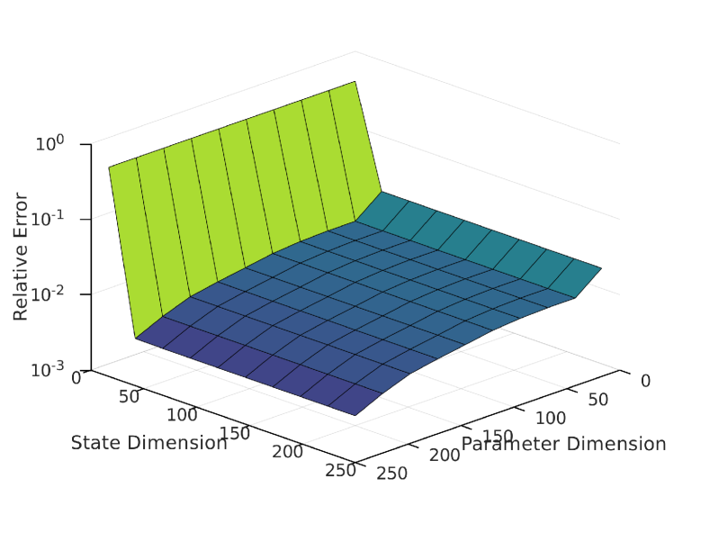
Figure 4: Model reduction error for the nonlinear test system, see Section 6.3.

Fig. 4 depicts the $\operatorname{\mathcal{L}}_{2}\otimes\operatorname{\mathcal{L}}_{2}$-norm model reduction error for increasing state- and parameter-space dimensions. The combined reduction errors decays for both, reduced state-space and reduced parameter-space, yet faster for the state-space. As for the parametric model, the numerical accuracy is reduced due to the combined reduction.

7 Concluding Remark

Empirical Gramians are a universal tool for nonlinear system and control theoretic applications with a simple, data-driven construction. The empirical Gramian framework - emgr implements empirical Gramian computation for system input-output coherence and parameter identifiability evaluation. Possible future extensions of emgr may include Koopman Gramians [91], empirical Riccati covariance matrices [9], or empirical differential balancing [51]. Finally, further examples and applications can be found at the emgr project website: http://gramian.de.

Code Availability

The source code of the presented numerical examples can be obtained from:

http://runmycode.org/companion/view/2077

and is authored by: Christian Himpe.

Acknowldgements

Supported by the German Federal Ministry for Economic Affairs and Energy, in the joint project: “MathEnergy – Mathematical Key Technologies for Evolving Energy Grids”, sub-project: Model Order Reduction (Grant number: 0324019B).

References

- [1] R. W. Aldhaheri. Model order reduction via real Schur-form decomposition. Internat. J. Control, 53(3):709–716, 1991. doi:10.1080/00207179108953642.
- [2] Y. M. Altman. Accelerating MATLAB Performance: 1001 tips to speed up MATLAB programs. CRC Press, 2015. URL: http://www.worldcat.org/search?q=bn%3A9781482211306.
- [3] A. C. Antoulas. Approximation of Large-Scale Dynamical Systems, volume 6 of Adv. Des. Control. SIAM Publications, Philadelphia, PA, 2005. doi:10.1137/1.9780898718713.
- [4] A. Barbagallo, V. F. De Felice, and K. K. Nagarajan. Reduced order modelling of a couette flow using balanced proper orthogonal decomposition. In 2nd Young ERCOFTAC Workshop, 2008. URL: http://dokumente.unibw.de/pub/bscw.cgi/2700941.
- [5] B. Basu. FreeMat. freemat.sourceforge.net.
- [6] U. Baur and P. Benner. Gramian-based model reduction for data-sparse systems. SIAM J. Sci. Comput., 31(1):776–798, 2008.
- [7] U. Baur, P. Benner, B. Haasdonk, C. Himpe, I. Martini, and M. Ohlberger. Comparison of methods for parametric model order reduction of time-dependent problems. In P. Benner, A. Cohen, M. Ohlberger, and K. Willcox, editors, Model Reduction and Approximation: Theory and Algorithms, pages 377–407. SIAM, 2017. doi:10.1137/1.9781611974829.ch9.
- [8] J. Bouvrie and B. Hamzi. Kernel methods for the approximation of nonlinear systems. SIAM J. Control Optim., 55(4):2460–2492, 2017. doi:10.1137/14096815X.
- [9] R. B. Choroszucha and J. Sun. Empirical Riccati covariance matrices for closed-loop model order reduction of nonlinear systems by balanced truncation. In Proceedings of the American Control Conference, pages Seattle, WA, USA, 3476–3482, 2017. IEEE. doi:10.23919/ACC.2017.7963484.
- [10] R. B. Choroszucha, J. Sun, and K. Butts. Nonlinear model order reduction for predictive control of the diesel engine airpath. In Proceedings of the American Control Conference, pages 5081–5086, Bosten, MA, USA, 2016. IEEE. doi:10.1109/ACC.2016.7526159.
- [11] M. Condon and R. Ivanov. Empirical balanced truncation of nonlinear systems. J. Nonlinear Sci., 14(5):405–414, 2004. doi:10.1007/s00332-004-0617-5.
- [12] M. Condon and R. Ivanov. Model reduction of nonlinear systems. Compel-Int. J. Comp. Math. Electr. Electron. Eng., 23(2):547–557, 2004. doi:10.1108/03321640410510730.
- [13] I. Dones, S. Skogestad, and H. A. Preisig. Application of balanced truncation to nonlinear systems. Ind. Eng. Chem. Res., 50(17):10093–10101, 2011. doi:10.1021/ie200706d.
- [14] J. W. Eaton, D. Bateman, S. Hauberg, and R. Wehbring. GNU Octave version 4.4.0 manual: a high-level interactive language for numerical computations, 2018. URL: http://www.gnu.org/software/octave/doc/interpreter.
- [15] C. Eberle and C. Ament. Identifiability and online estimation of diagnostic parameters with in the glucose insulin homeostasis. Biosystems, 107(3):135–141, 2012. doi:10.1016/j.biosystems.2011.11.003.
- [16] G. Fasshauer and M. McCourt. Kernel-based Approximation Methods using MATLAB, volume 19 of Interdisciplinary Mathematical Sciences. World Scientific, 2015.
- [17] K. V. Fernando. Covariance and Gramian Matrices in Control and Systems Theory. Ph.D. Thesis, University of Sheffield, 1982. URL: http://ethos.bl.uk/OrderDetails.do?uin=uk.bl.ethos.280627.
- [18] K. V. Fernando and H. Nicholson. On the Cauchy index of linear systems. IEEE Trans. Autom. Control, 28(2):222–224, 1983. doi:10.1109/TAC.1983.1103200.
- [19] K. V. Fernando and H. Nicholson. On the structure of balanced and other principal representations of SISO systems. IEEE Trans. Autom. Control, 28(2):228–231, 1983. doi:10.1109/TAC.1983.1103195.
- [20] K. V. Fernando and H. Nicholson. On the cross-Gramian for symmetric MIMO systems. IEEE Trans. Circuits Syst., 32(5):487–489, 1985. doi:10.1109/TCS.1985.1085737.
- [21] L. Fortuna and M. Fransca. Optimal and Robust Control: Advanced Topics with MATLAB. CRC Press, 2012. URL: worldcat.org/search?q=isbn%3A9781466501911.
- [22] J. Fu, C. Zhong, Y. Ding, J. Zhou, and C. Zhong. An information theoretic approach to model reduction based on frequency-domain cross-Gramian information. In Proceedings of the 8th World Congress on Intelligent Control and Automation, pages 3679–3683, Jinan, PRC, 2010. IEEE. doi:10.1109/WCICA.2010.5553913.
- [23] K. Fujimoto and J. M. A. Scherpen. On balanced truncation for symmetric nonlinear systems. In International Symposium on Mathematical Theory of Networks and Systems, volume 21, pages 1498–1502, 2014. URL: http://hdl.handle.net/11370/48dc6589-2b34-473a-9e4f-1f1a47b3a892.
- [24] J. S. Garcia and J. C. Basilio. Computation of reduced-order models of multivariable systems by balanced truncation. Int. J. Syst. Sci., 33(10):847–854, 2002. doi:10.1080/0020772021000017308.
- [25] D. Geffen, R. Findeisen, M. Schliemann, F. Allgöwer, and M. Guay. Observability based parameter identifiability for biochemical reaction networks. In Proc. Am. Control. Conf., pages 2130–2135, 2008. doi:10.1109/ACC.2008.4586807.
- [26] S. Gugercin, A. C. Antoulas, and C. Beattie. model reduction for large-scale linear dynamical systems. SIAM J. Matrix Anal. Appl., 30(2):609–638, 2008. doi:10.1137/060666123.
- [27] J. Hahn and T. F. Edgar. Reduction of nonlinear models using balancing of empirical Gramians and Galerkin projections. In Proc. Am. Control. Conf., volume 4, pages 2864–2868, 2000. doi:10.1109/ACC.2000.878734.
- [28] J. Hahn and T. F. Edgar. A gramian based approach to nonlinearity quantification and model classification. Ind. Eng. Chem. Res., 40(24):5724–5731, 2001. doi:10.1021/ie010155v.
- [29] J. Hahn and T. F. Edgar. Balancing approach to minimal realization and model reduction of stable nonlinear systems. Ind. Eng. Chem. Res., 41(9):2204–2212, 2002. doi:10.1021/ie0106175.
- [30] J. Hahn and T. F. Edgar. An improved method for nonlinear model reduction using balancing of empirical Gramians. Comput. Chem. Eng., 26(10):1379–1397, 2002. doi:10.1016/S0098-1354(02)00120-5.
- [31] J. Hahn, T. F. Edgar, and W. Marquardt. Controllability and observability covariance matrices for the analysis and order reduction of stable nonlinear systems. J. Process Control, 13(2):115–127, 2003. doi:10.1016/S0959-1524(02)00024-0.
- [32] J. Hahn, U. Kruger, and T. F. Edgar. Application of model reduction for model predictive control. In Proc. IFAC World Congress, volume 15(1), pages 632–637, 2002. doi:10.3182/20020721-6-ES-1901.00634.
- [33] B. Halvarsson, M. Castaño, and W. Birk. Uncertainty bounds for gramian-based interaction measures. In Latest Trends on Systems, volume 2, pages 393–398, 2010. URL: http://www.wseas.us/e-library/conferences/2010/Corfu/SYSTEMS/SYSTEMS2-07.pdf.
- [34] J. Hespanha. Linear Systems Theory. Princeton University Press, 2009. URL: http://www.ece.ucsb.edu/~hespanha/linearsystems/.
- [35] C. Himpe. Combined State and Parameter Reduction for Nonlinear Systems with an Application in Neuroscience. PhD thesis, Westfälische Wilhelms-Universität Münster, 2017. Sierke Verlag Göttingen, ISBN 9783868448818. doi:10.14626/9783868448818.
- [36] C. Himpe. emgr – EMpirical GRamian framework (version 5.4). http://gramian.de, 2018. doi:10.5281/zenodo.1241532.
- [37] C. Himpe, T. Leibner, and S. Rave. Hierarchical approximate proper orthogonal decomposition. arXiv e-prints 1607.05210, Cornell University, 2018. math.NA. URL: http://arxiv.org/abs/1607.05210.
- [38] C. Himpe, T. Leibner, S. Rave, and J. Saak. Fast low-rank empirical cross Gramians. Proc. Appl. Math. Mech., 17(1):841–842, 2017. doi:10.1002/pamm.201710388.
- [39] C. Himpe and M. Ohlberger. A unified software framework for empirical Gramians. J. Math., 2013:1–6, 2013. doi:10.1155/2013/365909.
- [40] C. Himpe and M. Ohlberger. Cross-Gramian based combined state and parameter reduction for large-scale control systems. Mathematical Problems in Engineering, 2014(Article ID 843869):1–13, 2014. doi:10.1155/2014/843869.
- [41] C. Himpe and M. Ohlberger. The empirical cross Gramian for parametrized nonlinear systems. IFAC-PapersOnLine (Proceedings of the 8th Vienna International Conference on Mathematical Modelling), 48(1):727–728, 2015. doi:10.1016/j.ifacol.2015.05.163.
- [42] C. Himpe and M. Ohlberger. A note on the cross Gramian for non-symmetric systems. Systems Science and Control Engineering, 4(1):199–208, 2016. doi:10.1080/21642583.2016.1215273.
- [43] C. Himpe and M. Ohlberger. Cross-Gramian-based model reduction: A comparison. In P. Benner, M. Ohlberger, A. Patera, G. Rozza, and K. Urban, editors, Model Reduction of Parametrized Systems, volume 17 of Modeling, Simulation and Applications, pages 271–283. Springer, Cham, 2017. doi:10.1007/978-3-319-58786-8_17.
- [44] V. Hrishikeshavan, J. S. Humbert, and I. Chopra. Gramian analysis of a shrouded rotor micro air vehicle in hover. Journal of Guidance, Control, and Dynamics, 37(5):1684–1690, 2014. doi:10.2514/1.G000066.
- [45] T. C. Ionescu, K. Fujimoto, and J. M. A. Scherpen. Singular value analysis of nonlinear symmetric systems. IEEE Trans. Autom. Control, 56(9):2073–2086, 2011. doi:10.1109/TAC.2011.2126630.
- [46] A. Jazlan, V. Sreeram, and R. Togneri. Cross Gramian based time interval model reduction. In Proceedings of the 5th Australien Control Conference (AUCC), pages 274–276, 2015. URL: http://ieeexplore.ieee.org/abstract/document/7361947/.
- [47] M. Jiang, J. Wu, L. Jiang, and X. Li. A Gramians based method for nonlinearity quantification of spatio-temporal systems. In Advanced Science and Technology Letters, volume 121, pages 38–42, Haikou, PRC, 2016. SERSC. doi:10.14257/astl.2016.121.08.
- [48] R. K. Johnson. The Elements of MATLAB Style. Cambridge University Press, 2011. doi:10.1017/CBO9780511842290.
- [49] I. Kalashnikova, M.F. Barone, S. Arunajatesan, and B.G. van Bloemen Waanders. Construction of energy-stable projection-based reduced order models. Applied Mathematics and Computation, 249:569–596, 2014. doi:10.1016/j.amc.2014.10.073.
- [50] R. E. Kalman. Mathematical description of linear dynamical systems. SIAM J. Control Optim., 1:182–192, 1963. doi:10.1137/0301010.
- [51] Y. Kawano and J. M. A. Scherpen. Empirical differential balancing for nonlinear systems. In Proceedings of the 20th IFAC World Congress, volume 50 of IFAC-PapersOnLine, pages 6326–6331, 2017. doi:10.1016/j.ifacol.2017.08.920.
- [52] A. Keil and J. L. Gouzé. Model reduction of modular systems using balancing methods. Technical report, Technische Universität München, 2003. URL: http://citeseerx.ist.psu.edu/viewdoc/summary?doi=10.1.1.485.2449.
- [53] D. I. Ketcheson. Highly efficient strong stability-preserving Runge-Kutta methods with low-storage implementations. SIAM J. Sci. Comput., 30(4):2113–2136, 2008. doi:10.1137/07070485X.
- [54] A. Krener and K. Ide. Measures of unobservability. In Proceedings of the 48th IEEE Conference on Decision and Control, 2009 held jointly with the 2009 28th Chinese Control Conference, pages 6401–6406, 2009. doi:10.1109/CDC.2009.5400067.
- [55] S. Lall, J. E. Marsden, and S. Glavaški. Empirical model reduction of controlled nonlinear systems. IFAC Proceedings Volumes (Proceedings of the 14th IFAC World Congress), 32(2):2598–2603, 1999. doi:10.1016/S1474-6670(17)56442-3.
- [56] D. Lawrence, J. H. Myatt, and R. C. Camphouse. On model reduction via empirical balanced truncation. In Proc. Am. Control Conf., volume 5, pages 3139–3144, 2005. doi:10.1109/ACC.2005.1470454.
- [57] C. E. Lieberman, K. Fidkowski, K. Willcox, and B. Van Bloemen Waanders. Hessian-based model reduction: large-scale inversion and prediction. Int. J. Numer. Methods Fluids, 71(2):135–150, 2013. doi:10.1002/fld.3650.
- [58] W. Q. Liu, V. Sreeram, and K. L. Teo. Model reduction for state-space symmetric systems. Syst. Control Lett., 34(4):209–215, 1998. doi:10.1016/S0167-6911(98)00024-3.
- [59] V. Lystianingrum, B. Hredzak, and V. G. Agelidis. Abnormal overheating detectability analysis based on cross Gramian for a supercapacitors string. In Power and Energy Society General Meeting, 2016. doi:10.1109/PESGM.2016.7741824.
- [60] X. Ma and J. A. De Abreu-Garcia. On the computation of reduced order models of nonlinear systems using balancing technique. In Proc. 27th IEEE Conf. Decis. Control, volume 2, pages 1165–1166, 1988. doi:10.1109/CDC.1988.194502.
- [61] The MathWorks, Inc., http://www.matlab.com. MATLAB.
- [62] B. Moaveni and A. Khaki-Sedigh. Input-output pairing based on cross-Gramian matrix. In International Joint Conference SICE-ICAS, pages 2378–2380, 2006. doi:10.1109/SICE.2006.314989.
- [63] B. C. Moore. Principal component analysis in linear systems: controllability, observability, and model reduction. IEEE Trans. Autom. Control, AC–26(1):17–32, 1981. doi:10.1109/TAC.1981.1102568.
- [64] P. N. Nikiforuk and M. M. Gupta. On stochastic perturbation theory for linear systems. In 1969 IEEE Symposium on Adaptive Processes (8th) Decision and Control, pages 5–c–1–5–c–2, 1969. doi:10.1109/SAP.1969.269923.
- [65] O. Nilsson and A. Rantzer. A novel approach to balanced truncation of nonlinear systems. In Proc. Europ. Control Conf., 2009. URL: http://ieeexplore.ieee.org/abstract/document/7074628/.
- [66] N. D. Powel and K. A. Morgansen. Empirical observability Gramian rank condition for weak observability of nonlinear systems with control. In 54th Annual Conference on Decision and Control, pages 6342–6348, 2015. doi:10.1109/CDC.2015.7403218.
- [67] Y. Quan, H. Zhang, and L. Cai. Modeling and control based on a new neural network model. In Proc. Am. Control. Conf., volume 3, pages 1928–1929, 2001. doi:10.1109/ACC.2001.946022.
- [68] P. Rogers, J. Marci, and S. Marinkovic. heterogeneous uniform memory access. In AMD, 2013. URL: http://events.csdn.net/AMD/130410%20-%20hUMA_v6.6_FINAL.PDF.
- [69] C. W. Rowley. Model reduction for fluids, using balanced proper orthogonal decomposition. Int. J. Bifurcat. Chaos, 15(3):997–1013, 2005. doi:10.1142/S0218127405012429.
- [70] M. B. Saltik, L. Özkan, S. Weiland, and P. M. J. Van den Hof. Sensor configuration problem: Application to a membrane separation unit. IFAC-PapersOnLine, 49(7):189–194, 2016. doi:10.1016/j.ifacol.2016.07.245.
- [71] G. Schelfhout and B. De Moor. Time-domain weighted balanced truncation. In 3rd European Control Conference, pages 1–4, 1995. URL: ftp://ftp.esat.kuleuven.ac.be/SISTA/schelfhout/reports/tbalred.ps.Z.
- [72] J. M. A. Scherpen. Balancing for nonlinear systems. Syst. Control Lett., 21(2):143–153, 1993. doi:10.1016/0167-6911(93)90117-O.
- [73] H. R. Shaker. Generalized cross-Gramian for linear systems. In Proc. IEEE Conf. Ind. Electron. Appl., pages 749–751, 2012. doi:10.1109/ICIEA.2012.6360824.
- [74] H. R. Shaker and M. Komareji. Control configuration selection for multivariable nonlinear systems. Ind. Eng. Chem. Res., 51(25):8583–8587, 2012. doi:10.1021/ie301137k.
- [75] H. R. Shaker and J. Stoustrup. An interaction measure for control configuration selection for multivariable bilinear systems. Nonlinear Dyn., 72(1):165–174, 2013. doi:10.1007/s11071-012-0700-z.
- [76] A. K. Singh and J. Hahn. Determining optimal sensor locations for state and parameter estimation for stable nonlinear systems. Ind. Eng. Chem. Res., 44(15):5645–5659, 2005. doi:10.1021/ie040212v.
- [77] A. K. Singh and J. Hahn. On the use of empirical Gramians for controllability and observability analysis. In Proc. Am. Control conf., volume 2005, pages 140–141, 2005. doi:10.1109/ACC.2005.1469922.
- [78] T. J. Snowden, P. H. van der Graaf, and M. J. Tindall. A combined model reduction algorithm for controlled biochemical systems. BMC Systems Biology, 11(1):1–18, 2017. doi:10.1186/s12918-017-0397-1.
- [79] D. C. Sorensen and A. C. Antoulas. The Sylvester equation and approximate balanced reduction. Numer. Lin. Alg. Appl., 351–352:671–700, 2002. doi:10.1016/S0024-3795(02)00283-5.
- [80] S. Streif, R. Findeisen, and E. Bullinger. Relating cross Gramians and sensitivity analysis in systems biology. Theory of Networks and Systems, 10.4:437–442, 2006. URL: http://hdl.handle.net/2268/130730.
- [81] T. H. Summers, F. L. Cortesi, and J. Lygeros. On submodularity and controllability in complex dynamical networks. IEEE Trans. Control Netw. Syst., PP(99):1–11, 2015. doi:10.1109/TCNS.2015.2453711.
- [82] C. Sun and J. Hahn. Model reduction in the presence of uncertainty in model parameters. J. Process Control, 16(6):645–649, 2006. doi:10.1016/j.jprocont.2005.10.001.
- [83] C. Sun and J. Hahn. Nonlinear model reduction routines for MATLAB. Technical report, Rensselaer Polytechnic Institute, 2006. URL: http://www.hahnresearchgroup.com/downloads/nonlinear-model-reduction-routines-matlab.
- [84] C. Sun and J. Hahn. Parameter reduction for stable dynamical systems based on Hankel singular values and sensitivity analysis. Chem. Eng. Sci., 61(16):5393–5403, 2006. doi:10.1016/j.ces.2006.04.027.
- [85] The MORwiki Community. MORwiki - Model Order Reduction Wiki. http://modelreduction.org.
- [86] The Octave Developers. GNU Octave. http://octave.org.
- [87] C. Tolks and C. Ament. Model order reduction of glucose-insulin homeostasis using empirical Gramians and balanced truncation. In IFAC PapersOnline, volume 50, pages 14735–14740, 2017. doi:10.1016/j.ifacol.2017.08.2576.
- [88] K. Willcox and J. Peraire. Balanced model reduction via the proper orthogonal decomposition. AIAA J., 40(11):2323–2330, 2002. doi:10.2514/2.1570.
- [89] M. Wu, B. Yin, A. Vosoughi, C. Studer, J. R. Cavallaro, and C. Dick. Approximate matrix inversion for high-throughput data detection in the large-scale MIMO uplink. In Proc. IEEE Int. Symp. Circ. Syst., pages 2155–2158, 2013. doi:10.1109/ISCAS.2013.6572301.
- [90] S. Yao, Y. Deng, and Z. Yu. Balanced truncation on empirical gramians for model-order-reduction of non-quasi-static effects in MOSFETs. In 9th International Conference on Solid-State and Integrated-Circuit Technology, pages 309–312, 2008. doi:10.1109/ICSICT.2008.4734525.
- [91] E. Yeung, Z. Liu, and N. O. Hodas. A Koopman operator approach for computing and balancing Gramians for discrete time nonlinear systems. arXiv e-print 1709.08712, Cornell University, 2017. cs.SY. URL: https://arxiv.org/abs/1709.08712.
- [92] M. Zhanfeng and H. Chao. Structure-preserving balanced truncation for flexible spacecraft using cross Gramian. Journal of Beijing University of Aeronautics and Astronautics, 34(12):1437–1440, 2008. URL: http://en.cnki.com.cn/Article_en/CJFDTOTAL-BJHK200812017.htm.