Non-Markovian quantum thermodynamics: laws & fluctuation theorems
Abstract
This work brings together thermodynamics and non-equilibrium quantum theory, by showing that a real-time diagrammatic technique on the Keldysh contour is an equivalent of stochastic thermodynamics for non-Markovian quantum machines (heat engines, refrigerators, etc). Symmetries are found between quantum trajectories and their time-reverses on the Keldysh contour, for any interacting quantum system coupled to ideal reservoirs of electrons, phonons or photons. These lead to quantum fluctuation theorems the same as the well-known classical ones (Jarzynski and Crooks equalities, integral fluctuation theorem, etc), whether the system’s dynamics are Markovian or not. Some of these are also shown to hold for non-factorizable initial states. The sequential tunnelling approximation and the cotunnelling approximation are both shown to respect the symmetries that ensure the fluctuation theorems. For all initial states, energy conservation ensures that the first law of thermodynamics holds on average, while the above symmetries ensures that the second law of thermodynamics holds on average, even if fluctuations violate it. [ERRATUM added: March 2021]
pacs:
73.63.-b, 05.30.-d, 05.70.Ln, 05.10.Gg, 72.15.Jf, 84.60.Rb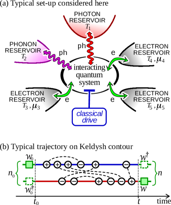
ERRATUM (14 March 2021). The published version of this article contained a stupid error in the condition for the validity of the Crooks equaton. This error is corrected here by the red text in section VIII.4.
I Introduction
The laws of thermodynamics were derived for macroscopic machines, where entropy-reducing fluctuations (e.g. a gas spontaneously drifting into one corner of its container) are so rare that they have been referred to as thermodynamic miracles. Thermdynamic-Miracles In microscopic systems on short timescales, these “miracles” are rather common, and we now know they obey fluctuation theorems.Derrida-CRAS2007 ; Searles-Review-2008 ; Campisi-review2011 ; qu-thermo-review-Anders ; qu-thermo-review-Millen There is a unifying theory of such theorems in classical systems called stochastic thermodynamics,Seifert-PRL2005 ; Schmiedl-Seifert2007 reviewed in Refs. [Seifert-review2012, ; van-Broeck-review2015, ; Seifert-PRL2016, ; our-review-2017, ]. It gives the Jarzynski Jarzynski , Evans-Searles Evans-Searles1994 and Crooks Crooks1999 ; Tasaki equalities in the relevant limits. It was used to show Seifert-PRL2005 ; Schmiedl-Seifert2007 that any classical system with Markovian dynamics obeys
| (1) |
where is the total entropy change of the system and reservoirs,footnote:definitionS and the average is over all possible thermal fluctuations.Footnote:units This has become known as the integral fluctuation theorem,Seifert-PRL2005 ; Schmiedl-Seifert2007 ; Seifert-review2012 ; van-Broeck-review2015 even if a similar identity had appeared under the name non-equilibrium partition identity earlier.Yamada-Kawasaki1967 ; Morriss1985 ; Carberry2005 Eq. (1) tells us that the second law of thermodynamics is obeyed on average, . Yet Eq. (1) also tells us that fluctuations with must occur (even if rarely), otherwise would be less than one.
At the same time, there is great interest in the thermodynamics of nanoscale machines, particularly those which convert heat into electricity, or use electricity to perform refrigeration. Such machines are definitely not macroscopic, so we can expect them to exhibit fluctuations similar to those described above. However most of them also exhibit quantum effects that are not captured by classical theory of stochastic thermodynamics. Many operate in the steady-state, such as the quantum-dot heat-engines experimentally realized in Refs. Roche15 ; Hartmann15 ; Thierschmann15 , or other mesoscopic systems which exhibit thermoelectric effects our-review-2017 ; CRAS , while others involve pumping cycles Juergens2013 . The general case of such a machine is sketched in Fig. 1a.
This work shows that a diagrammatic technique on the Keldysh contour — real-time transport theory Schoeller-Schon1994 ; Konig96 ; Konig97 ; Schoeller-review1997 — provides an equivalent of stochastic thermodynamics for any quantum system coupled to reservoirs (Fig. 1a) whether that system’s dynamics are Markovian or not. It makes the connection between the contribution of a double-trajectory, , on the Keldysh contour and the contribution of its time-reverse, (Fig. 5a). This is enough to show that such systems respect the same fluctuation theorems as classical Markovian systems, and so obey the second law of thermodynamics on average. For the second law, our proof goes beyond those for Markovian quantum systems Kosloff-review2013 , those for systems with mean-field interactions,Nenciu2007 ; 2012w-2ndlaw and Keldysh treatments for non-interacting systems (quadratic Hamiltonians) Sanchez-2ndlaw2014 ; Esposito-2ndlaw ; Bruch-2016 or adiabatic driving Sanchez-2ndlaw-2016 based on the Keldysh techniques reviewed in Ref. [Kamenev-book, ]. This connection between fluctuation theorems Campisi-review2011 ; qu-thermo-review-Anders ; qu-thermo-review-Millen and a non-equilibrium quantum theory for transport through interacting systems,Schoeller-Schon1994 ; Konig96 ; Konig97 ; Schoeller-review1997 ; Leijnse2008 ; Schoeller2009 ; Wegewijs2014 ; Sothmann2014 ; Schulenborg2016 provides a powerful tool for modelling energy production and refrigeration at the nanoscale. In this context, significant currents and power outputs require significant system-reservoir coupling. However, only systems in the weak coupling limit have Markovian dynamics,Davies74 ; Davies76 . Thus there is great interest in improving the power output of experimental set-ups like the quantum dot heat-engines in Refs. Roche15 ; Hartmann15 ; Thierschmann15 by taking them to stronger coupling, where their dynamics will be non-Markovian systems.
Previous proofs of fluctuation theorems in non-Markovian quantum systems exist,Campisi-review2011 but rely on treating the system and reservoirs together as a single isolated quantum system. This is elegant, but is not amenable to calculating a given machine’s power or efficiency, except in the rare cases where the full Hamiltonian (system plus reservoirs) is exactly soluble. It gives no indication of what approximations allow calculations of this power or efficiency, without an unphysical violation of fluctuation theorems and of the second law of thermodynamics. This work finds a microscopic symmetry which underlies the fluctuation theorems, beyond the Markovian quantum systems considered in Ref. [Maxime+Alexia2016, ]. This enables one to identify a family of approximations that allow tractable calculations of machine power and efficiency, with no risk of violating the second law or fluctuation theorems.
I.1 Overview of this work
The central observation of this work is the result connecting trajectories on the Keldysh contour in a system, to time-reversed trajectories in a time-reversed system, given in section VII.5 and shown schematically in Fig. 5. The sections leading up to section VII set the scene, with section VI making the observation that such trajectories obey the first law of thermodynamics on average. Then section VII itself provides a derivation of the result connecting trajectories to their time-reverse.
The rest of this work then uses this result in deriving various fluctuation theorems. Section VIII uses it to derive various fluctuation theorems in various situations, such as the Jarzynski equality and the Crooks equation. In particular, it shows that the integral fluctuation theorem in Eq. (1) holds for any system which starts in a product state with the reservoirs, thereby showing that any such system obeys the second law of thermodynamics on average. Section IX provides similar proofs for situations where the system and reservoir start in a non-factorizable initial state. Finally, section X discusses approximations that respect the result in section VII.5, and thereby will not violate any of the fluctuation theorems in sections VIII and IX, and so will always satisfy the second law of thermodynamics on average.
I.2 A comment on the system-reservoir coupling
The recent literature on Keldysh for quantum thermodynamics Sanchez-2ndlaw2014 ; Esposito-2ndlaw ; Bruch-2016 ; Sanchez-2ndlaw-2016 has strongly debated the role of the average energy stored in the system-reservoir coupling, , in models of adiabatic pumping or in which interactions are absent. The initial claim was that should be separated into two equal parts, with one part being assigned to system and the other part to the reservoir, however Ref. [Bruch-2016, ] argued that this was mainly a matter of calculational convenience.
In light of this debate, it is worth mentioning the role of in the diagrammatic approach used here, whose differences from the approach in Refs. [Sanchez-2ndlaw2014, ; Esposito-2ndlaw, ; Bruch-2016, ; Sanchez-2ndlaw-2016, ], are described in section II below. Firstly, appears in the first law, but does not appear in the second law or the integral fluctuation theorem, since they involve entropy rather than energy. Secondly, it is not convenient to assign any part of to the reservoirs for the following reason. In the cases considered here, each reservoir is in a state that is “simple”, that is to say it is in local equilibrium, which is completely described by two parameters; temperature and electrochemical potential. However, the system state is not “simple” in this sense, because it is typically far from equilibrium (due to the action of multiple reservoirs and/or driving), and requires more than just these two parameters to describe it. This means that the system-reservoir coupling is also not “simple”. Hence, it is unhelpful to associate any part of the system-reservoir coupling with the reservoir state, because one then loses the simplicity of the latter. In contrast the energy in the system-reservoir coupling always appears together with the system energy (see section VI), and as neither contribution is “simple” in the above sense, there is no disadvantage with making the choice to combine the two into a single effective internal system energy. That said, this article keeps the energy in the system-reservoir coupling separate from the system energy throughout, to avoid ambiguity.
II Hamiltonian
This work considers a small quantum system with the Hamiltonian, , which may include a time-dependent driving and interactions between the particles in the system. This system (shown at the centre of Fig. 1a) acts as a machine changing the heat and work in the reservoirs that surround it. Each term in contains one creation operator for a system electronic state, , for every annihilation operator, . This system is coupled to multiple reservoirs of non-interacting fermions (electrons) via couplings , or non-interacting bosons (photons or phonons) via couplings . This article uses the word “set-up” to refer to the system and reservoirs together; the total Hamiltonian of this set-up is
| (2) | |||||
The sums are over electron (el) and photon/phonon (ph) reservoirs. For el reservoirs,
| (3) |
for reservoir ’s state with energy, creation and annihilation operators , and . The tunnel coupling,
| (4) |
where and contain only system operators, and may be time-dependent. The change in the system state when an electron is added from reservoir ’s state is given by . The reverse process is given by . The simplest case has , however if the coupling depends on the system state, then contains extra factors of . For bosonic reservoirs, one replaces the fermionic operators and by bosonic ones. The simplest case has , meaning the system goes from to when a boson is absorbed from reservoir ’s state .
The first step to using the real-time transport theorySchoeller-Schon1994 ; Konig96 ; Konig97 ; Schoeller-review1997 is to write all system operators as matrices acting on the basis of many-body system states, see e.g. appendix C of Ref. [our-review-2017, ]. We go to an interaction representation (indicated by calligraphic symbols), where system operators evolve under a matrix
| (5) |
with indicating time-ordering. Hence,
| (6) |
Reservoir operators evolve under , so we have
| (7) |
The initial condition (at time ) is an arbitrary system state in a product state with the reservoirs. Each reservoir is in its local equilibrium with temperature and chemical potential ( for reservoirs of photons or phonons). We treat exactly, and keep the reservoir’s effect on the system finite, in the limit of vanishing reservoir level-spacing. This requires taking the system’s coupling to each reservoir mode to zero, as the density of such modes goes to infinity, so this coupling can be treated at lowest-order (second-order).Caldiera-Leggett-1983a ; Caldiera-Leggett-1983b ; Leggett-et-al ; Schoeller-review1997 None the less, the system may interact with any number reservoir modes at one time (all orders of cotunnelling events), and these interactions do not commute. Upon tracing out the reservoirs, the resulting system dynamics are highly non-Markovian. Thus its dynamics are not described by Markovian master equations (Lindblad equations), whose thermodynamics have already been well studied.Kosloff-review2013 Thess dynamics are represented in terms of a Keldysh double-trajectory, as in Fig. 1b, where each second-order interaction with a given reservoir mode is represented by a pair of interactions joined by a dashed line.
For readers familiar with the Keldysh methods reviewed in Kamenev’s textbook Kamenev-book and used in Refs. [Sanchez-2ndlaw2014, ; Esposito-2ndlaw, ; Bruch-2016, ; Sanchez-2ndlaw-2016, ], we note that the method used here is different at the level of what is treated as a perturbation. In Kamevev’s textbook, the Hamiltonian is written in the single particle basis; in this basis the Hamiltonian is quadratic in the absence of interactions between particles, and so is exactly soluble. One then uses increasingly sophisticated perturbative techniques to include the interaction terms such as electron-electron interactions (which are quartic in the single-particle operators). In contrast, this work uses a diagrammatic method on the Keldysh contour referred to as the real-time transport theorySchoeller-Schon1994 ; Konig96 ; Konig97 ; Schoeller-review1997 , which takes a different starting point; it starts in the many-body basis for the system Hamiltonian (the fact that it is in real time is not particularly important). In this basis, the physics of the system alone is trivial (including all interaction effects); however the system-reservoir couplings take forms that are too complicated to treat exactly. Thus, one has moved the difficulty from the interaction terms to the system-reservoir coupling terms. This is why this coupling must be treated as a perturbation, for which one sums up classes of irreducible diagrams within some suitable approximation scheme.
III Assumption of no Maxwell demons in reservoirs
The equations of classical and quantum physics are reversible. For example, if all degrees of freedom in a quantum system were easy to observe and extract work from, the fact that the full wavefunction of the system and reservoirs undergoes unitary evolution means no (von Neumann) entropy is ever produced. In both classical and quantum physics, entropy production emerges from a physically motivated assumption about which degrees of freedom are easy to observe and extract work from, and which are not. Typically this assumption separates everything into macroscopic and microscopic dynamics, where macroscopic dynamics are easy to observe and extract work from, while the microscopic dynamics are inaccessible. All works on thermodynamics make some sort of assumption of this type, explicitly or implicitly.
The assumption at the basis of this work is presented here, for compactness it is referred to as the “assumption of no Maxwell demons in reservoirs”. It requires that the system operates without knowing microscopic details of the reservoirs, beyond those encoded in the system-reservoir interaction in Eq. (2). For example, this disallows Maxwell’s “observant and neat-fingered” demons Maxwell (which are usually just circuitry built by physicists) which measure individual reservoir states, and then feedback this information by making a change in the time-dependence of or in Eq. (2) which is conditional on the result of the measurement. Just as in classical mechanics, assuming no Maxwell demons is crucial in the emergence of the second law from the underlying theory. This assumption makes all classical correlations and quantum entanglement between system and reservoirs at the end of the evolution irrelevant, since the system cannot extract work from them. Hence, one can trace out the reservoirs when calculating system entropy, and vice versa. Further, even though the system pushes certain reservoir modes out of equilibrium, it is assumed that this information is inaccessible, so no more work can be extracted from the reservoir than if it were in a thermal state with the same energy.
Superficially, one might thing this work has nothing to say about experimental implementations of Maxwell demons in quantum systems, similar to Refs. [Pekola-Demon, ; Cottet-Demon, ]. However, in those cases where the demon is completely mechanical (made of some finite number of degrees of freedom coupled to reservoirs with or without time-dependent driving), we can include these degrees of freedom in the system Hamiltonian , and all results in this work apply.
IV Trajectories
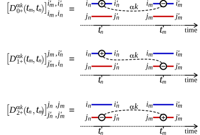
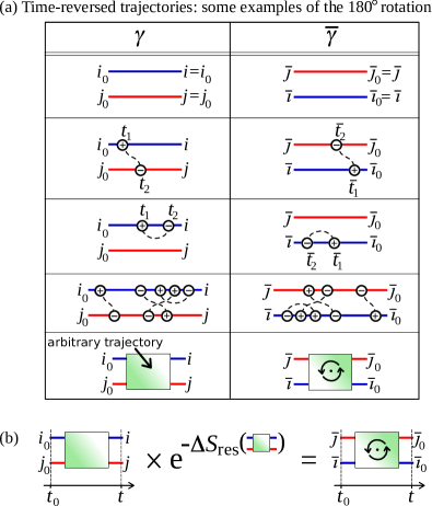
Consider a trajectory on the Keldysh contour, whose upper-line goes from system’s many-body state at time to at time , and whose lower line goes from to (see examples in Fig. 5a). Matrix elements for transitions are time ordered on the upper line and reverse-time ordered on the lower line. Each transition (each dashed-line in ) has a weight determined by whether it is , or in Fig. 2 (see below). Real transitions correspond to in Fig. 2 and virtual transitions to and . The trajectory’s weight, , is the product of all of these factors of , multiplied by a factor of for each crossing of dashed-lines.Schoeller-review1997 The probability to go from one system state to another in time , is simply the sum of the weights of all trajectories between those states.
The dashed-lines have the following weights,
| (8) | |||||
| (9) | |||||
| (10) |
where and . The factor is the number of particles in state of reservoir ; it is with for fermionic reservoirs and for bosonic reservoirs. Here,Footnote:units
| (11) |
which is the entropy change of reservoir when a particle is added to state . Identifying Eq. (11) with an entropy change follows from the Claussius definition of entropy, applicable here because each reservoir is in its own local thermodynamics equilibrium with a well defined temperature.
The weight of (for ) is given by the Hermitian conjugate of (so and ) with replaced by . Hence
| (12) | |||||
| (13) | |||||
| (14) |
Here is the number of ways one can add a particle to state of reservoir . For any reservoir (fermionic, bosonic or other) in internal equilibrium,
| (15) |
which is know as local detailed balance or micro-reversibility. For fermion or boson distributions, this is guaranteed by the fact that with for fermions, and for bosons. Physically, removes a particle from the system and adds it to state of reservoir ; this adds a work of and heat of to reservoir . Thus, involves a change of reservoir ’s entropy of in Eq. (11). The reverse process, , removes such a particle from reservoir , changing the reservoir’s entropy by . Contributions and do not change the number of particles in the reservoirs, and so involve no reservoir entropy change.
V Total Entropy
The assumption of no Maxwell demons in the reservoirs implies that entanglement between system and reservoir cannot be used to produce work. Then the correct definition of the total entropy production, , is the sum of that for the system (sys) and reservoirs (res),
| (16) |
with no term related to system-reservoir entanglement. We take the change in entropy of each reservoir to be given by the Claussius formula. This means that the change in reservoir ’s entropy, , for a trajectory is taken to be the sum of the entropy changes associated with each of the transitions in .
As the system is typically in a highly non-equilibrium state, one cannot use the Claussius law to calculate its entropy. In the stochastic thermodynamics of classical systems,Schmiedl-Seifert2007 ; van-Broeck-review2015 ; our-review-sect8.10 an entropy is assigned to each system state in such a way that the entropy of the system averaged over all such system states is the Shannon entropy. For quantum systems, one can do exactly the same thing, if (and only if) the system’s density matrix is in its diagonal basis. To get this entropy for the system’s initial density matrix (at time ), we write it as
| (17) |
where is the unitary matrix which rotates the system density matrix at time to its diagonal basis. This means that is the probability to find the system in state of its diagonal basis. In this basis, the system’s von Neumann entropy, is simply , where the sum is over the elements of the diagonal density matrix. Thus, one can treat each element in the sum as a contribution to the entropy from a given initial state, so that state ’s contribution to the entropy of the initial system state is,
| (18) |
with the average over all (i.e. a sum over weighted by the probability of state ) giving the system’s initial von Neumann entropy. The final system state’s entropy (at time ) is calculated in the same way by rotating to the diagonal-basis of the final system density matrix, given by for unitary , and assigning to the state an entropy of
| (19) |
with being the probability that the system is in state of the diagonal basis of its reduced density matrix at time . Eqs. (18.19) can be used to associate trajectory , from initial state to final state , with an entropy change in the system of
| (20) |
as in the stochastic thermodynamics of classical rate equations. Recall that this is only possible because the trajectory is defined as going from a system-state in the diagonal basis of the system density matrix at time , to a system-state in the diagonal basis of the system’s final density matrix (which is found by tracing out the reservoirs at the end of the evolution). This requires calculating the final density matrix (and finding its diagonal basis); this is much like in usual stochastic thermodynamics, where one also needs a complete knowledge of the final state probability distribution to assign entropies to it.
VI First law of thermodynamics
Here we show that energy conservation ensures that the first law of thermodynamics is obeyed on average. If one goes beyond the average, there are fluctuations that violate the first law, much like the fluctuations that violate the second law. These are little studied to-date, and merit a detailed study of their own. In this section, we restrict ourselves to considering the average energy in the set-up, and thereby show that the first law holds on average.
To ensure energy conservation, one must sum the three terms which contribute to the total energy; the energy in the reservoirs, the energy in the system, and the energy in the system-reservoir coupling. If the system is not driven this total energy is conserved. If the system is driven then the difference between the final and initial total energy is the work done by the drive, thus for between time and time , the average work done by the drive is
| (21) | |||||
where is the energy change in the reservoirs, is the energy change in the system, and is the energy change in the system-reservoir coupling.
Of course, all terms in this sum are necessary to get to get energy conservation, irrespective of whether one can physically measure each of them or not. Under the assumption of no Maxwell demons in the reservoirs, made in section III, one can measure the energy in the system and reservoirs, but not that in the system-environment coupling, since that depends on the state of individual reservoir modes. In such a case, one could none the less determine by using Eq. (21), assuming one can also measure the work done by the drive, .
The average energy in the quantum system is
| (22) |
while that in the system-reservoir coupling is
| (23) | |||||
where the trace in is over the system states and is the reduced system density matrix, but contains traces over the total density matrix (including reservoirs).
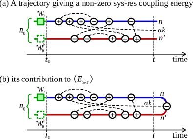
The trajectories which sum to give the average change in the system energy, , are those considered elsewhere in this article, such as those in Fig. 1b or Fig. 5. However, the trajectories which sum to give the average change in the energy in the system-reservoir coupling, , are rather different from those considered elsewhere in this article. They have an additional single interaction vertex with mode of reservoir at some time before , so that at time the system is in a superposition of a state with different numbers of particles in reservoir (see Fig. 3). Luckily, they have exactly the same structure as those used to calculate the current into the system in Refs. Schoeller-Schon1994 ; Konig96 ; Konig97 ; Schoeller-review1997 ; currents are given the difference between the term that creates a particle in the reservoir and one that destroys a particle, while the energy in the system-reservoir coupling is given by the sum of these two terms. These trajectories are not discussed further here, because Ref. [Schoeller-Schon1994, ; Konig96, ; Konig97, ; Schoeller-review1997, ] go into great detail about how to calculate their contribution.
The fact that reservoir is in local thermodynamic equilibrium defined by its temperature and electrochemical potential , mean it makes sense to split its energy, , into two contributions
| (24) |
with
| (25) | |||||
| (26) |
Then the change in reservoir energy between time and can be defined as
| (27) |
the first quantity here is the average work done by the reservoir , and the second quantity is the average heat flow out of the reservoir . There is no ambiguity in this separation, because the fact the reservoir is in local equilibrium means that the former (the work done) has no entropy change associated with it, while the latter (the heat change) is associated with an entropy change of
| (28) |
The trajectories which sum to give these average changes in a reservoir’s energy are those considered elsewhere in this article, such as those shown in Fig. 1b or Fig. 5. However the change in work or heat in the reservoir is extremely easy to read from a given trajectory, one simply sums up the change in work or heat for each dashed line symbolizing , as outlined at the end of section IV.
Given these definitions and Eq. (21), one easily arrives at the first law of thermodynamics for the average dynamics of the set-up;
| (29) | |||||
where we define as the total work done on the system by drive or reservoirs,
| (30) |
It thereby seems natural to interprete as the change in the effective internal energy of the system (an effective energy which includes the system-reservoir coupling), as mentioned in section I.2.
Just as in classical thermodynamics systems, the simplest cases to consider are those where the system returns to its initial state at the end of the evolution, so that its internal energy is the same at the final time, , as it was at the initial time, . Then , which means that Eq. (29) directly gives the simplest and best-known consequence of the first law; the work output of the machine equals the heat absorbed from the reservoirs.
Note that the change of energy in the reservoirs was separated into a change of heat and a change of work, but this was not done for the energy of the system or the system-reservoir coupling. The reason is that each reservoir is in local thermodynamic equilibrium, with a well-defined temperature, when the system and system-reservoir couplings are typically far from equilibrium with no well-defined temperature. Thus there is no ambiguity in the separation of energy into heat and work in a reservoir, see Eq. (28), but there is no simple way to make the same separation for the system or for the system-reservoir couplings.
VII Time-reversed set-up
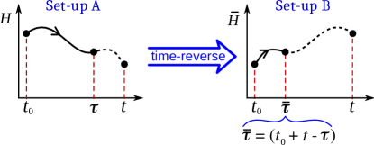
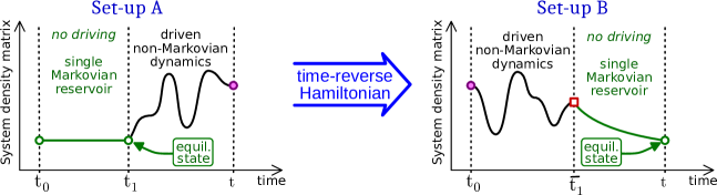
As in classical systems, one derives fluctuation theorems by comparing two different set-ups (A and B), where the Hamiltonian in set-up B is the time-reverse of the Hamiltonian in set-up A over the time-window from to . To be clear, whatever the Hamiltonian of set-up A, we can invent a set-up B whose Hamiltonian is the time-reverse of set-up A. In the special case of a time-independent Hamiltonian without external magnetic fields or spins, the two set-ups are identical, but otherwise they are not.
The objective of this section is to make the connection between weight of trajectories on the Keldysh contour in set-up B and set-up A. This starts by making the connection between the terms in the Hamiltonians of set-ups A and B in section VII.1, and then between the perturbative terms in the interaction representation in section VII.3. This enables one to make the connection between the weight of individual transitions in section VII.4, from which one gets the connection between weight of trajectories on the Keldysh contour in set-up B and set-up A in section VII.5. The central observation of this work is this relationship, given in Eq. (48) below. It is this relationship which is so similar to the relationship between trajectories in the stochastic thermodynamics theory for classical Markovian systems,Schmiedl-Seifert2007 ; van-Broeck-review2015 ; our-review-sect8.10 that we can use very similar logic to derive various well-known fluctuation theorems in section VIII.
VII.1 Time-reversed Hamiltonian
If A’s Hamiltonian (system+reservoir) is in Eq. (2), then B’s is , where is the time-reverse operator in Messiah’s texbook.Messiah-chapt15 The main results we need from Messiah’s texbook are recalled here in Appendix A, with the most trivial case sketched in Fig. 4. Thus if set-up A has a given time-dependent system Hamiltonian, , with given system-reservoir couplings, , then set-up B is chosen to have the system Hamiltonian and system-reservoir couplings
| (31) | |||||
| (32) |
where the bar above a symbol means that it is in set-up B, while the bar’s absence means in it is in set-up A.
These equations are cast in terms of matrix elements by inserting them between and , then
| (33) | |||||
| (34) |
where . Thus the matrix elements for transitions from system state to system state in set-up B (whose Hamiltonian is the time-reverse of set-up A’s), are the same as the matrix elements from system state to system state in set-up A. Spinless systems written in a basis of position states are trivial, because then . However, if one is working with basis states with non-zero momentum states, then is the state with the opposite momentum from . If one is working with spins, then the state is the state with the opposite spin from from state .
Equally, the reservoir Hamiltonians for set-up B are the time-reverse of those in set-up A, so reservoir in set up B has a Hamiltonian
| (35) |
where is that reservoir’s Hamiltonian in set-up A. In the absence of spins or external magnetic fields, this time-reverse operation is of no consequence. However, if reservoir in set-up A is a reservoir of electrons which are spin-up with respect to some axis, then the same reservoir in set-up B will contain electrons which are spin-down with respect to that axis. Similarly, if there is an external magnetic field acting on the reservoir in set-up A, then the field must be reversed in that reservoir in set-up B. For photon or phonon reservoirs, the relation between their Hamiltonians in the two set-ups is the same as in Eq. (35).
VII.2 Reservoir states are not time-reversed
If one evolves an initial state under a Hamiltonian, time-reverses the state, and evolves it under the time-reversed Hamiltonian, the dynamics in the second part of the evolution will look like a time reverse of the dynamics in the first part of the evolution.
However, this work’s set-up A and set-up B are a different time-reversal situation, in which each set-up is divided into a system and reservoirs, and we make the “assumption of no Maxwell demons in the reservoirs” in section III. This assumes the set-up and its drive are not aware of the microscopic dynamics of the reservoirs, as such one cannot time-reverse the state of the individual modes in the reservoirs, even if one can can time-reverse the reservoirs’ Hamiltonians (typically time-reversing the reservoir part of the Hamiltonian only requires interchanging the chemical potentials on spin-up and spin-down reservoirs and reversing any external magnetic fields acting on the reservoirs). Thus, even if we time-reverses the system state and time-reverses the total Hamiltonian, we will not see time-reversed dynamics, because we have not time-reversed the reservoir states.
Suppose set-up A starts with the system and reservoirs in a produce state, and then evolves. The system becomes correlated and/or entangled with individual reservoir modes. A measurement of the system state indicates that it is decohering and decaying towards a thermal state. A measurement of individual reservoir modes shows that an infinitesimal proportion of them are acquiring a non-thermal state. Then in set-up B, the total Hamiltonian is the time-reverse of that is set-up A, and the initial state is a product state, where the system state is the time reverse of the final system state in set-up A, and the reservoir modes are taken to be thermal (i.e. not time-reversed). The system state in set-up B does not become less correlated and/or entangled with the reservoirs as it evolves (as it would if we had time-reversed the full state, including the reservoir modes). Instead, the system continues to become more entangled with reservoir modes, which means that a measurement of the system state in set-up B will indicate that it also decoheres and decays towards a thermal state.
VII.3 Time-reversal for the interaction representation
Under time-reversal, the matrix representation of the system evolution operator is
| (36) |
Now, to simplify the algebra, it is assumed that a complete solution of the dynamics under exists, then the final state of the system (its state at given time ) can always be written in a basis chosen such that . Then, the unitary of means that
| (37) |
Given this one has
| (38) |
The interaction between the system and the reservoirs at time is written in the interaction representation for the time-reversed Hamiltonian as
| (39) |
where the matrix is defined above. Substituting in Eqs. (32,38) on the right, and comparing with Eq. (6), one finds that
| (40) |
for all between and .
For what follows it is convenient to cast this equality in terms of matrix elements by inserting it between and , then
| (41) |
Thus the matrix element for reservoir-induced transitions from system state to system state in set-up B (the set-up whose Hamiltonian is the time-reverse of set-up A’s), is the same as the matrix element from system state to system state in set-up A.
VII.4 Time-reversal symmetry between -transitions
Eq. (9) implies that the transition in the time-reserved system (set-up B) must have the weight
| (42) | |||||
where . Now substituting in Eq. (41), and noting that , we get
| (43) | |||||
Now comparing this with in Eq. (13), one sees the only difference is the factors of . However, local detailed balance in reservoir implies Eq. (15), so
| (44) |
Exactly the same logic holds if one starts with in place of . One just has to take the Hermitian conjugate throughout (so and ) and replace by , getting the results in Eq. (47a).
Similarly, Eq. (8) means that
| (45) | |||||
note that , since it is assumed that . As above, Eq. (41) is substituted in, and one notes that , to get
| (46) | |||||
which is the same as the right hand side of Eq. (10). One can do the same for .
The result of all these relations between s in the time-reversed set-up (set-up B) and the original set-up (set-up A) can be summarized as follows
| (47a) | |||||
| (47b) | |||||
where .
VII.5 Time-reversed trajectories
For any trajectory, , on the Keldysh contour in set-up A, one can define a trajectory in set-up B which is the time-reverse of . More precisely, is defined by rotating by in the plane of the page, and replacing all states by their time reverse, see Fig. 5a. The time-reverse of state is .
One then observes that if contains a -factor on the right hand side of one of the equality in Eq. (47), then then contains the -factor on the left hand side of the same equality, and vice-versa. The weights of trajectory in set-up A and in set-up B are given by products of the factors of that form each of them, this results in the central observation of this work (shown graphically in Fig. 5b),
| (48) |
where is the weight of double-trajectory in set-up A, and is that of in set-up B. The reservoir entropy change, , is the sum of the for all transitions in .
Now consider a double-trajectory, , which goes from the th state in the diagonal basis of to the th state in the diagonal basis of (see Fig. 1b). The subscript “d” is to indicate that it goes from diagonal basis to diagonal basis. Let us define its weight as , this equals multiplied by a factor of to transformation out of the diagonal basis at time , and a factor of to go to the diagonal basis at time . The unitarity of the transformations and means they do not change or , so one has
| (49) |
Here, one must recall that the trajectory is in set-up A, and goes from the state in the diagonal basis of the (initial) system density matrix at time , to the state in the diagonal basis of the (final) system’s reduced density matrix at time . Its time-reverse trajectory is a trajectory in set-up B which goes from state at time to state at time .
This relation is much the same as in Markovian stochastic thermodynamics of classical systems and which was used to derive various of the best known fluctuation theorems.Schmiedl-Seifert2007 ; van-Broeck-review2015 ; our-review-sect8.10 In the next section, we will show that a very similar procedure allows us to derive these fluctuation theorems for quantum systems with non-Markovian dynamics. In particular, we will show that the integral fluctuation theorem in Eq. (1) holds for any system, which we will show implies that any system will satisfy the second law of thermodynamics on average, .
However, a complication in these quantum system (absent in the classical ones) is the question of the basis in which the dynamics are diagonal. It is crucial to note that the bases in which we consider the states and in set-up B, are those defined as the basis in which set-up A’s final and initial system density matrices are diagonal. In general, these will not both coincide with the bases in which the system density matrix for set-up B will be diagonal. Consider the initial state in set-up B which coincides with the time-reverse of the final state in set-up A; it will not evolve to a state that coincides with the initial state in set-up A (cf. section VII.2). Thus, there is no reason to expect the final state in set-up B to be diagonal in the same basis as the initial state in set-up A. In this case corresponds to the th diagonal matrix element in the reduced system density matrix in set-up B, when that density matrix is not written in its diagonal basis, but is written in the basis in which set-up A’s initial density matrix was diagonal.
This is not a problem in deriving certain fluctuation theorems, such as Eq. (1). However, our derivation of the Crooks equation only apply in those special cases in which the final state in set-up B is the same as the initial state in set-up A; section VIII.4 elaborates on this point, and gives examples of special cases for which it applies.
VIII Fluctuation theorems
Schmiedl and Seifert showed in Ref. [Schmiedl-Seifert2007, ] that trajectories in classical rate equations obey Eq. (48), and one can derive most of the standard fluctuation relations from suitable sums over these classical trajectories. Their proofs were for a discrete set of states with transitions governed by Markovian rate equations. Together with a more complicated continuum version,Seifert-PRL2005 this became known as stochastic thermodynamics, and it is discussed in a number of reviews.Seifert-review2012 ; van-Broeck-review2015 ; our-review-sect8.10 Our objective here is to show that the same logic as in Refs [Schmiedl-Seifert2007, ; van-Broeck-review2015, ; our-review-sect8.10, ] can be used to derive fluctuation theorems from the Keldysh-contour trajectories using Eq. (49). Before going into the detail of the derivations for non-Markovian quantum systems, which are very close to the derivations for classical rate equations in Refs. [Schmiedl-Seifert2007, ; van-Broeck-review2015, ; our-review-sect8.10, ], we mention the points which differ between stochastic thermodynamics for classical rate equations and for non-Markovian quantum systems.
The most obvious difference is that the trajectories themselves are very different. The quantum system’s trajectories come from perturbation theory on the Keldysh contour, while the trajectories in Refs. [Schmiedl-Seifert2007, ; van-Broeck-review2015, ; our-review-sect8.10, ] come from classical rate processes. One consequence of this is a trajectory , on the Keldysh contour, typically has a complex weight . However, every trajectory has a partner with the same entropy change, but with the complex conjugate weight; this trajectory is found from its partner by interchanging the trajectory’s upper and lower lines and taking . Any physical probability will involve an equal sum of the two weights, and so will be real. None the less, this sum of a trajectory and it complex conjugate partner will often be a negative real number, so it should be considered as a contribution to the probability, and not a probability itself. The contributions with negative weights reduce the probability to go to a given state, while those with positive weights increase the probability to go to another state.
These negative weights do not occur in the usual stochastic thermodynamics of classical rate equations, however it is easy to see why. In usual stochastic thermodynamics, the probability that a trajectory in state has no transitions in the time window to is Schmiedl-Seifert2007 ; van-Broeck-review2015 ; our-review-sect8.10 , where is the sum of all transition rates out of state at time . To compare this with our quantum theory (which is perturbative in the reservoir couplings), such exponential terms should be expanded in powers of . This generates a version of stochastic thermodynamics in which trajectories can have positive or negative weights. Our quantum theory has trajectories with positive and negative weights for the same reason.
The weight of a trajectory obeys Eq. (49), combining this with Eq. (20) gives
| (50) |
where is the sum of the entropy change in system and reservoirs (see Eq. (16)) associated with trajectory from state at time to state at time . Despite the difference in the nature of the trajectories, this relation is the same as for classical rate equations, where t was used to derive various well-known fluctuation theorems. Now, we can follow basically the same derivations to derive the same fluctuation relations for non-Markovian quantum systems. These derivations are presented in the following subsections, readers familiar with Refs. [Schmiedl-Seifert2007, ; van-Broeck-review2015, ; our-review-sect8.10, ] will notice that their similarity to those for classical rate equations.
VIII.1 Integral fluctuation theorem
Let us start by deriving Eq. (1), which is known as the non-equilibrium partition identity Yamada-Kawasaki1967 ; Morriss1985 ; Carberry2005 as well as the integral fluctuation theorem.Schmiedl-Seifert2007 ; van-Broeck-review2015 In classical systems it is the most general fluctuation theorem, since one can use stochastic thermodynamics to show that it applies to any classical system with Markovian dynamics, irrespective of that system’s initial or final state. This section will show that the same is true for non-Markovian quantum systems.
If one has a physical quantity (energy, particle current, entropy or similar) that one can calculate for each trajectory of the system, then the average value of that quantity for a system is given by the following sum over all trajectories
| (51) |
where is the quantity of interest for trajectory , and the sum is over all trajectories from state (in the diagonal basis of the system’s density matrix) at time to state (in the diagonal basis of the system’s reduced density matrix) at time .
The proof of the integral fluctuation theorem is carried out by considering the average,
| (52) |
where is a trajectory in the set-up A defined in the paragraph above Eq. (47). Substituting in Eq. (50) on the right-hand-side gives a result in terms of the trajectories in the time-reverse set-up (the one called set-up B above),
| (53) |
The sum over all trajectories from at time to at time , is replaced by a sum over all trajectories from at time to at time in set-up B, so
| (54) |
Nothing changes if the sum over all is replaced by one over all . The dynamics of the system in set-up B (whatever they may be) must conserve probability, which means that the sum over all trajectories from to summed over all must give unity;
| (55) |
This hold irrespective of the basis in which one writes the final state of the system, since probability conservation guarantees that the diagonal elements of a reduced density matrix sum to one in any basis. This is convenient, because the final state of the evolution in set-up B (the sum over trajectories ) is not usually diagonal in the basis used (which is the diagonal basis of the initial state of set-up A), as discussed at the end of section VII.5.
Substituting Eq. (55) into Eq. (54), the right hand side reduces to , this is a sum over the final state of the system in set-up A. However, irrespective of the dynamics of set-up A, conservation of probability tells us that . Thus we have proven the integral fluctuation theorem in Eq. (1) under completely general conditions for an arbitrary quantum set-up described by any Hamiltonian of the form Eq. (2) for any initial factorized state of system and reservoirs.
The fact the proof is restricted to factorized states of system and reservoirs means it does not apply to situations in which the system is initially entangled with reservoir states. Below, in section IX, we will use the above proof as the principal ingredient in a proof of Eq. (1) for arbitrary initial states including those where the system and reservoirs are initially entangled.
However, the above proof already applies to one of the most common experimental situations, that where one has measured the system state at the beginning of the evolution in an arbitrary basis. If the basis is not the system’s energy eigenbasis then the system will be in a superposition of energy states, a situation which one cannot model with the classical rate equations in Refs. [Schmiedl-Seifert2007, ; van-Broeck-review2015, ; our-review-2017, ], irrespective of whether the dynamics are Markovian or not.
VIII.2 Second law of thermodynamics
Since Eq. (1) applies for any factorizable initial state, it takes only one line of algebra Schmiedl-Seifert2007 ; van-Broeck-review2015 ; our-review-sect8.10 arrive at the second law of thermodynamics on average
| (56) |
The proof is done by noting that for all (this is easily seen graphically, but is formally an example of Jensen’s inequality), and so whatever the probability distribution of , one must have .
However, Eq. (1) tells us more than this, it tells us that all set-ups must sometimes have fluctuations in which . Hence, the second law is only obeyed on average, and there will always be fluctuations (perhaps only very rare fluctuations) which violate it. To see this, it is enough to note that if a set-up only had trajectories with (positive entropy production), then it would have . Thus, any set-up must also have trajectories with to satisfy Eq. (1). The exponential factor in Eq. (1) means that the probability of trajectories with will be less than that of those with , but the probability of trajectories with cannot be zero. The only exception to this statement, is a system in which no trajectories generate any entropy, so for all .
VIII.3 Jarzynski equality under certain conditions
Let us consider the Jarzynski equality Jarzynski generalized to grand-canonical potentials.Schmiedl-Seifert2007 It applies to a classical system that starts its evolution in thermal equilibrium at temperature , that then experiences a time-dependent drive and time-dependent coupling to multiple reservoirs at different chemical potentials, but all at temperature . This generalized Jarzynski equality states that the work that is done on a system by the drive and the reservoirs obeys
| (57) |
where temperature is measured in units of energy, so . The free energy difference
| (58) |
with . Here coincides with the partition function of the initial equilibrium state, however the factors of cancel in Eq. (58), so is independent of . The original Jarzynski equality is recovered in the limit where the system exchanges energy but not particles with the reservoirs. The above generalized Jarzynski equality was proven for classical systems described by markovian rate equations in Refs. [Schmiedl-Seifert2007, ; van-Broeck-review2015, ].
The derivation for non-Markovian quantum systems presented here is restricted to systems in which the system-reservoir coupling is reduced to zero at the end of the evolution at time . This is in addition the assumption that system and reservoirs are in a product state (each in internal equilibrium at the same temperature ). In general, the system and reservoirs will arrive at time in a non-factorizable state, which will have a non-zero amount of energy in the system-reservoir coupling. Turning off the system-reservoir coupling (typically by changing the voltage on the gate that separates the system from the reservoirs) will thus change the set-up’s energy, and thus corresponds to work being done by the drive. We include this work done to turn off the system-environment coupling in in Eq. (57).
Let us be clear, this restriction is a way of avoiding the problem of the energy in the system-reservoir coupling, by having it be zero at the beginning and end of the evolution. This is a small step beyond the proof for Markovian classical systems in Refs. [Schmiedl-Seifert2007, ; van-Broeck-review2015, ], because the dynamics can be non-Markovian between time and time (as well of course allowing for quantum physics). However, it is hoped that future work might reveal a more general Jarzynski equality, that holds when the energy in the system-reservoir coupling is non-zero at the beginning or end of the evolution. One possible direction for this future work is to compare with the situation where all reservoir chemical potentials are equal (so the reservoirs do no work on the system), for which there is an elegant proof of the Jarzynski equality in Ref. [Campisi-review2011, ].
The proof presented here makes use of Eq. (48), but involves different rotations at the beginning and end of the evolution from those discussed below Eq. (48). Instead of rotations to the basis where the system’s density matrix is diagonal, one rotates to the basis in which the system’s Hamiltonian is diagonal. Thus is the rotation from the diagonal basis of to the basis in which the evolution is calculated (if these bases are the same, then ). Similarly, is the rotation from the basis in which the evolution is calculate to the basis in which is diagonal. While these rotations are different from those below Eq. (48), they are still unitary, which means they do not affect the trajectory’s entropy, hence Eq.(49) still holds.
Consider a trajectory from system state at time to system state in time , where is the eigenstate of with energy and is the eigenstate of with energy . Then the work done on the system by the driving is
| (59) |
The square brackets is the work done by the drive which stays in the system, while is defined as the energy flow into reservoir during the trajectory . Note that this equality holds because of the above restriction to systems in which there is no energy in the system-reservoir coupling at the beginning or end of the evolution. The work done on the system by the reservoirs during trajectory is given by
| (60) |
where is the number of particles flowing into reservoir during the trajectory . Given Eq. (11), one sees that
| (61) |
since all reservoirs have the same temperature. Thus,
| (62) |
where is the total work done on the system. Using this equality in the average of over all , defined in Eq. (51),
| (63) | |||||
Eq. (48) is now used to write this in terms of . In other words, the average over trajectories in a set-up A is written in terms of the trajectories in set-up B (defined earlier as the time-reverse of set-up A). The initial system density matrix (at time ) is diagonal in the eigenbasis of , and the probability of being in state is
| (64) |
with given below Eq. (57). Then Eq. (63) becomes
| (65) | |||||
where the sum over all from to in set-up A, has become a sum over all from to in set-up B. Nothing changes if the sum over all is replaced by one over all . Irrespective of the dynamics in set-up B, the sum over all trajectories with final state , summed over all must give one. Therefore Eq. (65) reduces to . Now using Eq. (58), one immediately gets the generalized Jarzynski equality in Eq. (57).
VIII.4 Crooks equation
The Crooks equationCrooks1999 is a relation between the dynamics of a set-up A and a set-up B (which has the time-reverse of set-up A) in situations where the system undergoes time-dependent driving while coupled to reservoirs. Consider set-up A described by the Hamiltonian in Eq. (2) starting at time with the system’s density matrix (“i” for initial), and ending the evolution at time with the systems reduced density matrix being (“f” for final). Let us define as the probability that set-up A would have a total entropy changes of between and . Now let us consider set-up B described by the time-reverse of Eq. (2), and take its initial system density matrix to be where is the time-reversal operator on the system alone; so set-up B’s initial system state is the time-reverse of set-up A’s final system state. Set-up B’s evolution will not be the time-reverse of set-up A’s, because we do not time-reverse individual reservoir states, cf. section VII.2. Let its evolution under the time-reverse of Eq. (2), so that its reduced system density matrix at time is . Let us then define as the probability that set-up B would have a total entropy changes of between and . Below we will prove the following slight generalization of the Crooks equation for non-Markovian quantum systems, it reads
| (67) |
under the condition that the time-reverse of the final state of the evolution in set-up B is the same as the initial state in set-up A, i.e. .
In general, there is no reason to expect the condition below Eq. (67) to hold; if set-up B’s initial state is the time-reverse of the final state of set-up A, it is likely to end up in some state , whose time-reverse has nothing to do with . Thus, in general Eq. (67) will not be satisfied, but there are scenarios of interest in which the condition is satisfied. Fig. 6 shows a situation (a quantum version of a scenario proposed by Crooks Crooks1999 ) in which one naturally has .
VIII.4.1 Proof of the Crooks equation
To derive Eq. (67) from Eq. (48) we can follow the proof in Ref. [van-Broeck-review2015, ]. The probability that the entropy change is in the time from to is
| (68) | |||||
where the -function picks out only those trajectories with entropy change , and is the th element of in its diagonal basis. The -function means that the equality holds if one multiples the left hand side by and the right hand side by . Eq. (50) — derived above from Eq. (48) — can be used to write
This means the dynamics are now written in terms of trajectories in the time-reversed set-up (set-up B). Rewriting the sum over from to as a sum over from to , and using the fact that if then , leads to
where we have used the fact that nothing changes when the sum over and is replaced by a sum over and . Recalling that is the probability that set-up A finishes in state in the diagonal basis of , one can always choose the initial density matrix in set-up B to be . Then, the probability that the system starts in state in the diagonal basis of equals . Hence, it looks like the right hand side of Eq. (LABEL:Eq:Crooks-step1) equals , whatever final system density matrix, , this evolution may give. However, this is overlooking the fact that the trajectories end in the diagonal basis of , thus the right hand side of Eq. (LABEL:Eq:Crooks-step1) only equals , if is diagonal in the same basis as . Furthermore, we used above Eq. (LABEL:Eq:Crooks-step1), and this is not true unless the dynamics obey the condition ; the published version of this article overlooked this condition, and so made an erroneous statement about the condition of validity of the Crooks equation which has been corrected herefootnote:error . So one only recovers Eq. (67), if the dynamics satisfy the condition below Eq. (67).
IX Fluctuation theorems for non-factorizable initial conditions
The system and reservoirs can either be in a factorizable or non-factorizable state; a factorizable state being one where the total density matrix can be written as a product of the system density matrix and the reservoir density matrices; e.g.. . This state is often also called a product state. A non-factorizable state is any other density matrix for the system plus the reservoirs. Up to this point, this work has discussed a set-up which started its evolution at time in a factorized state. In this section, we consider protocols in which the initial density matrix is in a non-factorizable state.
In quantum mechanical systems, a system’s state is changed by the mere fact of observing it. In particular, the act of measuring the system state projects it into a definite system state, which means the entanglement with the reservoirs is destroyed, leaving the system and reservoirs in a factorized density matrix. Hence, the only way to measure the changes between time and time without this projection onto a factorized state at time is to consider the following protocol.
-
Non-factorizing Protocol. We prepare many set-ups in the same manner (starting each with the same factorized state at a time and letting them evolve in the same manner), so they are all in the same non-factorized state at a time . We then split them into two groups (i and ii). We measure group i at time and we measure group ii at a later time . As we do not measure the set-ups in group ii at time , they are not projected on to a factorized state at time . Despite this, we know about the state of the system at time from the measurements on set-ups in group i. This enables us to see the difference between the set-up’s properties at time , and its properties at the earlier time , when it was in a non-factorized state at time .
It is important to note that this protocol cannot be used to study correlations between the state at time and time , because one measurement is on group i and the other is on group ii. For example, we can see how the distribution of entropy changes between time and time , but we cannot see how a fluctuation of entropy (say the system having much less entropy than average) at time correlates with a fluctuation of entropy at the later time .
IX.1 Conditional probability in this protocol
Let us consider the above non-factorizing protocol being used to study the changes in a set-up between time and time , when the system is in a non-factorized state at time . For this one can assume the set-up was prepared in the distant past at time in a factorized state, but that the system has interacted with the reservoirs for so long by the time that it is in a highly complicated entangled state with the reservoirs. Our main interest is in situations where the time was so far in the past, that the dynamics at the times of interest ( and ) do not depend on the choice of the system state at time .
Consider to be the probability distribution of the entropy change between the time in the distant past and time , as measured on set-ups in group i. Then consider to be the probability distribution of the entropy change between the time in the distant past and time , as measured on set-ups in group ii. Then one can define as a conditional probability distribution, for the entropy change of
| (70) |
between time and time . This means that measures how the probability distribution changes between and . It obeys
| (71) | |||||
One can always define the function in this manner. However, the price to pay for highly non-Markovian dynamics (strong memory effects), is that it may depend on both the initial state of the set-up at time , and on the dynamics of the set-up from time to time (as well as the dynamics from to ). Thus this is not a pleasant quantity to consider in general. However, it becomes much more natural in situations where is far enough in the past that depends weakly on it, and where the dynamics for a long time before time are simple enough to treat in some manner. An ideal example, which we will consider in more detail below is when the system Hamiltonian is time-independent for a long enough time before that the set-up has achieved a steady-state at time .
IX.2 Integral fluctuation theorem
Now we use the proof of the integral fluctuation theorem, Eq. (1), for factorized initial conditions, to prove that it also holds for the entropy change between time and , when the set-up is in an arbitrary non-factorized state at both and . In this context, we assume the entropy change is measured via the non-factorizing protocol above, in which the set-up was in a factorized state at a time in the distant past (long before the times of interest, and ).
As above we assume is the entropy change from time to time (as measured on set-ups in group ii of the non-factorizing protocol). Then Eq. (1), proven for a factorized state at time in section VIII.1 above, becomes
| (72) |
Substituting in Eq. (71),
| (73) | |||||
where is the average over dynamics from time to . Now substituting in Eq. (1) for the two averages, we have
| (74) | |||||
where is the entropy change in the set-up between time and . Hence, we have the integral fluctuation theorem in Eq. (1) for any non-factorized initial state. The initial state now being the time at which one starts to study the set-up (time ).
The average, , in Eq. (74) is defined via the non-factorizing protocol above, which relates changes to the the difference between the set-up’s non-factorised state at time (as measured on set-ups in group i of the non-factorizing protocol), and the set-up’s non-factorised state at a later time (as measured on set-ups in group ii of the non-factorizing protocol).
It immediately follows from this proof, that all statements about the second law of thermodynamics in Section VIII.2 above also hold for non-factorized states. The second law is always true on average,
| (75) |
irrespective of whether the set-up is in a factorized state at time or not. Hence the average entropy will never be smaller at time than at time (for any ), However, there must also be fluctuations for which , if Eq. (74) is to be satisfied.
IX.3 Steady-state fluctuation relation
We can expect that a large class of non-Markovian systems will decay to a situation of steady state flow, if the system is coupled to two or more reservoirs at different temperatures and electro-chemical potentials, while the Hamiltonian is kept time-independent. Here we consider the case where there is a single steady-state (for a given Hamiltonian and given reservoir parameters), which all initial states decay to. This steady-state will generally not be a factorizable state of the system and the reservoirs, since the system will be entangled with at least some reservoir modes at all times.
The objective here is to derive the Evans-Searles fluctuation relation Evans-Searles1994 for such a non-Markovian system for which the steady-state is non-factorizable. For this, consider the non-factorizing protocol above, in which time is so far in the past that the choice of initial state at is irrelevant for the steady-state dynamics at the times of interest ( and ). Since one is completely free to choose the system state at time , take it to coincide with that given by the steady-state when one traces out the reservoirs. Then, by construction, the initial system density-matrix and the reduced final system density matrix are the same. This means the set-up obeys the Crooks equality derived above in section VIII.4. We also assume the Hamiltonian is invariant under time-reversal, such as is the case if it is time-independent, and has no external magnetic field. This means that the dynamics in the time-reversed set-up are the same as in the original set-up. Then the Crooks equality for the entropy change between time and time reads
| (76) |
where we have dropped the overline on the left, because time-reversal changes nothing. Now Eq. (71) is used to write the right hand side as evolution from time to time followed by evolution from to , as follows
| (77) | |||||
By the same logic the left hand side of Eq. (76) is
| (78) | |||||
where the last line comes from substituting in the Crooks equality, as applied to the evolution from time to , for which it takes the form .
Note that the integrals in Eq. (77) and Eq. (78) are both convolutions of with another function, in the former case that function is and in the latter case that function is . Substituting Eq. (77) and Eq. (78) into the right and left hand sides of Eq. (76), gives us an equality between the two convolutions,
| (79) | |||||
This equality has the mathematical structure
We wish to show that this implies that the functions and are identical, irrespective of the form of and . To do this we consider the Fourier transforms of the functions defined as for , and . We assume that the functions , and are well-behaved, and also assume that is not zero over any finite range of . Given the Fourier transforms we have
| (80) |
with a similar equation for in place of . This immediately gives for all where (however it tells us nothing about the relationship between and when ). So long as is not zero over a finite range of , then it is sufficient to perform the inverse Fourier transform on and , to find for all .
This means that so long as the Fourier transform of all the probability distributions in Eq. (79) are well-behaved, and that the Fourier transform of only vanishes at discrete points, then
| (81) |
where is the entropy change between time and time , given by Eq. (70). This is the Evans-Searles steady-state fluctuation relation derived for a non-factorizable steady state in a non-Markovian system. The derivation holds for any situation where all initial system states decay to the same steady-state.
A careful reader will note that the proof is a little more general, it can also hold for a system with multiple steady-states (A, B, etc), so long as the initial factorized state with the system density matrix which corresponds to the reduced density matrix of steady-state A does indeed decay to steady-state A (and not to steady-state B). This is plausible, since one would imagine that this initial state is the closest product state to steady-state A, but there may be systems that violate it. Of course the proof does not apply to systems which do not decay to steady-states, such as those that decay to limit cycles.
X Approximate theories
This work connects fluctuation theorems to a microscopic symmetry of the system-reservoirs interactions, going beyond Ref. [Campisi-review2011, ]. This can be used to identify a family of approximations which are guaranteed to satisfy fluctuation theorems. These approximations must contains a trajectory for every trajectory , and individual transitions must satisfy local-detailed balance, thereby satisfying Eqs. (47). Then the above arguments apply, so Eq. (48) is recovered, which leads to all the usual fluctuation theorems, which means they will always obey the second law on average.
The first approximation is the Born approximation for weak system-reservoir coupling, also called the Bloch-Redfield Bloch57 ; redfield or sequential tunnelling approximation,Schoeller-review1997 see also Refs. [Nakajima58, ; Zwanzig60, ; Davies74, ; Davies76, ] or various textbooks.Bellac-qm-book ; Atom-Photon-Interactions-book ; Blum-book This neglects trajectories where the system interacts with multiple reservoir modes at the same time, which is reasonable when the coupling is weak on the scale of the reservoir’s memory time. The approximation has a trajectory for every , and individual transitions satisfy local-detailed balance, which is enough to proof that it obeys all the usual fluctuation theorems. For strictly vanishing memory time (Markovian dynamics), this reduces to a Lindblad equation,lindblad ; Davies74 ; whitney2008 for which a different proof of fluctuation theorems exists.Maxime+Alexia2016 However, our proof applies equally to systems with short (but non-zero) memory times.
Next is the cotunnelling approximation, Schoeller-review1997 in which the system can interact with two reservoir modes at the same time. This is a used in Coulomb-blockaded quantum dots, where it can dominate the transport in certain regimes.Schoeller-review1997 Since this approximation obeys the conditions discussed above, this constitutes a proof that the cotunnelling approximation obeys all the usual fluctuation theorems. Similarly, by allowing up to simultaneous interactions with reservoir modes (for different ), one gets a family of approximations which all obey the fluctuation theorems.
XI Conclusions
This work uses a real-time diagrammatic theory on the Keldysh contour to develop the quantum stochastic thermodynamics of arbitrary systems coupled to ideal reservoirs. It shows that energy conservation ensures that the system obeys the first law of thermodynamics on average. Then, by finding the symmetry between trajectories on the Keldysh contour in Eq. (48), it shows that the integral fluctuation theorem, Eq. (1), holds for all non-Markovian system dynamics, including non-factorized initial conditions, so these dynamics obey the second law on average. It gives other fluctuation theorems, such as Jarzynski or Crooks, in the right conditions. Similarly, a non-factorized steady-state obeys the Evans-Searles fluctuation relation,Evans-Searles1994 if the Hamiltonian in Eq. (2) is invariant under time-reversal.
The most obvious practical consequence of these results is that they prove that no quantum machine (Markovian or non-Markovian) will ever exceed Carnot efficiency on average.
A family of approximations is identified which satisfies Eq. (48), and so fulfill the fluctuation theorems. This provides a powerful tool to analyse nanoscale energy-harvesting and refrigeration beyond weak-coupling.
Acknowledgements.
In fond memory of Maxime Clusel, whose ideas on quantum fluctuation theorems stimulated this work. I thank A. Auffeves, D. Basko, M. Campisi, A. Crepieux, C. Elouard, M. Esposito, E. Jussiau and F. Michelini for useful comments or discussions. I acknowledges the financial support of the COST Action MP1209 “Thermodynamics in the quantum regime”, the CNRS PEPS grant “ICARE”, and the French National Research Agency’s “Investissement d’avenir” program (ANR-15-IDEX-02) via the Université Grenoble Alpes QuEnG project.Appendix A Reminder on time-reversal in quantum mechanics
Here we recall the results that we will need related to time-reversal in quantum mechanics, which can be found in Messiah’s famous textbook.Messiah-chapt15 Firstly, the time-inversion of a quantum state is defined as
| (82) |
where is the time-inversion operator. In the absence of spins, time-inversion of a wavefunction is just taking its complex conjugate; thus , where is the complex-conjugation operator. To understand the role of for a single particle problem, one notes that position states are invariant under time-inversion, and so if one writes the system wavefunction as a vector of position states, then is the operator which takes the complex conjugate of all elements of the vector. For a many body problem, the same is also true, if one writes the system state as a vector of many-body position states (with a position for each particle). Defining such that , one has for any matrix written in a basis of many-body position states.
In the presence of spin-halves, the time-inversion operator also flips the spins about the y-axis, so
| (83) |
The time-inversions of a position operator, , a momentum operator, , and a Paulli spin operator are
| (84a) | |||||
| (84b) | |||||
| (84c) | |||||
The time reverse of a Hamiltonian in the time-window to as sketched in Fig. 4 is
| (85) | |||||
where the dependence of on external fields, , and Paulli spin-matrices, , is explicitly shown to recall how they transform under time-reversal. The evolution operator from time to time under such a time-dependent Hamiltonian (the solid part of the curve in Fig 4a) is given by the usual time-ordered integral
| (86) |
where is the time-ordering operator. Similarly, the evolution operator from time to time (the dashed part of the curve in Fig 4a) is
| (87) |
If one now compares this to the evolution operator from time to time in the system with the time-reversed Hamiltonian (the solid part of the curve in Fig 4b)
| (88) |
where one should recall that Then it is straight-forward to show that
| (89) |
References
- (1) see chapter 6 of Gérard Battail, Information and Life, (Springer, 2014).
- (2) B. Derrida, P. Gaspard, C. Van den Broeck (Eds.), Special Issue: Work, dissipation, and fluctuations in nonequilibrium physics C.R. Physique 8, 481-714 (2007).
- (3) E.M. Sevick, R. Prabhakar, S.R. Williams, and D.J. Searles, Fluctuation Theorems, Annu. Rev. Phys. Chem. 59, 603 (2008).
- (4) M. Campisi, P. Hänggi, and P. Talkner, Quantum Fluctuation Relations: Foundations and Applications, Rev. Mod. Phys. 83, 771 (2011).
- (5) S. Vinjanampathy, and J. Anders, Quantum Thermodynamics, Contemporary Physics, 57, 545 (2016).
- (6) J. Millen, and A. Xuereb, Perspective on quantum thermodynamics, New J. Phys. 18, 011002 (2016).
- (7) U. Seifert, Entropy production along a stochastic trajectory and an integral fluctuation theorem, Phys. Rev. Lett. 95, 040602 (2005).
- (8) T. Schmiedl and U. Seifert, Stochastic thermodynamics of chemical reaction networks, J. Chem. Phys. 126, 044101 (2007).
- (9) U. Seifert, Stochastic thermodynamics, fluctuation theorems and molecular machines, Rep. Prog. Phys. 75, 126001 (2012).
- (10) C. Van den Broeck and M. Esposito, Ensemble and Trajectory Thermodynamics: A Brief Introduction, Physica A 418, 6 (2015).
- (11) G. Benenti, G. Casati, K. Saito, and R.S. Whitney, Fundamental aspects of steady-state conversion of heat to work at the nanoscale, Phys. Rep. 694, 1 (2017)
- (12) U. Seifert, First and Second Law of Thermodynamics at Strong Coupling, Phys. Rev. Lett. 116, 020601 (2016).
- (13) C. Jarzynski, Nonequilibrium equality for free energy differences, Phys. Rev. Lett. 78, 2690 (1997). C. Jarzynski, Equilibrium free-energy differences from nonequilibrium measurements: A master-equation approach, Phys. Rev. E, 56, 5018 (1997).
- (14) D.J. Evans, and D.J. Searles, Equilibrium microstates which generate second law violating steady states, Phys. Rev. E 50, 1645 (1994).
- (15) G. Crooks, Entropy production fluctuation theorem and the nonequilibrium work relation for free energy differences, Phys. Rev. E 60, 2721 (1999).
- (16) H. Tasaki, Jarzynski relations for quantum systems and some applications, Eprint: condmat/0009244 .
- (17) The notation for the total entropy change follows Refs. [Seifert-PRL2005, ; Schmiedl-Seifert2007, ; Seifert-review2012, ], however other notations used includevan-Broeck-review2015 ; Maxime+Alexia2016 or simply our-review-2017 .
- (18) We take entropy in units of , temperature in units of energy, and time in units of (energy); so .
- (19) T. Yamada and K. Kawasaki, Nonlinear Effects in the Shear Viscosity of Critical Mixtures, Prog. Theor. Phys. 38 1031 (1967).
- (20) G.P. Morriss and D.J. Evans, Isothermal response theory, Mol. Phys. 54, 629 (1985).
- (21) D. M. Carberry, S. R. Williams, G. M. Wang, E. M. Sevick and D. J. Evans, The Kawasaki identity and the fluctuation theorem, J. Chem. Phys. 121, 8179 (2004).
- (22) J.-L. Pichard, and R. S. Whitney (Eds), Special Issue : Mesoscopic thermoelectric phenomena, C.R. Phys. 17 (10) 1039-1174 (2016).
- (23) B. Roche, P. Roulleau, T. Jullien, Y. Jompol, I. Farrer, D. A. Ritchie and D. C. Glattli, Harvesting dissipated energy with a mesoscopic ratchet, Nature Comm. 6, 6738 (2015).
- (24) F. Hartmann, P. Pfeffer, S. Höfling, M. Kamp and L. Worschech, Voltage Fluctuation to Current Converter with Coulomb-Coupled Quantum Dots, Phys. Rev. Lett. 114, 146805 (2015).
- (25) H. Thierschmann, R. Sánchez, B. Sothmann, F. Arnold, C. Heyn, W. Hansen, H. Buhmann, L. W. Molenkamp, Three-terminal energy harvester with coupled quantum dots, Nat. Nanotechnol 10, 854 (2015).
- (26) S. Juergens, F. Haupt, M. Moskalets, and J. Splettstoesser, Thermoelectric performance of a driven double quantum dot, Phys. Rev. B 87, 245423 (2013).
- (27) H. Schoeller and G. Schön, Mesoscopic quantum transport: Resonant tunneling in the presence of a strong Coulomb interaction, Phys. Rev. B 50, 18436 (1994).
- (28) J. König, J. Schmid, H. Schoeller, and G. Schön, Resonant tunneling through ultrasmall quantum dots: Zero-bias anomalies, magnetic-field dependence, and boson-assisted transport, Phys. Rev. B 54, 16820 (1996).
- (29) J. König, H. Schoeller, and G. Schön, Cotunneling at Resonance for the Single-Electron Transistor, Phys. Rev. Lett. 78, 4482 (1997).
- (30) H. Schoeller, Transport theory of interacting quantum dots, in Mesoscopic Electron Transport, L.L. Sohn, L.P. Kouwenhoven, G. Schön (Eds.) NATO-ASI Series E : Applied Sciences, 345 (Springer,1997), online at http://digbib.ubka.uni-karlsruhe.de/volltexte/documents/2135.
- (31) for a review see R. Kosloff, Quantum Thermodynamics: a dynamical viewpoint, Entropy 15, 2100 (2013).
- (32) G. Nenciu, Independent electron model for open quantum systems: Landauer-Büttiker formula and strict positivity of the entropy production, J. Math. Phys. 48, 033302 (2007).
- (33) R.S. Whitney, Thermodynamic and quantum bounds on nonlinear DC thermoelectric transport, Phys. Rev. B 87, 115404 (2013).
- (34) M.F. Ludovico, J.S. Lim, M. Moskalets, L. Arrachea, and D. Sánchez, Dynamical energy transfer in ac driven quantum systems, Phys. Rev. B 89, 161306(R) (2014).
- (35) M. Esposito, M.A. Ochoa, and M. Galperin, Quantum Thermodynamics: A Nonequilibrium Green’s Functions Approach, Phys. Rev. Lett. 114, 080602 (2015).
- (36) A. Bruch, M. Thomas, S.V. Kusminskiy, F. von Oppen, and A. Nitzan, Quantum thermodynamics of the driven resonant level model, Phys. Rev. B 93, 115318 (2016).
- (37) M.F. Ludovico, M. Moskalets, D. Sánchez, and L. Arrachea, Dynamics of energy transport and entropy production in ac-driven quantum electron systems, Phys. Rev. B 94, 035436 (2016).
- (38) A. Kamenev, Field Theory of Non-Equilibrium Systems (Cambridge University press, Cambridge,2011).
- (39) M. Leijnse and M.R. Wegewijs, Kinetic equations for transport through single-molecule transistors, Phys. Rev. B 78, 235424 (2008).
- (40) H. Schoeller, A perturbative nonequilibrium renormalization group method for dissipative quantum mechanics Real-time RG in frequency space, Eur. Phys. Journ. Special Topics 168, 179 (2009).
- (41) R.B. Saptsov and M.R. Wegewijs, Time-dependent quantum transport: Causal superfermions, exact fermion-parity protected decay modes, and Pauli exclusion principle for mixed quantum states, Phys. Rev. B 90, 045407 (2014).
- (42) B. Sothmann, Electronic waiting-time distribution of a quantum-dot spin valve, Phys. Rev. B 90, 155315 (2014).
- (43) J. Schulenborg, R.B. Saptsov, F. Haupt, J. Splettstoesser, and M.R. Wegewijs, Fermion-parity duality and energy relaxation in interacting open systems, Phys. Rev. B 93, 081411 (2016).
- (44) E.B. Davies, Markovian master equations, Comm. Math. Phys. 39, 91 (1974).
- (45) E.B. Davies, Markovian Master Equations II, Math. Ann. 219 147 (1976).
- (46) C. Elouard, D. Herrera-Mart, M. Clusel, and A. Aufféves, The role of quantum measurement in stochastic thermodynamics, NPJ Quantum Inf. 3, 9 (2017).
- (47) A.O. Caldeira and A.J. Leggett, Path integral approach to quantum Brownian motion, Physica A, 121, 587 (1983).
- (48) A.O. Caldeira and A.J. Leggett, Quantum Tunnelling in a Dissipative System. Annals of Physics 149, 374 (1983).
- (49) A. J. Leggett, S. Chakravarty, A. T. Dorsey, Matthew P. A. Fisher, Anupam Garg, and W. Zwerger, Dynamics of the dissipative two-state system, Rev. Mod. Phys. 59, 1 (1987).
- (50) see e.g. the quotes from two letters from Maxwell to Tait (the first on 11 Dec 1867 and second undated), on pages 213-215 of C.G. Knott, Life and Scientific Work of Peter Guthrie Tait (Cambridge University Press, 1911).
- (51) J.V. Koski, A. Kutvonen, I.M. Khaymovich, T. Ala-Nissila, and J.P. Pekola, On-Chip Maxwell’s Demon as an Information-Powered Refrigerator, Phys. Rev. Lett. 115, 260602 (2015).
- (52) N. Cottet, S. Jezouin, L. Bretheau, P. Campagne-Ibarcq, Q. Ficheux, J. Anders, A. Auffèves, R. Azouit, P. Rouchon, and B. Huard, Observing a quantum Maxwell demon at work, Proc. Natl. Acad. Sci. U.S.A. 114, 7561 (2017).
- (53) Section 8.10 of the review Ref. [our-review-2017, ].
- (54) see e.g. chapt. XV of A. Messiah, Quantum Mechanics (North Holland, Amsterdam, 1962)
- (55) In fact, Crooks Crooks1999 did not consider classical systems without time-reversal symmetry (implicitly assuming no external magnetic fields), so he made no distinction between a state and its time-reverse. However, it is a trivial step to note that, in general, the states on the left of his equality should be the time-reverse of the states on the right.
- (56) A.G. Redfield, On the theory of relaxation processes, IBM J. Res. Dev. 1, 19 (1957).
- (57) F. Bloch, Generalized Theory of Relaxation, Phys. Rev. 105, 1206 (1957).
- (58) S. Nakajima, On Quantum Theory of Transport Phenomena, Progr. Theor. Phys. 20, 948 (1958).
- (59) R. Zwanzig, Ensemble Method in the Theory of Irreversibility, J. Chem. Phys. 33, 1338 (1960).
- (60) Chapter 15: Open quantum systems in M. Le Bellac, Quantum Physics (Cambridge University Press, Cambridge, 2006).
- (61) Chapter IV “Radiation Considered as a Reservoir: Master Equation for the Particles” in C. Cohen-Tannoudji, J. Dupont-Roc, G. Grynberg, Atom-Photon Interactions: Basic Process and Applications (Wiley, New York, 1998).
- (62) Chapt. 8 of K. Blum, Density Matrix Theory and Applications 3rd Edition (Springer-Verlag,Berlin,2012). This was chapt. 7 in the first edition (1981).
- (63) G. Lindblad, On the generators of quantum dynamical semigroups, Comm. Math. Phys. 48, 119 (1976).
- (64) R.S. Whitney, Staying positive: going beyond Lindblad with perturbative master equations, J. Phys. A: Math. Theor. 41, 175304 (2008).
- (65) This condition was overlooked in the published version of this article, due to stupid confusion between and . To be clear, one always has , but also depends on the system’s entropy change, which depends on the initial and final system states. In general, to ensure that for all , one requires that .