Timescale for adiabaticity breakdown in driven many-body systems
and orthogonality catastrophe

Abstract

The adiabatic theorem is a fundamental result in quantum mechanics, which states that a system can be kept arbitrarily close to the instantaneous ground state of its Hamiltonian if the latter varies in time slowly enough. The theorem has an impressive record of applications ranging from foundations of quantum field theory to computational molecular dynamics. In light of this success it is remarkable that a practicable quantitative understanding of what slowly enough means is limited to a modest set of systems mostly having a small Hilbert space. Here we show how this gap can be bridged for a broad natural class of physical systems, namely many-body systems where a small move in the parameter space induces an orthogonality catastrophe. In this class, the conditions for adiabaticity are derived from the scaling properties of the parameter-dependent ground state without a reference to the excitation spectrum. This finding constitutes a major simplification of a complex problem, which otherwise requires solving non-autonomous time evolution in a large Hilbert space.

The adiabatic theorem (AT) is a profound statement that applies universally to all quantum systems having slowly varying parameters. It was originally conjectured by M. Born in 1926 Born (1926), and its complete proof was given in a joint paper by by V. Fock and M. Born two years later Born and Fock (1928). A number of refinements have been proposed over the years, see Avron and Elgart (1999) and references therein. The theorem addresses the time evolution of a generic quantum system having a Hamiltonian $\hat{H}_{\lambda},$ which is a continuous function of a dimensionless time-dependent parameter $\lambda=\Gamma t,$ where $t$ is time and $\Gamma$ is called the driving rate. For each $\lambda$ one defines an instantaneous ground state, which is the lowest eigenvalue solution to Schrödinger’s stationary equation

$$\hat{H}_{\lambda}\,\Phi_{\lambda}=E_{\lambda}\,\Phi_{\lambda}.$$ (1)

For simplicity, we assume that $\Phi_{\lambda}$ is unique for each $\lambda.$ Imagine that at $t=0$ the system is prepared in the Hamiltonian’s instantaneous ground state $\Phi_{0}.$ Then, as the parameter $\lambda$ changes with time, the wave function of the system, $\Psi_{\lambda},$ evolves according to Schrödinger’s equation

$$i\,\Gamma\,\frac{\partial}{\partial\lambda}\Psi_{\lambda}=\hat{H}_{\lambda}\,\Psi_{\lambda},\qquad\Psi_{0}=\Phi_{0}.$$ (2)

It is natural to expect that as time goes by, the physical state $\Psi_{\lambda}$ will depart from the instantaneous ground state $\Phi_{\lambda},$ in other words the quantum fidelity

$$\mathcal{F}(\lambda)=\left|\langle\Phi_{\lambda}|\Psi_{\lambda}\rangle\right|^{2},$$ (3)

will decrease from its initial value of unity. The adiabatic theorem states that this departure can be made arbitrarily small provided that the driving is slow enough. In more rigorous terms, for any $\lambda$ and for any small positive $\epsilon$ there exists small enough $\Gamma$ such that $1-\mathcal{F}(\lambda)<\epsilon$. A process in which the fidelity (3) remains within a prescribed vicinity of unity is called adiabatic.

The AT is a powerful tool in quantum physics, with applications ranging from the foundations of perturbative quantum field theory Alexander L. Fetter (2003); Nenciu and Rasche (1989) to computational recipes in atomic and solid state physics Car and Parrinello (1985). Recent upsurge of interest in the AT has been driven by the ongoing developments in the theory of quantum topological order Budich and Trauzettel (2013) and quantum information processing Montanaro (2016). The universal applicability of the AT, however, comes at a cost. Making no use of any specific properties of the Hamiltonian, the AT’s mathematical machinery does not provide a useful definition of what is meant by “slow enough.” In particular, it leaves open the following two questions (i) For a given displacement $\lambda$ in the parameter space what is the maximum driving rate $\Gamma$ allowing to keep the evolution adiabatic? and (ii) For a given driving rate $\Gamma$ what is the system’s adiabatic mean free path, that is the maximum distance, $\lambda_{*},$ in the parameter space that the system can travel whilst maintaining adiabaticity? With the advent of technologies that depend on coherent quantum state manipulation these questions are becoming of ever increasing practical importance.

For small or particularly simple systems questions (i) and (ii) can be addressed microscopically, that is through the explicit solution of Schrodinger’s time-dependent equation Nakamura (2012). The drawback of such a microscopic approach is that in larger systems it stumbles upon the issues of computational complexity, i.e. impossibility to solve the evolution in a huge Hilbert space, and redundancy, i.e. the disproportionate amount of irrelevant information encoded in the exact time-dependent wave function. As a way to bypass this problem, heuristic adiabaticity conditions Messiah (2014) inspired by Landau and Zener’s work on a two-level model Landau (1932); Zener (1932) have been in use for several decades. The popularity of these conditions is due to their simplicity, intuitive appeal and reliance on a small set of physical characteristics of a system. Unfortunately, these heuristic conditions were shown to fail even in elementary models Marzlin and Sanders (2004); Tong et al. (2005). Despite subsequent progress in mathematical theory of adiabatic processes Jansen et al. (2007); Lidar et al. (2009); Bachmann et al. (2017) the relationship between the adiabaticity conditions and simple physical characteristics of a system remains largely unexplored. Here we show how this gap can be bridged for a broad natural class of physical systems, that is many-body systems where a small move in the parameter space induces the orthogonality catastrophe. In this class, the adiabaticity loss rate has simple expression in terms of the scaling properties of the parameter-dependent ground state without a reference to the the excitation spectrum. This greatly simplifies theoretical investigation of the adiabaticity conditions by reducing a complex time-dependent problem in a large Hilbert space to the analysis of the ground state only.

We begin our analysis by noticing that new insight into the problem of adiabaticity can be obtained by enriching the general linear-algebraic construction of quantum mechanics with some additional structure. Such a structure appears naturally in many body systems, where the system size plays a role of an additional control parameter. Known examples of solvable driven many-body systems Polkovnikov and Gritsev (2008); Altland and Gurarie (2008); Altland et al. (2009); Shytov (2004) point to the importance of this parameter for adiabaticity, although its general role is not yet understood and in some cases is a matter of debate Lychkovskiy (2015); Schecter et al. (2015); Gamayun et al. (2015). To make further progress, we focus on a particular class of many-body systems where a small move in the parameter space induces a generalised orthogonality catastrophe. We define the latter as a phenomenon by which the overlap $\mathcal{C}(\lambda)\equiv|\langle\Phi_{\lambda}|\Phi_{0}\rangle|^{2}$ has the following asymptotic behaviour in the limit of a large particle number $N$

$$\ln\mathcal{C}(\lambda)=-C_{N}\lambda^{2}+r(N,\lambda).$$ (4)

Here $C_{N}\to\infty$ in the $N\to\infty$ limit, and $r$ is the residual term satisfying $\lim\limits_{N\rightarrow\infty}r(N,C_{N}^{-1/2})=0$.

We note that the class of many-body systems experiencing the orthogonality catastrophe in the form (4) is extremely wide. The theory of the orthogonality catastrophe is well developed providing efficient tools for the calculation of $C_{N}$ such as the linked cluster expansion, effective field theory methods, variational and Monte Carlo techniques Mahan (2000); Gull et al. (2011). These approaches have been underpinned by rigorous mathematical results for independent fermion systems Gebert et al. (2014, ). It is worth noting that field-theoretical approaches to the calculation of $C_{N}$ exploit the method of adiabatic evolution along the lines of the Gell-Mann and Low theorem. This requires extra care with taking the thermodynamic limit Rivier and Simanek (1971); Hamann (1971); Kaga and Yosida (1978); Janis (1997). We emphasise that adiabatic evolution in such context is a formal device unrelated to any actual physical process. We further notice that in certain cases $C_{N}$ can be linked to a direct experimental measurement, e.g. to the structure of the X-ray edge singularity Mahan (2000). Here we take equation (4) for granted and proceed to its implications for adiabaticity.

Figure 1: Triangle inequality resulting in the estimate Eq. (Timescale for adiabaticity breakdown in driven many-body systems and orthogonality catastrophe). States are shown as points in the projective Hilbert space. The red trajectory shows the evolution of the instantaneous ground state, Eq. (1), while the blue trajectory corresponds to the physical evolution given in Eq. (2). The length of the side $b$ is bounded by the quantum speed limit, while the length of the side $c$ approaches the maximally possible distance of $1$ in the large $N$ limit.

Our main result in its simplest and most useful form can be stated as follows. Consider a quantum system with a time-dependent Hamiltonian $\hat{H}_{\lambda}$, which possesses the following properties

• The system exhibits a generalised orthogonality catastrophe of the form (4) with $C_{N}\to\infty$ in the $N\to\infty$ limit.

• The uncertainty $\delta V_{N}\equiv\sqrt{\langle\hat{V}^{2}\rangle_{0}-\langle\hat{V}\rangle_{0}^{2}}$ of the driving potential

  $$\hat{V}\equiv\left.\frac{\partial\hat{H}}{\partial\lambda}\right|_{\lambda=0}$$

  in the initial state $\Phi_{0}$ satisfies

  $$\frac{\delta V_{N}}{C_{N}}\to 0,\qquad N\to\infty$$ (5)

• The fidelity, (3), is a monotonically decreasing function of time , therefore one can define the adiabatic mean free path $\lambda_{*}$ as the solution to $\mathcal{F}(\lambda_{*})=1/e$.

Then we find that for a driving rate $\Gamma$ independent of the system size the adiabatic mean free path tends to zero in the $N\to\infty$ limit with the leading asymptote given by

$$\lambda_{*}=C_{N}^{-1/2}.$$ (6)

It follows that for any fixed driving rate $\Gamma$ and any fixed displacement $\lambda$ adiabaticity fails if $N$ is large enough to ensure $\lambda>\lambda_{*}.$ To avoid the adiabaticity breakdown one has to allow the driving rate to scale down with increasing system size, $\Gamma=\Gamma_{N}$, where

$$\Gamma_{N}\leq\frac{\delta V_{N}}{2C_{N}}$$ (7)

in the large $N$ limit.

Next we sketch our derivation of the asymptotic formula for the mean free path, Eq.(6), and the necessary condition for a given process to be adiabatic in a large many-body system, Eq.(7). They both follow from a rigorous inequality

$$|{\cal F}(\lambda)-{\cal C}(\lambda)| \leq{\cal R}(\lambda)~{}~{}~{}~{}{\rm with}$$

$${\cal R}(\lambda^{\prime}) \equiv\int\limits_{0}^{\lambda^{\prime}}\frac{d\lambda}{|\dot{\lambda}|}\sqrt{\langle\Psi_{0}|\hat{H}_{\lambda}^{2}|\Psi_{0}\rangle-\langle\Psi_{0}|\hat{H}_{\lambda}|\Psi_{0}\rangle^{2}}.$$ (8)

Here $\lambda$ can be an arbitrary smooth function of time and $\dot{\lambda}$ is its derivative. In the large $N$ limit and for $\dot{\lambda}=\Gamma$ the leading asymptote for ${\cal R}(\lambda)$ is $\lambda^{2}\delta V_{N}/(2\Gamma)$. Thus the inequality (Timescale for adiabaticity breakdown in driven many-body systems and orthogonality catastrophe) implies that the fidelity $\mathcal{F}$ and the orthogonality overlap function $\mathcal{C}$ stay close to each other for a certain path length determined by the ground state uncertainty of the driving potential $\delta V_{N}$ and the driving rate $\Gamma$. When the system has travelled the distance $\lambda_{*}$ given in Eq. (6), then $\mathcal{C}$ departs significantly from its inital value $\mathcal{C}=1,$ according to Eq. (4). If at the same time the right hand side of (Timescale for adiabaticity breakdown in driven many-body systems and orthogonality catastrophe) is still small, which is ensured by Eq. (5) in the case of a fixed $\Gamma$, the fidelity $\mathcal{F}$ will follow $\mathcal{C}$ and the adiabaticity will be lost. This adiabaticity breakdown can be avoided if one allows the driving rate to scale with the system size. In this case one imposes the condition (7) to ensure that the r.h.s. of Eq. (Timescale for adiabaticity breakdown in driven many-body systems and orthogonality catastrophe) is greater than one and thus $\mathcal{F}$ and $\mathcal{C}$ are unrelated.

The proof of the inequality (Timescale for adiabaticity breakdown in driven many-body systems and orthogonality catastrophe) is given in the supplement material to this article . Here we outline the main idea behind this proof. Firstly, we recall that the space of quantum states can be endowed by a natural sense of distance, the Bures angle distance Bengtsson and Zyczkowski (2007)

$$D(\Phi,\Psi)=\frac{2}{\pi}\arccos|\langle\Phi|\Psi\rangle|,$$ (9)

where $\Phi$ and $\Psi$ are any two states represented by normalised wave functions in the system’s Hilbert space. As the parameter $\lambda$ changes the physical state $\Psi_{\lambda}$ and the instantaneous ground state $\Phi_{\lambda}$ each describe a continuous trajectory in this metric space as illustrated in Fig. 1. At any given $\lambda$ the states $\Phi_{0},$ $\Psi_{\lambda}$ and $\Phi_{\lambda}$ form a triangle with sides $a,$ $b$ and $c.$ The sides $a$ and $c$ characterise the fidelity and the orthogonality overlap respectively. In order to estimate the side $b$ we employ the quantum speed limit Pfeifer (1993); Pfeifer and Fröhlich (1995), which provides an upper bound on the length of $b$ in terms of the quantum uncertainty of the driving potential. The inequality (Timescale for adiabaticity breakdown in driven many-body systems and orthogonality catastrophe) then follows from the triangle inequality $|a-c|\leq b$.

Next, we discuss, without going too deeply into the mathematical detail, the scaling properties of $C_{N}$ and $\delta V_{N}$ and explain why applicability conditions (i) and (ii) hold in a broad class of many-body systems. For simplicity, we limit ourselves to the case of a standard thermodynamic limit taken at a fixed particle density. We recall that typical physical observables in a many-body system are generated by quasi-local operators having a finite-range support in the configuration space. We denote one such operator $\hat{v}(x)$ where $x$ is a point in a $D$-dimensional space and take

$$\hat{V}=\int_{\text{vol}}d^{D}xf(x)\hat{v}(x),$$ (10)

where the integral is taken over the volume of the system and $f(x)$ is a support function, which satisfies

$$\int_{\text{vol}}d^{D}xf(x)\sim N^{d/D},\qquad N\to\infty.$$ (11)

For example, if $f(x)$ constraints driving to the boundary of the sample we have $d=D-1$, for driviing localized near a given point of space we have $d=0,$ while for driving homogeneously distributed in the bulk we have $d=D.$ It is straightforward to see that in all systems with rapidly decaying local correlation functions, for example, in systems with a spectral gap, $\delta V_{N}\sim N^{d/(2D)}$ while $C_{N}\sim N^{d/D},$ which immediately ensures conditions (i) and (ii) for $d>0$. For localized driving, $d=0$, conditions (i) and (ii) are violated unless the spectrum of the system is gapless. For example, in a metal $C_{N}\sim\log N$ Anderson (1967); Gebert et al. (2014) (other scaling laws may apply in dirty metals Gefen et al. (2002); Kettemann (2016) or near quantum critical points Polkovnikov and Gritsev (2011)) and $V_{N}\sim 1.$

To illustrate our general findings, we consider the Rice-Mele model, describing a system of fermions on a half-filled one-dimensional bipartite lattice with the Hamiltonian

$$H_{\rm RM}=\sum_{j=1}^{N}\left[-(J+U)a_{j}^{\dagger}b_{j}-(J-U)a_{j}^{\dagger}b_{j+1}+\mathrm{h.c.}\right]\\ +\sum_{j=1}^{N}\Delta(a^{\dagger}_{j}a_{j}-b^{\dagger}_{j}b_{j}).$$ (12)

Here $a_{j}$ and $b_{j}$ are the fermion annihilation operators on the $a$ and $b$ sublattices, and $j$ labels the lattice cites. The Rice-Mele Hamiltonioan is an archetypal model of the adiabatic Thouless pump, that is a system where exactly one particle is transferred from one end to another if a topologically non-trivial cycle is performed in the Hamiltonian’s parameter space Thouless (1983). In the present case such a cycle would be any loop in the $(U,\Delta)$ plane enclosing the origin. The reasoning of Thouless (1983) guarantees quantization of the pumped charge provided the evolution is adiabatic, however the adiabatic conditions are not elaborated upon in Thouless (1983).

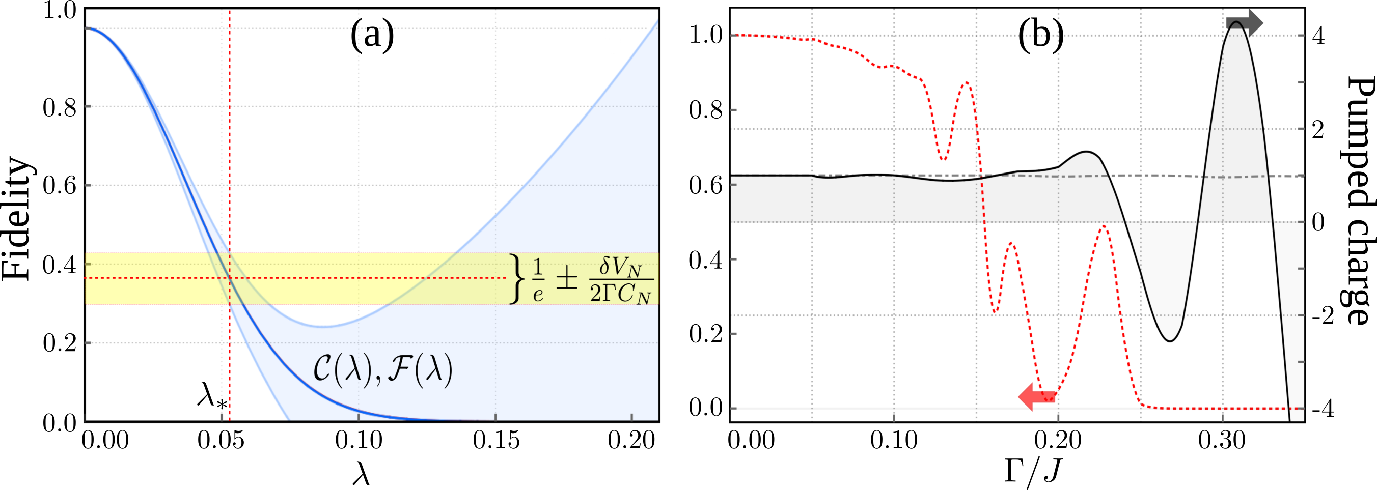
Figure 2: Adiabaticity, orthogonality catastrophe and transport in a Thouless pump described by the Hamiltonian (12) with $N=1000$ particles. (a) Illustration of the inequality (Timescale for adiabaticity breakdown in driven many-body systems and orthogonality catastrophe). Solid blue – the orthogonality overlap $\mathcal{C}(\lambda)$. The shaded region is the one, which has to contain the $\mathcal{F}(\lambda)$ curve due to the inequality (Timescale for adiabaticity breakdown in driven many-body systems and orthogonality catastrophe). This bound is tight enough to guarantee the adiabaticity breakdown for the chosen set of parameters, $J=0.4E_{R},$ $U=0.4E_{R}$, $\Delta=\lambda E_{R}$ with $\lambda=\Gamma t$ and $\Gamma=0.7E_{R}$. For $E_{R}=6.4$ ms^-1 these parameters coincide with those of the effective Hamiltonian describing the optical lattice in the experiment Ref. Nakajima et al. (2016) at the $\Delta=0$ point of the pumping cycle. Remarkably, true adiabatic fidelity $\mathcal{F}(\lambda)$ calculated numerically follows $\mathcal{C}(\lambda)$ even closer than what can be expected from the bound (Timescale for adiabaticity breakdown in driven many-body systems and orthogonality catastrophe), so that the two curves look indistinguishable in the figure. The latter fact indicates that the sides $b$ and $c$ of the triangle depicted in Fig. 1 are in fact nearly orthogonal in the present case. (b) The charge transferred during the cycle (dash-dotted gray) as compared to the total transferred charge collected until the current vanishes (solid black) for different values of the driving rate, $\Gamma$. The cycle is given by $\Delta=(J/2)\sin\lambda$, $U=(J/2)\cos\lambda$ with $\lambda=\Gamma t$. The pump performs a single cycle and then stops. Initially the system is in equilibrium. The adiabatic fidelity $\mathcal{F}$ at the end of the cycle is shown by the dashed red line. One can see that the charge transferred during the cycle is quantized even when the many-body adiabaticity has gone completely ($\mathcal{F}\simeq 0$), while the quantization of the total transferred charge disappears as soon as the many-body adiabaticity is broken.

The Thouless pump protocol in a Rice-Mele system was recently implemented in a parabolically confined ultracold atomic system Nakajima et al. (2016) (see also Lohse et al. (2015) for pumping in a Bose-Mott insulator). The particle transport was measured by the direct observation of the centre-of-mass displacement of the atomic cloud using in situ absorption imaging. The authors of Ref. Nakajima et al. (2016) emphasise the importance of adiabaticity for the observation of the Thouless quantisation. In order to ensure slow enough driving, they use a heuristic condition $\Gamma<\Gamma_{\rm LZ}$. Here $\Gamma_{\rm LZ}$ is obtained in the Landau-Zener spirit from the condition $2\pi(D_{\rm min}/2)^{2}/(\dot{D}_{\rm max})=1$, where $D_{\rm min}$ is the smallest value of the time-dependent band gap, $D(t)$, and $\dot{D}_{\rm max}$ is the maximal derivative of $D(t)$ during the cycle. We note that this condition is insensitive to the system size, in particular it does not predict any problems with adiabaticity in the thermodynamic limit. In contrast, our exact result (6), together with the scaling laws $C_{N}\sim N$ and $\delta V_{N}\sim\sqrt{N}$ (see material to this article ) imply that for any given $\Gamma<\Gamma_{\rm LZ}$ adiabaticity fails to survive even a single cycle of pumping when the number of particles is too large . To illustrate the effect of the system size on adiabaticity we numerically simulate the evolution of the fidelity $\mathcal{F}$ in the Rice-Mele model (12)for various system sizes, with parameters $J$, $U$, $\Delta$ taken from the experiment Nakajima et al. (2016). While for $N=10$, which is close to the experimental value, the bound (Timescale for adiabaticity breakdown in driven many-body systems and orthogonality catastrophe) is too weak to relate the fidelity to the orthogonality catastrophe material to this article , for $N=1000$ the bound is strong enough to ensure an $e$-fold decay of the fidelity over a mean-free path, which turns out to be only a small fraction of the complete cycle, see Fig. 2 (a).

It is instructive to investigate what happens to the Thouless pumping in the regime where the particle number is large enough to ensure the collapse of adiabaticity within one cycle, but the driving is slow compared to the bandgap. First, we consider this question qualitatively assuming, for simplicity, a two-terminal geometry where the ends of the Rice-Mele lattice are attached to two infinite particle reservoirs. In such a geometry the charge is pumped between the two reservoirs. We recall that the adiabatic mean free path $\lambda_{*}\sim 1/\sqrt{N}$ is the typical distance the Thouless pump travels in the parameter space before an elementary excitation is created in the bulk. For $\lambda_{*}$ much shorter than the length of the loop that the system describes in the parameter space, a large number of elementary excitations is born in one cycle. These excitations form a dilute gas of mobile quasi-particles, which travel in both directions, left and right. If the pump is initiated in the equilibrium state and performs one cycle, then during the period $T$ of the cycle the number of such excitations reaching the left/right end of the system will be $\delta N=\rho vT,$ where $\rho\sim 1/(\lambda_{*}N)$ is the number of elementary excitations created during the cycle per lattice site and $v$ is the typical group velocity. Clearly, $\delta N\ll 1$ in the large $N$ limit, therefore the charge pumped in one cycle will be close to the quantized value despite the violation of adiabaticity conditions. The quantization also survives in the steady regime of operation of the pump, when it performs one cycle after another. This has been demonstrated in Ref. Privitera et al. (2018) by analyzing the Floquet eigenstates of the pump.

However, the quantization breaks down simultaneously with adiabaticity in a yet different setting, when the pump performs a single cycle and stops, and one counts all the transferred charge, until the current vanishes (which happens long after the cycle ends). In this case all $\sim\sqrt{N}$ quasiparticles will eventually reach the reservoirs thus destroying the quantization. This conclusion is supported by a microscopic calculation (given in the Supplement) as illustrated in Fig. 2 (b).

To conclude, we have established a simple quantitative relationship between the orthogonality catastrophe and the adiabaticity breakdown in a driven many-body system. We have illustrated the utility of this finding by determining conditions for quantization of transport in a Thouless pump.

Supplement

Appendix A 1.  Quantum speed limit and relation between orthogonality catastrophe and adiabaticity

In contrast to the main text, in the present section we use time, not $\lambda$, to parameterize the instantaneous ground state of the system, $\Phi_{t}$, and the evolving state of the system, $\Psi_{t}$. The former is a solution of the Schrodinger’s stationary equation

$$\begin{array}[]{c}\displaystyle\hat{H}_{\lambda(t)}\,\Phi_{t}=E_{\lambda(t)}\,\Phi_{t},\end{array}$$ (S1)

while the latter satisfies the Schrodinger’s equation

$$\begin{array}[]{c}\displaystyle i\,\frac{\partial}{\partial t}\Psi_{t}=\hat{H}_{\lambda(t)}\,\Psi_{t}\end{array}$$ (S2)

with the initial condition $\Psi_{0}=\Phi_{0}$. Here $\lambda(t)$ can be an arbitrary smooth function of time. We will also slightly abuse the notations and write ${\cal R}(t)\equiv{\cal R}\left(\lambda(t)\right)$.

A.1 1.1.  Relation between orthogonality catastrophe and adiabaticity

Here we prove the inequality (8) of the main text which relates the orthogonality overlap $\cal C(\lambda)$ with the adiabatic fidelity $\cal F(\lambda)$. We rewrite it as follows:

$$|{\cal F}\left(\lambda(t)\right)-{\cal C}\left(\lambda(t)\right)|\leq{\cal R}(t)\equiv\int_{0}^{t}\sqrt{\langle\Psi_{0}|\hat{H}_{\lambda(t^{\prime})}^{2}|\Psi_{0}\rangle-\langle\Psi_{0}|\hat{H}_{\lambda(t^{\prime})}|\Psi_{0}\rangle^{2}}\,dt^{\prime}.$$ (S3)

Here the integration is performed over the path in the parameter space parameterised by time, and $t$ corresponds to the end point $\lambda$ of this path.

In order to prove the bound (S3) we employ the quantum speed limit (QSL) in the following form:

$$\begin{array}[]{c}\displaystyle D(\Psi_{0},\Psi_{t})~{}\leq~{}\frac{2}{\pi}\,{\cal R}(t),\end{array}$$ (S4)

where $D$ defined by Eq. (9) of the main text is a distance on the Hilbert space known as Bures angle, quantum angle or Fubini-Study metric. The QSL (S4) is a direct consequence of a more general result by Pfeifer Pfeifer (1993); Pfeifer and Fröhlich (1995). A detailed derivation of eq. (S4) can be found in the next subsection.

Combining the QSL (S4) with the triangle inequality

$$\begin{array}[]{c}\displaystyle|D(\Phi_{t},\Psi_{0})-D(\Phi_{t},\Psi_{t})|~{}\leq~{}D(\Psi_{0},\Psi_{t})\end{array}$$ (S5)

and taking into account that $\Psi_{0}=\Phi_{0}$, one gets

$$\begin{array}[]{c}\displaystyle|D(\Phi_{t},\Phi_{0})-D(\Phi_{t},\Psi_{t})|~{}\leq~{}\frac{2}{\pi}{\cal R}(t).\end{array}$$ (S6)

Finally, one obtains the inequality (S3) from the inequality (S6) by observing that

$$\begin{array}[]{c}\displaystyle|x^{2}-y^{2}|~{}\leq~{}|\arccos x-\arccos y|~{}~{}~{}{\mathrm{for~{}all}}~{}~{}~{}|x|\leq 1,~{}~{}|y|\leq 1.\end{array}$$ (S7)

One may wonder what is the reason for using the Bures angle distance instead of e.g. a more conventional trace distance, $D_{\rm tr}(\Psi,\Phi)\equiv\sqrt{1-\left|\langle\Phi|\Psi\rangle\right|^{2}}$ . It is easy to see that the trace distance is bounded by the Bures angle, $D_{\rm tr}(\Psi,\Phi)<(\pi/2)D(\Psi,\Phi)$, and thus eq. (S4) entails the following (weaker) version of the QSL,

$$\begin{array}[]{c}\displaystyle D_{tr}(\Psi_{0},\Psi_{t})~{}\leq~{}{\cal R}(t).\end{array}$$ (S8)

However, if we try to move forward with this QSL instead of eq. (S4), we get an extra factor 2 in the r.h.s. of the bound (S3). Let us show this. Using (S8) and triangle inequality for the trace distance, one obtains an analog of (S6):

$$\begin{array}[]{c}\displaystyle|D_{tr}(\Phi_{t},\Phi_{0})-D_{tr}(\Phi_{t},\Psi_{t})|~{}\leq~{}{\cal R}(t).\end{array}$$ (S9)

Now one has to relate the l.h.s. of this inequality with the l.h.s. of inequality (S3). This amounts to relating $|\sqrt{1-x^{2}}-\sqrt{1-y^{2}}|$ with $|x^{2}-y^{2}|$, and at this point extra 2 emerges. This is because one can only guarantee that

$$\begin{array}[]{c}\displaystyle|x^{2}-y^{2}|\leq 2|\sqrt{1-x^{2}}-\sqrt{1-y^{2}}|,\end{array}$$ (S10)

compare to eq. (S7).

A.2 1.2.  Quantum speed limit

Here we derive the QSL limit (S4) from a result by Pfeifer Pfeifer (1993); Pfeifer and Fröhlich (1995) which reads

$$\sin_{*}\left(\arcsin\left|\langle F|\Psi_{0}\rangle\right|-{\cal R}(t)\right)~{}\leq~{}|\langle F|\Psi_{t}\rangle|~{}\leq~{}\sin_{*}\left(\arcsin\left|\langle F|\Psi_{0}\rangle\right|+{\cal R}(t)\right).$$ (S11)

Here $F$ is an arbitrary auxiliary state and

$$\begin{array}[]{c}\displaystyle\sin_{*}x\equiv\left\{\begin{array}[]{ll}0,&x<0,\\ \sin x,&0\leq x\leq\pi/2,\\ 1,&x>\pi/2.\end{array}\right.\end{array}$$ (S12)

Noting that $\arcsin x+\arccos x=\pi/2$ and $\sin_{*}(\pi/2-x)=\cos_{*}x$ with

$$\begin{array}[]{c}\displaystyle\cos_{*}x\equiv\left\{\begin{array}[]{ll}1,&x<0,\\ \cos x,&0\leq x\leq\pi/2,\\ 0,&x>\pi/2,\end{array}\right.\end{array}$$ (S13)

one can rewrite (S11) as

$$\cos_{*}\left(\arccos\left|\langle F|\Psi_{0}\rangle\right|+{\cal R}(t)\right)~{}\leq~{}|\langle F|\Psi_{t}\rangle|~{}\leq~{}\cos_{*}\left(\arccos\left|\langle F|\Psi_{0}\rangle\right|-{\cal R}(t)\right).$$ (S14)

Taking into account that

$$\begin{array}[]{c}\displaystyle\arccos(\cos_{*}x)=\left\{\begin{array}[]{ll}0,&x<0,\\ x,&0\leq x\leq\pi/2,\\ \pi/2,&x>\pi/2,\end{array}\right.\end{array}$$ (S15)

one rewrites eq. (S14) in terms of the Bures angle:

$$\max\{D(F,\Psi_{0})-\frac{2}{\pi}\,{\cal R}(t),0\}~{}\leq~{}D(F,\Psi_{t})~{}\leq~{}\min\{D(F,\Psi_{0})+\frac{2}{\pi}\,{\cal R}(t),1\}.$$ (S16)

Employing obvious relations $\min\{x,y\}\leq x$ and $\max\{x,y\}\geq x$ one reduces (S16) to a more compact, though slightly more rough inequality,

$$\begin{array}[]{c}\displaystyle\left|D(F,\Psi_{t})-D(F,\Psi_{0})\right|~{}\leq~{}\frac{2}{\pi}\,{\cal R}(t).\end{array}$$ (S17)

Choosing $F=\Psi_{0}$ one obtains the QSL (S4).

It should be noted that another choice, $F=\Phi_{t}$, directly reduces the inequality (S17) (along with the condition $\Psi_{0}=\Phi_{0}$) to the inequality (S6). Such a direct route which apparently dispenses with the triangle inequality is possible because Pfeifer’s rather sophisticated result has, in fact, a more broad scope than elementary versions of the quantum speed limit and contains the triangle inequality built in.

Appendix B 2.  Rice-Mele model

B.1 2.1.  Eigenstates and eigenenergies

The transformation

$$a_{j}=\frac{1}{\sqrt{N}}\sum_{k}e^{ikj}a_{k},~{}~{}b_{j}=\frac{1}{\sqrt{N}}\sum_{k}e^{ikj}b_{k},~{}~{}k=\frac{2\pi}{N}l,~{}~{}l=-\frac{N}{2}+1,-\frac{N}{2}+2,...,\frac{N}{2},$$ (S18)

where $N$ is assumed to be even, allows one to represent the Rice-Mele Hamiltonian, eq. (12) in the main text, as a sum of $N$ commuting terms,

$$\begin{array}[]{c}\displaystyle\hat{H}_{\rm RM}=\sum_{k}(a^{\dagger}_{k}~{}b^{\dagger}_{k})\left(\begin{array}[]{c c}\Delta&-(J+U)-(J-U)e^{ik}\\ -(J+U)-(J-U)e^{-ik}&-\Delta\end{array}\right)\left(\begin{array}[]{c }a_{k}\\ b_{k}\end{array}\right).\end{array}$$ (S19)

Observe that $n_{k}\equiv a^{\dagger}_{k}a_{k}+b^{\dagger}_{k}b_{k}$ is conserved for each $k$. We assume half-filling, i.e. that the total number of particles equals $N$. In this case the ground state of the Hamiltonian for any values of $(J,U,\Delta)$ is an eigenstate of $n_{k}$ with the eigenvalue equal to 1, and this is maintained throughout the evolution. Restricting the Hamiltonian (S19) to the corresponding subspace one obtains an effective Hamiltonian of $N$ noninteracting spins,

$$\begin{array}[]{c}\displaystyle\hat{H}_{\rm RM}=\sum_{k}{\boldsymbol{p}_{k}}\cdot\boldsymbol{\sigma}_{k},~{}~{}~{}~{}~{}~{}~{}~{}~{}{\boldsymbol{p}_{k}}=\left(\begin{array}[]{c }-(J+U)-(J-U)\cos k\\ (J-U)\sin k\\ \Delta\end{array}\right),\end{array}$$ (S20)

where $\boldsymbol{\sigma}$ is a vector consisting of three Pauli matrices. Each two-level Hamiltonian $\hat{H}_{k}\equiv{\boldsymbol{p}_{k}}\cdot\boldsymbol{\sigma}_{k}$ has two eigenstates $|\chi_{k}^{\pm}\rangle$ and eigenenergies $\varepsilon_{k}^{\pm}$,

$$\begin{array}[]{c}\displaystyle\rho_{k}^{\pm}\equiv|\chi_{k}^{\pm}\rangle\langle\chi_{k}^{\pm}|=\frac{1}{2}(1\pm\frac{1}{|\boldsymbol{p}_{k}|}\,{\boldsymbol{p}_{k}}\cdot\boldsymbol{\sigma}_{k}),~{}~{}~{}~{}~{}~{}~{}~{}~{}~{}\varepsilon_{k}^{\pm}=\pm\sqrt{2(J^{2}+U^{2})+\Delta^{2}+2(J^{2}-U^{2})\cos k}.\end{array}$$ (S21)

The ground state of the whole system is the product of $N$ single-spin eigenstates, $|\Phi\rangle=\prod\limits_{k}\otimes|\chi_{k}^{-}\rangle$ while the ground state energy is the sum of corresponding eigenenergies, $E=\sum\limits_{k}\varepsilon_{k}^{-}$.

B.2 2.2.  Orthogonality catastrophe

Here we consider the orthogonality catastrophe induced by changing the parameters of the Hamiltonian $(J,U,\Delta)$ along some trajectory parameterized by $\lambda$. This is to say that $(J,U,\Delta)$ and thus vectors $\boldsymbol{p}_{k}$ are functions of $\lambda$. In contrast to the main text, we do not employ the convention that $\lambda=0$ at $t=0$.

The orthogonality overlap for a single spin reads

$$\begin{array}[]{c}\displaystyle\mathfrak{c}_{k}(\lambda^{\prime},\lambda)\equiv|\langle\chi_{k}^{-}(\lambda^{\prime})|\chi_{k}^{-}(\lambda)\rangle|^{2}={\rm tr}(\rho_{k}^{-}(\lambda)\rho_{k}^{-}(\lambda^{\prime}))=\frac{1}{2}(1+\frac{\boldsymbol{p}_{k}(\lambda)\cdot\boldsymbol{p}_{k}(\lambda^{\prime})}{|\boldsymbol{p}_{k}(\lambda)|\,|\boldsymbol{p}_{k}(\lambda^{\prime})|}).\end{array}$$ (S22)

The orthogonality overlap for the whole many-body system is given by

$$\begin{array}[]{c}\displaystyle\mathcal{C}(\lambda^{\prime},\lambda;N)\equiv|\langle\Phi_{\lambda^{\prime}}|\Phi_{\lambda}\rangle|^{2}=\exp\left(-\sum_{k}\log\frac{1}{\mathfrak{c}_{k}}\right).\end{array}$$ (S23)

Further,

$$\begin{array}[]{c}\displaystyle C_{N}=\sum_{k}\,c_{k}~{}~{}~{}{\rm with}~{}~{}~{}c_{k}\equiv-\frac{1}{2}\left.\left(\frac{\partial^{2}}{\partial\lambda^{2}}\log\mathfrak{c}_{k}(\lambda^{\prime},\lambda)\right)\right|_{\lambda^{\prime}=\lambda}=\frac{1}{4}\left(\frac{\partial_{\lambda}\boldsymbol{p}_{k}\cdot\partial_{\lambda}\boldsymbol{p}_{k}}{|\boldsymbol{p}_{k}|^{2}}-\frac{(\boldsymbol{p}_{k}\cdot\partial_{\lambda}\boldsymbol{p}_{k})^{2}}{|\boldsymbol{p}_{k}|^{4}}\right).\end{array}$$ (S24)

This equation along with eq. (S20) enables one to calculate $C_{N}$ for any point of any trajectory in the parameter space of the Rice-Mele model. For example, for $J,U={\rm const}$, $\Delta=\lambda E_{R}$ one obtains

$$\begin{array}[]{c}\displaystyle c_{k}=\frac{1}{8}\frac{1}{J^{2}+U^{2}+(J^{2}-U^{2})\cos k}\end{array}$$ (S25)

and

$$C_{N}=\frac{NE_{R}^{2}}{16JU}.$$ (S26)

B.3 2.3.  Quantum uncertainty of the driving potential

To deal with general trajectories we define the driving term as

$$\begin{array}[]{c}\displaystyle\hat{V}\equiv\partial_{\lambda}\hat{H}_{\lambda},\end{array}$$ (S27)

which is consistent with the definition adopted in the main text. For the Rice-Mele model

$$\begin{array}[]{c}\displaystyle\hat{V}=\sum_{k}\partial_{\lambda}\boldsymbol{p}_{k}\cdot\boldsymbol{\sigma}_{k}.\end{array}$$ (S28)

Since the ground state is of the product form, the quantum uncertainty of $\hat{V}$ is expressed through individual uncertainties of states of single spins:

$$\begin{array}[]{c}\displaystyle\delta V^{2}=\sum_{k}\left({\rm tr}\left(\rho_{k}^{-}\,(\partial_{\lambda}\boldsymbol{p}_{k}\cdot\boldsymbol{\sigma}_{k})^{2}\right)-\left({\rm tr}\left(\rho_{k}^{-}\,\partial_{\lambda}\boldsymbol{p}_{k}\cdot\boldsymbol{\sigma}_{k}\right)\right)^{2}\right)=\sum_{k}\left(|\partial_{\lambda}\boldsymbol{p}_{k}|^{2}-\frac{(\boldsymbol{p}_{k}\cdot\partial_{\lambda}\boldsymbol{p}_{k})^{2}}{|\boldsymbol{p}_{k}|^{2}}\right).\end{array}$$ (S29)

This equation along with eq. (S20) allows one to calculate $\delta V_{N}$ for any point of any trajectory in the parameter space of the Rice-Mele model. For example, for $J,U={\rm const}$, $\Delta=\lambda E_{R}$ one gets

$$\delta V_{N}^{\rm RM}=\sqrt{N}E_{R}.$$ (S30)

With the knowledge of $C_{N}$ and $\delta V_{N}$ one can make practical use of the inequality (8) of the main text, or, alternatively, inequality (S3). For a fixed $\Gamma$ the r.h.s. of this inequality inevitably diminishes with growing $N$, leading to $\mathcal{F}(\lambda)\simeq\mathcal{C}(\lambda)$, as illustrated in Fig. 2 (a) of the main text. The opposite situation when the r.h.s. of (S3) is large and thus the inequality (S3) is inconclusive is illustrated in Fig. 3.

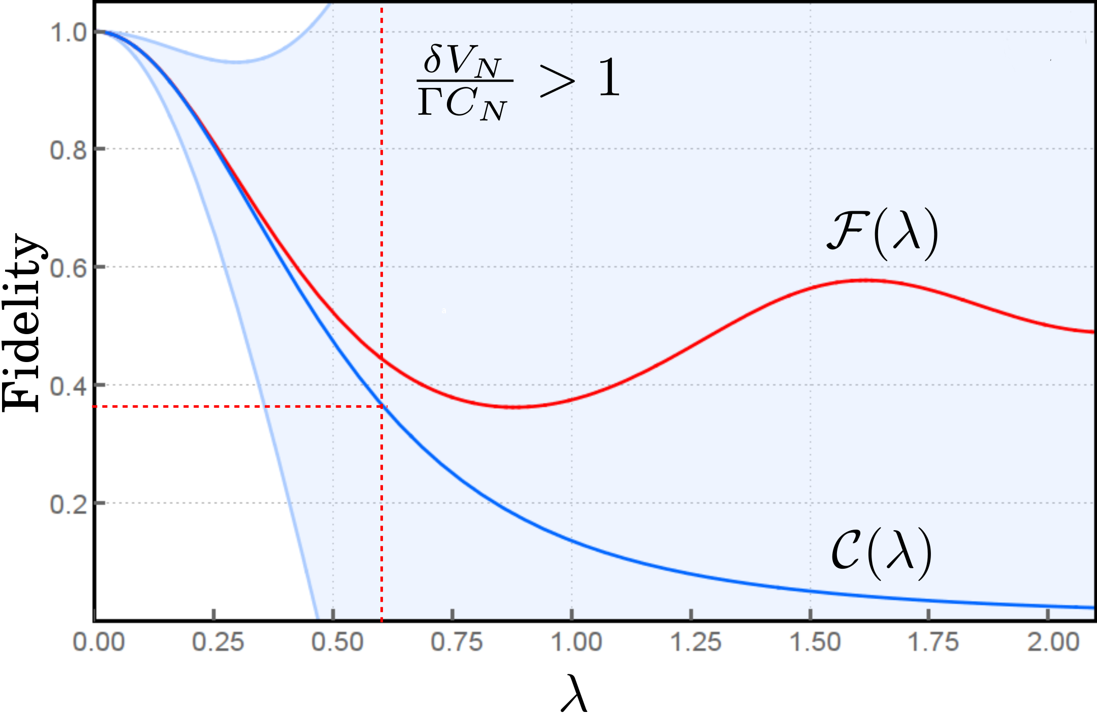
Figure 3: Evolution of the ground state fidelity in the parameter space of the Hamiltonian (S19) for $N=10$ particles. The fidelity $\mathcal{F}$ is shown as a solid red curve, while the overlap function $\mathcal{C}$ is shown as a solid blue curve. The shaded region is the one, which has to contain the $\mathcal{F}(\lambda)$ curve due to the inequality (S3). For $N=10$ the inequality (S3) does not impose a meaningful upper bound on the fidelity, and therefore has nothing to say about the relationship between the fidelity and the orthogonality catastrophe. The parameters used read $J=0.4E_{R},$ $U=0.4E_{R}$ and $\Delta=\lambda E_{R}$ with $\lambda=\Gamma t$ and $\Gamma=0.7E_{R}.$ For the recoil energy $E_{R}=6.4$ ms^-1 these coincide with the parameters of the effective Hamiltonian describing the optical lattice in the experiment Ref. Nakajima et al. (2016) at the $\Delta=0$ point of the pumping cycle.

B.4 2.4.  Current and transferred charge

The current flowing between the $l$’th and $(l+1)$’th elementary cell reads

$$\begin{array}[]{c}\displaystyle\hat{j}_{l}=i(J-U)\sum_{l=1}^{N}(b_{l+1}^{\dagger}a_{l}-a_{l}^{\dagger}b_{l+1}).\end{array}$$ (S31)

Due to translation invariance of the Hamiltonian and the initial state the current is the same for all cells. It is convenient to define an average current,

$$\begin{array}[]{c}\displaystyle\hat{j}\equiv\frac{1}{N}\sum_{l=0}^{N}\hat{j}_{l},\end{array}$$ (S32)

and then express it in terms of $a_{k}$, $b_{k}$:

$$\begin{array}[]{c}\displaystyle\hat{j}=\frac{i}{N}\sum_{k}(a^{\dagger}_{k}~{}b^{\dagger}_{k})\left(\begin{array}[]{c c}0&-(J-U)e^{ik}\\ (J-U)e^{-ik}&0\end{array}\right)\left(\begin{array}[]{c }a_{k}\\ b_{k}\end{array}\right).\end{array}$$ (S33)

In terms of spin variables the current can be written as

$$\begin{array}[]{c}\displaystyle\hat{j}=\frac{1}{N}\sum_{k}\hat{j}_{k}~{}~{}~{}{\rm with}~{}~{}~{}\hat{j}_{k}={\boldsymbol{j}_{k}}\cdot\boldsymbol{\sigma}_{k},~{}~{}~{}~{}~{}~{}{\boldsymbol{j}_{k}}=\left(\begin{array}[]{c }(J-U)\sin k\\ (J-U)\cos k\\ 0\end{array}\right),\end{array}$$ (S34)

The pumped charge is the integral of the quantum average of this current over the elapsed time:

$$\begin{array}[]{c}\displaystyle Q(t)=\int_{0}^{t}dt^{\prime}\,\langle\Psi_{t^{\prime}}|\hat{j}|\Psi_{t^{\prime}}\rangle.\end{array}$$ (S35)

Thanks to eq. (S20) and factorized initial condition $\Psi_{0}=\Phi_{0}=\prod\limits_{k}\chi^{-}_{k}$, eq. (S35) can be written as

$$\begin{array}[]{c}\displaystyle Q(t)=\int_{0}^{t}dt^{\prime}\sum_{k}\langle\chi_{k}(t^{\prime})|\hat{j}_{k}|\chi_{k}(t^{\prime})\rangle,\end{array}$$ (S36)

where $\chi_{k}(t)$ is found from the Schrodinger equation

$$\begin{array}[]{c}\displaystyle i\,\partial_{t}\,\chi_{k}(t)=({\boldsymbol{p}_{k}}(t)\cdot\boldsymbol{\sigma}_{k})\,\chi_{k}(t).\end{array}$$ (S37)

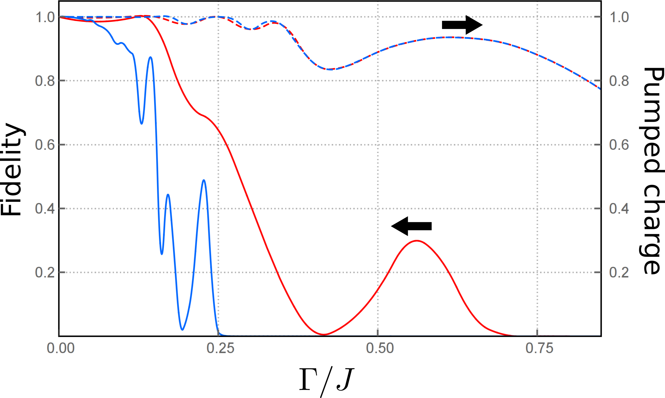
Figure 4: Fidelity (solid curves) and pumped charge (dashed curves) after a single cycle in the Rice-Mele realisation of the Thouless pump, eq. (S19). The trajectory of the cycle is given by $\Delta=(J/2)\sin\lambda$, $U=(J/2)\cos\lambda$ with $\lambda=\Gamma t$. The system is initiated in equilibrium. Red and blue curves correspond to $N=100$ and $N=1000$ fermions in a lattice, respectively. One can see that the charge transferred in a single cycle hardly depends on the number of particles for $N\gtrsim 100$ while the fidelity decays more rapidly for larger $N$.

In the context of Thouless pumping we enquire how much charge is transferred per cycle immediately after the cycle is over, and long after the cycle is over. To answer the former question we calculate $Q(t)$ by solving the Schrodinger equations (S37) numerically. The result is illustrated in Fig. 4. The latter question is addressed by counting the number of right- and left- moving excitations produced during the cycle. To this end we define the average population of the excited state with the quasimomentum $k$,

$$\begin{array}[]{c}\displaystyle w_{k}=\langle\chi_{k}(T)|\frac{1}{2}(1+{\boldsymbol{p}_{k}}(T)\cdot\boldsymbol{\sigma}_{k})|\chi_{k}(T)\rangle.\end{array}$$ (S38)

Remind that $\chi_{k}(T)$ should be found numerically from the Schrodinger equation (S37). Taking into account that ${\boldsymbol{p}_{k}}(T)={\boldsymbol{p}_{k}}(0)$ this can be rewritten with the use of eq. (S21) as

$$\begin{array}[]{c}\displaystyle w_{k}=|\langle\chi_{k}^{+}|\chi_{k}(T)\rangle|^{2}.\end{array}$$ (S39)

The sign of the group velocity of the excitations, $\partial(\varepsilon_{k}^{+}-\varepsilon_{k}^{-})/\partial k$, coincides with the sign of $k$ for $-\pi<k<\pi$, as is clear from eq. (S21). Therefore the charge transferred from left to right per cycle in the steady state, $\Delta Q$, reads

$$\begin{array}[]{c}\displaystyle\Delta Q=\sum_{0<k<\pi}w_{k}-\sum_{-\pi<k<0}w_{k}.\end{array}$$ (S40)

References

- Born (1926) Max Born, “Das adiabatenprinzip in der quantenmeehanik,” Zeitschrift für Physik 40, 167 (1926).
- Born and Fock (1928) Max Born and Vladimir Fock, “Beweis des adiabatensatzes,” Zeitschrift für Physik 51, 165–180 (1928).
- Avron and Elgart (1999) Joseph E Avron and Alexander Elgart, “Adiabatic theorem without a gap condition,” Communications in mathematical physics 203, 445–463 (1999).
- Alexander L. Fetter (2003) John Dirk Walecka Alexander L. Fetter, Quantum Theory of Many-Particle Systems, Dover Books on Physics (Dover Publications, 2003).
- Nenciu and Rasche (1989) G Nenciu and G Rasche, “Adiabatic theorem and gell-mann-low formula,” Helvetica Physica Acta 62, 372–388 (1989).
- Car and Parrinello (1985) Richard Car and Mark Parrinello, “Unified approach for molecular dynamics and density-functional theory,” Physical Review Letters 55, 2471 (1985).
- Budich and Trauzettel (2013) Jan Carl Budich and Björn Trauzettel, “From the adiabatic theorem of quantum mechanics to topological states of matter,” physica status solidi (RRL)-Rapid Research Letters 7, 109–129 (2013).
- Montanaro (2016) Ashley Montanaro, “Quantum algorithms: an overview,” npj Quantum Information 2, 15023 (2016).
- Nakamura (2012) Hiroki Nakamura, Nonadiabatic transition : concepts, basic theories and applications, 2nd ed. (World Scientific, 2012).
- Messiah (2014) Albert Messiah, Quantum Mechanics, Dover Books on Physics (Dover Publications, 2014).
- Landau (1932) Lev D Landau, “Zur theorie der energieubertragung. ii,” Physics of the Soviet Union 2, 28 (1932).
- Zener (1932) Clarence Zener, “Non-adiabatic crossing of energy levels,” in Proceedings of the Royal Society of London A: Mathematical, Physical and Engineering Sciences, Vol. 137 (The Royal Society, 1932) pp. 696–702.
- Marzlin and Sanders (2004) Karl-Peter Marzlin and Barry C Sanders, “Inconsistency in the application of the adiabatic theorem,” Physical Review Letters 93, 160408 (2004).
- Tong et al. (2005) DM Tong, K Singh, LC Kwek, and CH Oh, “Quantitative conditions do not guarantee the validity of the adiabatic approximation,” Physical Review Letters 95, 110407 (2005).
- Jansen et al. (2007) Sabine Jansen, Mary-Beth Ruskai, and Ruedi Seiler, “Bounds for the adiabatic approximation with applications to quantum computation,” Journal of Mathematical Physics 48, 102111 (2007).
- Lidar et al. (2009) Daniel A Lidar, Ali T Rezakhani, and Alioscia Hamma, “Adiabatic approximation with exponential accuracy for many-body systems and quantum computation,” Journal of Mathematical Physics 50, 102106 (2009).
- Bachmann et al. (2017) Sven Bachmann, Wojciech De Roeck, and Martin Fraas, “The adiabatic theorem for many-body quantum systems,” Phys. Rev. Lett. 119, 060201 (2017).
- Polkovnikov and Gritsev (2008) A. Polkovnikov and V. Gritsev, “Breakdown of the adiabatic limit in low-dimensional gapless systems,” Nature Phys. 4, 477–481 (2008).
- Altland and Gurarie (2008) A. Altland and V. Gurarie, “Many body generalization of the Landau-Zener problem,” Phys. Rev. Lett. 100, 063602 (2008).
- Altland et al. (2009) A. Altland, V. Gurarie, T. Kriecherbauer, and A. Polkovnikov, “Nonadiabaticity and large fluctuations in a many-particle Landau-Zener problem,” Phys. Rev. A 79, 042703 (2009).
- Shytov (2004) AV Shytov, “Landau-zener transitions in a multilevel system: An exact result,” Physical Review A 70, 052708 (2004).
- Lychkovskiy (2015) O. Lychkovskiy, “Perpetual motion and driven dynamics of a mobile impurity in a quantum fluid,” Phys. Rev. A 91, 040101 (2015).
- Schecter et al. (2015) Michael Schecter, Dimitri M. Gangardt, and Alex Kamenev, “Comment on “Kinetic theory for a mobile impurity in a degenerate tonks-girardeau gas”,” Phys. Rev. E 92, 016101 (2015).
- Gamayun et al. (2015) O. Gamayun, O. Lychkovskiy, and V. Cheianov, “Reply to “Comment on ‘Kinetic theory for a mobile impurity in a degenerate Tonks-Girardeau gas’ ”,” Phys. Rev. E 92, 016102 (2015).
- Mahan (2000) Gerald D. Mahan, Many-particle Physics (Kluwer Academic/Plenum Publishers, 2000).
- Gull et al. (2011) Emanuel Gull, Andrew J Millis, Alexander I Lichtenstein, Alexey N Rubtsov, Matthias Troyer, and Philipp Werner, “Continuous-time monte carlo methods for quantum impurity models,” Reviews of Modern Physics 83, 349 (2011).
- Gebert et al. (2014) Martin Gebert, Heinrich Küttler, and Peter Müller, “Anderson’s orthogonality catastrophe,” Communications in Mathematical Physics 329, 979–998 (2014).
- (28) Martin Gebert, Heinrich Küttler, Peter Müller, and Peter Otte, “The exponent in the orthogonality catastrophe for fermi gases,” J. Spectr. Theory 6, 643-683 (2016) .
- Rivier and Simanek (1971) N Rivier and E Simanek, “Exact calculation of the orthogonality catastrophe in metals,” Physical Review Letters 26, 435 (1971).
- Hamann (1971) DR Hamann, “Orthogonality catastrophe in metals,” Physical Review Letters 26, 1030 (1971).
- Kaga and Yosida (1978) Hiroyuki Kaga and Kei Yosida, “Orthogonality catastrophe due to local electron correlation,” Progress of Theoretical Physics 59, 34–39 (1978).
- Janis (1997) V Janis, “Complete wiener-hopf solution of the x-ray edge problem,” Int. J. Mod. Phys. B 11, 3433 (1997).
- Note (1) Up to Poincare revivals. Their time scale increases so rapidly with increasing system size that they can be safely ignored in in both practical and asymptotic sense.
- (34) See Supplementary material to this article, .
- Bengtsson and Zyczkowski (2007) Ingemar Bengtsson and Karol Zyczkowski, Geometry of quantum states: an introduction to quantum entanglement (Cambridge University Press, 2007).
- Pfeifer (1993) Peter Pfeifer, “How fast can a quantum state change with time?” Phys. Rev. Lett. 70, 3365 (1993).
- Pfeifer and Fröhlich (1995) Peter Pfeifer and Jürg Fröhlich, “Generalized time-energy uncertainty relations and bounds on lifetimes of resonances,” Reviews of Modern Physics 67, 759 (1995).
- Anderson (1967) Philip W Anderson, “Infrared catastrophe in fermi gases with local scattering potentials,” Physical Review Letters 18, 1049 (1967).
- Gefen et al. (2002) Yuval Gefen, Richard Berkovits, Igor V Lerner, and Boris L Altshuler, “Anderson orthogonality catastrophe in disordered systems,” Physical Review B 65, 081106 (2002).
- Kettemann (2016) S. Kettemann, “Exponential orthogonality catastrophe at the anderson metal-insulator transition,” Phys. Rev. Lett. 117, 146602 (2016).
- Polkovnikov and Gritsev (2011) Anatoli Polkovnikov and Vladimir Gritsev, “Universal dynamics near quantum critical points,” Understanding Quantum Phase Transitions , 59–90 (2011).
- Thouless (1983) DJ Thouless, “Quantization of particle transport,” Physical Review B 27, 6083 (1983).
- Nakajima et al. (2016) Shuta Nakajima, Takafumi Tomita, Shintaro Taie, Tomohiro Ichinose, Hideki Ozawa, Lei Wang, Matthias Troyer, and Yoshiro Takahashi, “Topological thouless pumping of ultracold fermions,” Nature Physics (2016).
- Lohse et al. (2015) Michael Lohse, Christian Schweizer, Oded Zilberberg, Monika Aidelsburger, and Immanuel Bloch, “A thouless quantum pump with ultracold bosonic atoms in an optical superlattice,” Nature Physics (2015).
- Note (3) This scaling exemplifies a remarkable fact: In a many-body system a finite energy gap is not sufficient to protect adiabaticity in the thermodynamic limit. This fact can be easily inferred from our general scaling analysis for .
- Privitera et al. (2018) Lorenzo Privitera, Angelo Russomanno, Roberta Citro, and Giuseppe E. Santoro, “Nonadiabatic breaking of topological pumping,” Phys. Rev. Lett. 120, 106601 (2018).