Low-temperature interfaces: Prewetting, layering, faceting and Ferrari–Spohn diffusions

Abstract.

In this paper, we survey and discuss various surface phenomena such as prewetting, layering and faceting for a family of two- and three-dimensional low-temperature models of statistical mechanics, notably Ising models and $2+1$-dimensional solid-on-solid (SOS) models, with a particular accent on scaling regimes which lead or, in most cases, are conjectured to lead to Ferrari–Spohn type diffusions.

1. Introduction and structure of the paper

Ferrari–Spohn (FS) diffusions were introduced in [34] as cube-root scaling limits of Brownian motion constrained to stay above circular and parabolic barriers. It turns out that FS diffusions and their Dyson counterparts are the universal scaling limits for a class of random walks [48] or, respectively, ordered random walks [50] under generalized area tilts.

Random walks under vanishing area tilts naturally appear as effective descriptions for either phase separation lines in two-dimensional models of Statistical mechanics in regimes related to critical prewetting, or for level lines of random low-temperature surfaces in three dimensions, in the regime when the number of layers grows and/or when the linear size of the system goes to infinity.

Making the above statement precise sets up the stage for a host of open problems, some of them — for instance those which arise in the context of Ising interfaces in three dimensions — seem, for the moment, notoriously difficult. On the other hand, phase separation lines in two dimensions and level lines of SOS interfaces are more tractable objects, and we expect progress in understanding FS scaling for the latter in a foreseeable future.

The paper is organized as follows: In Section 2 we try to survey the existing rigorous results and many remaining unsolved issues on wetting transition, mostly in context of Ising models on $\mathbb{Z}^{d}$. Critical prewetting, which is the somehow central notion of the scaling phenomena in question, is discussed in Section 3. Various types of 2+1-dimensional SOS-type models are discussed in Section 4, including models with hard-wall constraint (entropic repulsion), bulk and boundary fields and models coupled with high- and low-density Bernoulli fields below and above the interfaces.

Rigorous results on scaling of non-colliding random walks under area tilts are collected and briefly explained in Section 5.

Definitions and properties of Wulff shapes, the definition of FS and Dyson FS diffusions, as well as a sketch of a strategy to prove FS-scaling for self-avoiding walks under area tilts are relegated to Appendix A, Appendix B and Appendix C respectively.

2. The wetting transition

Consider a system with (at least) two thermodynamically stable phases $A$ and $B$. We assume that the bulk of the system is occupied by phase $A$ and that the latter interacts with a substrate favoring phase $B$. In such a situation, depending on how much preference the substrate displays for phase $B$, two different scenarios are possible:

$\bullet$ The bulk phase is in contact with the substrate, with only microscopic droplets of phase $B$ attached to the latter. This is called the regime of partial wetting (of the substrate by phase $B$).

$\bullet$ A mesoscopic layer of phase $B$ covers the substrate, thus separating the latter from the bulk phase. This is known as the regime of complete wetting (of the substrate by phase $B$).

The phase transition from one behavior to the other, usually triggered by a change of temperature (although it is often more convenient mathematically to use a change in the interaction between the substrate and the phases) is known as the wetting transition; the latter is a prime example of a surface phase transition.

In the remainder of this section, we discuss the phenomenon of wetting in some specific two- and three-dimensional systems. In order to keep the discussion as concrete as possible, we limit most of it to the Ising model and, in Section 4, to the corresponding effective interface models. We shall also make a few remarks on the analogous phenomena occurring in the Blume–Capel model. The general phenomenology described here has, of course, a much broader domain of validity.

2.1. The wetting transition in the Ising model

Let

$$\mathbb{H}_{+}^{d}\stackrel{{\scriptstyle\text{\tiny{\rm def}}}}{{=}}\left\{i=(i_{1},\ldots,i_{d})\in\mathbb{Z}^{d}\,:\,i_{d}\geq 0\right\}$$

and $\mathbb{H}_{-}^{d}\stackrel{{\scriptstyle\text{\tiny{\rm def}}}}{{=}}\mathbb{Z}^{d}\setminus\mathbb{H}_{+}^{d}$. Let $\beta,h\geq 0$ and set

$$J_{i,j}\stackrel{{\scriptstyle\text{\tiny{\rm def}}}}{{=}}\begin{cases}1&\text{if }\{i,j\}\subset\mathbb{H}_{+}^{d},\\ h&\text{otherwise.}\end{cases}$$ (1)

We consider the nearest-neighbor ferromagnetic Ising model in the box

$$\Delta_{n}\stackrel{{\scriptstyle\text{\tiny{\rm def}}}}{{=}}\{-n,\ldots,n\}^{d-1}\times\{0,\ldots 2n\}$$

with Hamiltonian (see Figure 1)

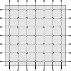
Figure 1. The box $\Delta_{3}$ with $\pm$ boundary condition (in $\mathbb{Z}^{2}$). The thick edges indicate the modified interaction between the spins in the bottom row of $\Delta_{3}$ and their neighbor in the substrate.

$$\mathcal{H}_{n;h}(\sigma)\stackrel{{\scriptstyle\text{\tiny{\rm def}}}}{{=}}-\sum_{\{i,j\}\cap\Delta_{n}\neq\varnothing}J_{i,j}\sigma_{i}\sigma_{j}.$$ (2)

In other words, the interaction between the spins located on the bottom “face” of $\Delta_{n}$ and their neighbor below them is modified; this models the interaction of the system with a substrate.

We consider two sets of configurations:

$$\Omega_{n}^{\pm}\stackrel{{\scriptstyle\text{\tiny{\rm def}}}}{{=}}\bigl{\{}\sigma\in\{\pm 1\}^{\mathbb{Z}^{d}}\,:\,\sigma_{i}=1\text{ if }i\in\mathbb{H}_{+}^{d}\setminus\Delta_{n}\text{ and }\sigma_{i}=-1\text{ if }i\in\mathbb{H}_{-}^{d}\bigr{\}}$$ (3)

and

$$\Omega_{n}^{-}\stackrel{{\scriptstyle\text{\tiny{\rm def}}}}{{=}}\bigl{\{}\sigma\in\{\pm 1\}^{\mathbb{Z}^{d}}\,:\,\sigma_{i}=-1\text{ for all }i\not\in\Delta_{n}\bigr{\}}.$$

The corresponding Gibbs measures are then defined by

$$\mu^{\pm}_{n;\beta,h}(\sigma)\stackrel{{\scriptstyle\text{\tiny{\rm def}}}}{{=}}\mathbf{1}_{\{\sigma\in\Omega_{\Delta_{n}}^{\pm}\}}\frac{e^{-\beta\mathcal{H}_{n;h}(\sigma)}}{\mathsf{Z}_{\Delta_{n};\beta,h}^{\pm}}\quad\text{ and }\quad\mu^{-}_{n;\beta,h}(\sigma)\stackrel{{\scriptstyle\text{\tiny{\rm def}}}}{{=}}\mathbf{1}_{\{\sigma\in\Omega_{\Delta_{n}}^{-}\}}\frac{e^{-\beta\mathcal{H}_{n;h}(\sigma)}}{\mathsf{Z}_{\Delta_{n};\beta,h}^{-}}.$$

We shall always assume that $\beta>\beta_{\mathrm{c}}(d)$, where $\beta_{\mathrm{c}}(d)\in(0,\infty)$ is the inverse critical temperature of the model. In this regime, typical configurations (for large $n$) are best characterized in terms of the corresponding Peierls contours, that is, the maximal connected components of the boundary of the set

$$\bigcup_{i\in\mathbb{Z}^{d}:\sigma_{i}=-1}\left\{x\in\mathbb{R}^{d}\,:\,\|x-i\|_{\scriptscriptstyle\infty}\leq 1/2\right\}.$$

Note that, under $\mu^{-}_{n;\beta,h}$, $-$ spins are favored along the inner boundary of the box $\Delta_{n}$, which always result in the $-$ phase filling the box. The situation is more interesting under $\mu^{\pm}_{n;\beta,h}$, since then the bottom side (corresponding to the substrate) favors $-$ spins, while the other sides favor $+$ spins. It is this competition that will lead to the wetting transition.

2.1.1. Entropic repulsion when $h=1$.

Let us first consider the simpler problem in which $h=1$. In this case, under the measure $\mu^{\pm}_{n;\beta,h=1}$, the boundary condition induces an interface and it is natural to investigate what effect the bottom wall has on the interface. In [37], it is proved that, at any temperature and in any dimension, the interface is repelled infinitely far away from the wall as $n\to\infty$, in the sense that the weak limits of $\mu^{-}_{n;\beta,h=1}$ and $\mu^{\pm}_{n;\beta,h=1}$ as $n\to\infty$ coincide (which means that the layer of $-$ phase along the wall extends infinitely far away from the wall). In the same paper, this was shown to imply also a weak form of delocalization of the interface at sufficiently low temperature. In dimensions $d\geq 3$ and at low enough temperatures, these delocalization results can be considerably strengthened [40], proving that “most” of the interface lies at a height of order $\log n$ above the wall. This phenomenon is known as entropic repulsion.

The issue of wetting becomes now clear: when $|h|<1$, it becomes energetically favorable for the interface to lie along the substrate, and this attraction will compete with entropic repulsion: partial wetting will occur when attraction wins, while complete wetting will occur when entropic repulsion wins. Let us now discuss these issues in more detail.

2.1.2. The two-dimensional case.

In this section, we describe some results that have been obtained concerning the wetting transition in the two-dimensional Ising model.

Observe that all configurations in $\Omega_{n}^{\pm}$ possess a unique Peierls contour $\gamma$ of infinite length. In fact, with $\mu^{\pm}_{n;\beta,h}$-probability going to $1$ as $n\to\infty$, all other contours are of diameter at most $K(\beta)\log n$ for some $K(\beta)<\infty$.

The behavior of the contour $\gamma$ depends very strongly on the value of the parameter $h$. Namely, there exists $h_{\mathrm{w}}=h_{\mathrm{w}}(\beta)\geq 0$ such that, with $\mu^{\pm}_{n;\beta,h}$-probability going to $1$ as $n\to\infty$, the following occurs (see Figure 2):

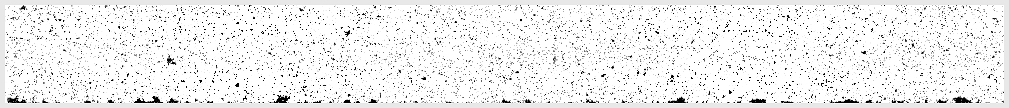
Partial wetting ($0\leq h\leq h_{\mathrm{w}}$)

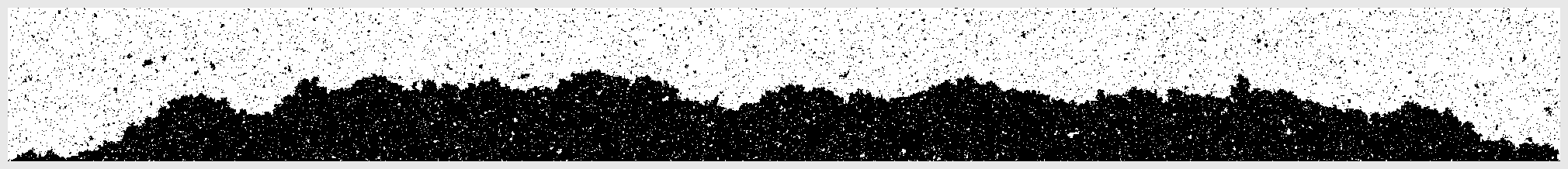
Complete wetting ($h\geq h_{\mathrm{w}}$)

Figure 2. Two-dimensional Ising model at $\beta=0.5$; $+$ spins are white, $-$ spins black. Top: partial wetting regime ($h=0.3$). Bottom: complete wetting regime ($h=1$).

• Partial wetting: When $h\in[0,h_{\mathrm{w}})$, the Hausdorff distance between $\gamma$ and the line $\mathcal{L}\stackrel{{\scriptstyle\text{\tiny{\rm def}}}}{{=}}\left\{x=(x_{1},x_{2})\in\mathbb{R}^{2}\,:\,x_{2}=-\tfrac{1}{2}\right\}$ is of order $\log n$. More precisely, the diameter of the maximal connected components of $\gamma\setminus\mathcal{L}$ have exponential tails (see Fig. 3); this follows from a combination of the methods in [63, 64] and [35].

  

  Figure 3. Typical realizations of the interface of the two-dimensional Ising model in the partial wetting regime can be split into pieces included in disjoint triangles with their basis on the wall. The length of the basis of these triangles has exponential tail.

• Complete wetting: If $h\geq h_{\mathrm{w}}$, the Hausdorff distance between $\gamma$ and the line $\mathcal{L}$ is of order $n^{1/2}$. More precisely, it is expected that, under diffusive scaling, $\gamma$ converges to a Brownian excursion when $h>h_{\mathrm{w}}$; this should follow from a combination of the methods in [64, 18, 39, 17]. Moreover, on the basis of a similar result for the corresponding effective interface model in [28], it is natural to conjecture that the scaling limit is a modulus of Brownian bridge when $h=h_{\mathrm{w}}$.

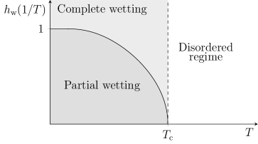
Figure 4. The graph of the critical boundary coupling constant $h_{\mathrm{w}}(\beta)$ as a function of the temperature $T=1/\beta$, in the two-dimensional Ising model. The regime of partial, respectively complete, wetting correspond to the dark, respectively light, shaded area. For $T\geq T_{\mathrm{c}}$, there is no phase coexistence.

Remarkably, $h_{\mathrm{w}}$ can be determined explicitly in this case [1]: it is given by the unique nonnegative solution (see Figure 4) to

$$\exp(2\beta)\bigl{(}\cosh(2\beta)-\cosh(2\beta h_{\mathrm{w}})\bigr{)}=\sinh(2\beta).$$

The sudden change in the behavior of $\gamma$ as $h$ crosses the value $h_{\mathrm{w}}$ is the manifestation of the wetting transition in this setting.

2.1.3. The three-dimensional case.

The current understanding of the wetting transition in the three-dimensional Ising model is much more rudimentary. This is mainly due to the fact that random lines are easier to describe than random surfaces. But more is true: the qualitative behavior is substantially more complicated in the three-dimensional model, as explained below.

One first complication when $d=3$ is the conjectured existence of a roughening transition. Namely, it is well known [31] that, at sufficiently low temperature, imposing boundary conditions that induce the presence of a horizontal interface between $+$ and $-$ bulk phases results in an interface that is rigid: the latter coincides with a perfect plane, apart from rare local deviations. It is conjectured that this interface loses its rigid character at a temperature $\beta_{\rm r}<\beta_{\mathrm{c}}(3)$. This problem remains completely open from a mathematical point of view, only the regime of very low temperatures being well understood. As a consequence, all the results discussed below are valid only at sufficiently large values of $\beta$; in particular, $\beta>\beta_{\rm r}$.

Let us review what is known rigorously about the wetting transition in this model. First, the existence of a value $h_{\mathrm{w}}(\beta)$ separating regimes of partial and complete wetting has been proved in [37]. Moreover, explicit lower and upper bounds on $h_{\mathrm{w}}(\beta)$ have been derived in this work (in particular, $h_{\mathrm{w}}(\beta)\leq 1$ for all $\beta$), and a weak form of localization, resp. delocalization, of the corresponding Peierls contour in the partial wetting, resp. complete wetting, regime was established.

It is however expected that the situation is actually more interesting in this case: inside the partial wetting regime, it is conjectured that there is an infinite sequence of first-order phase transitions, known as layering transitions, at which the microscopic height of the (rigid) interface increases by one unit. The precise behavior is not known, but some (not all fully rigorous) quantitative information about the location of the first few lines has been obtained in [6, 7, 4].

Rigorous results on layering transitions in the context of effective SOS models were obtained in [5], see a discussion in the end of Subsection 4.1.1 below.

2.1.4. Some terminology

Before briefly presenting alternative equivalent characterizations of the wetting transition, we need some terminology, which will also be useful later.

Surface tension.

The free energy per unit-area (unit-length when $d=2$) associated to a linear interface is measured by the surface tension. In the $d$-dimensional Ising model, the latter quantity can be defined as follows. Let $\Lambda_{n}=\{-n,\ldots,n\}^{d}$ and let $\boldsymbol{v}$ be a unit-length vector in $\mathbb{R}^{d}$. Let also $\mathbb{H}^{d}_{\boldsymbol{v},+}\stackrel{{\scriptstyle\text{\tiny{\rm def}}}}{{=}}\left\{i\in\mathbb{Z}^{d}\,:\,i\cdot\boldsymbol{v}\geq 0\right\}$ and $\mathbb{H}^{d}_{\boldsymbol{v},-}\stackrel{{\scriptstyle\text{\tiny{\rm def}}}}{{=}}\mathbb{Z}^{d}\setminus\mathbb{H}^{d}_{\boldsymbol{v},+}$ be the two half-spaces delimited by the plane going though the origin and with normal $\boldsymbol{v}$, and set

$$\Omega^{\boldsymbol{v}}_{n}\stackrel{{\scriptstyle\text{\tiny{\rm def}}}}{{=}}\bigl{\{}\sigma\in\{\pm 1\}^{\mathbb{Z}^{d}}\,:\,\sigma_{i}=\mathbf{1}_{\{i\in\mathbb{H}^{d}_{\boldsymbol{v},+}\}}-\mathbf{1}_{\{i\in\mathbb{H}^{d}_{\boldsymbol{v},-}\}}\text{ for all }i\not\in\Lambda_{n}\bigr{\}}$$

and $\Omega^{+}_{n}\stackrel{{\scriptstyle\text{\tiny{\rm def}}}}{{=}}\bigl{\{}\sigma\in\{\pm 1\}^{\mathbb{Z}^{d}}\,:\,\sigma_{i}=1\text{ for all }i\not\in\Lambda_{n}\bigr{\}}$. The surface tension per unit-area in the direction normal to $\boldsymbol{v}$ is defined by

$$\tau_{\beta}(\boldsymbol{v})\stackrel{{\scriptstyle\text{\tiny{\rm def}}}}{{=}}\lim_{n\to\infty}-\frac{1}{\beta|A_{n}(\boldsymbol{v})|}\log\frac{\mathsf{Z}^{\boldsymbol{v}}_{\Lambda_{n};\beta}}{\mathsf{Z}^{+}_{\Lambda_{n};\beta}},$$ (4)

where $|A_{n}(\boldsymbol{v})|$ is the area (more precisely, the $(d-1)$-dimensional Hausdorff measure) of the set $\left\{x\in[-n,n]^{d}\,:\,x\cdot\boldsymbol{v}=0\right\}$ and, for $\star\in\{+,\boldsymbol{v}\}$,

$$\mathsf{Z}^{\star}_{\Lambda_{n};\beta}\stackrel{{\scriptstyle\text{\tiny{\rm def}}}}{{=}}\sum_{\sigma\in\Omega^{\star}_{n}}\exp\bigl{\{}\beta\sum_{\{i,j\}\cap\Lambda_{n}\neq\varnothing}\sigma_{i}\sigma_{j}\bigr{\}}.$$

The existence of the limit in the definition of $\tau_{\beta}(\boldsymbol{v})$ is proved in [58]. The function $\tau_{\beta}$ can be extended to $\mathbb{R}^{d}$ by positive homogeneity. Namely, one sets $\tau_{\beta}(0)\stackrel{{\scriptstyle\text{\tiny{\rm def}}}}{{=}}0$ and, for any $0\neq x\in\mathbb{R}^{d}$, $\tau_{\beta}(x)\stackrel{{\scriptstyle\text{\tiny{\rm def}}}}{{=}}\tau_{\beta}(x/\|x\|_{\scriptscriptstyle 2})\|x\|_{\scriptscriptstyle 2}$. This function can be shown to be convex [58]. Moreover, one can show [14, 56] that $\tau_{\beta}$ is an order parameter in the sense that $\tau_{\beta}>0$ if and only if $\beta>\beta_{\mathrm{c}}(d)$.

Equilibrium crystal shapes (Wulff shapes) associated to the surface tension $\tau_{\beta}$ are described in Appendix A.

In the three-dimensional Ising model at sufficiently low temperature (that is, at sufficiently large values of $\beta$), it is possible to prove that the surface tension $\tau_{\beta}(\boldsymbol{v})$ does not behave smoothly as a function of $\boldsymbol{v}$. Namely, parameterizing $\boldsymbol{v}$ as a function of the polar angle $\theta$ and azimuthal angle $\varphi$, we can write $\tau_{\beta}(\theta,\varphi)\equiv\tau_{\beta}(\boldsymbol{v}(\theta,\varphi))$. It is then possible to prove that $\partial\tau_{\beta}(\theta,\varphi)/\partial\theta$ is discontinuous at $\theta=0$ for all $\varphi$. This has an impact on the geometry of the Wulff shape, which develops facets (that is, flat portions of positive two-dimensional Hausdorff measure) orthogonally to each lattice direction. These facets are conjectured to disappear at the roughening transition. Proofs and additional information on these issues can be found in [59]. Note that it is still an open problem to determine whether these macroscopically flat pieces of the Wulff shape are actually also microscopically flat (in the same sense as the Dobrushin interface). We will see later, in Section 4, what can be said about that in the simpler context of effective interface models.

Wall free energy.

We now want to introduce a quantity measuring the free energy per unit-area associated to an interface along a substrate. The definition is very similar to that of the surface tension: the wall free energy is defined by

$$\tau^{\small\mathrm{bd}}_{\beta,h}\stackrel{{\scriptstyle\text{\tiny{\rm def}}}}{{=}}\lim_{n\to\infty}-\frac{1}{(2n)^{d-1}}\log\frac{\mathsf{Z}^{-}_{\Delta_{n};\beta,h}}{\mathsf{Z}^{\pm}_{\Delta_{n};\beta,h}}.$$

Existence of the limit is proved in [36].

2.1.5. Alternative characterizations of the wetting transition.

We now briefly present some alternative characterizations of the wetting transition (a more detailed discussion can be found in the review [62] and in the papers [36, 37]).

• Surface Gibbs states: It can be shown [36, 37] that complete wetting occurs if and only if there is a unique surface Gibbs state, that is, if and only if $\lim_{n\to\infty}\mu^{-}_{n;\beta,h}=\lim_{n\to\infty}\mu^{\pm}_{n;\beta,h}$.

• Thermodynamics: It can be shown [36, 37] that $\tau_{\beta}(\boldsymbol{e}_{d})\geq\tau^{\small\mathrm{bd}}_{\beta,h}$ for all $\beta$ and $h$, and that partial wetting occurs if and only if $\tau_{\beta}(\boldsymbol{e}_{d})>\tau^{\small\mathrm{bd}}_{\beta,h}$.

• Canonical ensemble: Here, one considers the measure $\mu^{-}_{\Delta_{n};\beta,h}$ conditioned on a fixed value of the magnetization in $\Delta_{n}$: $\sum_{i\in\Delta_{n}}\sigma_{i}=m|\Delta_{n}|$. When $|m|$ is strictly smaller than the spontaneous magnetization $m^{*}(\beta)$, the system reacts by creating a droplet of $+$ phase immersed in a background of $-$ phase. This droplet has a deterministic macroscopic shape, given by the solution of a suitable generalization of the variational problem (VP) in Appendix A, the so called Winterbottom problem  [9]. It can then be shown [63, 10] that, at least on the level of the variational problem, the resulting droplet attaches itself to the bottom wall if and only if $|h|<h_{\mathrm{w}}(\beta)$

3. Critical prewetting

As we have just described, wetting phenomena occur at phase coexistence: the bulk of the system is occupied by some thermodynamically stable phase $A$, while the substrate favors another stable phase $B$, resulting, in the regime of complete wetting, in the creation of a mesoscopic layer of phase $B$ covering the substrate.

When the system is brought away from phase coexistence, phase $B$ becomes thermodynamically unstable and the wetting transition disappears: irrespectively of the preference of the substrate towards “phase” $B$, the latter never forms a mesoscopic layer. Nevertheless, there is still a trace of the wetting transition, at least as the system is brought close to phase coexistence. Namely, when this happens, a microscopic layer of the unstable phase $B$ covers the substrate, and the width of this layer diverges as the system approaches phase coexistence if, and only if, the system at phase coexistence is in the complete wetting regime. This phenomenon is known as prewetting and takes different forms in two- and three-dimensional models.

3.1. Critical prewetting in the Ising model

In order to discuss prewetting in the Ising model, we need to modify the Hamiltonian in order to bring the system away from phase coexistence. The most natural way to do that is by adding a positive bulk magnetic field, the latter ensuring that only the $+$ phase is thermodynamically stable. Namely, we consider the following modification of the Hamiltonian in (2): for $\lambda\geq 0$, let

$$\mathcal{H}_{n;h,\lambda}(\sigma)\stackrel{{\scriptstyle\text{\tiny{\rm def}}}}{{=}}\mathcal{H}_{n;h}(\sigma)-\lambda\sum_{i\in\Delta_{n}}\sigma_{i}.$$ (5)

We denote by $\mu^{\pm}_{\Delta_{n};\beta,h,\lambda}$ the corresponding Gibbs measure on $\Omega^{\pm}_{\Delta_{n}}$. Clearly, the latter reduces to $\mu^{\pm}_{\Delta_{n};\beta,h}$ when $\lambda=0$. In this section, we assume that $h\geq h_{\mathrm{w}}(\beta)$, that is, the system is in the complete wetting regime when $\lambda=0$.

3.1.1. The two-dimensional case

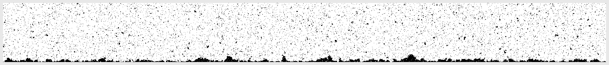
$\lambda=0.01$

$\lambda=0.001$

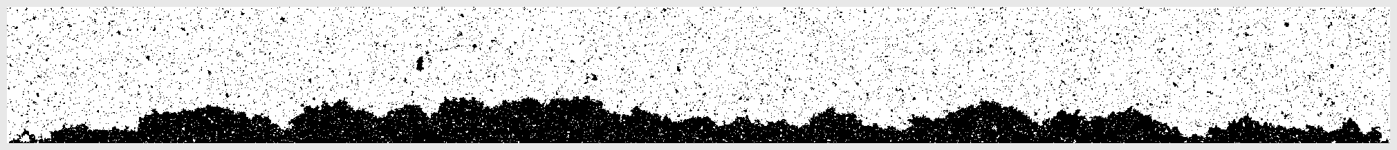
$\lambda=0.0001$

Figure 5. Two-dimensional Ising model at $\beta=0.5$; $+$ spins are white, $-$ spins black. Layer of unstable $-$ phase covering the substrate in the complete wetting regime ($h=1$), for decreasing values of the bulk field $\lambda$.

In order to analyze prewetting in this model, we have to provide a suitable definition for the (average) thickness of the layer of unstable $-$ phase. One possible choice is to define the latter as

$$w(\lambda;\beta,h)\stackrel{{\scriptstyle\text{\tiny{\rm def}}}}{{=}}\lim_{n\to\infty}(2n+1)^{-1}\,|\mathrm{below}(\gamma)|,$$

where $|\mathrm{below}(\gamma)|$ denotes the area of the region of $\mathbb{R}^{2}$ delimited by the unique infinite Peierls contour $\gamma$ and the line $\mathcal{L}$. We can now state the following

Conjecture 3.1.

For any $\beta>\beta_{\mathrm{c}}(2)$ and any $h\geq h_{\mathrm{w}}(\beta)$, there exist constants $c_{1}>0$, $c_{2}<\infty$ and $\lambda_{0}>0$ such that, for all $\lambda<\lambda_{0}$,

$$c_{1}\lambda^{-1/3}\leq w(\lambda;\beta,h)\leq c_{2}\lambda^{-1/3}.$$

We refer the reader to [69] for some partial results toward proving this conjecture.

The continuous divergence of the thickness of the unstable film as $\lambda\downarrow 0$ is characteristic of critical prewetting. In fact, one has a precise conjecture for the process describing the properly scaled interface in the limit $\lambda\downarrow 0$. Namely, as explained above, the typical width of the layer if of order $\lambda^{-1/3}$. It is also possible to argue that the natural horizontal lengthscale is of order $\lambda^{-2/3}$. So, one might hope that after rescaling the interface by $\lambda^{1/3}$ vertically and by $\lambda^{2/3}$ horizontally, the resulting process might be described by some universal scaling limit. That this occurs was actually established for a class of one-dimensional effective interface models in [48]. Let us describe the conjectured result for the Ising model.

Given a particular realization of the Ising interface $\gamma$, let us denote by $\sigma_{\gamma}$ the configuration in $\Omega_{\Delta_{n}}^{\pm}$ which has $\gamma$ as its unique contour. We can then define the upper and lower “envelopes” $\gamma^{\pm}:\mathbb{Z}\to\mathbb{Z}$ of $\gamma$ by

$$\gamma^{+}(i)\stackrel{{\scriptstyle\text{\tiny{\rm def}}}}{{=}}\max\left\{j\in\mathbb{Z}\,:\,\sigma_{(i,j)}(\omega_{\gamma})=-1\right\}+1,$$

$$\gamma^{-}(i)\stackrel{{\scriptstyle\text{\tiny{\rm def}}}}{{=}}\min\left\{j\in\mathbb{Z}\,:\,\sigma_{(i,j)}(\omega_{\gamma})=+1\right\}-1.$$

Note that $\gamma^{+}(i)>\gamma^{-}(i)$ for all $i\in\mathbb{Z}$. Using the random-walk representation of Ising interfaces, described in more detail in Section 4.3 , one can prove that, with probability close to $1$, $\gamma^{-}$ and $\gamma^{+}$ remain very close to each other: there exists $K=K(\beta)<\infty$ such that, with probability tending to $1$ as $n\to\infty$,

$$\max_{|i|\leq R}|\gamma^{+}(i)-\gamma^{-}(i)|\leq K\log R.$$ (6)

for any $R>0$. Let us now introduce the rescaled profiles $\hat{\gamma}^{\pm}:[-1,1]\to\mathbb{R}$. Given $y=(y_{1},y_{2})\in\mathbb{R}^{2}$, let us write $\lfloor y\rfloor\stackrel{{\scriptstyle\Delta}}{{=}}(\lfloor y_{1}\rfloor,\lfloor y_{2}\rfloor)$. We then set, for any $x\in\mathbb{R}$,

$$\hat{\gamma}^{+}_{\lambda}(x)=\lambda^{1/3}\gamma^{+}(\lfloor\lambda^{-2/3}x\rfloor),$$

and similarly for $\gamma^{-}$. Thanks to (6), for any $c\geq 0$,

$$\lim_{\lambda\downarrow 0}\lim_{n\to\infty}\mu^{\pm}_{\Delta_{n};\beta,h,\lambda}\bigl{(}\sup_{|x|\leq\lambda^{-c}}|\hat{\gamma}^{+}_{\lambda}(x)-\hat{\gamma}^{-}_{\lambda}(x)|<\epsilon\bigr{)}=1,\quad\forall\epsilon>0,$$

so that in order to analyze the scaling limit of $\gamma$, it is sufficient to understand the scaling limit of, say, $\gamma^{+}$.

Conjecture 3.2.

In the limit $n\to\infty$, followed by $\lambda\downarrow 0$, the distribution of $\hat{\gamma}^{+}_{\lambda}$ under $\mu^{\pm}_{\Delta_{n};\beta,h,\lambda}$ converges weakly to that of a Ferrari–Spohn diffusion with parameters $\sigma^{2}=\chi_{\beta}$ and $q(r)=2m^{*}r$ (see Appendix B), where $\chi_{\beta}=\left(\tau_{\beta}(0)+\tau_{\beta}^{\prime\prime}(0)\right)^{-1}$ is the curvature of the unnormalized equilibrium crystal shape $\mathcal{W}_{\beta}$ in lattice directions $\pm\mathsf{e}_{i}$ and $m^{*}=m^{*}(\beta)\stackrel{{\scriptstyle\Delta}}{{=}}\lim_{n\to\infty}\mu^{+}_{\Lambda_{n};\beta}(\sigma_{0})$ is the spontaneous magnetization.

Recall that Wulff shape are defined and discussed in Appendix A. In Appendix C we try to justify the above conjecture by sketching an argument for proving a similar statement in the context of self-avoiding walks under area tilts.

3.1.2. The three-dimensional case.

As mentioned above, infinitely many layering transitions are conjectured to occur in the partial wetting regime in this case. Not surprisingly, this has also consequences for the prewetting behavior: namely, as the bulk field $\lambda$ is decreased towards zero, the continuous divergence observed in the two-dimensional model is replaced by an infinite sequence of first-order phase transitions, also known as layering transitions. The latter are however much better understood rigorously than the corresponding transitions in the absence of a bulk external field.

The existence of the first such layering transition was established, at low temperatures, in [37].

Moreover, in the case $h=1$, it was argued in [6, 7] that, there is a decreasing sequence $(\lambda(n))_{n\geq 0}$ such that $\lim_{n\to\infty}\lambda(n)=0$ and

• for each $n\geq 0$, when $\lambda\in(\lambda(n),\lambda(n+1))$, the film of unstable $-$ phase has a thickness of $n$ microscopic layers (with a microscopically sharply-defined boundary);

• at the transition points $\lambda=\lambda(n)$, there is a coexistence of two Gibbs states with layers of thickness $n-1$ and $n$.

In addition, some information on the location of the first few lines can be found in these papers. In principle, delocalization and scaling of these top level lines as the bulk field $\lambda$ goes to zero, should bear resemblance to critical prewetting of Ising interfaces in two dimensions.

3.1.3. Relation to metastability

In this section, we describe a different setup in which a closely related phenomenon occurs. We consider only the two-dimensional Ising model in the box $\Lambda_{n}=\{-n,\dots,n\}^{2}$ with $-$ boundary condition and the Hamiltonian (5), but something similar occurs also in higher dimensions. We will be interested in the behavior of this model when $h=1$ and $\lambda>0$. That is, we consider the Gibbs measure $\mu^{-}_{\Lambda_{n};\beta,1,\lambda}$.

As before, because of the presence of a positive bulk field $\lambda$, the $+$ phase is the unique equilibrium phase. Now, however, the boundary condition favors $-$ spins, which leads to delicate metastability issues. Namely, two types of behavior could be expected: either the boundary condition dominates and the box is filled with the $-$ phase, or the bulk field dominates and the box is occupied by the $+$ phase (except, possibly, close to the boundary). Replacing the $-$ phase inside the box by the $+$ phase yields an energetic gain of order $\lambda|\Lambda_{n}|$ due to preference of the bulk field for the $+$ phase, but there is also an energetic cost of order $|\partial\Lambda_{n}|$ associated to the boundary of the “droplet” of $+$ phase thus created. One would thus expect that the transition between these two regimes should occur for a value of $\lambda$ of order $1/n$. This is indeed the case.

More precisely, the following is proved in [65]: Let $\mathsf{W}_{\beta}$ be the unit area Wulff shape for the surface tension $\tau_{\beta}$, precisely as specified in Appendix A. Let $\nu_{\beta}$ be the critical slope for the dual constrained variational problem (DCVP), see formula (93). Let

$$B_{0}(\beta)\stackrel{{\scriptstyle\text{\tiny{\rm def}}}}{{=}}\frac{1}{2m^{*}(\beta)}\nu_{\beta}=\frac{4\tau_{\beta}(\mathsf{e})+\tau_{\beta}(\mathsf{W}_{\beta})}{8m^{*}_{\beta}}.$$ (7)

Then, for all $\beta>\beta_{\mathrm{c}}(2)$, there exists $K(\beta)<\infty$ such that the following holds:

• Let $B<B_{0}(\beta)$ and set $\lambda=\lambda(n)=B/n$. Then, as $n\to\infty$, with probability going to $1$, all Peierls contours are of diameter at most $K(\beta)\log n$ .

• Let $B>B_{0}(\beta)$ and set $\lambda=\lambda(n)=B/n$. Define $\nu=2m^{*}(\beta)B>\nu_{\beta}$, and let $\mathsf{a}=\mathsf{a}(\beta,\nu)$ be the corresponding solution of (DCVP), and $\mathsf{P}^{\mathsf{a}}_{\beta}$ be the corresponding Wulff plaquette.
  Then, for any $\epsilon>0$, the following occurs with probability going to $1$ as $n\to\infty$ (see Figure 6): There is a unique Peierls contour of diameter more than $K(\beta)\log n$ and this contour is contained in the set $(1+\epsilon)n\mathsf{P}^{a}_{\beta}$ and surrounds the set $(1-\epsilon)n\mathsf{P}^{a}_{\beta}$.

Figure 6. The two-dimensional Ising model at $\beta=0.48$ in $\Lambda_{1000}$ with $-$ boundary condition and a bulk magnetic field $\lambda=0.007$.

Therefore, in the regime $B>B_{0}(\beta)$, there are macroscopic interfaces along (part of) the four walls. As before, these interfaces coincide with the walls only at the macroscopic scale. At the microscopic scale, there is a layer of $-$ phase between the walls and the droplet of $+$ phase. It is conjectured that the width of this layer is of order

$$\lambda(n)^{1/3}\sim n^{-1/3},$$

as $n\to\infty$, in perfect analogy with the discussion of prewetting above. Moreover, the $(n^{2/3},n^{1/3})$-rescaling of Ising interfaces along flat boundaries of the box is expected to lead to Ferrari–Spohn asymptotics as described in Conjecture 3.2.

3.2. Interfacial wetting and prewetting in the 2d Blume–Capel model

The phenomena described above in the two-dimensional Ising model occur of course in a broad class of systems. As one example, we discuss here the two-dimensional Blume–Capel model. The latter has spins taking values in the set {-1,0,1} and a formal Hamiltonian of the form

$$-J\sum_{i\sim j}\sigma_{i}\sigma_{j}-\lambda\sum_{i}\sigma_{i}^{2}.$$

It is well known [15] that, at sufficiently low temperatures, there exists $\lambda_{c}=\lambda_{c}(\beta)>0$ such that, for all $\lambda<\lambda_{c}$, there exists a unique extremal translation-invariant Gibbs state, typical configurations of which are composed of an infinite “sea” of $0$ spins with only finite “islands”. In contrast, for all $\lambda>\lambda_{c}$, there are exactly two extremal translation-invariant Gibbs states with “seas” of $+$, respectively $-$ spins. Finally, at the triple point $\lambda_{c}$, all three measures coexist (and are the only extremal translation-invariant states).

Let us consider the model in the box $\Lambda_{n}$ with a boundary condition made up of $+$ spins in the upper half plane, and $-$ spins in the lower half plane. Assume first that $\lambda=\lambda_{c}$. Then, as in the Ising model, this boundary condition favors $+$ spins in the top half of the box and $-$ spins in the bottom half, with an interface separating the two regions. However, now a new phenomenon occurs. Let us denote by $\tau^{+-}$ the surface tension associated to the interface between the $+$ and $-$ phases, and define similarly $\tau^{+0}$ and $\tau^{-0}$. It is expected that $\tau^{+-}=\tau^{+0}+\tau^{-0}$ and that this relation should imply that it is preferable for the system to introduce a mesoscopic layer of $0$ phase between the regions occupied by the $+$ and $-$ spins. The width of this layer should be of order $\sqrt{n}$. No rigorous results seem to have been obtained on this problem, but a discussion can be found in [13].

Let us now assume that $\lambda>\lambda_{c}$. In this case, the layer of $0$ phase becomes unstable and, similarly to what we saw for prewetting, it becomes microscopic. One can then once more analyze how the width of this layer changes as $\lambda\downarrow\lambda_{c}$. The natural conjecture, supported by numerical simulations (see [66] for the earliest we could find), is that it should again behave as $\lambda^{1/3}$, which suggests a Ferrari–Spohn structure of appropriate scaling limits. Again, none of the above has yet been established, although some related results have been obtained far away from the triple point, $\lambda\gg\lambda_{c}$ [41].

4. Effective interface models

The discrete two-dimensional effective interface models discussed in this section are defined over lattice boxes $\Lambda_{N}\subset\mathbb{Z}^{2}$,

$$\Lambda_{N}=\{-N,-N+1,\dots,N-1,N\}^{2},$$ (8)

$N$ being the linear size of the system. The interface is described as the set of integer random heights $\varphi=\{\varphi_{x}\}_{x\in\mathbb{Z}^{2}}$. Thus, $\varphi_{0}$ describes the random height of the interface at the center of the box $\Lambda_{N}$.

Unless mentioned otherwise we shall assume that the interfaces in question are pinned at zero height outside $\Lambda_{N}$; $\varphi_{x}=0$ if $x\not\in\Lambda_{N}$.

The passage from the Ising model with boundary conditions (3) to the effective interface models considered in this Section can be viewed either as a strong interaction limit, in which the coupling constants $J_{i,j}$ in (2) are set to $+\infty$ for vertical bonds $(i,j)$, or as a simplification of “true” Ising interfaces obtained by prohibiting overhangs. The former point of view gives rise to the class of Solid-on-Solid (SOS) models specified in Subsection 4.1.1 below. The latter point of view still leaves room for incorporating low-temperature phases above and below the interface. An effective model of this sort is discussed in Subsection 4.1.2.

4.1. Low-temperature interfaces and ensembles of level lines

At low temperatures, the large-scale properties of effective interfaces should be recovered from the statistics of large level lines which locally look like one-dimensional effective random walks.

4.1.1. SOS-type models

The Hamiltonian $\mathcal{H}_{N}$ and the probability distribution $\mathbb{P}_{N}^{\beta}$ are given by

$$-\mathcal{H}_{N}(\varphi)=\sum_{xy}J_{xy}U(\varphi_{x}-\varphi_{y})+\sum_{x}f(\varphi_{x})\quad\text{ and }\quad\mathbb{P}_{N}^{\beta}(\underline{\varphi})=\frac{1}{Z_{N}}{\rm e}^{-\beta\mathcal{H}_{N}(\underline{\varphi})},$$ (9)

where $Z_{N}=Z_{N}(\beta,V,J,f)$ is the partition function. Familiar examples in the case of nearest-neighbor interactions, $J_{xy}=\mathbbm{1}_{x\sim y}$, and identically zero self-potential, $f\equiv 0$, include:

1. SOS model if $U(t)=\left|t\right|$.

2. Discrete Gaussian (DG) surface if $U(t)=|t|^{2}$.

3. Restricted SOS model in the case of $U(t)=\left|t\right|+\infty\cdot\mathbbm{1}_{\left|t\right|>1}$.

Below, we shall restrict attention to (a), but other potentials should be kept in mind.

The self-interaction $f$ is used to model external influences, such as bulk fields, interaction with a substrate or a hard-wall constraint. Consider, for instance,

$$f(\varphi)=-\infty\cdot\mathbf{1}_{\{\varphi<0\}}-\lambda\varphi+h\,\mathbf{1}_{\{\varphi=0\}}.$$ (10)

The first term forces the surface to stay above the wall: $\varphi_{x}\geq 0\;\forall x$. If we use (9) to model a random interface between coexisting phases, then the parameter $\lambda$ measures the strength of the bulk magnetic field, while $h$ measures the interaction between the interface and a substrate placed at zero height.

Random interfaces modeled with Hamiltonians as in (9) display a rich phenomenology.

Roughening.

Let $f\equiv 0$. It is well known (and not difficult to prove) that $\mathbb{E}_{N}^{\beta}{\left|\varphi_{0}\right|}$ is bounded uniformly in $N$ when $\beta$ is large, for both the SOS and DG models. Groundbreaking results by Fröhlich and Spencer [38] imply that there is a roughening transition for both models. Namely, $\lim_{N\to\infty}\mathbb{E}_{N}^{\beta}{\left|\varphi_{x}-\varphi_{0}\right|^{2}}\geq c\log|x|$. The result is proved by a mapping to a Coulomb gas; finding a direct probabilistic argument and deriving a (presumably Gaussian) scaling limit are well-known challenges.

Entropic repulsion.

Let $f(\varphi)=-\infty\cdot\mathbf{1}_{\{\varphi<0\}}$. Early results [12, 54] imply that the interface, as the size $N$ of the system grows, is always repelled to infinity, even in the case of large $\beta$ for which the unconstrained interface is localized.

In the context of SOS models, the lower temperature (that is, $\beta\gg 1$) situation was analyzed in much more detail in the recent works [21, 20, 22]. Their results include sharp height concentration (on a diverging level $\sim\log N$), macroscopic scaling limit for level sets, and $N^{1/3}$ bounds on fluctuations of level lines long the flat segments of the boundary $\partial\Lambda_{N}$. Furthermore, height concentration results (but not macroscopic scaling limits and approximate order of fluctuations of level lines) were established for low-temperature models with more general interactions of the form $U(t)=\left|t\right|^{p}\;p\in(1,\infty]$ in [57].

Prewetting and Layering.

Let $f(\varphi)=-\lambda\varphi-\infty\cdot\mathbf{1}_{\{\varphi<0\}}$. The bulk field $\lambda$ penalizes large values of the volume below the surface; in this sense, it models the bulk magnetic field in (5). When $\lambda>0$, there is a competition between the entropic repulsion and the volume penalization imposed by $\lambda$. In the low-temperature regime, this results is an infinite sequence of first-order phase transitions, which can be characterized in terms of the concentration of the typical interface height at increasing values: $1,2,3,\dots$; see [29, 23, 55] for precise statements of the results. Roughly speaking, it was proved that for any sufficiently large $\beta$ there exists a number $n_{{\rm max}}(\beta)$ and a sequence of bulk fields $\lambda_{0}(\beta)>\lambda_{1}(\beta)>\dots>\lambda_{n_{\rm max}}(\beta)$, such that the surface is concentrated on height $n$ whenever

$$\lambda\in\left(\lambda_{n}(\beta),\lambda_{n-1}(\beta)\right).$$ (11)

It is not clear whether the restriction $n\leq n_{{\rm max}}$ is of a technical nature or not. Presumably it is not, and prewetting thus occurs as $\lambda\downarrow 0$ through an infinite sequence of jumps of the typical interface height.

Wetting.

Let $f(\varphi)=h\,\mathbf{1}_{\{\varphi=0\}}-\infty\cdot\mathbf{1}_{\{\varphi<0\}}$. The boundary field $h$ plays the same role as in (1). There is now a competition between entropic repulsion and attraction by the substrate (measured through $h$). Define the dry set $\mathcal{A}_{N}=\left\{x\in\Lambda_{N}\,:\,\varphi_{x}=0\right\}$. For SOS interfaces, it was proved in [24] that typically $|\mathcal{A}_{N}|\sim N^{2}$ when $h$ is large, while $|\mathcal{A}_{N}|\ll N^{2}$, when $h>0$ is small. More precisely, it is proven in [24] that the dry set has a uniformly (in the linear size of the system $N$) positive density if

$$\beta h>-\log\Bigl{(}\frac{1-{\rm e}^{-\beta}}{16(1+{\rm e}^{\beta})}\Bigr{)},$$ (12)

whereas the density of the dry set vanishes ($|\mathcal{A}_{N}|$ being at most of order $N$), as $N\to\infty$, as soon as

$$\beta h<-\log(1-{\rm e}^{-4\beta}).$$ (13)

This is a perturbative result, which does not directly address the nature of transition for $h$-s between the two values in (12) and (13).

The lower temperature situation was analyzed in much more detail in [5], where the existence of a sequence of layering transitions has been established and explained. Roughly speaking, the following is shown (see Theorem 1.1 in [5] for the precise statement). Fix $\epsilon>0$. Then, for any given $n\in\mathbb{N}$ and for all $\beta$ sufficiently large, the surface concentrates on height $n$ whenever

$$-\ln\left(1-{\rm e}^{-4\beta}\right)+(2+\epsilon){\rm e}^{-2\beta(n+3)}\leq h\beta\leq-\ln\left(1-{\rm e}^{-4\beta}\right)+(2-\epsilon){\rm e}^{-2\beta(n+2)}.$$ (14)

Such a result had previously been stated, but not proved, in [12].

Finally, we note a recent preprint [52] which contains (Theorem 2.1 there) an identification of the right hand side of (13) as the low temperature wetting transition threshold and, furthermore, contains a claim on an almost piece-wise affine structure which bears a strong indication of an infinite sequence of layering transitions. A proof and a comprehensive analysis of such infinite sequence of layering transitions appeared (Theorems 2.1 and 2.6 there) in a very recent sequel [53] to [52]. We have not checked the arguments of [52, 53] in detail. If correct (which is presumably the case) they fetch a complete, modulo a certain analyticity issue - see Remark 2.2. in [53], original description of layering transition driven by boundary fields in the SOS context.

4.1.2. SOS-type model coupled to a bulk field

The interfaces have the same distribution as in (9), with $f\equiv 0$. Instead of the latter, consider a coupling with high- and low-density bulk Bernoulli fields below and, respectively, above the interface. These fields are designed to mimic co-existing low- and high- density phases, say vapor and solid, in lattice gases. Namely, consider a three-dimensional vessel

$$B_{N}=\Lambda_{N}\times\{-N+\tfrac{1}{2},\ldots,N-\tfrac{1}{2}\}.$$

A realization of $\varphi$ (constrained to stay inside $B_{N}$) splits $B_{N}$ into two halves; $B_{N}=S_{N}(\underline{\varphi})\cup V_{N}(\underline{\varphi})$. Given $0<p_{\rm v}<p_{{\rm s}}<1$, we place particles with probability $p_{{\rm s}}$ into sites of $S_{N}$ and with probability $p_{\rm v}$ into sites of $V_{N}$. We use $\mathbb{Q}_{N}$ to denote the distribution of the resulting triple $(\varphi,\eta^{{\rm s}},\eta^{{\rm v}})$. That is,

$$\mathbb{Q}_{N}^{\beta}(\varphi,\eta^{{\rm s}},\eta^{{\rm v}})\propto{\rm e}^{-\beta\mathcal{H}_{N}(\varphi)}\mathbb{B}_{S_{N}(\underline{\varphi})}^{p_{{\rm s}}}(\eta^{{\rm s}})\mathbb{B}_{V_{N}(\underline{\varphi})}^{p_{{\rm v}}}(\eta^{{\rm v}}),$$ (15)

where $\mathbb{B}^{p}_{A}$ is the $p$-Bernoulli product measure on $\{0,1\}^{A}$.

Faceting.

The measure (15) does not incorporate a bulk chemical potential, a hard wall or the interaction with an active substrate. However, the layering phenomenon can be modeled in the following way: Note that the average number of particles under $\mathbb{Q}_{N}^{\beta}$ is $(p_{{\rm s}}+p_{{\rm v}})N\left|\Lambda_{N}\right|\stackrel{{\scriptstyle\Delta}}{{=}}r_{N}N^{3}$. At low temperatures, the interface is flat. Facets of macroscopic size appear under the canonical constraint

$$\mathbb{Q}_{N,\mathsf{a}}^{\beta}(\cdot)=\mathbb{Q}_{N}^{\beta}\bigl{(}\,\cdot\bigm{|}\sum_{{\mathsf{z}}\in S_{N}}\eta^{\rm s}_{\mathsf{z}}+\sum_{{\mathsf{z}}\in V_{N}}\eta^{{\rm v}}=\lfloor r_{N}N^{3}+\mathsf{a}N^{2}\rfloor\bigr{)}.$$ (16)

The model in (15), for the SOS interaction $U(t)=\left|t\right|$, was introduced in [45], where it was established that first-order phase transitions under the canonical measure (16) occur (as the parameter $a$ grows), corresponding to the creation of the first two facets. Actually the forthcoming work [46] implies that the model undergoes an infinite sequence of such first-order layering transitions. The discontinuity of facet sizes at critical values of $a$ is due to the coupling with the bulk Bernoulli field, in a way similar to the spontaneous creation of a droplet in the 2D Ising model [8]. Presumably, coupling of an SOS interface with bulk Bernoulli fields reflects in a more accurate way the faceting of microscopic Wulff crystals in the low-temperature 3D Ising model, which was the motivation for an earlier study of the phenomenon in the context of pure SOS models in [11].

4.1.3. Level lines of low temperature interfaces

Random interfaces under either (9) or (15) can be described in terms of their level lines. Since the surface is pinned at zero height outside $\Lambda_{N}$, level lines are closed microscopic contours. It is convenient to employ north-east splitting rules to avoid ambiguities at vertices which are incident to four edges, see for instance [47, Subsection 2.1] or [20, Definition 2.1]. In the sequel we shall tacitly assume that such rules are employed and, consequently, we shall talk about compatible portions of level lines or contours without further comments.

Given a contour $\gamma$, we use $\left|\gamma\right|$ to denote its length, $\mathrm{diam}(\gamma)$ to denote its diameter in $\|\cdot\|_{\infty}$-norm, $\mathring{\gamma}$ to denote its interior and $\mathsf{A}=\mathsf{A}(\gamma)$ to denote the area of $\mathring{\gamma}$. Fix $\epsilon>0$ sufficiently small. If $N$ is the linear size of the system, a microscopic contour $\gamma$ is said to be large if $\mathrm{diam}(\gamma)\geq\epsilon N$ and small if $\mathrm{diam}(\gamma)\leq\epsilon^{-1}\log N$. Otherwise, it is said to be intermediate.

In the case of low-temperature SOS ($U(t)=\left|t\right|$) Hamiltonians, contour weights factorize and cluster expansions were derived and explored, see for instance [30, 29, 23, 60, 45, 5, 21, 20, 47]. It is natural to make expansions relative to the unconstrained SOS model (with $f\equiv 0$). In all situations of interest, one should in principle be able to rule out intermediate contours and check that there is at most one ordered stack

$$\underline{\gamma}=\{\gamma_{1},\ldots,\gamma_{n}\}\text{ satisfying }\mathring{\gamma}_{1}\subseteq\mathring{\gamma}_{2}\subseteq\cdots\subseteq\mathring{\gamma}_{n}\subseteq\Lambda_{N}$$ (17)

of compatible large microscopic contours. A somewhat simplified version of the SOS polymer weights $q_{\beta,N}(\underline{\gamma})$ that are obtained via cluster expansions with respect to small contours reads as:

$$\log q_{\beta,N}(\underline{\gamma})=-\beta\sum\left|\gamma_{i}\right|+\sum_{i}\sum_{\mathcal{C}}\Phi_{\beta,N}(\mathcal{C};\gamma_{i})+\Psi_{\beta,N}(\underline{\gamma})+F_{\beta,N}(\mathsf{A}_{1},\mathsf{A}_{2},\ldots).$$ (18)

Above $\Phi_{\beta,N}(\mathcal{C};\gamma)$ are the cluster weights for the model defined on a finite box $\Lambda_{N}$; in particular, $\Phi_{\beta,N}$ incorporates the effects due to the finite geometry of the latter, including short-range (exponential tails) interactions with the boundary $\partial\Lambda_{N}$. $\Psi_{N,\beta}$ is a multi-body short-range (again in the sense of exponential decay with $\mathrm{diam}(\mathcal{C})$) interaction between the different contours in a stack, which reflects the possibility of sharing clusters. $F_{\beta,N}$ takes different forms in different models. Let us provide some examples.

SOS model coupled to a bulk Bernoulli field

Under (16), the function $F_{\beta,N}$ takes, up to $\log N$-corrections, the following form:

$$F_{\beta,N}(\mathsf{A}_{1},\mathsf{A}_{2},\ldots)=-\frac{(\mathsf{a}N^{2}-\sum_{i}\mathsf{A}_{i})^{2}}{2D\left|B_{N}\right|},$$ (19)

where $D=\tfrac{1}{2}\{p_{\rm s}(1-p_{\rm s})+p_{\rm v}(1-p_{\rm v})\}$. It should be clear where (19) is coming from: The volume of the surface $\varphi$ with the prescribed collection $\underline{\gamma}$ of large microscopic contours should concentrate around $\mathsf{A}_{1}+\dots+\mathsf{A}_{n}$. The excess number of particles is $\mathsf{a}N^{2}-\sum_{1}^{n}\mathsf{A}_{i}$, as imposed by the canonical constraint in (16), and it should be compensated by fluctuations of the density of the Bernoulli fields above and below the surface. The latter have an average variance $D$ per site.

For the Hamiltonians (9), (10), the $\mathbb{Z}$-symmetry of infinite-volume states is broken and there are different values of metastable free energies, which one computes using restricted contour ensembles, $f^{*}_{m}=f^{*}_{m}(\beta,\lambda,h)$ for interfaces living on heights $m\in\mathbb{N}_{0}$. Accordingly, the expression for $F_{\beta,N}$ should take into account these metastable free energies. Let us write it down up to lower-order terms for surfaces which are represented by ordered stacks (17). For such a surface, the total area of the interface at height $m=0,\dots,n$

$$\begin{cases}\mathsf{A}_{1},\qquad\qquad&\text{if $m=n$,}\\ \mathsf{A}_{2}-\mathsf{A}_{1}&\text{if $m=n-1$,}\\ \vdots&\\ \left|\Lambda_{N}\right|-\mathsf{A}_{n}&\text{if $m=0.$}\end{cases}$$ (20)

Hence,

$$F_{\beta,N}(\mathsf{A}_{1},\mathsf{A}_{2}, \dots,\mathsf{A}_{n})$$

$$=f^{*}_{n}\mathsf{A}_{1}+f^{*}_{n-1}(\mathsf{A}_{2}-\mathsf{A}_{1})+f^{*}_{n-2}(\mathsf{A}_{3}-\mathsf{A}_{2})+\dots+f_{0}^{*}(\left|\Lambda_{N}\right|-\mathsf{A}_{n})$$

$$=\sum_{\ell=1}^{n}(f_{n-\ell+1}^{*}-f^{*}_{n-\ell})\mathsf{A}_{\ell}+f^{*}_{0}\left|\Lambda_{N}\right|\stackrel{{\scriptstyle\Delta}}{{=}}\sum_{\ell=1}^{n}r^{*}_{n-\ell+1}\mathsf{A}_{\ell}+f^{*}_{0}\left|\Lambda_{N}\right|.$$ (21)

Entropic repulsion

In the case of a pure hard-wall constraint, $f(\varphi)=-\infty\cdot\mathbf{1}_{\{\varphi<0\}}$, it was established in [20] (see (1.6) in the latter paper) that (again up to lower-order terms) free energies $f_{m}^{*}$ and, accordingly, area tilts $r^{*}_{m}$ are of the form

$$f_{m}^{*}=-c_{\beta}{\rm e}^{-4\beta(m+1)}\quad{\rm and}\quad r^{*}_{m}=c_{\beta}{\rm e}^{-4\beta m}\left(1-{\rm e}^{-4\beta}\right).$$ (22)

Consequently,

$$F_{\beta,N}(\mathsf{A}_{1},\mathsf{A}_{2},\ldots,\mathsf{A}_{n})=\bar{c}_{\beta}\sum_{\ell=1}^{n}{\rm e}^{-4\beta(n-\ell+1)}A_{\ell}+f^{*}_{0}\left|\Lambda_{N}\right|.$$ (23)

where we have set $\bar{c}_{\beta}=c_{\beta}\left(1-{\rm e}^{-4\beta}\right)$. By Lemma 2.4 in [20] the limit $\lim_{\beta\to\infty}\bar{c}_{\beta}=1$.

Bulk magnetic field.

In the case of pure entropic repulsion, the area tilts $r^{*}_{\ell}$ in (22) are always positive. In the presence of bulk field, $f(\varphi)=-\lambda\,\varphi-\infty\cdot\mathbf{1}_{\{\varphi<0\}}$, the situation is different. Roughly speaking, it is shown in [23] (see Theorem 4.1 there for the precise statement) that $r^{*}_{n}$ is positive as long as $\lambda<\lambda_{n-1}(\beta)$, see (11). This means that, on the level of resolution suggested by (18) there could be at most

$$\bar{n}=\bar{n}(\beta,\lambda)=\max\left\{n\,:\,\lambda\leq\lambda_{n-1}(\beta)\right\}$$ (24)

large contours in the stack (17), and, accordingly, we should restrict attention to

$$F_{\beta,N}(\mathsf{A}_{1},\mathsf{A}_{2},\ldots)=\sum_{1}^{\bar{n}}r_{\bar{n}-\ell+1}\mathsf{A}_{\ell}+f^{*}_{0}\left|\Lambda_{N}\right|.$$ (25)

Boundary magnetic fields.

The case $f(\varphi)=-\infty\cdot\mathbf{1}_{\{\varphi<0\}}+h\mathbbm{1}_{\varphi=0}$ is even more complicated. Indeed, (14) is based on Proposition 3.2 in [5], which indicates that the area tilt $r^{*}_{n}$ is positive as long as

$$\beta h\leq-\ln\left(1-{\rm e}^{-4\beta}\right)+(2-\epsilon){\rm e}^{-2\beta(n+2)}.$$ (26)

This means that, as in the case of bulk field, one should restrict attention to a finite number $\bar{n}(\beta,h)$ of large contours in the stack (17).

4.2. Variational problems and macroscopic scaling limits.

In order to discuss the macroscopic scaling limits of large microscopic level lines for the $2+1$ dimensional surfaces we consider here, we need to introduce the notion of two-dimensional inverse correlation length , as well as of Wulff shapes and Wulff plaquettes, which are related to the low-temperature massive structure of these level lines.

4.2.1. Inverse correlation length

For low-temperature polymers with infinite-volume weights

$$\log q_{\beta}^{\sf f}(\gamma)=-\beta\left|\gamma\right|+\sum_{\mathcal{C}}\Phi_{\beta}(\mathcal{C};\gamma),$$ (27)

the inverse correlation length $\xi_{\beta}$ is well defined; see, e.g., [45, 20] or [47, Subsection 2.2]. Specifically, for ${\mathsf{x}}\in\mathbb{Z}^{2}$, set $q_{\beta}^{\sf f}({\mathsf{x}})=\sum_{\gamma:0\to{\mathsf{x}}}q_{\beta}^{\sf f}(\gamma)$. Then, given a direction $\mathfrak{n}\in\mathbb{S}^{1}$,

$$\xi_{\beta}(\mathfrak{n})=-\lim_{M\to\infty}\frac{1}{M}\log q_{\beta}^{\sf f}(\lfloor M\mathfrak{n}\rfloor).$$ (28)

Finally, $\xi_{\beta}$ extends to $\mathbb{R}^{2}$ by homogeneity. More details on the existence and properties of the limit in (28) can be found in Subsection 4.3.1 below. Note that, for the models we consider, the cluster weights in (27), and hence the inverse correlation length $\xi_{\beta}$, inherit the symmetries of $\mathbb{Z}^{2}$.

4.2.2. Multi-layer constrained macroscopic variational problems

The relevant notions of (two-dimensional) Wulff shape and Wulff plaquettes are introduced in Appendix A. Given an area $\mathsf{b}\leq 4$, let $\xi_{\beta}(\mathsf{b})$ be the minimal surface energy over subsets of $[-1,1]^{2}$ of area $\mathsf{b}$. In other words, $\xi_{\beta}(\mathsf{b})$ is given by (86) if $\mathsf{b}\in[0,w_{\beta}]$ and, accordingly, by (88) if $\mathsf{b}\in[w_{\beta},4]$. Assuming that the expression for the contour weights in (18) can be approximated by $\sum_{i=1}^{n}\log q_{\beta}^{\sf f}(\gamma_{i})$, that is, assuming that, at low temperatures, finite-volume effects and the interaction between different contours in the stack can be ignored, we conclude that information on the macroscopic scaling (by the linear system size $N$) of the stack of large contours should in principle be read from the constrained macroscopic variational problem

(MCVP)  $\max_{\mathsf{a}_{1}\leq\mathsf{a}_{2}\leq\cdots\leq 4}\bigl{\{}-\sum_{i}\xi_{\beta}(\mathsf{a}_{i})+\frac{1}{N}F_{\beta,N}(N^{2}\mathsf{a}_{1},N^{2}\mathsf{a}_{2},\ldots)\bigr{\}}$ .

Let us explore this variational problem for a class of examples we consider here.

SOS model coupled to a bulk Bernoulli field

The multi-layer constrained variational problem (MCVP) was completely worked out in [46] for $F_{\beta,N}$ of the form (19), that is when

$$\frac{1}{N}F_{\beta,N}(N^{2}\mathsf{a}_{1},N^{2}\mathsf{a}_{2},\ldots)=-\frac{(\mathsf{a}-\sum_{i}\mathsf{a}_{i})^{2}}{16D}.$$

In this case, the variation problem (MCVP) becomes

$$\min_{\mathsf{a}_{1}\leq\mathsf{a}_{2}\leq\ldots\leq 4}\Bigr{\{}\sum_{i}\xi_{\beta}(\mathsf{a}_{i})+\frac{(\mathsf{a}-\sum_{i}\mathsf{a}_{i})^{2}}{16D}\Bigr{\}}.$$ (29)

Of course, there are different solutions for different values of $\mathsf{a}$. It is proven in [46] that (29) undergoes an infinite sequence of first-order phase transitions in the following sense: There exists a sequence $0=\mathsf{b}_{0}<\mathsf{b}_{1}<\mathsf{b}_{2}<\ldots$, with $\lim_{k\to\infty}\mathsf{b}_{k}=\infty$, such that there is a unique solution to (29), for any $\ell$ and for any $\mathsf{a}\in(\mathsf{b}_{\ell},\mathsf{b}_{\ell+1})$. Furthermore, this solution contains exactly $\ell$ shapes

$$\mathsf{S}_{1}\subseteq\mathsf{S}_{2}=\mathsf{S}_{3}=\cdots=\mathsf{S}_{\ell},$$ (30)

and $\mathsf{S}_{2},\ldots,\mathsf{S}_{\ell}$ are Wulff plaquettes, whereas $\mathsf{S}_{1}$ is either a Wulff plaquette identical to $\mathsf{S}_{i}$, $i\geq 2$, or it is a Wulff shape of the same radius as $\mathsf{S}_{i}$, $i\geq 2$. Moreover, starting from $\ell^{*}=\ell^{*}(\beta)$, the optimal solutions contain only Wulff plaquettes.

Entropic repulsion

Consider the expression (23) for $F_{N,\beta}$ (with the term $f^{*}_{0}\left|\Lambda_{N}\right|$ dropped), applied to the microscopic areas $\mathsf{A}_{k}=N^{2}\mathsf{a}_{k}$:

$$F_{N,\beta}(N^{2}\mathsf{a}_{1},\ldots,N^{2}\mathsf{a}_{n})=\bar{c}_{\beta}\sum_{k=1}^{n}{\rm e}^{-4\beta(n+1-k)}N^{2}\mathsf{a}_{k}=\bar{c}_{\beta}N\sum_{k=1}^{n}{\rm e}^{-4\beta(n+1-k)}N\mathsf{a}_{k}.$$ (31)

The corresponding surface tension is $N\sum_{k=1}^{n}\xi_{\beta}(\mathsf{a}_{k})$. This means that the top layer (of area $N^{2}\mathsf{a}_{1}$) might appear only if

$$\max_{\mathsf{a}_{1}\leq 4}\left\{\bar{c}_{\beta}{\rm e}^{-4\beta n}N\mathsf{a}_{1}-\xi_{\beta}(\mathsf{a}_{1})\right\}\geq 0.$$

This falls into the framework of the dual constrained variational problem (DCVP) discussed in Appendix A.

Going back to (31), we conclude that the number of layers $n^{*}$ should satisfy

$$\nu_{\beta}\in\bigl{(}\bar{c}_{\beta}{\rm e}^{-4\beta(n^{*}+1)}N,\bar{c}_{\beta}{\rm e}^{-4\beta n^{*}}N\bigr{)}.$$ (32)

Accordingly, define $\nu^{1}=\bar{c}_{\beta}{\rm e}^{-4\beta n^{*}}N$ and

$$\nu^{k}={\rm e}^{4\beta(k-1)}\nu^{1}\text{, for $k=2,3,\ldots$},$$ (33)

and consider the Wulff plaquettes

$$\mathsf{P}_{\beta}^{\mathsf{b}_{1}}\subset\mathsf{P}_{\beta}^{\mathsf{b}_{2}}\subset\cdots\text{ where }\mathsf{b}_{k}=\mathsf{a}(\beta,\nu^{k})=\mathrm{argmax}_{\mathsf{a}\in[0,4]}\bigl{\{}\nu^{k}\mathsf{a}-\xi_{\beta}(\mathsf{a})\bigr{\}}.$$ (34)

Bulk magnetic field

Consider (18) and (25). Recall that there are at most $\bar{n}$ contours in a stack. Restricting attention to contours with total length bounded above by $KN$, we infer that, for all $\beta$ large enough,

$$\beta\sum_{i=1}^{\bar{n}}\left|\gamma_{i}\right|-\sum_{i=1}^{\bar{n}}\sum_{\mathcal{C}}\Phi_{\beta,N}(\mathcal{C};\gamma_{i})-\Psi_{\beta,N}(\underline{\gamma})\leq\bar{n}(K+1)N\beta.$$

Hence,

$$\log q_{\beta,N}(\underline{\gamma})\geq\sum_{\ell=1}^{\bar{n}}\left(r^{*}_{n-\ell+1}N^{2}\mathsf{a}_{\ell}-N(K+1)\beta\right).$$ (35)

This means that if $r^{*}_{\bar{n}}>0$, the inner-most contour $\gamma_{1}$ tends to fill in the whole box: $\mathsf{a}_{1}\to 4$, as $N\to\infty$. In other words, modulo a difficult and, as we mentioned, still partially open question of characterization of $\bar{n}=\bar{n}(\beta,\lambda)$, the limiting variational problem in the case of a fixed bulk field $\lambda>0$ is somewhat trivial - all $\bar{n}$ limiting shapes are full $[-1,1]^{2}$ squares.

A more interesting situation should occur if the bulk field $\lambda=\lambda_{N}$ tends to zero as $N\to\infty$, but for the moment even a reliable conjecture along these lines seems to be beyond reach.

Boundary magnetic fields.

The situation with the limiting macroscopic variational problem in the case of boundary fields is somewhat similar to that in the bulk field. Namely, modulo an incomplete characterization of the typical, as $N\to\infty$, number of layers $\bar{n}(\beta,h)$, the limiting variational problem seems to be a trivial one.

4.2.3. Macroscopic scaling limits

All the results below are discussed under the tacit assumption that the inverse temperature $\beta$ is large enough.

Let us first consider SOS-type effective interface models with $\mathbb{P}_{N}^{\beta}$ as defined in (9).

Entropic repulsion

In the case of entropic repulsion, the scaling limits of large level lines were completely worked out in [20]. Let us formulate a particular instance of their results for sequences of side-lengths $N_{\ell}$ satisfying (recall (32) which determines $n^{*}=n^{*}(N)$)

$$\lim_{\ell\to\infty}\bar{c}_{\beta}{\rm e}^{-4\beta n^{*}(N_{\ell})}N_{\ell}=\nu^{1}>\nu_{\beta},$$ (36)

where $\nu_{\beta}$ is the critical value for the variational problem (DCVP).

Theorem 4.1.

Assume (36). Let $\{\gamma_{1},\gamma_{2},\ldots\}$ be the ordered stack of large contours as in (17). Then, using ${\rm d}_{\mathsf{H}}$ for the Hausdorff distance,

$$\lim_{\ell\to\infty}\mathbb{P}_{N_{\ell}}^{\beta}\Bigl{(}{\rm d}_{\mathsf{H}}\bigl{(}\frac{\gamma_{k}}{N_{\ell}},\partial\mathsf{P}_{\beta}^{\mathsf{b}_{k}}\bigr{)}>\epsilon\Bigr{)}=0,$$ (37)

for any $k\in\mathbb{N}$ fixed and any $\epsilon>0$, where $\mathsf{b}_{k}=\mathsf{a}(\beta,\nu^{k})$ with $\nu^{k}$ defined as in (33), and $\mathsf{P}_{\beta}^{\mathsf{b}_{k}}$ are optimal Wulff plaquettes as in (34).

SOS models with bulk and boundary fields

Formula (35) indicates that the following should happen for $\beta$ large enough:

$$\lim_{N\to\infty}\mathbb{P}_{N_{\ell}}^{\beta}\Bigl{(}{\rm d}_{\mathsf{H}}\bigl{(}\frac{\gamma_{1}}{N},\partial[-1,1]^{2}\bigr{)}>\epsilon\Bigr{)}=0,$$ (38)

for any $\epsilon>0$.

Presumably, such results could be deduced from [29, 23, 55] for the range of $\beta$ and $\lambda$ to which the results of the latter papers apply.

The same is true regarding boundary fields in the regime in which the results of [5] apply.

More interesting phenomena might appear if one allows $\lambda_{N}\to\infty$ or $h_{N}\to\infty$ as the linear size $N$ of the system grows, but a rigorous analysis will presumably require going well beyond the existing techniques.

Facets in the SOS model coupled with bulk Bernoulli fields

The scaling limits for large level lines under the measure $\mathbb{Q}_{N,\mathsf{a}}^{\beta}$ defined in (16) are studied in [46]. For the moment, the results there are formulated contingent to a proof of predominance of repulsion between different contours in a stack over weak interaction between these contours, as described in more detail in Subsection 4.3.2 below. This issue was overlooked in [45]. Here is the conjectured statement:

Theorem 4.2.

There exists $\beta_{0}$ large enough such that the following holds: Fix $\beta>\beta_{0}$ and $\ell\in\mathbb{N}$. Let $\mathsf{a}\in(\mathsf{b}_{\ell},\mathsf{b}_{\ell+1})$, where the sequence $\mathsf{b}_{1},\mathsf{b}_{2},\ldots$ is the one appearing in the solution of the variational problem (29). Then,

$$\lim_{N\to\infty}\mathbb{Q}_{N,\mathsf{a}}^{\beta}(\text{Exactly one stack of $\ell$ large contours})=1.$$ (39)

Furthermore, let $\mathsf{S}_{1},\ldots,\mathsf{S}_{\ell}$ be the optimal shapes as in (30). Then, for any $\epsilon>0$ fixed, the unique $\ell$-stack $\{\gamma_{1},\ldots,\gamma_{\ell}\}$ satisfies:

$$\lim_{N\to\infty}\mathbb{Q}_{N,\mathsf{a}}^{\beta}\Bigl{(}\max_{1\leq k\leq\ell}{\rm d}_{\mathsf{H}}\bigl{(}\frac{\gamma_{k}}{N},\partial\mathsf{S}_{k}\bigr{)}>\epsilon\Bigr{)}=0.$$ (40)

The results of [47] justify the conclusion in the initial case of the first facet ($\mathsf{b}_{1}<\mathsf{a}<\mathsf{b}_{2}$) as they imply that the interaction with the boundary of $\Lambda_{N}$ does not modify the surface tension.

4.3. Structure and fluctuations of interacting level lines

The macroscopic level lines are nested stacks of closed contours. A careful analysis of large-scale fluctuations of such stacks under the probability distribution with unnormalized weights (18) should involve several steps:

STEP 1. One should develop a fluctuation theory of mesoscopic segments of a single large contour. At this stage, the inverse correlation length $\xi_{\beta}$ is incorporated and the effective local one-dimensional random walk structure of level lines is uncovered.

STEP 2. One should develop a procedure, usually known as skeleton calculus, to patch mesoscopic segments into a single closed macroscopic contour.

STEP 3. Different macroscopic contours in a nested stack are subject to entropic repulsion. One should check that the entropic repulsion prevails over the weak attraction due to the cluster sharing terms $\Psi_{\beta,N}$ in (18). In particular, the interaction between different contours should not modify the surface tension. Note that the multi-layer constrained variational problem (MCVP) is stated under the tacit assumption that this indeed does not happen.

STEP 4. Finally, one should understand what are the proper scaling regimes (as the size $N$ of the system goes to $\infty$) corresponding to the fluctuations of the level lines under various area-type tilts $F_{\beta,N}$.

In the sequel we discuss what is known and what is not known along these lines.

4.3.1. Ising polymers and effective random walk representation

Let us discuss the low-temperature weights (27) for a mesoscopic segment $\gamma$ of a single level line. This is a model of low-temperature Ising polymers and we shall closely follow the exposition in the recent work [47]; in particular, we shall refer to Subsections 2 and 3 of the latter paper for missing details.

The low-temperature assumption comes into play through the very possibility to perform cluster expansions leading to (27), and it is further quantified in terms of exponential decay properties of the cluster weights $\Phi_{\beta}(\mathcal{C};\gamma)$. Namely, assume that there exist some $\chi>0$ such that, for all $\beta$ sufficiently large,

$$\bigl{|}\Phi(\mathcal{C},\gamma)\bigr{|}<\exp\bigl{\{}-\chi\beta(\mathrm{diam}(\mathcal{C})+1)\bigr{\}}.$$ (41)

Under (41), the polymer weights $q^{\mathsf{f}}_{\beta}(\gamma)$ in (27) can be rewritten in the following form (see [47, Subsection 3.2]):

$$q^{\mathsf{f}}_{\beta}(\gamma)=\sum_{\underline{\mathcal{C}}}{\rm e}^{-(\beta+c(\beta))\left|\gamma\right|}\prod_{i}\rho_{\beta}(\mathcal{C}_{i},\gamma)\stackrel{{\scriptstyle\Delta}}{{=}}\sum_{\underline{\mathcal{C}}}\rho^{\mathsf{f}}_{{\beta}}\bigl{(}[\gamma,\underline{\mathcal{C}}]\bigr{)}.$$ (42)

Above, the summation is with respect to all finite collections of connected clusters $\underline{\mathcal{C}}=\{\mathcal{C}_{i}\}$. The modified inverse temperature $\beta+c(\beta)$ is slightly larger than the original one: $0<c(\beta)<{\rm e}^{-\chi\beta}$. Finally, the product cluster weights $\rho_{\beta}(\mathcal{C},\gamma)$ are non-negative and exponentially decaying:

$$0\leq\rho_{\beta}(\mathcal{C},\gamma)\leq{\rm e}^{-\chi\beta(\mathrm{diam}(\mathcal{C})+1)}\mathbf{1}_{\{\text{$\mathcal{C}$ is incompatible with $\gamma$}\}}.$$ (43)

The weights $\rho_{\beta}(\mathcal{C},\gamma)$ are translation invariant. In such circumstances, a straightforward adjustment of sub-additivity arguments implies that the limit in (28) exists for all $\beta$ sufficiently large, and that the corresponding surface tension $\xi_{\beta}$ is strictly positive and convex.

Furthermore, much sharper results hold: Let us call couples $\mathfrak{a}=[\gamma,\underline{\mathcal{C}}]$ animals. Given a cone $\mathcal{Y}$ and a point ${\mathsf{x}}\in\gamma=({\mathsf{x}}_{0},\ldots,{\mathsf{x}}_{n})$, let us say that ${\mathsf{x}}$ is a $\mathcal{Y}$-break point of $[\gamma,\underline{\mathcal{C}}]$ if it is an interior point of $\gamma$ (that is, ${\mathsf{x}}\in\{{\mathsf{x}}_{1},\ldots.{\mathsf{x}}_{n-1}\}$) and the following holds:

$$\{{\mathsf{x}}_{0},\ldots,{\mathsf{x}}_{i}\}\subset({\mathsf{x}}-\mathcal{Y}),\quad\{{\mathsf{x}}_{i},\ldots,{\mathsf{x}}_{n}\}\subset({\mathsf{x}}+\mathcal{Y})\text{ and }\cup_{i}\mathcal{C}_{i}\subset({\mathsf{x}}-\mathcal{Y})\cup({\mathsf{x}}+\mathcal{Y}).$$ (44)

Evidently, if ${\mathsf{x}}$ is a $\mathcal{Y}$-break point of an animal $[\gamma,\underline{\mathcal{C}}]$, then we can represent it as a concatenation

$$\mathfrak{a}=[\gamma,\underline{\mathcal{C}}]=[\gamma^{1},\underline{\mathcal{C}}^{1}]\circ[\gamma^{2},\underline{\mathcal{C}}^{2}]=\mathfrak{a}^{1}\circ\mathfrak{a}^{2}$$

such that $\gamma^{1},\underline{\mathcal{C}}^{1}\subset({\mathsf{x}}-\mathcal{Y})$ and $\gamma^{2},\underline{\mathcal{C}}^{2}\subset({\mathsf{x}}+\mathcal{Y})$.

Definition 1.

Given a cone $\mathcal{Y}$, let us say that an animal $\mathfrak{a}=[\gamma,\underline{\mathcal{C}}]$ with $\gamma=({\mathsf{x}}_{0},{\mathsf{x}}_{1},\ldots,{\mathsf{x}}_{n})$ is $\mathcal{Y}$-irreducible if it does not have break points.

Unnormalized Wulff shapes $\mathcal{W}_{\beta}$ are defined in (82) of Appendix A. With each $\mathsf{h}\in\partial\mathcal{W}_{\beta}$, we can associate a convex cone

$$\mathcal{Y}_{\mathsf{h}}=\left\{{\mathsf{x}}\,:\,\mathsf{h}\cdot{\mathsf{x}}\geq\epsilon\right\}.$$ (45)

We assume that $\epsilon>0$ is sufficiently small, so that $\mathcal{Y}_{\mathsf{h}}$ always contains a lattice direction in its interior (and hence there are paths $\gamma$ which satisfy $\gamma\subset\mathcal{Y}_{\mathsf{h}}$).

Ornstein–Zernike theory

The relevant input from the OZ theory (see for instance [49, Subsections 3.3 and 3.4] and [47, Section 4.1]) can be summarized as follows: For $\mathsf{h}\in\partial\mathcal{W}_{\beta}$, let $\mathcal{Y}_{\mathsf{h}}$ be the cone defined in (45) and let $\mathsf{A}_{\mathsf{h}}$ be the corresponding set of irreducible animals. For $\mathfrak{a}=[\gamma,\underline{\mathcal{C}}]\in\mathsf{A}_{\mathsf{h}}$ with $\gamma=({\mathsf{x}}_{0},\ldots,{\mathsf{x}}_{n})$, define the length $\left|\mathsf{a}\right|=\left|\gamma\right|$ and the displacement $\mathsf{X}(\mathsf{a})={\mathsf{x}}_{n}-{\mathsf{x}}_{0}$, and set (recall (84) and (42))

$$\mathbb{P}_{\beta}^{\mathsf{h}}(\mathfrak{a})={\rm e}^{\mathsf{h}\cdot\mathsf{X}(\mathsf{a})}\rho_{\beta}^{\mathsf{f}}(\mathfrak{a}).$$ (46)

Let us say that an $\mathcal{Y}_{\mathsf{h}}$-irreducible animal is a left diamond, respectively a right diamond, if

$$\gamma\subset({\mathsf{x}}_{n}-\mathcal{Y}),\text{ respectively }\gamma\subset({\mathsf{x}}_{0}+\mathcal{Y}).$$ (47)

An animal $\mathfrak{a}$ is said to be a diamond if it is both a left and a right diamond. We use the notation $\mathsf{D}^{\mathsf{l}}_{\mathsf{h}},\mathsf{D}^{\mathsf{r}}_{\mathsf{h}}$ and $\mathsf{D}_{\mathsf{h}}=\mathsf{D}^{l}_{\mathsf{h}}\cap\mathsf{D}^{r}_{\mathsf{h}}$ for the corresponding sets of animals.

Theorem 4.3.

For all $\beta$ large enough and for every $\mathsf{h}\in\partial\mathcal{W}_{\beta}$, $\mathbb{P}_{\beta}^{\mathsf{h}}$ is a probability distribution on $\mathsf{D}_{\mathsf{h}}$ with exponentially decaying tails on $\mathsf{A}_{\mathsf{h}}$. That is,

$$\sum_{\mathfrak{a}\in\mathsf{D}_{\mathsf{h}}}\mathbb{P}_{\beta}^{\mathsf{h}}(\mathfrak{a})=1\text{ and }\sum_{\mathfrak{a}\in\mathsf{A}_{\mathsf{h}}}\bigl{\{}\mathbb{P}_{\beta}^{\mathsf{h}}(\left|\mathfrak{a}\right|>k)+\mathbb{P}_{\beta}^{\mathsf{h}}(\mathsf{X}(\mathfrak{a})>k)\bigr{\}}<{\rm e}^{-\nu_{\beta}k},$$ (48)

for any $k>1$, where $\nu_{\beta}$ does not depend on $\mathsf{h}$.

Furthermore, $\partial\mathcal{W}_{\beta}$ is locally analytic with uniformly strictly positive curvature . In fact, the parametrization of $\partial\mathcal{W}_{\beta}$ in a neighborhood of $\mathsf{h}$ can be described as

$$\mathsf{g}+\mathsf{h}\in\partial\mathcal{W}_{\beta}\quad\Leftrightarrow\quad\mathbb{E}_{\beta}^{\mathsf{h}}\bigl{(}{\rm e}^{\mathsf{g}\cdot\mathsf{X}(\mathfrak{a})}\bigr{)}=1.$$ (49)

In particular, $\xi_{\beta}$ is differentiable at any ${\mathsf{x}}\neq 0$ and

$$\mathsf{h}_{\mathsf{x}}=\nabla\xi_{\beta}({\mathsf{x}})$$ (50)

is the unique point on $\partial\mathcal{W}_{\beta}$ satisfying $\mathsf{h}_{\mathsf{x}}\cdot{\mathsf{x}}=\max_{\mathsf{h}\in\partial\mathsf{K}_{\beta}}\mathsf{h}\cdot{\mathsf{x}}=\xi_{\beta}({\mathsf{x}})$.

Theorem 4.3 indicates that a typical mesoscopic segment of a level line should look like a one-dimensional necklace of irreducible animals. Let us make this precise.

Effective RW representation of mesoscopic segments of level lines

Let ${\mathsf{x}}$ be a distant point and consider the set of all animals $\mathfrak{a}=[\gamma,\underline{\mathcal{C}}]$ from the origin to ${\mathsf{x}}$. In other words, consider the set of all animals $\mathsf{a}$ with $\mathsf{X}(\mathfrak{a})={\mathsf{x}}$.

Now, (28) implies that $q^{\mathsf{f}}_{\beta}({\mathsf{x}})\asymp{\rm e}^{-\xi_{\beta}({\mathsf{x}})}$. Consider $\mathsf{h}=\mathsf{h}_{\mathsf{x}}$ as defined in (50). Then,

$$1\asymp{\rm e}^{\xi_{\beta}({\mathsf{x}})}q^{\mathsf{f}}_{\beta}({\mathsf{x}})=\sum_{\mathsf{X}(\mathsf{a})={\mathsf{x}}}{\rm e}^{\mathsf{h}\cdot\mathsf{X}(\mathsf{a})}\rho_{\beta}^{\mathsf{f}}(\mathfrak{a}).$$

By (46) and (48), and up to corrections of order ${\rm e}^{-\nu_{\beta}\|{\mathsf{x}}\|}$, we can restrict attention to animals $\mathfrak{a}$ of the form

$$\mathfrak{a}=\mathfrak{b}^{\mathsf{l}}\circ\mathfrak{a}^{1}\circ\cdots\circ\mathfrak{a}^{m}\circ\mathfrak{b}^{\mathsf{r}},$$ (51)

with $\mathfrak{b}^{l}\in\mathsf{D}^{l}_{\mathsf{x}}$, $\mathfrak{b}^{r}\in\mathsf{D}^{r}_{\mathsf{h}}$ and $\mathsf{a}^{i}\in\mathsf{D}_{\mathsf{h}}$.

The effective random walk representation, see Figure 7, of mesoscopic segments $\gamma:0\mapsto{\mathsf{x}}$ can be recorded as follows: Let $\mathsf{X}_{1},\mathsf{X}_{2},\ldots$ be i.i.d. $\mathcal{Y}_{\mathsf{h}}$-valued random variables distributed according to $\mathbb{P}_{\beta}$, that is,

$$\mathbb{P}_{\beta}^{\mathsf{h}}(\mathsf{X}_{i}={\mathsf{x}})=\sum_{\begin{subarray}{c}\mathfrak{a}\in\mathsf{D}_{\mathsf{h}}\\ \mathsf{X}(\mathfrak{a})={\mathsf{x}}\end{subarray}}\mathbb{P}_{\beta}^{\mathsf{h}}(\mathfrak{a}).$$ (52)

Set $\mathsf{S}_{j}=\sum_{i=1}^{j}\mathsf{X}_{i}$. Then $\gamma$ is approximated by the polygonal line, or equivalently, the trajectory of the effective random walk through the vertices

$$0,\,\mathsf{X}(\mathfrak{b}^{\mathsf{l}}),\,\mathsf{X}(\mathfrak{b}^{\mathsf{l}})+\mathsf{X}_{1},\ldots,\,\mathsf{X}(\mathfrak{b}^{\mathsf{l}})+\mathsf{S}_{m},\,{\mathsf{x}}.$$

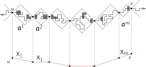
Figure 7. Effective random walk structure of connection between $u$ and $v$.

In this way, the probability distribution of the effective random walk comes from the normalization of the partition function

$${\rm e}^{\xi_{\beta}({\mathsf{x}})}q^{\mathsf{f}}_{\beta}({\mathsf{x}})\bigl{(}1+{\rm o}({\rm e}^{-\nu_{\beta}\|{\mathsf{x}}\|})\bigr{)}=\sum_{\begin{subarray}{c}\mathfrak{b}^{\mathsf{l}}\in\mathsf{D}^{\mathsf{l}}_{\mathsf{h}}\\ \mathfrak{b}^{\mathsf{r}}\in\mathsf{D}^{\mathsf{r}}_{\mathsf{h}}\end{subarray}}\mathbb{P}_{\beta}^{\mathsf{h}}(\mathfrak{b}^{\mathsf{l}})\mathbb{P}_{\beta}^{\mathsf{h}}(\mathfrak{b}^{\mathsf{r}})\sum_{m=1}^{\infty}\otimes\mathbb{P}_{\beta}^{\mathsf{h}}\bigl{(}\mathsf{X}(\mathfrak{b}^{\mathsf{l}})+\mathsf{S}_{m}+\mathsf{X}(\mathfrak{b}^{\mathsf{r}})={\mathsf{x}}\bigr{)}.$$ (53)

The collection of clusters $\underline{\mathcal{C}}$ in $\mathfrak{a}=[\gamma,\underline{\mathcal{C}}]$ should be viewed as hidden variables. The real object of interest are paths $\gamma\stackrel{{\scriptstyle\Delta}}{{=}}\gamma(\mathfrak{a})$. For $\mathfrak{a}\in\mathsf{D}^{\mathsf{l}}_{\mathsf{h}},\mathsf{D}^{\mathsf{r}}_{\mathsf{h}},\mathsf{D}_{\mathsf{h}}$, such paths $\gamma=({\mathsf{x}}_{0},\ldots,{\mathsf{x}}_{n})$ belong, respectively, to the sets $\mathcal{P}^{\mathsf{l}}_{\mathsf{h}}$, $\mathcal{P}^{\mathsf{r}}_{\mathsf{h}}$ and $\mathcal{P}_{\mathsf{h}}=\mathcal{P}^{\mathsf{l}}_{\mathsf{h}}\cap\mathcal{P}^{\mathsf{r}}$, where

$$\mathcal{P}^{\mathsf{l}}_{\mathsf{h}}=\left\{\gamma\,:\,\gamma\subset{\mathsf{x}}_{n}-\mathcal{Y}_{\mathsf{h}}\right\}\text{ and }\mathcal{P}^{\mathsf{r}}_{\mathsf{h}}=\left\{\gamma\,:\,\gamma\subset{\mathsf{x}}_{0}+\mathcal{Y}_{\mathsf{h}}\right\}.$$ (54)

Accordingly, (46) gives rise to a probability distribution on $\mathcal{P}_{\mathsf{h}}$ and to finite measures with exponentially decaying tails on $\mathcal{P}^{\mathsf{l}}_{\mathsf{h}}$ and $\mathcal{P}^{\mathsf{r}}_{\mathsf{h}}$, which we, with a slight abuse of notation, continue to denote $\mathbb{P}_{\beta}^{\mathsf{h}}$. For instance, for $\gamma\in\mathcal{P}_{\mathsf{h}}$,

$$\mathbb{P}_{\beta}^{\mathsf{h}}(\gamma)=\sum_{\mathfrak{a}\,:\,\gamma(\mathfrak{a})=\gamma}\mathbb{P}_{\beta}^{\mathsf{h}}(\mathfrak{a})\mathbf{1}_{\{\mathfrak{a}\in\mathsf{D}_{\mathsf{h}}\}}.$$ (55)

In this way, instead of (51), we can consider

$$\gamma=\eta^{\mathsf{l}}\circ\gamma^{1}\circ\dots\circ\gamma^{m}\circ\eta^{\mathsf{r}}$$ (56)

and, accordingly, instead of (53), we can write

$${\rm e}^{\xi_{\beta}({\mathsf{x}})}q^{\mathsf{f}}_{\beta}({\mathsf{x}})\bigl{(}1+{\rm o}({\rm e}^{-\nu_{\beta}\|{\mathsf{x}}\|})\bigr{)}=\sum_{\begin{subarray}{c}\eta^{\mathsf{l}}\in\mathcal{P}^{\mathsf{l}}_{\mathsf{h}}\\ \eta^{\mathsf{r}}\in\mathcal{P}^{\mathsf{r}}_{\mathsf{h}}\end{subarray}}\mathbb{P}_{\beta}^{\mathsf{h}}(\eta^{\mathsf{l}})\mathbb{P}_{\beta}^{\mathsf{h}}(\eta^{\mathsf{r}})\sum_{m=1}^{\infty}\otimes\mathbb{P}_{\beta}^{\mathsf{h}}\bigl{(}\mathsf{X}(\eta^{\mathsf{l}})+\mathsf{S}_{m}+\mathsf{X}(\eta^{\mathsf{r}})={\mathsf{x}}\bigr{)}.$$ (57)

4.3.2. Skeletons and interaction between different contours

The formula (57) furnishes a probabilistic description of an open “linear” portion $\gamma$ of a level line between two distant points ${\mathsf{x}}$ and ${\mathsf{y}}$. When $\|{\mathsf{y}}-{\mathsf{x}}\|$ is large, it both recovers the macroscopic inverse correlation length $\xi_{\beta}({\mathsf{y}}-{\mathsf{x}})$ and indicates the fluctuation structure of $\gamma$ in the corresponding reduced ensembles. Recall, however, that the microscopic level lines are closed contours of size $N$. The idea of skeleton calculus is to go to an intermediate coarse-graining scale, say $N^{\alpha}$ for $\alpha\in(0,1)$, and try to study closed contours of size $N$ as a concatenation of open paths of size $N^{\alpha}$. This is with a hope that patching such open paths together will lead to controllable corrections to asymptotic formulas such as (57). In the latter case, since the number of different $N^{\alpha}$-skeletons is bounded above by ${\rm e}^{cN^{1-\alpha}}$, one infers concentration near macroscopic shapes of minimal $\xi_{\beta}$-surface energy. We refer to the groundbreaking book [30] where this idea was introduced in the context of the low-temperature 2D Ising model, and to various implementations of skeleton calculus in subsequent works [2, 61, 63, 44, 9, 3, 8, 45].

The implementation of the above procedure should hinge on an argument which would imply that different mesoscopic segments do not interact, in the sense that the total surface energy is the undistorted sum of surface energies over different mesoscopic segments. The same applies if one considers several macroscopic level lines.

Let us elaborate on this problem. Let $\{{\mathsf{x}}_{1},{\mathsf{y}}_{1}\},\ldots,\{{\mathsf{x}}_{k},{\mathsf{y}}_{k}\}$ be a collection of pairs of points in $\mathbb{Z}^{2}$, which represent neighboring vertices of skeletons of the same or different level lines. That is, we assume that $\|{\mathsf{y}}_{j}-{\mathsf{x}}_{j}\|\gg 1$. To fix ideas and in order to avoid redundant notation, let us assume that all ${\mathsf{x}}_{i}$-s lie on a vertical axis through $-\ell\mathsf{e}_{1}$, that is, ${\mathsf{x}}_{i}\cdot\mathsf{e}_{1}\equiv-\ell$, and similarly that ${\mathsf{y}}_{i}$-s lie on a vertical axis through $\ell\mathsf{e}_{1}$. Assume also that these vertices are ordered in the sense that

$${\mathsf{x}}_{1}\cdot\mathsf{e}_{2}\leq{\mathsf{x}}_{2}\cdot\mathsf{e}_{2}\leq\cdots\leq{\mathsf{x}}_{k}\cdot\mathsf{e}_{2},$$

and the same regarding ${\mathsf{y}}_{i}$-s. Let $\underline{\gamma}=(\gamma_{1},\ldots,\gamma_{k})$ be a family of compatible paths $\gamma_{i}:{\mathsf{x}}_{i}\to{\mathsf{y}}_{i}$. Recall that the notion of compatibility comes from the splitting rules employed in the construction of ordered stacks of microscopic level lines as indicated in Subsection 4.1.3. In particular, the $\gamma_{i}$-s do not cross. According to (18) (for the moment, we ignore the confining geometry of $\Lambda_{N}$ as well as the area tilt $F_{\beta,N}$), the free joint weights $\log q_{\beta}^{\mathsf{f}}(\underline{\gamma})$ are given by

$$\log q_{\beta}^{\mathsf{f}}(\underline{\gamma})=-\beta\sum\left|\gamma_{i}\right|+\sum_{i=1}^{k}\sum_{\mathcal{C}}\Phi_{\beta}(\mathcal{C};\gamma_{i})+\Psi_{\beta}(\underline{\gamma})=\sum_{1}^{k}\log q_{\beta}^{\mathsf{f}}(\gamma_{i})+\Psi_{\beta}(\underline{\gamma}),$$ (58)

where the interaction term $\Psi_{\beta}$ is due to overcounting (cluster sharing) and is given by

$$\Psi_{\beta}(\underline{\gamma})=\sum_{\mathcal{C}}\bigl{\{}\Phi_{\beta}(\mathcal{C},\underline{\gamma})-\sum_{1}^{k}\Phi_{\beta}(\mathcal{C};\gamma_{i})\bigr{\}}.$$ (59)

The question is whether one can control the partition functions

$$q_{\beta}^{\mathsf{f}}(\underline{{\mathsf{x}}},\underline{{\mathsf{y}}})\stackrel{{\scriptstyle\Delta}}{{=}}\sum_{\underline{\gamma}\text{ compatible}}q_{\beta}^{\mathsf{f}}(\underline{\gamma})=\sum_{\underline{\gamma}\text{ compatible}}{\rm e}^{\Psi_{\beta}(\underline{\gamma})}\prod_{i=1}^{k}q_{\beta}^{\mathsf{f}}(\gamma_{i})$$ (60)

in terms of $\prod_{i=1}^{k}q_{\beta}^{\mathsf{f}}({\mathsf{y}}_{i}-{\mathsf{x}}_{i})\asymp{\rm e}^{-\sum_{i}\xi_{\beta}({\mathsf{y}}_{i}-{\mathsf{x}}_{i})}$.

Coarse lower bounds are easy: Indeed, by (57), one can confine paths $\gamma_{i}$ to distant tubes, and in the latter case the exponential decay in (41) renders negligible the contribution due to the interaction.

Upper bounds are more difficult. In view of the effective random walk representation (57), the following refined version of the above question makes sense. Consider the partition functions

$$\widehat{q}^{\;\mathsf{f}}_{\beta}(\underline{{\mathsf{x}}},\underline{{\mathsf{y}}})\stackrel{{\scriptstyle\Delta}}{{=}}\sum_{\underline{\gamma}\text{ compatible}}\prod_{i=1}^{k}q_{\beta}^{\mathsf{f}}(\gamma_{i})$$ (61)

and compare the distribution of $\underline{\gamma}$ under $q_{\beta}^{\mathsf{f}}$ with the distribution of $\underline{\gamma}$ under $\widehat{q}^{\;\mathsf{f}}_{\beta}$.

The point is that, under $\hat{q}^{\;\mathsf{f}}_{\beta}$, we are essentially talking about $k$ ordered effective random walks, and the behavior of the latter, including entropic repulsion, is essentially well understood.

The competition between a potential attraction through the $\Psi_{\beta}$ term in (60) and the entropic repulsion between the paths $\gamma_{i}$ is highly non-trivial. It is true that, under (41), the interaction $\Psi_{\beta}$ has an exponential decay of order $\beta$, but so is the variance of effective random walk steps in (52), at least in lattice directions. Furthermore, an additional complication comes with attempts to derive bounds which would hold uniformly up to leading terms in the number of paths $k$.

In fact [47], in the full generality of Ising polymers, just having $\chi>0$ in (41) is not enough to ensure that entropic repulsion wins. The threshold value is conjectured to be $\frac{1}{2}$. In [47], it is shown that, for $\chi>\frac{1}{2}$, a half space polymer which interacts with a hard wall eventually behaves as the free full-space polymer subject to entropic repulsion. An ad hoc counter-example for $\chi=\frac{1}{2}$ is also constructed. A solution to the general question about $k$ interacting paths as stated above is, for the moment, not written down. This issue will be addressed in the forthcoming work [46].

In the case of entropic repulsion [22, 20], upper bounds follow from specific FKG properties of the underlying SOS-Hamiltonians. Namely, for (a slight finite volume modification of) the partition functions $q_{\beta}^{\mathsf{f}}(\underline{{\mathsf{x}}},\underline{{\mathsf{y}}})$ defined in (60), the following holds:

$$q_{\beta}^{\mathsf{f}}(\underline{{\mathsf{x}}},\underline{{\mathsf{y}}})\leq\prod_{i=1}^{k}q_{\beta}^{\mathsf{f}}({\mathsf{y}}_{i}-{\mathsf{x}}_{i}).$$ (62)

4.3.3. Scaling and fluctuations under area tilts

In all the examples discussed in Subsection 4.2.3, the limiting shapes for large level lines are either Wulff shapes or Wulff plaquettes. Actually, in the models we consider, Wulff shapes appear only as top droplets in the case of an SOS surface coupled with Bernoulli bulk fields, and only when the number of facets is bounded by some $\ell^{*}(\beta)$; see the discussion just after (30). In the sequel, we shall consider the fluctuations of large level lines around the limiting plaquettes. The latter contain macroscopic flat segments on the boundary $\partial[-1,1]^{2}$, and we shall focus on the fluctuations of microscopic level lines $\gamma_{1},\gamma_{2},\ldots$ away from these segments.

To fix ideas, let $[-\delta,\delta]\times\{-1\}$ be a flat segment of the top limiting plaquette which appears in either of the scaling limits discussed in Subsection 4.2.3. Then it appears as a flat segment in all the subsequent limiting shapes. Let us zoom in near the microscopic boundary of $\partial\Lambda_{N}$ which contains this segment. We want to study the behavior of microscopic portions $\eta_{1},\eta_{2},\ldots,\eta_{n}$ of the level lines $\gamma_{1},\gamma_{2},\ldots,\gamma_{n}$ above this segment. For the sake of this discussion, we shall consider a somewhat simplified picture along the lines of Subsection 4.3.2.

Let $\{{\mathsf{x}}_{1},{\mathsf{y}}_{1}\},\ldots,\{{\mathsf{x}}_{n},{\mathsf{y}}_{n}\}$ be a collection of pairs of points in the upper half lattice $\mathbb{H}_{+}^{2}=\left\{{\mathsf{x}}\in\mathbb{Z}^{2}\,:\,{\mathsf{x}}\cdot\mathsf{e}_{2}\geq 0\right\}$ such that ${\mathsf{x}}_{i}\cdot\mathsf{e}_{1}\equiv-\delta N$, ${\mathsf{y}}_{i}\cdot\mathsf{e}_{1}\equiv\delta N$ and

$${\mathsf{x}}_{1}\cdot\mathsf{e}_{2}\geq{\mathsf{x}}_{2}\cdot\mathsf{e}_{2}\geq\cdots\geq{\mathsf{x}}_{n}\cdot\mathsf{e}_{2}\geq 0,$$ (63)

with the same vertical ordering holding for ${\mathsf{y}}_{1},\ldots,{\mathsf{y}}_{n}$. Thus, $\underline{{\mathsf{x}}}$ and $\underline{{\mathsf{y}}}$ represent collections of initial and final vertices of ordered portions $\eta_{1},\ldots,\eta_{n}$ of the level lines $\gamma_{1},\ldots,\gamma_{n}$. Let us ignore the interactions between the $\eta_{i}$-s and the remaining pieces of level lines $\gamma_{1}\setminus\eta_{1},\ldots,\gamma_{n}\setminus\eta_{n}$. That is, we assume that the free weights of the paths $\eta_{i}$-s are given by a modification of (58):

$$\log q_{\beta}^{+}(\underline{\eta})=-\beta\sum\left|\eta_{i}\right|+\sum_{i=1}^{k}\sum_{\mathcal{C}\subset\mathbb{H}_{+}^{2}}\Phi_{\beta}(\mathcal{C};\eta_{i})+\Psi_{\beta}^{+}(\underline{\eta})=\sum_{i=1}^{k}\log q_{\beta}^{+}(\eta_{i})+\Psi_{\beta}^{+}(\underline{\eta}),$$ (64)

where the $+$-superscript indicates that we are taking into account the interaction with the boundary of $\Lambda_{N}$. The term $\Psi_{\beta}^{+}(\underline{\eta})$ represents multi-body interactions by cluster sharing between $\eta_{i}$-s, see Figure 8.

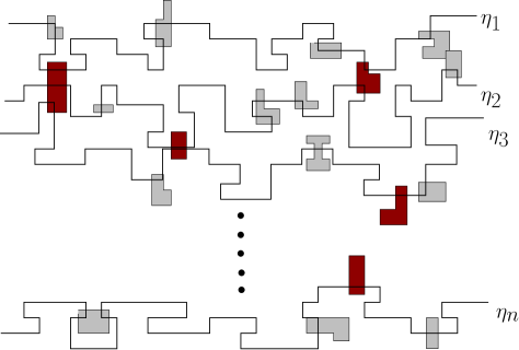
Figure 8. Interaction by cluster sharing between pieces of level lines $\eta_{n},\dots,\eta_{1}$.

The main issue here is to understand what type of corrections one should add to the effective ensemble above in order to incorporate fluctuations away from the rescaled macroscopic limiting shapes. In the sequel, we shall assume that all $\eta_{k}$-s are confined to the strip $[-\delta N,\delta N]\times\mathbb{Z}_{+}$ and use $\mathsf{B}_{k}$ to denote the area below $\eta_{k}$.

SOS model coupled with Bernoulli bulk fields

By assumption, the rescaled optimal limiting plaquettes $N\mathsf{P}^{\mathsf{a}_{1}}_{\beta}=N\mathsf{P}^{\mathsf{a}_{2}}_{\beta}=\cdots=N\mathsf{P}^{\mathsf{a}_{n}}_{\beta}$ of areas $\mathsf{A}_{1}=N^{2}\mathsf{a}_{1},\ldots,\mathsf{A}_{n}=N^{2}\mathsf{a}_{n}$ stick to the boundary of $\partial\Lambda_{N}$ along the segment in question. So, in the rescaled picture of optimal shapes, facets pile up along flat segments of the boundary and $\sum_{k=1}^{n}\mathsf{A}_{k}$ is the optimal total volume below the three-dimensional surface. The level lines $\eta_{1},\ldots,\eta_{n}$ fluctuate away from this flat boundary and, as a result, reduce this optimal volume by $\sum_{k=1}^{n}\mathsf{B}_{k}$. This deficit must be compensated by excess fluctuations of the bulk Bernoulli field. Consider now (19). The excess price is, up to lower-order terms, given by

$$-\frac{(\mathsf{a}N^{2}-\sum_{i}\mathsf{A}_{i})^{2}}{2D\left|B_{N}\right|}+\frac{(\mathsf{a}N^{2}-\sum_{i}\mathsf{A}_{i}+\sum_{i}\mathsf{B}_{i})^{2}}{2D\left|B_{N}\right|}\approx\frac{c_{\beta}(\mathsf{a})}{N}\sum_{i=1}^{n}\mathsf{B}_{i}.$$ (65)

Therefore, in the case of an SOS model coupled with $3d$ Bernoulli bulk fields, the large-scale behavior of $n$ ordered segments $\eta_{1},\ldots,\eta_{n}$ of large macroscopic level lines should be captured in the context of the following effective model: Fix $\delta>0$ and $c>0$; consider the weights

$$\log q_{\beta,\delta,c,N}^{+,n}(\underline{\eta})=\sum_{i=1}^{k}\log q_{\beta}^{+}(\eta_{i})+\Psi_{\beta}^{+}(\underline{\eta})-\frac{c}{N}\sum_{i=1}^{n}\mathsf{B}_{i}$$ (66)

and let $\mathbb{Q}_{\beta,\delta,c,N}^{+,n}$ denote the corresponding probability distribution.

Conjecture 4.4.

For any $n$ fixed, the paths $\eta_{i}$ should be rescaled by $N^{2/3}$ in the horizontal direction and by $N^{1/3}$ in the vertical direction. Under this rescaling, the limit of $\mathbb{Q}_{\beta,\delta,c,N}^{+,n}$ does not depend on $\delta$ and is given in terms of ergodic Dyson Ferrari–Spohn diffusions, which we shall describe in Appendix B.

Entropic repulsion

Let $N_{\ell}$ be a diverging sequence of linear sizes satisfying assumption (36). Theorem 4.1 implies that the rescaled level lines should concentrate around the optimal plaquettes as in (34). Again, these optimal shapes pile up near the flat pieces along the boundary of $\Lambda_{N_{\ell}}$. Let us find out the appropriate expressions for the extra cost associated to the fluctuations of $\eta_{1},\ldots,\eta_{n^{*}}$ away from this boundary. At the level of the variational problem, the surface is at height $n^{*}$. However, microscopically, the area of the surface at height $(n^{*}-k)$ is $(\mathsf{B}_{k}-\mathsf{B}_{k+1})$. In view of (22), this entails (as usual, up to lower-order corrections) an extra price

$$c_{\beta}\sum_{k=1}^{n^{*}-1}(\mathsf{B}_{k}-\mathsf{B}_{k+1})\left({\rm e}^{-4\beta(n^{*}-k+1)}-{\rm e}^{-4\beta(n^{*}+1)}\right)+c_{\beta}\mathsf{B}_{n^{*}}\left({\rm e}^{-4\beta}-{\rm e}^{-4\beta(n^{*}+1)}\right)\\ =c_{\beta}\left(1-{\rm e}^{-4\beta}\right)=\bar{c}_{\beta}\sum_{1}^{n^{*}}{\rm e}^{-4\beta(n^{*}-k+1)}\mathsf{B}_{k}\stackrel{{\scriptstyle\eqref{eq:SOS-Nl-lim}}}{{=}}\sum_{1}^{n^{*}}\frac{\nu^{1}(1+{\mathrm{o}}\left(1\right)){\rm e}^{4\beta(k-1)}}{N_{\ell}}\mathsf{B}_{k}.$$ (67)

In other words, in the case of entropic repulsion, not only does the number of paths grow logarithmically with the linear size $N$, but also the tilt is growing exponentially with the position $k$ of $\eta_{k}$ in the ordered stack.

In [20], it is proven that fluctuations of the top segment are bounded above by $N^{1/3+\epsilon}$ for any $\epsilon>0$. At this stage, it is not clear whether $N^{1/3}$ is the correct scaling of the paths $\eta_{k}$ in vertical direction, or whether additional, for instance logarithmic, corrections are needed. Furthermore, there are no clear conjectures about the existence and the structure of fluctuation scaling limits for the whole stack.

Bulk and boundary fields

Let $\lambda>0$ be the bulk field. According to the discussion in Subsection 4.2.3, one should expect a stack of roughly $\bar{n}(\beta,\lambda)$ large macroscopic level lines, where $\bar{n}$ is given by (11). As $N$ goes to infinity, these contours should stick to the boundary $\partial\Lambda_{N}$ with a presumably bounded order of fluctuations, depending on $\lambda$ but not on $N$. An interesting phenomenon, which bears a resemblance to what happens in the case of entropic repulsion, should appear if we let the bulk filed vanish; $\lambda=\lambda_{N}\searrow 0$, as the linear size of the system $N$. As we have already mentioned, presumably one has to go well beyond existing techniques in order to study this issue. The same regarding boundary fields.

5. Non-colliding random walks under generalized area tilts

In this Section we shall explain the rationale behind Conjecture 4.4, which is based on considering a simplified random walk model for  (66). The simplification will be two-fold: First of all, we shall ignore the interaction term $\Psi_{\beta}^{+}(\underline{\eta})$ and keep only the hard-core constraint: paths $\eta_{i}$ will still be ordered. Furthermore, irreducible pieces in (57) will have unit horizontal span or, in other words, will be represented by independent steps of a one-dimensional random walk. On the other hand, we shall consider self-potentials of a more general form than the linear area tilts appearing in the last term on the right hand side of (66).

Let $\left\{{\mathsf{x}}_{1},{\mathsf{y}}_{1}\right\},\dots,\left\{{\mathsf{x}}_{n},{\mathsf{y}}_{n}\right\}$ be a collection of ordered vertices satisfying (63). To simplify the exposition we shall assume that $\delta=1$, that is we shall assume that for any $i=1,\dots,n$, the scalar products ${\mathsf{x}}_{i}\cdot\mathsf{e}_{1}=-N$ and ${\mathsf{y}}_{i}\cdot\mathsf{e}_{1}=N$. We shall denote vertical coordinates ${\mathsf{x}}_{i}\cdot\mathsf{e}_{2}=u_{i}$ and ${\mathsf{y}}_{i}\cdot\mathsf{e}_{2}=v_{i}$. In this way $\eta_{i}$-s will be modeled by trajectories $\mathbb{X}_{i}$ of random walks from $u_{i}$ to $v_{i}$. These walks will be subject to generalized area tilts modulated by a small parameter $\lambda$. Dyson Ferrari–Spohn diffusions appear in the limit $N\to\infty$ and $\lambda\to 0$ subject to the condition in (79) below. Let us proceed with precise definitions.

Underlying random walk

Let $p_{y}$ be an irreducible random walk kernel on $\mathbb{Z}$. The probability of a finite trajectory $\mathbb{X}=(X(-N),X(-N+1),\ldots,X(N))$ is ${\mathsf{p}}(\mathbb{X})=\prod_{i}p_{X(i+1)-X(i)}$. The product probability of $n$ finite trajectories $\underline{\mathbb{X}}=(\mathbb{X}_{n},\ldots,\mathbb{X}_{1})$ is

$$\mathbf{P}(\underline{\mathbb{X}})=\prod_{\ell=1}^{n}{\mathsf{p}}(\mathbb{X}_{\ell}).$$ (68)

We shall assume that $\sum_{z\in\mathbb{Z}}zp_{z}=0$ and that $p$ has finite exponential moments; in particular,

$$\sigma^{2}\stackrel{{\scriptstyle\text{\tiny{\rm def}}}}{{=}}\sum_{z\in\mathbb{Z}}z^{2}p_{z}<\infty.$$ (69)

Generalized area tilts and hard-core constraints

The hard-core constraint means that we shall consider only ordered non-negative trajectories $\underline{\mathbb{X}}$. That is, for any $i=-N,\dots,N$, the tuple

$$\underline{\mathbb{X}}(i)\subset\mathbb{A}_{n}^{+}\cap\mathbb{Z}^{n},$$ (70)

where

$$\mathbb{A}_{n}^{+}=\{\underline{r}\in\mathbb{R}^{n}\,:\,0\leq r_{n}\leq\dots\leq r_{1}\}.$$ (71)

Given $\underline{u},\underline{v}\in\mathbb{Z}^{n}\cap\mathbb{A}_{n}^{+}$, let $\mathcal{P}^{\underline{u},\underline{v}}_{N,+}$ be the family of $n$ trajectories $\underline{\mathbb{X}}$ starting at $\underline{u}$ at time $-N$, ending at $\underline{v}$ at time $N$ and satisfying (70).

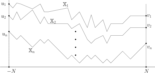
Figure 9. The family $\mathcal{P}^{\underline{u},\underline{v}}_{N,+}$

Let $\{V_{\lambda}\}_{\lambda>0}$ be a family of self-potentials $V_{\lambda}:\mathbb{N}_{0}\to\mathbb{R}_{+}$. Given a trajectory $\mathbb{X}\subset\mathbb{N}_{0}$ define

$$V_{\lambda}(\mathbb{X})=\sum_{i=-N}^{N}V_{\lambda}(X(i))\quad{\rm and}\quad{\mathsf{w}}_{\lambda}(\mathbb{X})={\rm e}^{-V_{\lambda}(\mathbb{X})}{\mathsf{p}}(\mathbb{X}).$$ (72)

The term $V_{\lambda}(\mathbb{X})$ represents a generalized (non-linear) area below the trajectory $\mathbb{X}$. It reduces to (a multiple of) the usual area if $V_{\lambda}(x)=\lambda x$. In general we make the following assumptions:

For any $\lambda>0$, the function $V_{\lambda}$ on $[0,\infty)$ is continuous, monotone increasing and satisfies

$$V_{\lambda}(0)=0\quad\text{ and }\quad\lim_{x\to\infty}V_{\lambda}(x)=\infty.$$ (73)

In particular, the relation

$$H_{\lambda}^{2}V_{\lambda}(H_{\lambda})=1$$ (74)

determines unambiguously the quantity $H_{\lambda}$. Furthermore, we make the assumptions that $\lim_{\lambda\downarrow 0}H_{\lambda}=\infty$ and that there exists a function $q\in\mathsf{C}^{2}(\mathbb{R}^{+})$ such that

$$\lim_{\lambda\downarrow 0}H_{\lambda}^{2}V_{\lambda}(rH_{\lambda})=q(r),$$ (75)

uniformly on compact subsets of $\mathbb{R}_{+}$. Note that $H_{\lambda}$, respectively $H_{\lambda}^{2}$, plays the role of the spatial, respectively temporal, scale in the invariance principle which is formulated below in Theorem 5.1.

A natural class of examples of family of potentials satisfying the above assumptions is given by $V_{\lambda}(x)=\lambda x^{\alpha}$ with $\alpha>0$. For the latter, $H_{\lambda}=\lambda^{-1/(2+\alpha)}$ and $q(r)=q_{0}(r)=r^{\alpha}$. In this way, the case of linear area tilts $\alpha=1$ corresponds to the familiar Airy rescaling $H_{\lambda}=\lambda^{-1/3}$.

Probability distributions

In the case of only one trajectory; $n=1$, given $u,v\in\mathbb{N}_{0}$ and $\lambda>0$, define the partition functions and probability distributions

$$Z^{u,v}_{N,+,\lambda}=\sum_{{\mathbb{X}}\in\mathcal{P}^{u,v}_{N,+}}{\mathsf{w}}_{\lambda}(\mathbb{X})\text{ and }\mathbb{P}^{u,v}_{N,+,\lambda}(\mathbb{X})=\frac{1}{Z^{uv}_{N,+,\lambda}}\,{\mathsf{w}}_{\lambda}(\mathbb{X})\mathbbm{1}_{\{\mathbb{X}\in\mathcal{P}^{u,v}_{N,+}\}}.$$ (76)

In the case of an $n$-tuple $\underline{\mathbb{X}}=(\mathbb{X}_{n},\ldots,\mathbb{X}_{1})$ of trajectories, we consider the product weights ${\mathsf{w}}_{\lambda}(\underline{\mathbb{X}})=\prod_{i=1}^{n}{\mathsf{w}}_{\lambda}(\mathbb{X}_{i})$ and define the probability distributions $\mathbb{P}^{\underline{u},\underline{v}}_{N,+,\lambda}$ on $\mathcal{P}^{\underline{u},\underline{v}}_{N,+}$ by

$$\mathbb{P}^{\underline{u},\underline{v}}_{N,+,\lambda}(\underline{\mathbb{X}})=\frac{1}{Z^{\underline{u},\underline{v}}_{N,+,\lambda}}\,{\mathsf{w}}_{\lambda}(\underline{\mathbb{X}})\mathbbm{1}_{\{\underline{\mathbb{X}}\in\mathcal{P}^{\underline{u},\underline{v}}_{N,+}\}}.$$ (77)

Rescaling and Invariance principle

The paths are rescaled as follows: For $t\in H_{\lambda}^{-2}\mathbb{Z}$, define

$$\underline{R}^{\lambda}(t)=\frac{1}{H_{\lambda}}\underline{\mathbb{X}}(H_{\lambda}^{2}t).$$ (78)

Then, extend $\underline{R}^{\lambda}$ to any $t\in\mathbb{R}$ by linear interpolation. In this way, given $T>0$ and $\underline{u},\underline{v}$, we can talk about the induced distribution $\mathbb{P}^{\underline{u},\underline{v};T}_{N,+,\lambda}$ on the space of continuous functions $\mathsf{C}\bigl{(}[-T,T],\mathbb{A}_{n}^{+}\bigr{)}$.

The result below was established in [48, 50] (under additional mild technical assumptions on $V_{\lambda}$):

Theorem 5.1.

For any $n=1,2,\dots$ fixed, the following happens: Let $\lambda_{N}$ be a sequence satisfying

$$\lim_{N\to\infty}\lambda_{N}=0\quad\text{ and }\quad\lim_{N\to\infty}\frac{N}{H_{\lambda_{N}}^{2}}=\infty.$$ (79)

Fix any $C\in(0,\infty)$ and any $T>0$. Then, the sequence of distributions $\mathbb{P}^{\underline{u},\underline{v};T}_{N,+,{\lambda_{N}}}$ converges weakly to the distribution $\mathbb{P}_{n}^{+;T}$ of the diffusion $\underline{R}(\cdot)$ in (100), uniformly in $u_{1},v_{1}\leq CH_{\lambda_{N}}$.

Notes on the proof

We refer to [48, 50] and to the earlier paper [42] for complete statements, further details and careful implementations. Here we shall try to indicate the main ideas.

STEP 1. Scaling: Consider the probability distribution (76) with polymer weights ${\mathsf{w}}_{\lambda}$ and try to guess what would be the typical height $H$ above the wall. There are two factors involved:

1. The price for the underlying random walk to stay below height $H$; for this one pays a constant each $H^{2}$ units of time.

2. The area tilt which exerts a price $V_{\lambda}(H)$ each time unit.

A balance between these two factors is achieved for $H$ satisfying $H^{2}V_{\lambda}(H)\sim\mathrm{const}$. Hence the choice (74).

STEP 2. Limiting Sturm–Liouville problem. Consider the partition functions $Z^{u,v}_{N,+,\lambda}$ in (76) with the polymer weights ${\mathsf{w}}_{\lambda}(\mathbb{X})$ specified in (72). Define

$$\mathsf{T}_{\lambda}f(x)=\sum_{y\in\mathbb{N}_{0}}p_{y-x}{\rm e}^{-V_{\lambda}(y)}f(y).$$ (80)

In this way, $Z^{u,v}_{N,+,\lambda}={\rm e}^{-V_{\lambda}(u)}(\mathsf{T}_{\lambda})^{2N}\delta_{v}(u)$. Let $f\in\mathsf{C}_{0}^{\infty}(0,\infty)$. Under the rescaling $x=H_{\lambda}r$; $r\in H_{\lambda}^{-1}\mathbb{N}_{0}\stackrel{{\scriptstyle\Delta}}{{=}}\mathbb{N}_{\lambda}$,

$$\begin{split}H_{\lambda}^{2}\left(\mathsf{T}_{\lambda}f(r)-f(r)\right)&=H_{\lambda}^{2}\sum_{s\in\mathbb{N}_{\lambda}}p_{H_{\lambda}(s-r)}{\rm e}^{-V_{\lambda}(H_{\lambda}s)}(f(s)-f(r))\\ &\hskip 85.35826pt+H_{\lambda}^{2}\Bigl{(}\sum_{s\in\mathbb{N}_{\lambda}}{\rm e}^{-V_{\lambda}(H_{\lambda}s)}-1\Bigr{)}f(r)\\ &\xrightarrow{\eqref{eq:HL-2},\eqref{eq:Assumption}}\frac{\sigma^{2}}{2}f^{\prime\prime}(r)-q(r)f(r),\end{split}$$ (81)

which suggests an application of Trotter–Kurtz theorem.

STEP 3. Use of the Karlin–McGregor formula in the case of $n$ ordered walks. The Slater determinants (99) naturally appear for the limiting ordered (continuous) Ferrari–Spohn diffusions via the Karlin–McGregor formula. However, an application for the discrete partition functions $Z^{\underline{u},\underline{v}}_{N,+,\lambda}$ in (77) requires some care. Indeed, the paths can jump over each other, and all the permutation terms in the general Karlin–McGregor formula [51] contribute. One shows, therefore, that as $\lambda\to 0$ the contribution of paths which jump over each other vanishes.

STEP 4. Mixing and compactness. As usual one needs to prove tightness. Furthermore, in order to show that the claim of Theorem 5.1 holds uniformly in the boundary conditions $\underline{u}$ and $\underline{v}$, one needs to prove mixing on $H_{\lambda}^{2}$-time scales. These are probabilistic estimates on random walks, which build upon initial considerations in [42]. In the case of $n$ ordered random walks, proving such mixing estimates is by far the most technically loaded part of [50], and it is based on recent strong approximation techniques developed in [26, 27, 32].

Appendix A Wulff shapes and Wulff plaquettes

Let $\varphi_{\beta}$ be a function on $\mathbb{R}^{d}$, which is convex and homogeneous of order one. We assume that $\varphi_{\beta}$ is positive on $\mathbb{R}^{d}\setminus\{0\}$ and that it respects the $\mathbb{Z}^{d}$-lattice symmetries. Depending on the context, the latter may represent either the surface tension $\varphi_{\beta}=\tau_{\beta}$ of low-temperature Ising models, as defined in (4), or the inverse correlation length $\varphi_{\beta}=\xi_{\beta}$ of low-temperature two-dimensional Ising polymers, as defined in (28).

Wulff shape.

By definition $\varphi_{\beta}$ is the support function of a symmetric compact convex set $\mathcal{W}_{\beta}$ with non empty interior,

$$\mathcal{W}_{\beta}=\bigcap_{\mathfrak{n}\in\mathbb{S}^{d-1}}\left\{x\in\mathbb{R}^{d}\,:\,x\cdot\mathfrak{n}\leq\varphi_{\beta}(\mathfrak{n})\right\}$$ (82)

In particular, this means that if ${\mathsf{n}}$ is a normal direction to the boundary $\partial\mathcal{W}_{\beta}$ at ${\mathsf{x}}\in\partial\mathcal{W}_{\beta}$, then $\varphi_{\beta}(\mathfrak{n})={\mathsf{x}}\cdot\mathfrak{n}$.

The set $\mathcal{W}_{\beta}$ is called the unnormalized Wulff shape associated to $\varphi_{\beta}$. It is convenient to consider the unit-volume rescaling $\mathsf{W}_{\beta}$ of $\mathcal{W}$ and the unit-radius rescaling $\mathsf{K}_{\beta}$ of $\mathcal{W}$:

$$\mathsf{W}_{\beta}=\frac{1}{\left|\mathcal{W}_{\beta}\right|^{1/d}}\mathcal{W}_{\beta}\quad{\rm and}\quad\mathsf{K}_{\beta}=\frac{1}{\varphi_{\beta}({\mathsf{e}_{1}})}\mathcal{W}.$$ (83)

Given a “sufficiently nice” (see [9] for more precision) subset $V\subset\mathbb{R}^{d}$, we define its surface energy

$$\varphi_{\beta}({V})\stackrel{{\scriptstyle\text{\tiny{\rm def}}}}{{=}}\int_{\partial V}\varphi_{\beta}(\mathfrak{n}_{s}){\rm d}s,$$

where $\mathfrak{n}_{s}$ denotes the normal to $\partial V$ at $s$. We consider the following isoperimetric-type variational problem:

(VP) Minimize $\varphi_{\beta}(\partial V)$ among all “sufficiently nice” sets $V$ of volume ${\mathsf{v}}$,

It can be shown [68] that, for any ${\mathsf{v}}>0$, the dilation ${{\mathsf{v}}}^{1/d}\mathsf{W}_{\beta}$ of $\mathsf{W}_{\beta}$ is the unique (up to translation) minimizer of (VP).

In two dimensions, equilibrium crystal shapes associated with surface tension are expected to have locally analytic and strictly convex boundaries. In the case of the nearest neighbor Ising model, there is an explicit formula for $\tau_{\beta}$. However, such a property should follow along the lines of the Ornstein–Zernike theory whenever phase separation lines admit an effective short-range random walk representation; see [16, 19] for such derivations in the context of percolation and Potts models.

In higher dimensions, low-temperature Ising Wulff shapes develop facets, at least in lattice directions [60]. Namely, for $\beta$ large, the (sub-differentials) sets $\partial\tau_{\beta}(\pm\mathsf{e}_{i})$ are proper $d-1$-dimensional pieces of $\partial\mathsf{W}_{\beta}$.

Two-dimensional constrained problems and Wulff plaquettes

Let us restrict attention to two dimensions. In view of the lattice symmetries, $\varphi_{\beta}(\mathsf{e})\stackrel{{\scriptstyle\Delta}}{{=}}\varphi_{\beta}(\pm\mathsf{e}_{i})$, where $\pm\mathsf{e}_{i}\;i=1,2$, are unit vectors in lattice coordinate directions, is well defined. That is, the rescaled shape $\mathsf{K}_{\beta}$ is inscribed into the square $[-1,1]^{2}$. Let us define the area $w_{\beta}$ of $\mathsf{K}_{\beta}$:

$$w_{\beta}=\left|\mathsf{K}_{\beta}\right|\in[2,4].$$ (84)

Recall that, given a rectifiable curve $\gamma$, its surface energy is defined by $\varphi_{\beta}(\gamma)=\int_{\gamma}\varphi_{\beta}(\mathfrak{n}_{s}){\rm d}s$. Consider the following constrained isoperimetric problem [65]:

(CVP) Minimize $\varphi_{\beta}(V)$ among all subsets $V\subset[-1,1]^{2}$ with rectifiable boundary $\partial V$ and area $\left|V\right|=\mathsf{b}\in(0,4]$.

The answer depends on the value of $\mathsf{b}$. It is natural to state it in terms of the unit-radius shape $\mathsf{K}_{\beta}$.

Since $\varphi_{\beta}(\cdot)$ is the support function of $\mathcal{W}_{\beta}$, the ratio $\frac{\varphi_{\beta}(\cdot)}{\varphi_{\beta}(\mathsf{e})}$ is the support function of $\mathsf{K}_{\beta}$. Hence,

$$w_{\beta}=\int_{\mathsf{K}_{\beta}}{\rm d}{\mathsf{x}}=\frac{1}{2}\int_{\mathsf{K}_{\beta}}\mathrm{div}({\mathsf{x}}){\rm d}{\mathsf{x}}=\frac{1}{2}\frac{\varphi_{\beta}(\partial\mathsf{K}_{\beta})}{\varphi_{\beta}(\mathsf{e})}\quad\Rightarrow\quad\varphi_{\beta}(\mathsf{K}_{\beta})=2\varphi_{\beta}(\mathsf{e})w_{\beta}.$$ (85)

In the above notation, the Wulff shape of area $\mathsf{b}$ is $\mathsf{K}_{\beta}^{\mathsf{b}}=\sqrt{\frac{\mathsf{b}}{w_{\beta}}}\mathsf{K}_{\beta}$ and, for $\mathsf{b}\in(0,w_{\beta}]$,

$$\varphi_{\beta}(\mathsf{b})\stackrel{{\scriptstyle\Delta}}{{=}}\min_{\begin{subarray}{c}V~{}:~{}\left|V\right|=\mathsf{b}\\ V\subseteq[-1,1]^{2}\end{subarray}}\varphi_{\beta}(V)=\varphi_{\beta}(\mathsf{K}_{\beta}^{\mathsf{b}})=2\varphi_{\beta}(\mathsf{e})\sqrt{{\mathsf{b}}{w_{\beta}}}.$$ (86)

Clearly, $\mathsf{K}_{\beta}^{\mathsf{b}}$ is the unique (again up to translations within $[-1,1]^{2}$) solution of (CVP) whenever $\mathsf{b}\in(0,w_{\beta}]$. Note that the radius $r_{\mathsf{b}}$ of $\mathsf{K}_{\beta}^{\mathsf{b}}$ satisfies

$$r_{\mathsf{b}}=\sqrt{\frac{\mathsf{b}}{w_{\beta}}}\quad{\rm and}\quad\frac{{\rm d}\varphi_{\beta}(\mathsf{K}_{\beta}^{\mathsf{b}})}{{\rm d}\mathsf{b}}=\frac{\varphi_{\beta}(\mathsf{e})}{r_{\mathsf{b}}}.$$ (87)

For $\mathsf{b}\in(w_{\beta},4]$, the shape $\mathsf{K}_{\beta}^{\mathsf{b}}$ does not fit into the square $[-1,1]^{2}$. In this case [65],

$$\varphi_{\beta}(\mathsf{b})\stackrel{{\scriptstyle\Delta}}{{=}}\min_{\begin{subarray}{c}V~{}:~{}\left|V\right|=\mathsf{b}\\ V\subseteq[-1,1]^{2}\end{subarray}}\varphi_{\beta}(V)=\varphi_{\beta}(\mathsf{P}^{\mathsf{b}}_{\beta})=\varphi_{\beta}(\mathsf{e})\cdot\Bigl{(}8-2\sqrt{(4-w_{\beta})(4-\mathsf{b})}\Bigr{)}.$$ (88)

Above, the Wulff plaquettes $\mathsf{P}^{\mathsf{b}}_{\beta}$ are constructed as follows: Place four Wulff shapes of radius

$$r_{\mathsf{b}}=\sqrt{\frac{4-\mathsf{b}}{4-w_{\beta}}}\leq 1$$ (89)

into the four corners of $[-1,1]^{2}$, in such a way that each of these shapes is tangent to the two corresponding sides of the square. Then take the convex envelope. Note that, by construction, $\partial\mathsf{P}^{\mathsf{b}}_{\beta}$ has four flat segments of length $2(1-r_{\mathsf{b}})$ on each of the four sides of $[-1,1]^{2}$. Also, note that in terms of $r_{\mathsf{b}}$. The area $\mathsf{b}$ and the surface energy $\varphi_{\beta}(\mathsf{P}_{\beta}^{\mathsf{b}})$ of the Wulff plaquette $\mathsf{P}_{\beta}^{\mathsf{b}}$ can be recorded as

$$\mathsf{b}=4-(4-w_{\beta})r_{\mathsf{b}}^{2},\ \varphi_{\beta}(\mathsf{P}_{\beta}^{\mathsf{b}})=\varphi_{\beta}(\mathsf{e})\left(8-2(4-w_{\beta})r_{\mathsf{b}}\right)\ {\rm and}\ \frac{{\rm d}\varphi_{\beta}(\mathsf{P}_{\beta}^{\mathsf{b}})}{{\rm d}\mathsf{b}}=\frac{\varphi_{\beta}(\mathsf{e})}{r_{\mathsf{b}}},$$ (90)

where the latter identity directly follows from (88) and (89).

Dual constrained variational problems

Let $\nu>0$ and consider:

(DCVP) Find  $\max_{\mathsf{a}\in[0,4]}\{\nu\mathsf{a}-\varphi_{\beta}(\mathsf{a})\}$.

By (86) and (88), the function $\varphi_{\beta}$ is concave on $[0,w_{\beta}]$ and convex on $[w_{\beta},4]$. Therefore, there exists a critical value $\nu_{\beta}\in(0,\infty)$ such that $\mathsf{a}=0$ is the unique solution to (DCVP) for $\nu\in[0,\nu_{\beta})$, while there is a unique solution $\mathsf{a}=\mathsf{a}(\beta,\nu)\in(w_{\beta},4)$ for every $\nu>\nu_{\beta}$. At $\nu=\nu_{\beta}$, there are two solutions: $\mathsf{a}=0$ and $\mathsf{a}=\mathsf{a}_{\beta}>w_{\beta}$. The critical pair $(\nu_{\beta},\mathsf{a}_{\beta})$ satisfies the following equation:

$$\varphi_{\beta}^{\prime}(\mathsf{a}_{\beta})=\varphi_{\beta}(\mathsf{e})\cdot\sqrt{\frac{4-w_{\beta}}{4-\mathsf{a}_{\beta}}}=\nu_{\beta}\text{ and }\nu_{\beta}\mathsf{a}_{\beta}=\varphi_{\beta}(\mathsf{e})\cdot\Bigl{(}8-2\sqrt{(4-w_{\beta})(4-\mathsf{a}_{\beta})}\Bigr{)}.$$ (91)

Geometrically, if one starts to rotate counter-clockwise a line passing through zero, then the latter will touch for the first time the graph of $\mathsf{a}\mapsto\varphi_{\beta}(\mathsf{a})$ at the angle $\nu_{\beta}$ and at the point $(\mathsf{a}_{\beta},\varphi_{\beta}(\mathsf{a}_{\beta}))$.

Note that, for $\nu>\nu_{\beta}$, the optimal shape is necessarily a Wulff plaquette and that there is a strict inclusion of optimal shapes that correspond to different $\nu^{\prime}>\nu>\nu_{\beta}$.

In order to get an explicit expression for the critical slope $\nu_{\beta}$, it is convenient to compare (91) with (90). Let $\rho_{\beta}$ be the critical radius. Then the first, and consequently the second, of (91) read as

$$\nu_{\beta}=\frac{\varphi_{\beta}(\mathsf{e})}{\rho_{\beta}}\quad{\rm and}\quad\frac{4-(4-w_{\beta})\rho_{\beta}^{2}}{\rho_{\beta}}=8-2(4-w_{\beta})\rho_{\beta}.$$ (92)

Solving the second of (92) (and taking into account that the solution we need should satisfy $\rho_{\beta}\leq 1$), we infer:

$$\rho_{\beta}=\frac{2}{2+\sqrt{w_{\beta}}}\ \Rightarrow\ \nu_{\beta}=\frac{\varphi_{\beta}(\mathsf{e})\left(2+\sqrt{w_{\beta}}\right)}{2}=\frac{4\varphi_{\beta}(\mathsf{e})+\varphi_{\beta}(\mathsf{W}_{\beta})}{4},$$ (93)

where we relied on (86) to identify the energy of the unit-volume Wulff shape as $\varphi_{\beta}(\mathsf{W}_{\beta})=2\varphi_{\beta}(\mathsf{e})\sqrt{w_{\beta}}$.

Appendix B Ferrari–Spohn diffusions

In this section, the notations $\|\cdot\|_{2}$ and $\langle\cdot,\cdot\rangle_{2}$ are reserved for the norm and scalar product in $\mathbb{L}_{2}(\mathbb{R}_{+})$.

Given $\sigma>0$ and a non-negative function $q\in\mathsf{C}^{2}(\mathbb{R}_{+})$ which satisfies $\lim_{r\to\infty}q(r)=\infty$, consider the following family of singular Sturm–Liouville operators on $\mathbb{R}_{+}$:

$$\mathsf{L}_{\sigma,q}=\frac{\sigma^{2}}{2}\frac{{\rm d}^{2}}{{\rm d}r^{2}}-q(r).$$ (94)

with boundary condition $\varphi(0)=0$. $\mathsf{L}_{\sigma,q}$ possesses a complete orthonormal family $\left\{\varphi_{i}\right\}$ of simple eigenfunctions in $\mathbb{L}_{2}(\mathbb{R}_{+})$ with eigenvalues

$$0>-\mathsf{e}_{0}>-\mathsf{e}_{1}>-\mathsf{e}_{2}>\dots;\ \lim\mathsf{e}_{j}=\infty.$$ (95)

The eigenfunctions $\varphi_{i}$ are smooth and $\varphi_{i}$ has exactly $i$ zeros in $(0,\infty)$, $i=0,1,\ldots$.

The Ferrari–Spohn diffusion, associated to $\sigma$ and $q$, is the diffusion on $(0,\infty)$ with generator

$$\mathsf{G}_{\sigma,q}\psi\stackrel{{\scriptstyle\Delta}}{{=}}\frac{1}{\varphi_{0}}(\mathsf{L}_{\sigma,q}+\mathsf{e}_{0})(\psi\varphi_{0})=\frac{\sigma^{2}}{2}\frac{{\rm d}^{2}\psi}{{\rm d}r^{2}}+\sigma^{2}\frac{\varphi_{0}^{\prime}}{\varphi_{0}}\frac{{\rm d}\psi}{{\rm d}r}=\frac{\sigma^{2}}{2\varphi_{0}^{2}}\frac{{\rm d}}{{\rm d}r}\Bigl{(}\varphi_{0}^{2}\frac{{\rm d}\psi}{{\rm d}r}\Bigr{)}.$$ (96)

This diffusion is ergodic and reversible with respect to the measure ${\rm d}\mu_{0}(r)=\varphi_{0}^{2}(r){\rm d}r$. We denote by $\mathsf{S}_{\sigma,q}^{t}$ the corresponding semigroup and by $\mathbb{P}_{\sigma,q}$ the associated path measure.

The most relevant case for the present paper is when the function $q$ is linear, $q(r)=cr$. In that case, since the Airy function $\sf Ai$ satisfies $\frac{{\rm d}^{2}}{{\rm d}r^{2}}{\sf Ai}(r)=r{\sf Ai}(r)$, one can easily check that

$$\varphi_{0}={\sf Ai}(\chi r-\omega_{1})\quad{\rm and}\quad e_{0}=\frac{c\omega_{1}}{\chi},$$ (97)

where $-\omega_{1}=-2.33811\ldots$ is the first zero of ${\sf Ai}$ and $\chi=\sqrt[3]{\frac{2c}{\sigma^{2}}}$.

Dyson Ferrari–Spohn diffusions

Let us fix $n\in\mathbb{N}$. Recall the notation

$$\mathbb{A}_{n}^{+}=\{\underline{r}\in\mathbb{R}^{n}\,:\,0\leq r_{n}\leq\dots\leq r_{1}\}.$$

Let $\underline{X}(t)=(\mathsf{X}_{n}(\cdot),\dots,\mathsf{X}_{1}(\cdot))$ be $n$ independent copies of Ferrari–Spohn diffusions starting at $\underline{r}\in\mathbb{A}_{n}^{+}$. Define the killing time

$$\tau=\min\{t\,:\,\underline{X}(t)\not\in\mathbb{A}_{n}^{+}\}.$$ (98)

In other words, $\tau$ is the minimum between the first collision time and the first time the bottom trajectory exits from the positive semi-axis. Dyson Ferrari–Spohn diffusion $\underline{R}(t)$ is $\underline{X}(\cdot)$ conditioned to survive forever, that is, conditioned on $\{\tau=\infty\}$. We refer to [50] for a precise construction. As is explained in the latter paper, a Dyson Ferrari–Spohn diffusion $\underline{R}(t)$ satisfies the following SDE: Let

$$\Delta(\underline{r})=\operatorname{det}\begin{bmatrix}\varphi_{1}(r_{1})&\varphi_{2}(r_{1})&\cdots&\varphi_{n}(r_{1})\\ \varphi_{1}(r_{2})&\varphi_{2}(r_{2})&\cdots&\varphi_{n}(r_{2})\\ \vdots&\vdots&\ddots&\vdots\\ \varphi_{1}(r_{n})&\varphi_{2}(r_{n})&\cdots&\varphi_{n}(r_{n})\end{bmatrix}.$$ (99)

be the Slater determinant of $\mathsf{L}_{\sigma,q}$. Alternatively, $\Delta(\underline{r})$ is the first Dirichlet eigenfunction of $\mathsf{L}_{n}+\dots+\mathsf{L}_{1}$ on $\mathbb{A}_{n}^{+}$, where $\mathsf{L}_{i}$ is a copy of $\mathsf{L}_{\sigma,q}$ acting on the $i$-th coordinate $r_{i}$. Then,

$${\rm d}\underline{R}(t)=\sigma{\rm d}\underline{B}(t)+\nabla\log(\Delta)(\underline{R}(t))\,{\rm d}t,$$ (100)

where $\underline{B}(t)$ is the standard $n$-dimensional Brownian motion. Note that the diffusion $\underline{R}(\cdot)$ on $\mathbb{A}_{n}^{+}$ is ergodic and reversible with respect to $\Delta^{2}(\underline{r})\,{\rm d}\underline{r}$. We use $\mathbb{P}_{n}^{+;T}$ to denote its (stationary) distribution on the space of continuous functions $\mathsf{C}\bigl{(}[-T,T],\mathbb{A}_{n}^{+}\bigr{)}$.

Appendix C Self-avoiding walks under area tilts

In this appendix, we shall sketch how Ferrari–Spohn diffusions appear as scaling limits of super-critical nearest-neighbor two-dimensional (vertex) self-avoiding walks (SAW-s) under area tilts. Being an instance of Ising polymers without cluster decorations super-critical SAW-s are viewed as simplified models of phase separation lines in 2D Ising models below critical temperature, and the discussion below is intended to reinforce Conjecture 3.2. A complete proof will hopefully appear elsewhere.

Let us fix $\beta>\log\mu_{c}$, where ${\mu_{c}}$ is the connectivity constant of $\mathbb{Z}^{2}$. In the sequel, we shall drop $\beta$ from all the notation. The reference weight of SAW trajectory $\gamma=\left(\gamma(0),\dots,\gamma(n)\right)$ is ${\rm e}^{-\beta n}={\rm e}^{-\beta\left|\gamma\right|}$. A path $\gamma$ is said to be a positive bridge, $\gamma\in\mathcal{B}^{+}$, if $\gamma\subset\mathbb{H}_{+}^{2}$ and if $\gamma(0)\cdot\mathsf{e}_{1}\leq\gamma(\ell)\cdot\mathsf{e}_{1}\leq\gamma(n)\cdot\mathsf{e}_{1}$. Given $x,y\in\mathbb{N}$, define

$$\mathcal{B}^{+}_{N}(x,y)=\left\{\gamma\in\mathcal{B}^{+}\,:\,\gamma(0)=(-N,x)\ {\rm and}\ \gamma(n)=(N,y)\right\}.$$ (101)

Note that $\left|\gamma\right|=n$ is not fixed in the above definition; we just talk about all the bridges from $(-N,x)$ to $(N,y)$. For any $\gamma\in\mathcal{B}^{+}$, the area $A(\gamma)$ is well defined. Given $\lambda>0$ (area tilt), consider the weights $w_{\lambda}$ and the probability distributions $\mathbb{P}_{N,+,\lambda}^{x,y}$:

$$w_{\lambda}(\gamma)={\rm e}^{-\beta\left|\gamma\right|-\lambda A(\gamma)}\quad{\rm and}\quad\mathbb{P}_{N,+,\lambda}^{x,y}(\gamma)=\frac{w_{\lambda}(\gamma)}{Z_{N,+,\lambda}^{x,y}}\mathbbm{1}_{\left\{\gamma\in\mathcal{B}^{+}_{N}(x,y)\right\}}.$$ (102)

We shall try to explore what happens when $\lambda\to 0$ and $N\to\infty$ in an appropriate way. The inverse correlation length $\xi_{\beta}$ is defined and positive for any $\beta>\log\mu_{c}$, and Ornstein–Zernike theory, as described in Subsection 4.3.1, applies [25, 43, 49]. Hence, for $\lambda$ sufficiently small and $N$ sufficiently large, we can restrict attention to $\gamma$ which admit an irreducible decomposition (51) with respect to some symmetric cone $\mathcal{Y}_{\mathsf{h}}$ along the horizontal axis, where $\mathsf{h}=\mathsf{h}_{\beta}=\nabla\xi_{\beta}(\mathsf{e}_{1})=\xi_{\beta}(\mathsf{e}_{1})\mathsf{e}_{1}$. If $\gamma$ admits (51), then we can think about linear interpolation $\hat{\gamma}$ through the vertices of (51). Notice that $\hat{\gamma}$ is already a well-defined function on $[-N,N]$. Let us rescale it as

$$x_{\lambda}(t)=\lambda^{1/3}\hat{\gamma}(\lambda^{-2/3}t).$$ (103)

Under $\mathbb{P}_{N,+,\lambda}^{x,y}$, the rescaled path $x_{\lambda}(\cdot)$ is viewed as a random continuous function on $[-N\lambda^{2/3},N\lambda^{2/3}]$. Here is the SAW counterpart of Conjecture 3.2:

Theorem C.1.

Consider $\lambda=\lambda_{N}$ which satisfies $\lim\lambda_{N}=0$ and $\lim N\lambda_{N}^{2/3}=\infty$. Consider a sequence $\left\{x_{N},y_{N}\right\}$ of boundary conditions, such that $x_{N},y_{N}\leq C\lambda_{N}^{-1/3}$.

Then the distribution of $x_{\lambda_{N}}(\cdot)$ under $\mathbb{P}_{N,+,\lambda}^{x_{N},y_{N}}$ is weakly convergent to the distribution of FS diffusion with parameters $\sigma^{2}=\chi_{\beta}$ and $q(r)=r$, where $\chi_{\beta}$ is the curvature of $\partial\mathcal{W}_{\beta}$ at $\mathsf{h}_{\beta}$.

Below we indicate main steps of the proof.

STEP 1. Identification of $\chi_{\beta}$ in terms of the probability distribution $\mathbb{P}_{\beta}^{\mathsf{h}}$ (compare with (46)) on the set of irreducible animals/paths $\mathsf{D}\stackrel{{\scriptstyle\Delta}}{{=}}\mathsf{D}_{\mathsf{h}}$:

$$\mathbb{P}_{\beta}^{\mathsf{h}}(\mathfrak{a})={\rm e}^{\mathsf{h}\cdot\mathsf{X}(\mathfrak{a})-\beta\left|\gamma\right|}.$$ (104)

By (49) the boundary $\partial\mathcal{W}_{\beta}$ is parametrized around $\mathsf{h}$ as $t\to\phi(t)$ with

$$\mathbb{E}_{\beta}^{\mathsf{h}}\left({\rm e}^{(-\phi(t),t)\cdot\mathsf{X}}\right)\equiv 1.$$ (105)

Writing $\mathsf{X}=(\mathsf{T},\mathsf{Y})$ one, using symmetry of $\mathsf{Y}$ under $\mathbb{P}_{\beta}^{\mathsf{h}}$ and second order expansion, recovers $\chi_{\beta}$ as

$$\chi_{\beta}=\frac{\mathbb{E}_{\beta}^{\mathsf{h}}(\mathsf{Y}^{2})}{\mathbb{E}_{\beta}^{\mathsf{h}}(\mathsf{T})}.$$ (106)

STEP 2. Reduction to effective Markov chains. Instead of $\mathcal{B}_{N}^{+}$, consider the concatenations of, say, $m$ irreducible pieces. It happens to be convenient to record such concatenation as

$$\left\{\mathfrak{a}_{1},x_{1}\right\}\circ\left\{\mathfrak{a}_{2},x_{2}\right\}\circ\cdots\circ\left\{\mathfrak{a}_{m},x_{m}\right\}.$$ (107)

We understand a pair $\{\mathfrak{a},x\}$ as an animal $\mathfrak{a}$ being attached to a point at height $x\in\mathbb{N}$ from the left, and we write $\{\mathfrak{a},x\}\in\mathcal{S}_{+}$ if the resulting structure is inside $\mathbb{H}_{+}^{2}$. Let us record the area

$$A\left(\left\{\mathfrak{a},x\right\}\right)=\left(x-\mathsf{Y}(\mathfrak{a})\right)\mathsf{T}(\mathsf{a})+\Delta(\mathfrak{a}),$$ (108)

where it should be understood that the above relation defines $\Delta(\mathfrak{a})$.

A pair $\{\mathfrak{a},x\}\in\mathcal{S}_{+}$ and its area $A(\{\mathfrak{a},x\})$

Finally define a sub-Markov kernel $\mathsf{Q}_{\lambda}$ on $\mathcal{S}_{+}$:

$$Q_{\lambda}\left(\left\{\mathfrak{a},u\right\},\left\{\mathfrak{b},v\right\}\right)=\mathbbm{1}_{\left\{u=v-\mathsf{Y}(\mathfrak{b})\right\}}\mathbb{P}_{\beta}^{\mathsf{h}}(\mathfrak{b}){\rm e}^{-\lambda A\left(\left\{\mathfrak{b},v\right\}\right)}.$$ (109)

In this way, we can record various partition functions in terms of powers of $Q_{\lambda}$. For instance, the partition function of all $m$-irreducible step trajectories from height $x$ to height $y$ reads as:

$$\sum_{\begin{subarray}{c}\left\{\mathfrak{a},u\right\}\in\mathcal{S}_{+}\\ u-\mathsf{Y}(\mathfrak{a})=x\end{subarray}}\sum_{\mathfrak{b}:\left\{\mathfrak{b},y\right\}\in\mathcal{S}_{+}}Q_{\lambda}^{m}\left(\left\{\mathfrak{a},u\right\},\left\{\mathfrak{b},y\right\}\right)$$ (110)

Path of irreducible steps from $x$ to $y$.

STEP 3. Rescaling and application of Trotter–Kurtz theorem. As before, define $\mathbb{N}_{\lambda}=\lambda^{1/3}\mathbb{N}$. For $r,s\in\mathbb{N}$, consider the rescaled sub-Markov kernel

$$\hat{Q}_{\lambda}(\{\mathfrak{a},r\},\{\mathfrak{b},s\})=Q_{\lambda}(\{\mathfrak{a},r\lambda^{-1/3}\},\{\mathfrak{b},s\lambda^{-1/3}\}).$$ (111)

Let $f\in\mathsf{C}_{0}^{\infty}\left(0,\infty\right)$. Given $r\in\mathbb{N}_{\lambda}$ and $\mathfrak{a}$ such that $\left\{\mathfrak{a},\lambda^{-1/3}r\right\}\in\mathcal{S}_{+}$, notice that

$$\frac{1}{\lambda^{2/3}} \Bigl{(}\sum_{\left\{\mathfrak{b},s\right\}}\hat{Q}_{\lambda}\left(\left\{\mathfrak{a},r\right\},\left\{\mathfrak{b},s\right\}\right)f(s)-f(r)\Bigr{)}$$ (112)

$$\stackrel{{\scriptstyle\eqref{eq:Q-lambda}}}{{=}}\frac{1}{\lambda^{2/3}}\Bigl{(}\sum_{\mathfrak{b}\in\mathsf{D}}\mathbbm{1}_{\left\{\lambda^{-1/3}r+\mathsf{b}\subset\mathbb{H}_{+}^{2}\right\}}\mathbb{P}_{\beta}^{h}(\mathfrak{b}){\rm e}^{-\lambda(\lambda^{-1/3}r\mathsf{T}(\mathfrak{b})+\Delta(\mathfrak{b}))}f(r+\lambda^{1/3}\mathsf{Y}(\mathfrak{b}))-f(r)\Bigr{)}$$ (113)

$$=\frac{\mathbb{E}_{\beta}^{\mathsf{h}}(\mathsf{Y}^{2})}{2}f^{\prime\prime}(r)-\mathbb{E}_{\beta}^{\mathsf{h}}(\mathsf{T})rf(r)+{\mathrm{o}}\left(1\right)\stackrel{{\scriptstyle\eqref{eq:chi-b-var}}}{{=}}\mathbb{E}_{\beta}^{\mathsf{h}}(\mathsf{T})\bigl{(}\frac{\chi_{\beta}}{2}f^{\prime\prime}(r)-rf(r)+{\mathrm{o}}\left(1\right)\bigr{)}$$ (114)

$$\stackrel{{\scriptstyle\Delta}}{{=}}\mathbb{E}_{\beta}^{\mathsf{h}}(\mathsf{T})\mathsf{L}_{\beta}f+{\mathrm{o}}\left(1\right).$$ (115)

This, when relying on Theorem I.6.5 in [33], means that, for any $t>0$, any $g,f\in\mathsf{C}_{0}^{\infty}(0,\infty)$ and any $\mathfrak{a}\in\mathsf{D}$,

$$\lim_{\lambda\to 0}\lambda^{1/3}\sum_{r,s\in\mathbb{N}_{\lambda}}\sum_{\mathfrak{b}\in\mathsf{D}}g(r)\hat{Q}_{\lambda}^{\lfloor t\lambda^{-2/3}/\mathbb{E}_{\beta}^{\mathsf{h}}(\mathsf{T})\rfloor}\left(\left\{\mathfrak{a},r\right\},\left\{\mathfrak{b},s\right\}\right)f(s)=\int_{0}^{\infty}f(r){\rm e}^{t\mathsf{L}_{\beta}}g(r){\rm d}r.$$ (116)

STEP 4. Mixing and tightness for the rescaling (103) of $\hat{\gamma}$ follows by arguments similar to those employed in the case of the usual random walk in [48]. Mixing is needed for coupling distributions with fixed horizontal projections as in (102) with distributions which correspond to a fixed number of irreducible steps, as generated by the sub-Markov kernel (109), as well as for coupling distributions with different numbers of irreducible steps and with the limiting ergodic Markov chain on $\mathsf{S}_{+}$, which is defined for any $\lambda>0$. Once mixing is established, (116) implies convergence of the finite-dimensional distributions of $x_{\lambda}$ to the finite-dimensional distributions of the FS $(\chi_{\beta},r)$-diffusion, which is upgraded to a full invariance principle by tightness.

References

- [1] D. B. Abraham. Solvable model with a roughening transition for a planar Ising ferromagnet. Phys. Rev. Lett., 44:1165–1168, 1980.
- [2] K. Alexander, J. T. Chayes, and L. Chayes. The Wulff construction and asymptotics of the finite cluster distribution for two-dimensional Bernoulli percolation. Comm. Math. Phys., 131(1):1–50, 1990.
- [3] K. S. Alexander. Cube-root boundary fluctuations for droplets in random cluster models. Comm. Math. Phys., 224(3):733–781, 2001.
- [4] K. S. Alexander, F. Dunlop, and S. Miracle-Solé. Layering in the Ising model. J. Stat. Phys., 141(2):217–241, 2010.
- [5] K. S. Alexander, F. Dunlop, and S. Miracle-Solé. Layering and wetting transitions for an SOS interface. J. Stat. Phys., 142(3):524–576, 2011.
- [6] A. G. Basuev. A series of phase transitions of the first kind for the Ising model in a half space. Dokl. Akad. Nauk SSSR, 299(4):854–857, 1988.
- [7] A. G. Basuev. The Ising model in a half-space: a series of phase transitions in small magnetic fields. Teoret. Mat. Fiz., 153(2):220–261, 2007.
- [8] M. Biskup, L. Chayes, and R. Kotecký. Critical region for droplet formation in the two-dimensional Ising model. Comm. Math. Phys., 242(1-2):137–183, 2003.
- [9] T. Bodineau, D. Ioffe, and Y. Velenik. Rigorous probabilistic analysis of equilibrium crystal shapes. J. Math. Phys., 41(3):1033–1098, 2000. Probabilistic techniques in equilibrium and nonequilibrium statistical physics.
- [10] T. Bodineau, D. Ioffe, and Y. Velenik. Winterbottom construction for finite range ferromagnetic models: an -approach. J. Statist. Phys., 105(1-2):93–131, 2001.
- [11] T. Bodineau, R. H. Schonmann, and S. Shlosman. 3D crystal: how flat its flat facets are? Comm. Math. Phys., 255(3):747–766, 2005.
- [12] J. Bricmont, A. El Mellouki, and J. Fröhlich. Random surfaces in statistical mechanics: roughening, rounding, wetting,… J. Statist. Phys., 42(5-6):743–798, 1986.
- [13] J. Bricmont and J. L. Lebowitz. Wetting in Potts and Blume-Capel models. J. Statist. Phys., 46(5-6):1015–1029, 1987.
- [14] J. Bricmont, J. L. Lebowitz, and C. E. Pfister. On the surface tension of lattice systems. In Third International Conference on Collective Phenomena (Moscow, 1978), volume 337 of Ann. New York Acad. Sci., pages 214–223. New York Acad. Sci., New York, 1980.
- [15] J. Bricmont and J. Slawny. Phase transitions in systems with a finite number of dominant ground states. J. Statist. Phys., 54(1-2):89–161, 1989.
- [16] M. Campanino and D. Ioffe. Ornstein-Zernike theory for the Bernoulli bond percolation on . Ann. Probab., 30(2):652–682, 2002.
- [17] M. Campanino, D. Ioffe, and O. Louidor. Finite connections for supercritical Bernoulli bond percolation in 2D. Markov Process. Related Fields, 16(2):225–266, 2010.
- [18] M. Campanino, D. Ioffe, and Y. Velenik. Ornstein-Zernike theory for finite range Ising models above . Probab. Theory Related Fields, 125(3):305–349, 2003.
- [19] M. Campanino, D. Ioffe, and Y. Velenik. Fluctuation theory of connectivities for subcritical random cluster models. Ann. Probab., 36(4):1287–1321, 2008.
- [20] E. Caputo, P.and Lubetzky, F. Martinelli, A. Sly, and F. L. Toninelli. Scaling limit and cube-root fluctuations in SOS surfaces above a wall. J. Eur. Math. Soc. (JEMS), 18(5):931–995, 2016.
- [21] P. Caputo, E. Lubetzky, F. Martinelli, A. Sly, and F. L. Toninelli. Dynamics of -dimensional SOS surfaces above a wall: slow mixing induced by entropic repulsion. Ann. Probab., 42(4):1516–1589, 2014.
- [22] P. Caputo, F. Martinelli, and F. L. Toninelli. On the probability of staying above a wall for the -dimensional SOS model at low temperature. Probab. Theory Related Fields, 163, 2015.
- [23] F. Cesi and F. Martinelli. On the layering transition of an SOS surface interacting with a wall. I. Equilibrium results. J. Statist. Phys., 82(3-4):823–913, 1996.
- [24] J. T. Chalker. The pinning of an interface by a planar defect. J. Phys. A, 15(9):L481–L485, 1982.
- [25] J. T. Chayes and L. Chayes. Ornstein-Zernike behavior for self-avoiding walks at all noncritical temperatures. Comm. Math. Phys., 105(2):221–238, 1986.
- [26] D. Denisov and V. Wachtel. Conditional limit theorems for ordered random walks. Electron. J. Probab., 15:no. 11, 292–322, 2010.
- [27] D. Denisov and V. Wachtel. Random walks in cones. Ann. Probab., 43(3):992–1044, 2015.
- [28] J.-D. Deuschel, G. Giacomin, and L. Zambotti. Scaling limits of equilibrium wetting models in -dimension. Probab. Theory Related Fields, 132(4):471–500, 2005.
- [29] E. I. Dinaburg and A. E. Mazel. Layering transition in SOS model with external magnetic field. J. Statist. Phys., 74(3-4):533–563, 1994.
- [30] R. Dobrushin, R. Kotecký, and S. Shlosman. Wulff construction, volume 104 of Translations of Mathematical Monographs. American Mathematical Society, Providence, RI, 1992. A global shape from local interaction, Translated from the Russian by the authors.
- [31] R. L. Dobrushin. Gibbs states describing a coexistence of phases for the three-dimensional Ising model. Th.Prob. and its Appl., 17(3):582–600, 1972.
- [32] J. Duraj and V. Wachtel. Invariance principles for random walks in cones. Preprint, arXiv:1508.07966, 2015.
- [33] S. N. Ethier and T. G. Kurtz. Markov processes. Wiley Series in Probability and Mathematical Statistics: Probability and Mathematical Statistics. John Wiley & Sons Inc., New York, 1986. Characterization and convergence.
- [34] P. L. Ferrari and H. Spohn. Constrained Brownian motion: fluctuations away from circular and parabolic barriers. Ann. Probab., 33(4):1302–1325, 2005.
- [35] S. Friedli, D. Ioffe, and Y. Velenik. Subcritical percolation with a line of defects. Ann. Probab., 41(3B):2013–2046, 2013.
- [36] J. Fröhlich and C.-E. Pfister. Semi-infinite Ising model. I. Thermodynamic functions and phase diagram in absence of magnetic field. Comm. Math. Phys., 109(3):493–523, 1987.
- [37] J. Fröhlich and C.-E. Pfister. Semi-infinite Ising model. II. The wetting and layering transitions. Comm. Math. Phys., 112(1):51–74, 1987.
- [38] J. Fröhlich and T. Spencer. The Kosterlitz-Thouless transition in two-dimensional abelian spin systems and the Coulomb gas. Comm. Math. Phys., 81(4):527–602, 1981.
- [39] L. Greenberg and D. Ioffe. On an invariance principle for phase separation lines. Ann. Inst. H. Poincaré Probab. Statist., 41(5):871–885, 2005.
- [40] P. Holický and M. Zahradník. On entropic repulsion in low temperature Ising models. In Cellular automata and cooperative systems (Les Houches, 1992), volume 396 of NATO Adv. Sci. Inst. Ser. C Math. Phys. Sci., pages 275–287. Kluwer Acad. Publ., Dordrecht, 1993.
- [41] O. Hryniv and R. Kotecký. Surface tension and the Ornstein-Zernike behaviour for the 2D Blume-Capel model. J. Statist. Phys., 106(3-4):431–476, 2002.
- [42] O. Hryniv and Y. Velenik. Universality of critical behaviour in a class of recurrent random walks. Probab. Theory Related Fields, 130(2):222–258, 2004.
- [43] D. Ioffe. Ornstein-Zernike behaviour and analyticity of shapes for self-avoiding walks on . Markov Process. Related Fields, 4(3):323–350, 1998.
- [44] D. Ioffe and R. H. Schonmann. Dobrushin-Kotecký-Shlosman theorem up to the critical temperature. Comm. Math. Phys., 199(1):117–167, 1998.
- [45] D. Ioffe and S. Shlosman. Ising model fog drip: the first two droplets. In In and out of equilibrium. 2, volume 60 of Progr. Probab., pages 365–381. Birkhäuser, Basel, 2008.
- [46] D. Ioffe and S. Shlosman. Formation of facets for an effective model of crystal growth. arXiv:1704.06760, 2017.
- [47] D. Ioffe, S. Shlosman, and F. L. Toninelli. Interaction versus entropic repulsion for low temperature Ising polymers. J. Stat. Phys., 158(5):1007–1050, 2015.
- [48] D. Ioffe, S. Shlosman, and Y. Velenik. An invariance principle to Ferrari-Spohn diffusions. Comm. Math. Phys., 336(2):905–932, 2015.
- [49] D. Ioffe and Y. Velenik. Ballistic phase of self-interacting random walks. In P. Mörters, R. Moser, M. Penrose, H. Schwetlick, and J. Zimmer, editors, Analysis and Stochastics of Growth Processes and Interface Models, pages 55–79. Oxford University Press, 2008.
- [50] D. Ioffe, Y. Velenik, and V. Wachtel. Dyson Ferrari–Spohn diffusions and ordered walks under area tilts. Probab. Theory Relat. Fields, 2017. https://doi.org/10.1007/s00440-016-0751-z.
- [51] S. Karlin and J. McGregor. Coincidence probabilities. Pacific J. Math., 9:1141–1164, 1959.
- [52] H. Lacoin. Wetting and layering for Solid-on-Solid I: Identification of the wetting point and critical behavior. arXiv:1703.06162, 2017.
- [53] H. Lacoin. Wetting and layering for Solid-on-Solid II: Layering transitions, Gibbs states, and regularity of the free energy. arXiv:1712.03736, 2017.
- [54] J. L. Lebowitz and C. Maes. The effect of an external field on an interface, entropic repulsion. J. Statist. Phys., 46(1-2):39–49, 1987.
- [55] J. L. Lebowitz and A. E. Mazel. A remark on the low-temperature behavior of the SOS interface in half-space. J. Statist. Phys., 84(3-4):379–397, 1996.
- [56] J. L. Lebowitz and C. E. Pfister. Surface tension and phase coexistence. Phys. Rev. Lett., 46(15):1031–1033, 1981.
- [57] E. Lubetzky, F. Martinelli, and A. Sly. Harmonic pinnacles in the Discrete Gaussian model. arXiv:1405.5241, 2014.
- [58] A. Messager, S. Miracle-Solé, and J. Ruiz. Convexity properties of the surface tension and equilibrium crystals. J. Statist. Phys., 67(3-4):449–470, 1992.
- [59] S. Miracle-Sole. Surface tension, step free energy, and facets in the equilibrium crystal. Journal of Statistical Physics, 79(1):183–214, 1995.
- [60] S. Miracle-Sole. Facet shapes in a Wulff crystal. In Mathematical results in statistical mechanics (Marseilles, 1998), pages 83–101. World Sci. Publ., River Edge, NJ, 1999.
- [61] C.-E. Pfister. Large deviations and phase separation in the two-dimensional Ising model. Helv. Phys. Acta, 64(7):953–1054, 1991.
- [62] C.-E. Pfister and Y. Velenik. Mathematical theory of the wetting phenomenon in the 2D Ising model. Helv. Phys. Acta, 69(5-6):949–973, 1996.
- [63] C.-E. Pfister and Y. Velenik. Large deviations and continuum limit in the D Ising model. Probab. Theory Related Fields, 109(4):435–506, 1997.
- [64] C.-E. Pfister and Y. Velenik. Interface, surface tension and reentrant pinning transition in the D Ising model. Comm. Math. Phys., 204(2):269–312, 1999.
- [65] R. H. Schonmann and S. B. Shlosman. Constrained variational problem with applications to the Ising model. J. Statist. Phys., 83(5-6):867–905, 1996.
- [66] W. Selke and J. Yeomans. Interface properties of the two-dimensional Blume-Emery-Griffiths model. Journal of Physics A: Mathematical and General, 16(12):2789, 1983.
- [67] A. Soshnikov. Determinantal random point fields. Uspekhi Mat. Nauk, 55(5(335)):107–160, 2000.
- [68] J. E. Taylor. Crystalline variational problems. Bull. Amer. Math. Soc., 84(4):568–588, 1978.
- [69] Y. Velenik. Entropic repulsion of an interface in an external field. Probab. Theory Related Fields, 129(1):83–112, 2004.