]Also at Andronikashvili Institute of Physics, 0177 Tbilisi, Georgia

Spin-Orbit Dimers and Non-Collinear Phases in $d^{1}$ Cubic Double Perovskites

Abstract

We formulate and study a spin-orbital model for a family of cubic double perovskites with $d^{1}$ ions occupying a frustrated fcc sublattice. A variational approach and a complimentary analytical analysis reveal a rich variety of phases emerging from the interplay of Hund’s and spin-orbit couplings (SOC). The phase digram includes non-collinear ordered states, with or without net moment, and, remarkably, a large window of a non-magnetic disordered spin-orbit dimer phase. The present theory uncovers the physical origin of the unusual amorphous valence bond state experimentally suggested for Ba₂BMoO₆ (B=Y,Lu), and predicts possible ordered patterns in Ba₂BOsO₆ (B=Na,Li) compounds.

Conventionally, frustration, low dimensionality and low spin are the key attributes of emerging novel quantum ground states. In the quest to realize a quantum spin liquid, a state of spins possessing massive quantum entanglement and lacking magnetic order, researchers have extensively studied Mott insulators with antiferromagnetic (AF) interactions on geometrically frustrated triangular, kagome, hyper-kagome and pyrochlore lattices Balents (2010); Savary and Balents (2016). Another route to frustration in Mott insulators with unquenched angular momentum is provided by orbital degrees of freedom. The directional character of degenerate $d$-orbitals may frustrate the magnetic interactions even on bipartite lattices, and lead to a plethora of emergent phases with unusual spin patterns  Kugel and Khomskii (1982); Khaliullin (2005) or without long-range spin/orbital order Pen et al. (1997); Khaliullin and Maekawa (2000); Vernay et al. (2004); Di Matteo et al. (2004, 2005); Jackeli and Khomskii (2008).

In $4d$ and $5d$ transition metal compounds, the enhanced SOC, compared to $3d$ systems, fully or partly lifts the local degeneracy of a $d$-shell. When degeneracy is fully lifted, e.g. in case of a single hole in a $t_{2g}$-shell, the anisotropic orbital interactions as well as related frustration are transferred to pseudo-spin one-half Kramers doublets of $d^{5}$ ions Khaliullin (2005); Chen and Balents (2008); Jackeli and Khaliullin (2009). However, in case of only partially lifting the degeneracy, the directional character of the electron density of the degenerate states is preserved, resulting in an effective reduction of magnetic sublattice dimensionality and strongly amplifying the effects of geometrical frustration. The Mott insulating $d^{1}$ double perovskites with undistorted cubic structure, such as spin-1/2 Ba₂BMoO₆ (B=Y,Lu) and Ba₂BOsO₆ (B=Na,Li), in which the only magnetically active ions, Mo⁵⁺ or Os⁷⁺, reside on a weakly frustrated fcc sublattice well exemplify this physical scenario Chen et al. (2010).

The osmium compounds Ba₂NaOsO₆ and Ba₂LiOsO₆ order magnetically Stitzer et al. (2002); Erickson et al. (2007); Steele et al. (2011). Small effective local moments $\sim\!0.7\;\mu_{\rm B}$, compared to spin only value 1.7 $\mu_{\rm B}$, have been extracted from high temperature susceptibilities in both materials Stitzer et al. (2002). The strong reduction of local moments is a direct manifestation of unquenched orbital momentum and strong SOC in the $5d$-shell of Os⁷⁺ ion Lee and Pickett (2007); Gangopadhyay and Pickett (2015, 2016). In Ba₂NaOsO₆, anomalously small net ordered moment $\sim\!0.2\mu_{\rm B}$ has additionally been detected Erickson et al. (2007); Steele et al. (2011). Recent NMR measurements indicate a canted AF order in the Na compound Lu et al. (2017).

The reported experimental data on Ba₂YMoO₆ are even more puzzling: this compound does not show any structural or magnetic transition down to $50$ mK Aharen et al. (2010); de Vries et al. (2010, 2013). The total high temperature entropy extracted from electronic heat capacity was reported to be close to $R\ln 4$ de Vries et al. (2010), indicating the presence of an extra two-fold orbital degeneracy in addition to the spin, and allowing for the emergence of multi-orbital physics. Based on magnetic susceptibility and muon spin rotation data, a valence bond glass state, an amorphous arrangement of spin singlets, has been proposed for Ba₂YMoO₆ de Vries et al. (2010) which remains quite stable against isovalent substitutions of Ba²⁺ with Sr²⁺ Mclaughlin et al. (2010). The magnetic susceptibility of a very similar compound Ba₂LuMoO₆ also did not exhibit any magnetic transition down to 2 K Coomer and Cussen (2013). Theoretically, various exotic phases, including multipolar order Chen et al. (2010) and chiral spin-orbital liquid Natori et al. (2016), have been put forward as possible candidates.

In this letter, we introduce and study a spin-orbital model and show that a dimer-singlet phase, composed of random arrangement of spin-orbit dimers, without any type of long-range order is a natural ground state of the model. The physical properties of this disordered phase are consistent with all available experimental findings on molybdenum double perovskites. In addition, the minimal model supports complex non-collinear, coplanar, ordered patterns. We argue that such four-sublattice ordered states are realised in osmium compounds.

Local electronic structure.– The single $d$-electron of a Mo⁵⁺ or Os⁷⁺ ion in a cubic environment occupies $t_{2g}\text{-manifold}$ of degenerate $xy$, $xz$, $yz$ orbitals. It carries an effective angular momentum $l=1$ with $|l^{z}\!\!=\!\!0\rangle\equiv\!\!|xy\rangle$, $|l^{z}\!\!=\!\!\pm 1\rangle\equiv\!\!-\frac{1}{\sqrt{2}}(i|xz\rangle\pm|yz\rangle)$ Abragam and Bleaney (1970). The six-fold degeneracy of the local Hilbert space is lifted by the local SOC $H_{\rm so}=-\lambda{\vec{l}}\cdot{\vec{S}}$ stabilizing $j=l+S=\frac{3}{2}$ quartet and pushing $j=\frac{1}{2}$ Kramers doublet to a higher energy. Here, ${\vec{S}}$ is an electron spin operator and $\lambda$ denotes the SOC. The states $j^{z}=\pm\frac{1}{2}$ of $j=\frac{3}{2}$ manifold have predominantly $xy$ character, while $j^{z}=\pm\frac{3}{2}$ components are given by superposition of $xz$ and $yz$ orbitals only [see Fig. 1(a)]. When SOC is much smaller (larger) than the exchange interactions between neigbhoring ions, it is more convenient to use the $t_{2g}$ ($j=\frac{3}{2}$) basis. The following analysis covers both limits.

Spin-orbital Hamiltonian.– In the double perovskite structure, each nearest-neighbor bond of the fcc sublattice of magnetic ions belongs to one of the crystallographic planes $xy$, $xz$, or $yz$ as shown in Fig. 1(b). We label these bonds as well as the $t_{2g}$-orbitals with a cubic axis $\gamma(=a,b,c)$ normal to their planes, e.g. $xy$ becomes $c$. The hopping between neighboring $t_{2g}$-orbitals takes place through intermediate oxygens’ $p$-orbitals, or direct hybridization. Along a $\gamma$-type bond the dominant overlap, with amplitude $t$, is between $\gamma$-orbitals Chen et al. (2010); Str . The low-energy spin-orbital model is obtained via standard second order perturbation theory in $t/U$ ($U$ being the local Coulomb repulsion) tU , and reads as follows:

$${\cal H} = \sum_{\langle ij\rangle_{\gamma}}{\Bigr{[}}-J_{1}{\bigr{(}}\vec{S}_{i}\cdot\vec{S}_{j}+\frac{3}{4}{\bigl{)}}+J_{2}{\bigr{(}}\vec{S}_{i}\cdot\vec{S}_{j}-\frac{1}{4}{\bigl{)}{\Bigl{]}}}P_{ij}^{(\gamma)}$$ (1)

$$+ J_{3}\sum_{\langle ij\rangle_{\gamma}}{\bigr{(}}\vec{S}_{i}\cdot\vec{S}_{j}-\frac{1}{4}{\bigl{)}}\bar{P}_{ij}^{(\gamma)}-\lambda\sum_{i}{\vec{l}}\cdot{\vec{S}}~{}.$$

${\langle ij\rangle_{\gamma}}$ denotes a $\gamma$-type bond, $J_{1(2)}=\frac{1}{4}Jr_{1(2)}$, $J_{3}=\frac{1}{3}J(2r_{2}+r_{3})$, $J=4t^{2}/U$, the set of $r_{n}$ describing the multiplet structure of excited states are functions of $\eta=J_{H}/U\ll 1$ rva , and $J_{H}$ is the Hund’s coupling.

The isotropic spin exchange couplings depend on the orbital occupancy of the corresponding bonds Kugel and Khomskii (1982); SM , and are described by the first three terms of Eq. (1), with the orbital projectors $P_{ij}^{(\gamma)}=n_{i}^{(\gamma)}(1-n_{j}^{(\gamma)})+(1-n_{i}^{(\gamma)})n_{j}^{(\gamma)}$ and $\bar{P}_{ij}^{(\gamma)}=n_{i}^{(\gamma)}n_{j}^{(\gamma)}$, where $n_{i}^{(\gamma)}$ is the occupation number of a $\gamma$-orbital. The spin isotropy is broken by the SOC in Eq. (1), allowing symmetric anisotropic exchange between $j=\frac{3}{2}$ quartets. In cubic double perovskites, the antisymmetric Dzyaloshinsky-Moriya exchange is forbidden by the bond inversion symmetry.

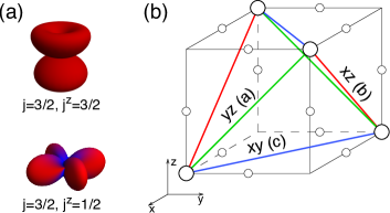
Figure 1: (a) Density profile of $j=3/2$ quartet. The states $j^{z}=\pm\frac{1}{2}$ (bottom) have dominant $xy$-orbital character, while $j^{z}=\pm\frac{3}{2}$ components (top) are composed of $xz$ and $yz$ orbitals. Red and blue coloring denotes the up and down spin distribution, respectively. (b) Crystallographic unit cell containing four molybdenum ions (large circles). Oxygen positions are indicated by small circles. The nearest-neighbor bonds belonging to different cubic planes are distinguished by different colors. The $t_{2g}$-orbitals active along the corresponding bonds are also indicated.

Dimer-singlet phase.– We start our analysis by setting the small parameter $\eta=0$, and discuss later the model (1) in its full parameter space. We consider two limiting cases when $\lambda\ll J$ or $\lambda\gg J$, and identify the ground state phases of the model (1) through analytical considerations. At $\eta=0$, first three terms of the model (1) can be grouped, up to a constant term, into one  SM , and the model simplifies to

$$\mathcal{H}=J\sum_{{\langle ij\rangle}_{\gamma}}{\bigr{(}}\vec{S}_{i}\cdot\vec{S}_{j}+\frac{1}{4}{\bigl{)}}\bar{P}_{ij}^{(\gamma)}-\lambda\sum_{i}{\vec{l}}\cdot{\vec{S}}~{}.$$ (2)

The expectation value of the first term in Eq. (2) in any classical, i.e. site-factorized, state is non-negative. At $\lambda=0$, the zero minimum classical energy is achieved by forming decoupled layers of AF square lattices with uniform planar orbital order. In this state, the orbital projectors $\bar{P}_{ij}^{(\gamma)}=1(0)$ on intra-(inter-)layer bonds and $\langle{\vec{S}}_{i}\cdot{\vec{S}}_{j}\rangle=-\frac{1}{4}$ on intra-layer bonds. Hence, orbital ‘flavors’ are decoupled and flipping locally an orbital ’flavor’ does not cost energy, resulting in a massive ground state degeneracy SM . A product state constructed from entangled quantum spin-orbit states on decoupled dimer bonds has however lower negative energy, ${\sf E}_{\sf DS}=-\frac{1}{4}J$. This phase, termed here as dimer-singlet phase, corresponds to a hard-core dimer covering of the fcc lattice, with $\bar{P}_{ij}^{(\gamma)}=1(0)$ on (inter-)dimer bonds. On a dimer bond, spins form a singlet and occupied orbitals have lobes directed along the bond. Covering the lattice with such dimers is in fact an exact eigenstate of the Hamiltonian (2). When neighboring dimers are in the same plane, an energetically unfavorable larger clusters of AF coupled spins are formed Jackeli and Ivanov (2007), and such configurations are banned from the ground state manifold. Although, this seems to be a rather strong constraint, the orientational degeneracy of dimer covering remains extensive SM .

For $\lambda\gg J$, the $t_{2g}$-levels are split and the components of the lower $j=3/2$ quartet forms the relevant basis, that we label by pseudo-spin ${\vec{s}}$ and pseudo-orbital $\vec{\tau}$ states: $|\tau^{z}\!=\!\frac{1}{2}\!,~{}\!s^{z}\!=\!\pm\frac{1}{2}\rangle\!\equiv\!|j\!=\!\frac{3}{2},~{}j^{z}\!=\!\pm\frac{1}{2}\rangle$ and $|\tau^{z}\!=\!-\frac{1}{2}\!,~{}\!s^{z}\!=\!\pm\frac{1}{2}\rangle\!\equiv\!|j\!=\!\frac{3}{2},~{}j^{z}\!=\!\pm\frac{3}{2}\rangle$ nat . Projecting Eq. (2) onto this new basis, we find

$$\mathcal{H}={\tilde{J}}\sum_{{\langle ij\rangle}_{\gamma}}{\bigr{(}}\vec{s}_{i}\cdot\vec{s}_{j}+\frac{1}{4}{\bigl{)}}\tilde{P}_{ij}^{(\gamma)}~{},$$ (3)

where $\tilde{P}_{ij}^{(\gamma)}=(\frac{1}{2}+\tau^{(\gamma)}_{i})(\frac{1}{2}+\tau^{(\gamma)}_{j})$, ${\tilde{J}}=\frac{4}{9}J$, $\tau^{(a)}=-\frac{1}{2}\tau^{z}-\frac{\sqrt{3}}{2}\tau^{x}$, $\tau^{(b)}=-\frac{1}{2}\tau^{z}+\frac{\sqrt{3}}{2}\tau^{x}$, and $\tau^{(c)}=\tau^{z}$. Hamiltonian (3) has the same form as the Kugel-Khomskii model of $e_{g}$-orbitals on a cubic lattice Kugel and Khomskii (1982) and explicitly reveals the emergent, at large $\lambda$, hidden SU(2) symmetry pointed out in Ref. Chen et al., 2010. Similarly to $\lambda=0$, the ground state manifold of (3) is spanned by dimer-singlets, but now these are composed of pseudo-spins instead of real spins.

Insight for intermediate $\lambda$ can be gained by exactly solving the model (1) on an isolated bond, since the inter-dimer couplings appear to be much smaller than intra-dimer ones (see below). For each values of $\lambda$, we find the singlet ground state

$$\left|\leavevmode\hbox to17.47pt{\vbox to6.09pt{\text{[drawing]}}}\right>=\bigr{(}\left|\Uparrow\Downarrow\right>-\left|\Downarrow\Uparrow\right>\bigl{)}/\sqrt{2}\;,$$ (4)

where the wave-functions of pseudo-spins $\Uparrow(\Downarrow)$ depend on the strength of $\lambda$ SM , e.g., in the $xy$-plane, we have

$$\left|\Uparrow(\Downarrow)\right>=\cos\vartheta\left|0,\uparrow(\downarrow)\right>+\sin\vartheta\left|(-)1,\downarrow(\uparrow)\right>~{}.$$ (5)

In the two limiting cases, $\lambda=0$ and $\lambda\gg 1$, the variational parameter $\theta$ becomes $0$ and $\arccos\sqrt{\frac{2}{3}}$, respectively. The SOC inflates the planar orbital, so that at large $\lambda$ it becomes $\left|j\!=\!\!\frac{3}{2},j_{z}\!\!=\!\!\pm\!\frac{1}{2}\right>$. The latter has small out-of-plane component, see Fig. 1(a), generating finite but small interactions between, otherwise decoupled, dimers. However, as it follows, inter-dimer couplings do not select any particular superstructure of dimers.

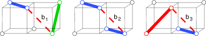
Figure 2: Types of different inter-dimer bonds depicted as dashed lines. Dimers are represented with and are colored according to three cubic planes they belong to. Bonds ${\sf b_{1}}$ and ${\sf b_{2}}$ couple dimers with perpendicular to these bonds. Bond ${\sf b_{3}}$ connects a dimer from a orthogonal plane with another one that is in the same plane as ${\sf b_{3}}$ itself.

Fig. 2 shows all possible inter-dimer bonds allowed in the ground state manifold. Such a bond may connect two dimers both perpendicular the connecting bond itself: then, either the connected dimers belong to different planes $({\sf b_{1}})$ or to the same plane $({\sf b_{2}})$. The third possibility, ${\sf b_{3}}$, is that one of the dimers is in the same plane as the inter-dimer bond, and the other is perpendicular to them [see Fig. 2]. Consequently, regardless of the dimer arrangements, each dimer has exactly six neighboring ${\sf b_{3}}$ bonds. Out of 6${\cal N}$ bonds of the fcc lattice with ${\cal N}$ sites, there are $\frac{1}{2}{\cal N}$ dimer and $3{\cal N}$ of ${\sf b_{3}}$-type bonds, thus remaining $\frac{5}{2}{\cal N}$ bonds are ${\sf b_{1}}$- or ${\sf b_{2}}$-types. Each dimer (${\sf b_{n}}$-type) bonds host a finite energy ${\cal E}_{\sf d}$ (${\cal E}_{\sf b_{n}}$). As both ${\sf b_{1}}$ and ${\sf b_{2}}$ bonds connect dimers out of their plane, ${\cal E}_{\sf b_{1}}={\cal E}_{\sf b_{2}}$ and the energy of a product dimer state

$${\sf E}_{\sf DS}=\bigl{(}{\cal E}_{\sf d}+5{\cal E}_{\sf b_{1}}+6{\cal E}_{\sf b_{3}}\bigr{)}{\cal N}/2$$ (6)

is independent of the dimer covering. Hence, the inter-dimer couplings do not order dimers and the massive orientational degeneracy persists. In real materials, however, a mis-site disorder and/or uncorrelated local distortions most likely select a random dimer covering, rendering the system to freeze in a glassy manner.

In an amorphous dimer-singlet phase, momenta of the excitations are not well defined, but their energies are. Moreover, the inter-dimer couplings are much smaller than the intra-dimer exchange, allowing isolated dimer description of the bulk magnetic spectra. At $\eta,\lambda=0$, as product dimer states are exact eigenstates, spins of different dimers are completely decoupled. In the large $\lambda$ limit, the inter-dimer pseudo-spin exchange ${J}^{\prime}\simeq\frac{1}{16}{\tilde{J}}\ll{\tilde{J}}$. This estimate follows from Eq. (3) by noting that $\langle\tilde{P}_{ij}^{(\gamma)}\rangle=\frac{1}{16}$ on the inter-dimer bonds. Two types of local excitations allowed by magnetic dipole transitions are illustrated in Fig. 3. The upper one corresponds to flipping locally a (pseudo-)spin at the energy cost $\Delta_{\text{S}}=J\;({\tilde{J}})$ in small (large) $\lambda$ limit. The lower is a (pseudo-)orbital excitation that costs half the energy, $\Delta_{\text{O}}=\frac{1}{2}J\;(\frac{1}{2}{\tilde{J}})$, of a spin-like excitation. These estimates follow from the expectation values of the limiting Hamiltonians Eqs.(2,3) in the ground state of an isolated bond, Fig. 3(left), and its excited states, Fig. 3(right). Using reported parameters for Ba₂YMoO₆ tU , we estimate energy of spin-like (orbital-like) excitations $\Delta_{\text{S(O)}}\simeq 20-45\;(10-23)$ meV, for large$-$small SOC, and their bandwidth ($\sim J^{\prime}$) of about few meV. In the magnetic dipolar channel, spin-like excitations carry stronger intensity than orbital-like ones. These findings agree well with neutron scattering data on powder samples discussed below.

There are additional thermally accessible non-local excitations at lower energies. For example AF coupled spin clusters, or orphan spins may emerge as a result of thermally induced orbital reorientation. An important difference between the well studied spin-only dimer systems and our model is the lack of a hard-gap. Here, on account of orbital degrees of freedom, the spectrum cannot be characterized by a single energy scale.

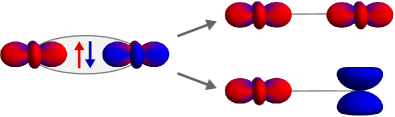
Figure 3: Excitations of a spin-orbit dimer in the large $\lambda$ limit. Flipping locally, for example, the $j^{z}=-1/2$ component to $j^{z}=1/2$ or to $j^{z}=-3/2$ corresponds to flipping the pseudo-spin (top) or pseudo-orbital (bottom), respectively. Local excitations for small SOC correspond to changing the real spins or orbitals.

Phase diagram.– To explore the entire phase diagram of the full Hamiltonian (1), we used a site-factorized variational approach and compared the energies of ordered and dimer-singlet phases. The latter is numerically obtained from Eq. (6) using a product state of the exact wave-functions of isolated dimers. Within our variational approach, the magnetic and crystallographic unit cells coincide, however, we still need forty variational parameters to construct a trial wave-function SM . When $\eta=0$ the ground state is a random arrangement of spin-orbit dimers [see inset in Fig. 4] for any value of $\lambda$. Only the nature of pseudo-spins forming the singlet dimers is affected by $\lambda$, in accordance with the above analytical considerations. For large enough Hund’s coupling, we find two non-collinear but coplanar phases of ordered total angular momenta ${\vec{j}}$ [see Fig. 4]. One, termed here as coplanar-F, has finite net moment along $[110]$ (or equivalent) direction, i.e. along one of the NN bond, as experimentally observed Stitzer et al. (2002). The other, coplanar-AF, has no net moment. In the dimer-singlet phase, on a dimer bond in $\gamma$-plane corresponding $\gamma$-orbital is predominately occupied, with occupancy decreasing from $n^{(\gamma)}=1$ to $\frac{2}{3}$ with increasing $\lambda$. Hunds coupling induced transitions to ordered states are accompanied by complex rearrangements of an electron density within SOC split $t_{2g}$-multiplet, with orbital occupancies dictated by the actual values of parameters, e.g. in coplanar-AF order in a cubic $\gamma$-plane the $\alpha$- and $\beta$-orbitals are predominantly occupied compared to the in-plane $\gamma$-orbital. All phase boundaries appear to be first order within our approach: the net moment and the order parameters drop to zero across the transitions from coplanar-F to coplanar-AF state and from the ordered to disordered dimer-singlet phase, respectively. However, one cannot rule out a second order symmetry allowed transition between ordered states, or an exotic continuous transition from spontaneously dimerized phase to ordered states Senthil et al. (2004).

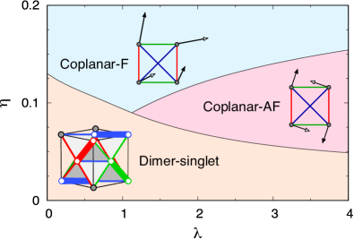
Figure 4: Phase diagram of the model (1) as the function of Hund’s coupling $\eta$ and the SOC $\lambda$ (in units of $J$). For small values of $\eta$ the dimer-singlet phase (see inset) is stable over the entire range of $\lambda$. With increasing Hund’s coupling, non-collinear coplanar phases with ordered moments in one of the cubic planes are stabilized. The ferro-type coplanar state, coplanar-F, has a finite net moment pointing along $[110]$ (or equivalent) direction. The cartoon figures show a tetrahedron of four molybdenum sites projected onto the plane of ordered ${\vec{j}}$-moments, depicted as arrows.

Experimental implications.– The dimer-singlet phase captures experimental observations on the molybdenum compounds. In agreement with experiments, it does not exhibit any long-range ordering nor breaks any global symmetry. Its extensive degeneracy explains the observed glassy behavior and suggest the presence of a residual entropy, that cannot be excluded based on heat capacity data de Vries et al. (2010). Magnetic susceptibility and electronic heat capacity de Vries et al. (2010, 2013) suggest the presence of pseudo-gapped, rather than hard-gapped, low-energy excitations, consistent with the dimer-singlet phase. Neutron scattering experiments on powder samples Carlo et al. (2011) revealed excitations that are in line with the spectrum of weakly coupled spin-orbit dimers. An intense ’mode’ observed at $\Delta_{\text{S}}\simeq 28$ meV with bandwidth of about $4$ meV is interpreted here as a (pseudo-)spin singlet-to-triplet excitation. A less intense, lower-energy ($\Delta_{\text{O}}\simeq 9-17$ meV) response centred around at half the energy of $\Delta_{\text{S}}$ is naturally attributed to (pseudo-)orbital excitation. These lower-lying excitations have also been observed in NMR response Aharen et al. (2010). The energetics of the observed excitations agrees well with above estimates $\Delta_{\text{S(O)}}\simeq 20-45\;(10-23)$ meV. In addition, the infrared transmission spectra indicate the emergence of uncorrelated local distortions of MoO₆ octahedra below 130 K Qu et al. (2013), at around the same temperature the magnetic susceptibility start to decrease, most likely due to formation of spin-orbit dimers. In the dimer-singlet phase, such uncorrelated distortions emerge due to the directional character of the occupied orbitals.

The four-sublattice ordered states in the phase diagram (Fig. 4) may provide description for the iso-structural osmium compounds, Ba₂LiOsO₆ and Ba₂NaOsO₆. The latter is characterized by very small net magnetic moment $\sim\!0.2\mu_{\rm B}$ along $[110]$ easy axis Stitzer et al. (2002). We find the net moment $\vec{M}=2\vec{S}-\vec{l}$ along the same $[110]$ (or equivalent) direction, being $\sim 1\mu_{B}$ for small and $\sim 0.1\mu_{B}$ for large $\lambda$.

To summarize, within a minimal microscopic model, we have proposed unified theoretical description of possible ground states in $d^{1}$ cubic double perovskites. The obtained spin-orbital model shows a rich phase behavior including a massively degenerate dimer-singlet manifold, without any long-range order, and unusual non-collinear ordered patterns. Our theoretical study elucidates physics behind and provides explanations of experimental data on molybdenum and osmium based compounds. The physics discussed here may also be relevant to other heavy transition metal compounds, such as molybdenum pyrochlores, in which random distribution of ‘dimerized’ bonds, induced by orbital degrees, have been recently revealed by pair-distribution function measurements Thygesen et al. (2017).

We thank G. Chen, M. Haverkort, G. Khaliullin, F. Mila, W. Natori, J.A.M. Paddison, S. Streltsov, and H. Takagi for discussions. J.R. acknowledges funding from the Hungarian OTKA grant K106047. Work by L.B. was supported by the DOE, Office of Science, Basic Energy Sciences under award number DE-FG02-08ER46524. G.J. benefitted from the facilities of the KITP, and was supported in part by the NSF under Grant No. NSF PHY11-25915.

Supplemental Material:
“Spin-Orbit Dimers and Non-Collinear Phases in $d^{1}$ Cubic Double Perovskites”

.1 Spin-orbital superexchange

The first three terms of the model (1) in main text describe spin exchange couplings depending on the orbital occupancy and exemplifies a version of Goodenough-Kanamori rules. Three possible orbital configurations of a bond are shown in Fig. S1(a). The strongest, antiferromagnetic (AF), exchange is achieved when the lobs of occupied orbitals on both neighboring sites point along the bond in between (see Fig. S1(a)[left]), and is given by $J_{3}$ term in Eq. (1). When only one occupied orbital is directed along the bond, Fig. S1(a)[middle], the spin exchange could be either ferromagnetic (FM) or AF, $J_{1}$ and $J_{2}$ terms in Eq. (1), respectively. The Hunds coupling induced splitting of virtual doubly occupied state favors the high spin, $S=1$, configuration and resulting FM exchange is stronger than AF one, $J_{1}>J_{2}$. In the limit of zero Hund’s coupling, $J_{1}=J_{2}$ and spin exchange on such a bond vanishes. When both sites are occupied by orbitals directed away from the common bond, Fig. S1(a)[right], there is no virtual hopping process along that bond, hence no exchange and energy gain.

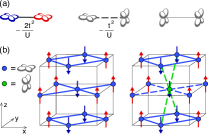
Figure S1: (a) Nearest-neighbor bonds of $\gamma$-type have zero energy unless one of the electrons occupies $\gamma$-orbital. The energy gain is maximal when both orbitals correspond to the plane of the bond. (b) The classical ground state is orbitally ordered antiferromagnetic state of decoupled layers (left). Flipping locally an orbital ‘flavor’ does not cost any energy. Although, the bond energies in $xy$-plane are halved, there are new exchange paths to the lower and upper layers (right).

.2 The limit of zero Hunds coupling

In the limit $\eta=0$, we are left with the only one exchange scale $J=4t^{2}/U$, and exchange couplings become $J_{3}=4J_{2}=4J_{1}=J$. The exchange part of Eq. (1) can then be simplified, by using identities

$$\sum_{\gamma}n_{i}^{\gamma}=1~{},\;\sum_{{\langle ij\rangle}_{\gamma}}{\bigr{(}{P}_{ij}^{(\gamma)}+\bar{P}_{ij}^{(\gamma)}\bigl{)}}=-\sum_{{\langle ij\rangle}_{\gamma}}\bar{P}_{ij}^{(\gamma)}+4\cal{N}~{},$$

$$\text{to the form}\;\;\mathcal{H}=J\sum_{{\langle ij\rangle}_{\gamma}}{\bigr{(}}\vec{S}_{i}\cdot\vec{S}_{j}+\frac{1}{4}{\bigl{)}}\bar{P}_{ij}^{(\gamma)}~{}.$$ (S1)

The classical, site-factorized, ground state manifold of the above Hamiltonian has an extensive degeneracy due to orbital degrees of freedom. One of the classical states of the model (S1) on the fcc lattice is built of decoupled antiferromagnetic layers as shown in Fig. S1(b). On the nearest-neighbor bonds of each layer, the expectation value $\langle{\vec{S}}_{i}\cdot{\vec{S}}_{j}\rangle=-\frac{1}{4}$ setting the spin part in Eq. (S1) to zero. The ground state energy is then a constant, independent of orbital configurations. Hence, one can locally flip an orbital flavour without changing energy [see Fig. S1(b)] and generate macroscopically degenerate classical ground state manifold.

.3 Exact solution of a two-site problem

To investigate the dimer-factorized solution we begin with the case of an isolated bond, e.g. in $xy$-plane ($c$-type bond). The exact ground state wave-function, from numerical diagonalization of the model (1) of main text, at any values of the spin-orbit coupling $\lambda$, can be written as linear a combination of two kinds of spin-orbit singlets. The dominant singlet in this linear combination is $\left|\leavevmode\hbox to17.47pt{\vbox to6.09pt{\text{[drawing]}}}\right>$ of Eq. (4) with pseudo-spins introduced in Eq. (5) of the main text. Contribution from the other singlet vanishes in the limiting cases $\lambda=0$ and $\lambda\to\infty$ and is negligibly small for any value of $\lambda$. Thus, the ground state is approximately a pure singlet of Eq. (4). To see how close the trial singlet state (4) is to the exact dimer ground state we plot the overlap between them in Fig. S2.

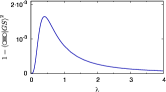
Figure S2: Overlap between the exact dimer ground state and the singlet $\left|\leavevmode\hbox to17.47pt{\vbox to6.09pt{\text{[drawing]}}}\right>$ (4) introduced in the main text. For arbitrary value of $\lambda$, $\left|\leavevmode\hbox to17.47pt{\vbox to6.09pt{\text{[drawing]}}}\right>$ remains extremely close to the exact solution.

.4 Extensive degeneracy of constrained dimer coverings

In the following, we show that in spite of the constraint that do not allow two neighbouring dimers to be in the same plane (‘no-plane’ constraint), there is infinite number of dimer configurations of which the system chooses upon freezing into a glassy disordered phase. Let us consider the $[111]$-planes of the fcc lattice which naturally contains all three types of bonds ($a$, $b$ and $c$) as shown in Fig. S3(a). The fcc lattice can be viewed as stacked layers of triangular lattice, where these layers are the $[111]$ planes and the three sides of the triangles correspond to the three kinds of bonds [see Fig. S3(b)]. A possible dimer-product state is to cover a layer with stripes of two kinds of dimers and repeat the pattern in the neighboring layers so that the different dimers alternate on top of each other. Two consecutive layers of such a dimer configuration is illustrated in Fig. S3(c). For convenience we denoted the top layer with bright, and the bottom layer with dim colors. It is easy to see that changing the dimer state of four neighboring sites within a layer does not violate the ‘no-plane’ constrain and hence, does not change the ground state energy. Such a flip is illustrated in Fig. S3(d). As we can flip anywhere, even successively at more than one plaquette of four sites, there are an extensive number of possible dimer coverings.

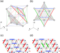
Figure S3: (color online) (a) and (b) illustrate two neighboring $[111]$-planes of the fcc lattice indicated with black and white sites. (c) A possible covering of fcc lattice with $b$-type (red) and $c$-type (blue) ‘orthogonal’ dimers. The two layers depicted here are denoted with grey and white sites. The solid and dashed lines correspond to intra and inter layer bonds, respectively. (d) Switching the dimers on four neighboring sites in a given layer does not violate the ‘no-plane’ constraint and does not effect the ground state energy.

.5 Variational approach

To compare the dimer-singlet solution with other possible phases we performed site-factorized variational calculations. We look for phases which have a unit cell equivalent to the crystallographic one, and as such, our variational approach cannot describe incommensurate orderings or patterns with larger unit cell. As pointed out in the main text, the local Hilbert space of a molybdenum site consists of the six states of a t${}_{2g}^{1}$-configuration. Namely, $|\pm 1,\sigma\rangle$ and $|0,\sigma\rangle$, with spin variables $\sigma=\uparrow$ or $\downarrow$. For simplicity, let us denote these states in the following way; $|1,\uparrow\rangle,\cdots,|-1,\downarrow\rangle=|\phi\rangle_{1},\cdots,|\phi\rangle_{6}$.

In order to find the most general site-factorized solution we chose our local variational wave function to be

$$|\psi_{i}\rangle=\sum_{n=1}^{6}\zeta_{n}|\phi_{i}\rangle_{n}\;,$$ (S2)

where $\zeta_{n}$ are complex parameters and the index $i$ denotes the sites. Actually, we only need ten real parameters per molybdenum site and can for example set $\zeta_{1}=1$. The complex coefficients of six state would give 12 real parameters, but due to normalization and a variable global phase we are left with ten independent real parameters.

As there are four Mo ions in the unit cell of the fcc lattice we have all together 40 variational parameters in the site-factorized wave function $\prod_{i=1}^{4}|\psi_{i}\rangle$. Taking all 24 direction-dependent bonds of the unit cell as well as the spin-orbit coupling into account, we minimize the energy for these 40 variational parameters and compare it to the spin-orbital dimer-singlet solution. The resulting phase diagram is shown in Fig. 4 of the main text.

References

- Balents (2010) L. Balents, Nature 464, 199 (2010).
- Savary and Balents (2016) L. Savary and L. Balents, ArXiv e-prints (2016), arXiv:1601.03742 [cond-mat.str-el] .
- Kugel and Khomskii (1982) K. Kugel and D. Khomskii, Sov. Phys. Usp. 25, 231 (1982).
- Khaliullin (2005) G. Khaliullin, Prog. Theor. Phys. Suppl. 160, 155 (2005).
- Pen et al. (1997) H. F. Pen, J. van den Brink, D. I. Khomskii, and G. A. Sawatzky, Phys. Rev. Lett. 78, 1323 (1997).
- Khaliullin and Maekawa (2000) G. Khaliullin and S. Maekawa, Phys. Rev. Lett. 85, 3950 (2000).
- Vernay et al. (2004) F. Vernay, K. Penc, P. Fazekas, and F. Mila, Phys. Rev. B 70, 014428 (2004).
- Di Matteo et al. (2004) S. Di Matteo, G. Jackeli, C. Lacroix, and N. B. Perkins, Phys. Rev. Lett. 93, 077208 (2004).
- Di Matteo et al. (2005) S. Di Matteo, G. Jackeli, and N. B. Perkins, Phys. Rev. B 72, 024431 (2005).
- Jackeli and Khomskii (2008) G. Jackeli and D. Khomskii, Phys. Rev. Lett. 100, 147203 (2008).
- Chen and Balents (2008) G. Chen and L. Balents, Phys. Rev. B 78, 094403 (2008).
- Jackeli and Khaliullin (2009) G. Jackeli and G. Khaliullin, Phys. Rev. Lett. 102, 017205 (2009).
- Chen et al. (2010) G. Chen, R. Pereira, and L. Balents, Phys. Rev. B 82, 174440 (2010).
- Stitzer et al. (2002) K. Stitzer, M. Smith, and H.-C. zur Loye, Solid State Sciences 4, 311 (2002).
- Erickson et al. (2007) A. Erickson, S. Misra, G. Miller, R. Gupta, Z. Schlesinger, W. Harrison, J. Kim, and I. Fisher, Phys. Rev. Lett. 99, 016404 (2007).
- Steele et al. (2011) A. Steele, P. Baker, T. Lancaster, F. Pratt, I. Franke, S. Ghannadzadeh, P. Goddard, W. Hayes, D. Prabhakaran, and S. Blundell, Phys. Rev. B 84, 144416 (2011).
- Lee and Pickett (2007) K.-W. Lee and W. E. Pickett, Europhys. Lett. 80, 37008 (2007).
- Gangopadhyay and Pickett (2015) S. Gangopadhyay and W. Pickett, Phys. Rev. B 91, 045133 (2015).
- Gangopadhyay and Pickett (2016) S. Gangopadhyay and W. E. Pickett, Phys. Rev. B 93, 155126 (2016).
- Lu et al. (2017) L. Lu, M. Song, W. Liu, A. P. Reyes, P. Kuhns, H. O. Lee, I. R. Fisher, and V. F. Mitrović, Nature Communications 8, 14407 EP (2017).
- Aharen et al. (2010) T. Aharen, J. Greedan, C. Bridges, A. Aczel, J. Rodriguez, G. MacDougall, G. Luke, T. Imai, V. Michaelis, S. Kroeker, H. Zhou, C. Wiebe, and L. Cranswick, Phys. Rev. B 81, 224409 (2010).
- de Vries et al. (2010) M. de Vries, A. Mclaughlin, and J.-W. Bos, Phys. Rev. Lett. 104, 177202 (2010).
- de Vries et al. (2013) M. de Vries, J. Piatek, M. Misek, J. Lord, H. Rønnow, and J.-W. G. Bos, New Journal of Physics 15, 043024 (2013).
- Mclaughlin et al. (2010) A. Mclaughlin, M. de Vries, and J.-W. Bos, Phys. Rev. B 82, 094424 (2010).
- Coomer and Cussen (2013) F. Coomer and E. Cussen, Journal of Physics: Condensed Matter 25, 082202 (2013).
- Natori et al. (2016) W. Natori, E. Andrade, E. Miranda, and R. Pereira, Phys. Rev. Lett. 117, 017204 (2016).
- Abragam and Bleaney (1970) A. Abragam and B. Bleaney, Electron Paramagnetic Resonance of Transition Ions (Clarendon Press, Oxford, 1970).
- (28) Recent ab-initio study of Ba2YMoO6 suggests eV and order of magnitude smaller NN off-diagonal as well as further neighbor hopping amplitudes, S. Streltsov (privet communication).
- (29) The parameters eV Erickson et al. (2007); Str and eV Erickson et al. (2007); Vaugier et al. (2012) have been suggested for molybdenum and osmium double perovskites. We thus estimate that is small enough to justify our perturbative expansion up to the leading order.
- (30) , and .
- (31) See supplemental material at [URL] for the details.
- Jackeli and Ivanov (2007) G. Jackeli and D. A. Ivanov, Phys. Rev. B 76, 132407 (2007).
- (33) Similar representation has been used in Ref. Natori et al., 2016.
- Senthil et al. (2004) T. Senthil, A. Vishwanath, L. Balents, S. Sachdev, and M. P. A. Fisher, Science 303, 1490 (2004).
- Carlo et al. (2011) J. P. Carlo, J. P. Clancy, T. Aharen, Z. Yamani, J. P. C. Ruff, J. J. Wagman, G. J. Van Gastel, H. M. L. Noad, G. E. Granroth, J. E. Greedan, H. A. Dabkowska, and B. D. Gaulin, Phys. Rev. B 84, 100404 (2011).
- Qu et al. (2013) Z. Qu, Y. Zou, S. Zhang, L. Ling, L. Zhang, and Y. Zhang, Journal of Applied Physics 113, 17E137 (2013).
- Thygesen et al. (2017) P. M. M. Thygesen, J. A. M. Paddison, R. Zhang, K. A. Beyer, K. W. Chapman, H. Y. Playford, M. G. Tucker, D. A. Keen, M. A. Hayward, and A. L. Goodwin, Phys. Rev. Lett. 118, 067201 (2017).
- Vaugier et al. (2012) L. Vaugier, H. Jiang, and S. Biermann, Phys. Rev. B 86, 165105 (2012).

References

- Balents (2010) L. Balents, Nature 464, 199 (2010).
- Savary and Balents (2016) L. Savary and L. Balents, ArXiv e-prints (2016), arXiv:1601.03742 [cond-mat.str-el] .
- Kugel and Khomskii (1982) K. Kugel and D. Khomskii, Sov. Phys. Usp. 25, 231 (1982).
- Khaliullin (2005) G. Khaliullin, Prog. Theor. Phys. Suppl. 160, 155 (2005).
- Pen et al. (1997) H. F. Pen, J. van den Brink, D. I. Khomskii, and G. A. Sawatzky, Phys. Rev. Lett. 78, 1323 (1997).
- Khaliullin and Maekawa (2000) G. Khaliullin and S. Maekawa, Phys. Rev. Lett. 85, 3950 (2000).
- Vernay et al. (2004) F. Vernay, K. Penc, P. Fazekas, and F. Mila, Phys. Rev. B 70, 014428 (2004).
- Di Matteo et al. (2004) S. Di Matteo, G. Jackeli, C. Lacroix, and N. B. Perkins, Phys. Rev. Lett. 93, 077208 (2004).
- Di Matteo et al. (2005) S. Di Matteo, G. Jackeli, and N. B. Perkins, Phys. Rev. B 72, 024431 (2005).
- Jackeli and Khomskii (2008) G. Jackeli and D. Khomskii, Phys. Rev. Lett. 100, 147203 (2008).
- Chen and Balents (2008) G. Chen and L. Balents, Phys. Rev. B 78, 094403 (2008).
- Jackeli and Khaliullin (2009) G. Jackeli and G. Khaliullin, Phys. Rev. Lett. 102, 017205 (2009).
- Chen et al. (2010) G. Chen, R. Pereira, and L. Balents, Phys. Rev. B 82, 174440 (2010).
- Stitzer et al. (2002) K. Stitzer, M. Smith, and H.-C. zur Loye, Solid State Sciences 4, 311 (2002).
- Erickson et al. (2007) A. Erickson, S. Misra, G. Miller, R. Gupta, Z. Schlesinger, W. Harrison, J. Kim, and I. Fisher, Phys. Rev. Lett. 99, 016404 (2007).
- Steele et al. (2011) A. Steele, P. Baker, T. Lancaster, F. Pratt, I. Franke, S. Ghannadzadeh, P. Goddard, W. Hayes, D. Prabhakaran, and S. Blundell, Phys. Rev. B 84, 144416 (2011).
- Lee and Pickett (2007) K.-W. Lee and W. E. Pickett, Europhys. Lett. 80, 37008 (2007).
- Gangopadhyay and Pickett (2015) S. Gangopadhyay and W. Pickett, Phys. Rev. B 91, 045133 (2015).
- Gangopadhyay and Pickett (2016) S. Gangopadhyay and W. E. Pickett, Phys. Rev. B 93, 155126 (2016).
- Lu et al. (2017) L. Lu, M. Song, W. Liu, A. P. Reyes, P. Kuhns, H. O. Lee, I. R. Fisher, and V. F. Mitrović, Nature Communications 8, 14407 EP (2017).
- Aharen et al. (2010) T. Aharen, J. Greedan, C. Bridges, A. Aczel, J. Rodriguez, G. MacDougall, G. Luke, T. Imai, V. Michaelis, S. Kroeker, H. Zhou, C. Wiebe, and L. Cranswick, Phys. Rev. B 81, 224409 (2010).
- de Vries et al. (2010) M. de Vries, A. Mclaughlin, and J.-W. Bos, Phys. Rev. Lett. 104, 177202 (2010).
- de Vries et al. (2013) M. de Vries, J. Piatek, M. Misek, J. Lord, H. Rønnow, and J.-W. G. Bos, New Journal of Physics 15, 043024 (2013).
- Mclaughlin et al. (2010) A. Mclaughlin, M. de Vries, and J.-W. Bos, Phys. Rev. B 82, 094424 (2010).
- Coomer and Cussen (2013) F. Coomer and E. Cussen, Journal of Physics: Condensed Matter 25, 082202 (2013).
- Natori et al. (2016) W. Natori, E. Andrade, E. Miranda, and R. Pereira, Phys. Rev. Lett. 117, 017204 (2016).
- Abragam and Bleaney (1970) A. Abragam and B. Bleaney, Electron Paramagnetic Resonance of Transition Ions (Clarendon Press, Oxford, 1970).
- (28) Recent ab-initio study of Ba2YMoO6 suggests eV and order of magnitude smaller NN off-diagonal as well as further neighbor hopping amplitudes, S. Streltsov (privet communication).
- (29) The parameters eV Erickson et al. (2007); Str and eV Erickson et al. (2007); Vaugier et al. (2012) have been suggested for molybdenum and osmium double perovskites. We thus estimate that is small enough to justify our perturbative expansion up to the leading order.
- (30) , and .
- (31) See supplemental material at [URL] for the details.
- Jackeli and Ivanov (2007) G. Jackeli and D. A. Ivanov, Phys. Rev. B 76, 132407 (2007).
- (33) Similar representation has been used in Ref. Natori et al., 2016.
- Senthil et al. (2004) T. Senthil, A. Vishwanath, L. Balents, S. Sachdev, and M. P. A. Fisher, Science 303, 1490 (2004).
- Carlo et al. (2011) J. P. Carlo, J. P. Clancy, T. Aharen, Z. Yamani, J. P. C. Ruff, J. J. Wagman, G. J. Van Gastel, H. M. L. Noad, G. E. Granroth, J. E. Greedan, H. A. Dabkowska, and B. D. Gaulin, Phys. Rev. B 84, 100404 (2011).
- Qu et al. (2013) Z. Qu, Y. Zou, S. Zhang, L. Ling, L. Zhang, and Y. Zhang, Journal of Applied Physics 113, 17E137 (2013).
- Thygesen et al. (2017) P. M. M. Thygesen, J. A. M. Paddison, R. Zhang, K. A. Beyer, K. W. Chapman, H. Y. Playford, M. G. Tucker, D. A. Keen, M. A. Hayward, and A. L. Goodwin, Phys. Rev. Lett. 118, 067201 (2017).
- Vaugier et al. (2012) L. Vaugier, H. Jiang, and S. Biermann, Phys. Rev. B 86, 165105 (2012).