The accumulated persistence function, a new useful functional summary statistic for topological data analysis, with a view to brain artery trees and spatial point process applications

Abstract

We start with a simple introduction to topological data analysis where the most popular tool is called a persistent diagram. Briefly, a persistent diagram is a multiset of points in the plane describing the persistence of topological features of a compact set when a scale parameter varies. Since statistical methods are difficult to apply directly on persistence diagrams, various alternative functional summary statistics have been suggested, but either they do not contain the full information of the persistence diagram or they are two-dimensional functions. We suggest a new functional summary statistic that is one-dimensional and hence easier to handle, and which under mild conditions contains the full information of the persistence diagram. Its usefulness is illustrated in statistical settings concerned with point clouds and brain artery trees. The appendix includes additional methods and examples, together with technical details. The R-code used for all examples is available at http://people.math.aau.dk/~christophe/Rcode.zip.

Keywords: clustering, confidence region, global rank envelope, functional boxplot, persistent homology, two-sample test.

1 Introduction

Statistical methods that make use of algebraic topological ideas to summarize and visualize complex data are called topological data analysis (TDA). In particular persistent homology and a method called the persistence diagram are used to measure the persistence of topological features. As we expect many readers may not be familiar with these concepts, Section 1.1 discusses two examples without going into technical details though a few times it is unavoidable to refer to the terminology used in persistent homology. Section 1.2 discusses the use of the persistence diagram and related summary statistics and motivates why in Section 1.3 a new functional summary statistic called the accumulative persistence function (APF) is introduced. The remainder of the paper demonstrates the use of the APF in various statistical settings concerned with point clouds and brain artery trees.

1.1 Examples of TDA

The mathematics underlying TDA uses technical definitions and results from persistent homology, see Fasy et al. (2014) and the references therein. This theory will not be needed for the present paper. Instead we provide an understanding through examples of the notion of persistence of $k$-dimensional topological features for a sequence of compact subsets $C_{t}$ of the $d$-dimensional Euclidean space $\mathbb{R}^{d}$, where $t\geq 0$, $k=0,1,\ldots,d-1$, and either $d=2$ (Section 1.1.1) or $d=3$ (Section 1.1.2). Recalling that a set $A\subseteq\mathbb{R}^{d}$ is path-connected if any two points in $A$ are connected by a curve in $A$, a $0$-dimensional topological feature of a compact set $C\subset\mathbb{R}^{d}$ is a maximal path-connected subset of $C$, also called a connected component of $C$. The meaning of a $1$-dimensional topological feature is simply understood when $d=2$, and we appeal to this in a remark at the end of Section 1.1.1 when $d=3$.

1.1.1 A toy example

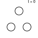
Let $C\subset\mathbb{R}^{2}$ be the union of the three circles depicted in the top-left panel of Figure 1. The three circles are the $0$-dimensional topological features (the connected components) of $C$, as any curve that goes from a circle to another will be outside $C$. The complement $\mathbb{R}^{2}\setminus S$ has four connected components, one of which is unbounded, whilst the three others are the $1$-dimensional topological features of $C$, also called the loops of $C$ (the boundary of each bounded connected component is a closed curve with no crossings; in this example the closed curve is just a circle).

Figure 1: The four first panels show a simple example of spherically growing circles centred at (-1,-1), (1,-1), and (0,1) and all with radii 0.5 when time is $0$. The fifth panel shows the persistence diagram for the connected components ($k=0$) and the loops ($k=1$). The final panel shows the corresponding accumulated persistence functions.

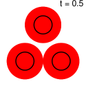
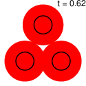
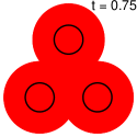
For $t\geq 0$, let $C_{t}$ be the subset of points in $\mathbb{R}^{2}$ within distance $t$ from $C$. Thinking of $t$ as time, $C_{t}$ results when each point on $C$ grows as a disc with constant speed one. The algebraic topology (technically speaking the Betti numbers) changes exactly at the times $t=0,0.5,0.62,0.75$, see the first four panels of Figure 1: For each topological dimension $k=0,1$, let $t_{i}^{(k)}$ denote the time of the $i$th change. First, $C_{0}=C$ has three connected components and three loops as given above; we say that they are born at time $t_{1}^{(0)}=t_{1}^{(1)}=0$ (imaging there was nothing before time 0). Second, the loops disappear and two connected components merge into one connected component; we say that the loops and one of the connected components die at time $t_{2}^{(0)}=t_{2}^{(1)}=0.5$; since the two merging connected components were born at the same time, it is decided uniformly at random which one should die respectively survive; the one which survives then represent the new merged connected component. Third, at time $t_{3}^{(0)}=t_{3}^{(1)}=0.62$, a new loop is born and the two connected component merge into one which is represented by the oldest (first born) connected component whilst the other connected component (the one which was retained when the two merged at time $t_{2}^{(0)}=0.5$) dies; the remaining connected component "lives forever" after time $0.62$ and it will be discarded in our analysis. Finally, at time $t_{4}^{(1)}=0.75$, the loop dies.

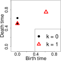
Hence, for each $k=0,1$, there is a multiset of points specifying the appearance and disappearance of each $k$-dimensional topological feature as $t$ grows. A scatter plot of these points is called a persistence diagram, see Figure 1 (bottom-middle panel): For $k=0$ (the connected components), the points are $(0,0.5)$ and $(0,0.62)$ (as $(0,\infty)$ is discarded from the diagram) with multiplicities 1 and 1, respectively; and for $k=1$ (the loops), the points are $(0,0.5)$ and $(0.62,0.75)$ with multiplicities 3 and 1, respectively. The term "persistence" refers to that distant connected components and large loops are present for a long time; which here of course just corresponds to the three circles/connected components of $C$ and their loops persist for long whilst the last appearing loop has a short lifetime and hence is considered as "noise".

Usually in practice $C$ is not known but a finite subset of points $\{x_{1},\ldots,x_{N}\}$ has been collected as a sample on $C$, possibly with noise. Then we redefine $C_{t}$ as the union of closed discs of radius $t$ and with centres given by the point cloud. Hence the connected components of $C_{0}$ are just the points $x_{1},\ldots,x_{N}$, and $C_{0}$ has no loops. For $t>0$, it is in general difficult to directly compute the connected components and loops of $C_{t}$, but a graph in $\mathbb{R}^{m}$ (with $m\geq 2$) can be constructed so that its connected components correspond to those of $C_{t}$ and moreover the triangles of the graph may be filled or not in a way so that the loops of the obtained triangulation correspond to those of $C_{t}$.

Remark: Such a construction can also be created in the case where $C_{t}$ is the union of $d$-dimensional closed balls of radius $t$ and with centres given by a finite point pattern $\{x_{1},\ldots,x_{N}\}\subset\mathbb{R}^{d}$. The construction is a so-called simplicial complex such as the Čech-complex, where $m$ may be much larger than $d$, or the Delaunay-complex (or alpha-complex), where $m=d$, and a technical result (the Nerve Theorem) establishes that it is possible to identify the topological features of $C_{t}$ by the Čech or Delaunay-complex, see e.g. Edelsbrunner and Harer (2010). It is unnecessary for this paper to understand the precise definition of these notions, but as $d=2$ or $d=3$ is small in our examples, it is computationally convenient to use the Delaunay-complex. When $d=3$, we may still think of a 1-dimensional topological feature as a loop, i.e. a closed curve with no crossings; again the simplicial complex is used for the "book keeping" when determining the persistence of a loop. For example, a 2-dimensional sphere has no loops, and a torus in $\mathbb{R}^{3}$ has two. Finally, when $d\geq 3$, a $k$-dimensional topological feature is a $k$-dimensional manifold (a closed surface if $k=2$) that cannot "be filled in", but for this paper we omit the precise definition since it is technical and not needed.

1.1.2 Persistent homology for brain artery trees

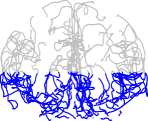
The left panel of Figure 2 shows an example of one of the 98 brain artery trees analysed in Bendich et al. (2016). The data for each tree specifies a graph in $\mathbb{R}^{3}$ consisting of a dense cloud of about $10^{5}$ vertices (points) together with the edges (line segments) connecting the neighbouring vertices; further details about the data are given in Section 2.2. As in Bendich et al. (2016), for each tree we only consider the $k$-dimensional topological features when $k=0$ or $k=1$, using different types of data and sets $C_{t}$ as described below. Below we consider the tree in Figure 2 and let $B\subset\mathbb{R}^{3}$ denote the union of its edges.

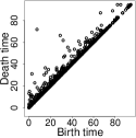
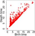
Following Bendich et al. (2016), if $k=0$, let $C_{t}=\{(x,y,z)\in B:z\leq t\}$ be the sub-level set of the height function for the tree at level $t\geq 0$ (assuming $C_{t}$ is empty for $t<0$). Thus the 0-dimensional topological features at "time/level" $t$ are the connected components of $C_{t}$. As illustrated in the left panel of Figure 2, instead of time we may think of $t$ as "water level": As the water level increases, connected components of the part of $B$ surrounded by water (the part in blue) may be born or die; we refer to this as sub-level persistence. As in Section 1.1.1, we represent the births and deaths of the connected component in a persistence diagram which is shown in Figure 2 (middle panel). The persistence of the connected components for all brain artery trees will be studied in several examples later on.

As in Bendich et al. (2016), if $k=1$, we let $B$ be represented by a point pattern $C$ of 3000 points subsampled from $B$, and redefine $C_{t}$ to be the union of balls of radii $t\geq 0$ and centres given by $C$ (as considered in the remark at the end of Section 1.1.1). The loops of $C_{t}$ are then determined by the corresponding Delaunay-complex. The right panel of Figure 2 shows the corresponding persistence diagram. The persistence of the loops for all trees will be studied in the examples to follow.

Figure 2: A brain artery tree with the "water level" indicated (left panel) and the persistence diagrams of connected components (middle panel) and loops (right pane).

1.2 Further background and objective

The persistence diagram is a popular graphical representation of the persistence of the topological features of a sequence of compact sets $C_{t}\subset\mathbb{R}^{d}$, $t\geq 0$. As exemplified above it consists for each topological dimension $k=0,\ldots,d-1$ of a multiset $\mathrm{PD}_{k}$ of points $(b_{i},d_{i})$ with multiplicities $c_{i}$, where $b_{i}$ and $d_{i}$ is a pair of birth-death times for a $k$-dimensional topological feature obtained as time $t$ grows.

In the majority of literature on TDA, including the analysis in Bendich et al. (2016) of brain artery trees, long lifetimes are of main interest whereas short lifetimes are considered as topological noise. Short lifetimes are of interest in the study of complex structures such as branch polymers and fractals, see MacPherson and Schweinhart (2012); and for brain artery trees Bendich et al. (2016) noticed in one case that "not-particularly-high persistence have the most distinguishing power in our specific application". In our examples we demonstrate that short lifetimes will also be of key interest in many situations, including when analysing the brain artery trees dataset from Bendich et al. (2016).

Chazal et al. (2013) and Chen et al. (2015) note that it is difficult to apply statistical methodology to persistent diagrams. Alternative functional summary statistics have been suggested: Bubenik (2015) introduces a sequence of one-dimensional functions called the persistent landscape, where his first function is denoted $\lambda_{1}$ and is considered to be of main interest, since it provides a measure of the dominant topological features, i.e. the longest lifetimes; therefore we call $\lambda_{1}$ the dominant function. Chazal et al. (2013) introduce the silhouette which is a weighted average of the functions of the persistent landscape, where the weights control whether the focus is on topological features with long or short lifetimes. Moreover, Chen et al. (2015) consider a kernel estimate of the intensity function for the persistent diagram viewed as a point pattern. The dominant function, the silhouette, and the intensity estimate are one-dimensional functions and hence easier to handle than the persistence diagram, however, they provide selected and not full information about the persistence diagram. In Section 1.3, we introduce another one-dimensional functional summary statistic called the accumulative persistence function and discuss its advantages and how it differs from the existing functional summary statistics.

1.3 The accumulated persistence function

For simplicity and specificity, for each topological dimension $k=0,1,\ldots,d-1$, we always assume that the persistence diagram $\mathrm{PD}_{k}=\{(b_{1},d_{1},c_{1}),\ldots,(b_{n},d_{n},c_{n})\}$ is such that $n<\infty$ and $0\leq b_{i}<d_{i}<\infty$ for $i=1,\ldots,n$. This assumption will be satisfied in our examples (at least with probability one). Often in the TDA literature, $\mathrm{PD}_{k}$ is transformed to the rotated and rescaled persistence diagram (RRPD) given by $\mathrm{RRPD}_{k}=\{(m_{1},l_{1},c_{1}),\ldots,(m_{n},l_{n},c_{n})\}$, where $m_{i}=(b_{i}+d_{i})/2$ is the meanage and $l_{i}=d_{i}-b_{i}$ is the lifetime. This transformation is useful when defining our accumulative persistence function (APF) by

$$\mathrm{APF}_{k}(m)=\sum_{i=1}^{n}c_{i}l_{i}1(m_{i}\leq m),\quad m\geq 0,$$ (1)

where $1(\cdot)$ is the indicator function and we suppress in the notation that $\mathrm{APF}_{k}$ is a function of $\mathrm{RRPD}_{k}$. The remainder of this section comments on this definition.

Formally speaking, when $\mathrm{RRPD}_{k}$ is considered to be random, it is viewed as a finite point process with multiplicities, see e.g. Daley and Vere-Jones (2003). It what follows it will always be clear from the context whether $\mathrm{PD}_{k}$ and $\mathrm{RRPD}_{k}$ are considered as being random or observed, and hence whether $\mathrm{APF}_{k}$ is a deterministic or random function. In the latter case, because $\mathrm{APF}_{k}(m)$ is an accumulative function, its random fluctuations typically increase as $m$ increases.

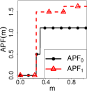
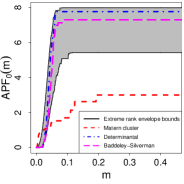
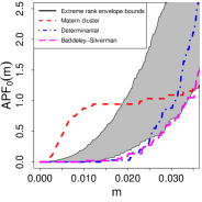
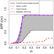
Depending on the application, the jumps and/or the shape of $\mathrm{APF}_{k}$ may be of interest as demonstrated later in our examples. A large jump of $\mathrm{APF}_{k}$ corresponds to a large lifetime (long persistence). In the simple example shown in Figure 1, both jumps of $\mathrm{APF}_{0}$ are large and indicate the three connected components (circles), whilst only the first jump of $\mathrm{APF}_{1}$ is large and indicates the three original loops. For the more complicated examples considered in the following it may be hard to recognize the individual jumps. In particular, as in the remark at the end of Section 1.1.1, suppose $C_{t}$ is the union of $d$-dimensional balls of radius $t$ and with centres given by a finite point pattern $\{x_{1},\ldots,x_{N}\}\subset\mathbb{R}^{d}$. Roughly speaking we may then have the following features as illustrated later in Example 1. For small meanages $m$, jumps of $\mathrm{APF}_{0}(m)$ correspond to balls that merge together for small values of $t$. Thus, if the point pattern is aggregated (e.g. because of clustering), we expect that $\mathrm{APF}_{0}(m)$ has jumps and is hence large for small meanages $m$, whilst if the point pattern is regular (typically because of inhibition between the points), we expect the jumps of $\mathrm{APF}_{0}(m)$ to happen and to be large for modest values of $m$ (as illustrated later in the middle panel of Figure 3 considering curves for the Matérn cluster process and the determinantal point process). For large meanages, jumps of $\mathrm{APF}_{0}(m)$ are most likely to happen in the case of aggregation. Accordingly, the shape of $\mathrm{APF}_{0}$ can be very different for these two cases (as illustrated in the first panel of Figure 3). Similar considerations lead us to expect different shapes of $\mathrm{APF}_{1}$ for different types of point patterns; we expect that $\mathrm{APF}_{1}(m)$ is large respective small for the case of aggregation respective regularity when $m$ is small, and the opposite happens when $m$ is large (as illustrated in the last panel of Figure 3).

Clearly, $\mathrm{RRPD}_{k}$ is in one-to-one correspondence to $\mathrm{PD}_{k}$. In turn, if all $c_{i}=1$ and the $m_{i}$ are pairwise distinct, then there is a one-to-one correspondence between $\mathrm{RRPD}_{k}$ and its corresponding $\mathrm{APF}_{k}$. For $k=0$, this one-to-one correspondence would easily be lost if we had used $b_{i}$ in place of $m_{i}$ in (1). We need to be careful with not over-stating this possible one-to-one correspondence. For example, imagine we want to compare two APFs with respect to $L^{q}$-norm ($1\leq q\leq\infty$) and let $\mathrm{PD}_{k}^{(1)}$ and $\mathrm{PD}_{k}^{(2)}$ be the underlying persistence diagrams. However, when points $(b,d)$ close to the diagonal are considered as topological noise (see Section 1.1.1), usually the so-called bottleneck distance $W_{\infty}(\mathrm{PD}_{k}^{(1)},\mathrm{PD}_{k}^{(2)})$ is used, see e.g. Fasy et al. (2014). Briefly, for $\epsilon>0$, let $\mathcal{N}=\{(b,d):\,b\leq d,\,l\leq 2\epsilon\}$ be the set of points at distance $\sqrt{2}\epsilon$ of the diagonal in the persistence diagram, and let $S(b,d)=\{(x,y):\,|x-b|\leq\epsilon,\,|y-d|\leq\epsilon\}$ be the square with center $(b,d)$, sides parallel to the $b$- and $d$-axes, and of side length $2\epsilon$. Then $W_{\infty}(\mathrm{PD}_{k}^{(1)},\mathrm{PD}_{k}^{(2)})\leq\epsilon$ if $\mathrm{PD}_{k}^{(2)}$ has exactly one point in each square $S(b_{i},d_{i})$, with $(b_{i},d_{i})$ a point of $\mathrm{PD}_{k}^{(1)}$ (repeating this condition $c_{i}$ times). However, small values of $W_{\infty}(\mathrm{PD}_{k}^{(1)},\mathrm{PD}_{k}^{(2)})$ does not correspond to closeness of the two corresponding APFs with respect to $L^{q}$-norm.

Note that the dominant function, the silhouette, and the intensity estimate (see Section 1.2) are in general not in a one-to-one correspondence with $\mathrm{RRPD}_{k}$. Like these functions, $\mathrm{APF}_{k}$ is a one-dimensional function, and so it is easier to handle than the sequence of functions for the persistent landscape in Bubenik (2015) and the intensity estimate in Chen et al. (2015) — e.g. confidence regions become easier to plot. Contrary to the dominant function and the silhouette, the APF provides information about topological features without distinguishing between long and short lifetimes.

1.4 Outline

Our paper discusses various methods based on APFs in different contexts and illustrated by simulation studies related to spatial point process applications and by re-analysing the brain artery trees dataset previously analysed in Bendich et al. (2016). Section 2 specifies the setting for these examples. Sections 3, 4, and 5 consider the case of a single APF, a sample of APFs, and two samples of APFs, respectively. Further examples and details appear in Appendix A-F.

2 Datasets

2.1 Simulated data

In our simulation studies we consider a planar point cloud, i.e.  a finite point pattern $\{x_{1},\ldots,x_{N}\}\subset\mathbb{R}^{2}$, and study as at the end of Section 1.1.1 how the topological features of $C_{t}$, the union of closed discs of radii $t$ and centred at $x_{1},\ldots,x_{N}$, change as $t$ grows. Here $\{x_{1},\ldots,x_{N}\}$ will be a realisation of a point process ${\bf X}\subset\mathbb{R}^{2}$, where the count $N$ is finite. Thus $\mathrm{PD}_{k}$ and $\mathrm{RRPD}_{k}$ can be viewed as finite planar point processes (with multiplicities) and $\mathrm{APF}_{k}$ as a random function. Note that $N$ may be random, and conditional on $N$, the points in ${\bf X}$ are not necessarily independent and identically distributed (IID). This is a common situation in spatial statistics, e.g. if the focus is on the point process ${\bf X}$ and the purpose is to assess the goodness of fit for a specified point process model of ${\bf X}$ when $\{x_{1},\ldots,x_{N}\}$ is observed.

2.2 Brain artery trees dataset

The dataset in Bendich et al. (2016) comes from 98 brain artery trees which can be included within a cube of side length at most 206 mm; one tree is excluded "as the java/matlab function crashed" (e-mail correspondence with Sean Skwerer). They want to capture how the arteries bend through space and to detect age and gender effects. For $k=0$, sub-level persistence of the connected components of each tree represented by a union of line segments is considered, cf. Section 1.1.2; then for all meanages, $m_{i}\leq 137$; and the number of connected components is always below 3200. For $k=1$, persistence of the loops for the union of growing balls with centres at a point cloud representing the tree is considered, cf. Section 1.1.2; the loops have a finite death time but some of them do not die during the allocated time $T=25$ (that is, Bendich et al. (2016) stop the growth of balls when $t>25$). Thus we shall only consider meanages $m_{i}\leq 25$; then the number of loops is always below 2700. For each tree and $k=0,1$, most $c_{i}=1$ and sometimes $c_{i}>1$.

For each tree and $k=0,1$, Bendich et al. (2016) use only the 100 largest lifetimes in their analysis. Whereas their principal component analysis clearly reveal age effects, their permutation test based on the mean lifetimes for the male and females subjects only shows a clear difference when considering $\mathrm{PD}_{1}$. Accordingly, when demonstrating the usefulness of $\mathrm{APF}_{0}$ and $\mathrm{APF}_{1}$, we will focus on the gender effect and consider the same 95 trees as in Bendich et al. (2016) (two transsexual subjects are excluded) obtained from $46$ female subjects and $49$ male subjects; in contrast to Bendich et al. (2016), we consider all observed meanages and lifetimes. In accordance to the allocated time $T=25$, we need to redefine $\mathrm{APF}_{1}$ by

$$\mathrm{APF}_{1}(m)=\sum_{i=1}^{n}c_{i}l_{i}1(m_{i}\leq m,\,m_{i}+l_{i}/2\leq T),\quad m\geq 0.$$ (2)

For simplicity we use the same notation $\mathrm{APF}_{1}$ in (1) and (2); although all methods and results in this paper will be presented with the definition (1) in mind, they apply as well when considering (2).

Finally, we write $\mathrm{APF}^{F}_{k}$ and $\mathrm{APF}^{M}_{k}$ to distinguish between APF’s for females and males, respectively.

3 A single accumulated persistence function

There exists several constructions and results on confidence sets for persistence diagrams when the aim is to separate topological signal from noise, see Fasy et al. (2014), Chazal et al. (2014), and the references therein. Appendix A and its accompanying Example 5 discuss the obvious idea of transforming such a confidence region into one for an accumulate persistence function, where the potential problem is that the bottleneck metric is used for persistence diagrams and this is not corresponding to closeness of APFs, cf. Section 1.3. In this section we focus instead on spatial point process model assessment using APFs or more traditional tools.

Suppose a realization of a finite spatial point process ${\bf X}_{0}$ has been observed and copies ${\bf X}_{1},\ldots,{\bf X}_{r}$ have been simulated under a claimed model for ${\bf X}_{0}$ so that the joint distribution of ${\bf X}_{0},{\bf X}_{1},\ldots,{\bf X}_{r}$ should be exchangeable. That is, for any permutation $(\sigma_{0},\ldots,\sigma_{r})$ of $(0,\ldots,r)$, $({\bf X}_{\sigma_{0}},\ldots,{\bf X}_{\sigma_{r}})$ is claimed to be distributed as $({\bf X}_{0},\ldots,{\bf X}_{r})$; e.g. this is the case if ${\bf X}_{0},{\bf X}_{1},\ldots,{\bf X}_{r}$ are IID. This is a common situation for model assessment in spatial point process analysis when a distribution for ${\bf X}_{0}$ has been specified (or estimated), see e.g. Baddeley et al. (2015) and Møller and Waagepetersen (2016). Denote the $\mathrm{APF}_{k}$s for ${\bf X}_{0},\ldots,{\bf X}_{r}$ by $A_{0},\ldots,A_{r}$, respectively, and the null hypothesis that the joint distribution of $A_{0},\ldots,A_{r}$ is exchangeable by $\mathcal{H}_{0}$. Adapting ideas from Myllymäki et al. (2016), we will discuss how to construct a goodness-of-fit test for $\mathcal{H}_{0}$ based on a so-called global rank envelope for $A_{0}$; their usefulness will be demonstrated in Example 1.

In functional data analysis, to measure how extreme $A_{0}$ is in comparison to $A_{1},\ldots,A_{r}$, a so-called depth function is used for ranking $A_{0},\ldots,A_{r}$, see e.g. López-Pintado and Romo (2009). We suggest using a depth ordering called extreme rank in Myllymäki et al. (2016): Let $T>0$ be a user-specified parameter chosen such that it is the behaviour of $A_{0}(m)$ for $0\leq m\leq T$ which is of interest. For $l=1,2,\ldots$, define the $l$-th bounding curves of $A_{0},\ldots,A_{r}$ by

$$A^{l}_{\mathrm{low}}(m)=\min_{i=0,\ldots,r}{}^{l}A_{i}(m)\quad\mathrm{and}\quad A^{l}_{\mathrm{upp}}(m)=\max_{i=0,\ldots,r}{}^{l}A_{i}(m),\quad 0\leq m\leq T,$$

where $\min{}^{l}$ and $\max{}^{l}$ denote the $l$-th smallest and largest values, respectively, and where $l\leq r/2$. Then, for $i=0,\ldots,r$, the extreme rank of $A_{i}$ with respect to $A_{0},\ldots,A_{r}$ is

$$R_{i}=\max\left\{l\ :\ A^{l}_{\mathrm{low}}(m)\leq A_{i}(m)\leq A^{l}_{\mathrm{upp}}(m)\quad\mbox{for all }m\in[0,T]\right\}.$$

The larger $R_{i}$ is, the deeper or more central $A_{i}$ is among $A_{0},\ldots,A_{r}$.

Now, for a given $\alpha\in(0,1)$, the extreme rank ordering is used to define the $100(1-\alpha)\%$-global rank envelope as the band delimited by the curves $A^{l_{\alpha}}_{\mathrm{low}}$ and $A^{l_{\alpha}}_{\mathrm{upp}}$ where

$$l_{\alpha}=\max\left\{l\ :\ \frac{1}{r+1}\sum_{i=0}^{r}1(R_{i}<l)\leq\alpha\right\}.$$

Under $\mathcal{H}_{0}$, with probability at least $1-\alpha$,

$$A^{l_{\alpha}}_{\mathrm{low}}(m)\leq A_{0}(m)\leq A^{l_{\alpha}}_{\mathrm{upp}}(m)\quad\mbox{for all }m\in[0,T],$$ (3)

see Myllymäki et al. (2016). Therefore, the $100(1-\alpha)\%$-global rank envelope is specifying a conservative statistical test called the extreme rank envelope test and which accepts $\mathcal{H}_{0}$ at level $100\alpha\%$ if (3) is satisfied or equivalently if

$$\frac{1}{r+1}\sum_{i=0}^{r}1(R_{i}<R_{0})>\alpha,$$ (4)

cf. Myllymäki et al. (2016). A plot of the extreme rank envelope allows a graphical interpretation of the extreme rank envelope test and may in case of rejection suggest an alternative model for ${\bf X}_{0}$.

There exist alternatives to the extreme rank envelope test, in particular a liberal extreme rank envelope test and a so-called global scaled maximum absolute difference envelope, see Myllymäki et al. (2016). It is also possible to combine several extreme rank envelopes, for instance by combining $\mathrm{APF}_{0}$ and $\mathrm{APF}_{1}$, see Mrkvička et al. (2016). In the following example we focus on (3)-(4) and briefly remark on results obtained by combining $\mathrm{APF}_{0}$ and $\mathrm{APF}_{1}$.

Example 1 (simulation study).

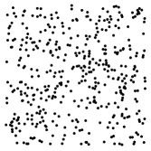
Recall that a homogeneous Poisson process is a model for complete spatial randomness (CSR), see e.g. Møller and Waagepetersen (2004) and the simulation in the first panel of Figure 3. Consider APFs $A_{0},A_{1},\ldots,A_{r}$ corresponding to independent point processes ${\bf X}_{0},{\bf X}_{1},\ldots,{\bf X}_{r}$ defined on a unit square and where ${\bf X}_{i}$ for $i>0$ is CSR with a given intensity $\rho$ (the mean number of points). Suppose ${\bf X}_{0}$ is claimed to be CSR with intensity $\rho$, however, the model for ${\bf X}_{0}$ is given by one of the following four point process models, which we refer to as the true model:

1. CSR; hence the true model agrees with the claimed model.

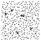
2. A Baddeley-Silverman cell process; this has the same second-order moment properties as under CSR, see Baddeley and Silverman (1984). Though from a mathematical point of view, it is a cluster process, simulated realisations will exhibit both aggregation and regularity at different scales, see the second panel of Figure 3.

3. A Matérn cluster process; this is a model for clustering where each cluster is a homogenous Poisson process within a disc and the centers of the discs are not observed and constitute a stationary Poisson process, see Matérn (1986),
   Møller and Waagepetersen (2004), and the third panel of Figure 3.

4. A most repulsive Bessel-type determinantal point process (DPP); this is a model for regularity, see Lavancier et al. (2015), Biscio and Lavancier (2016), and the fourth panel of Figure 3.

We let $\rho=100$ or $400$. This specifies completely the models in (a) and (d), whereas the remaining parameters in the cases (b)-(c) are defined to be the same as those used in Robins and Turner (2016). In all cases of Figure 3, $\rho=400$. Finally, following the recommendation in Myllymäki et al. (2016), we let $r=2499$.

Figure 3: Simulated point patterns for a homogeneous Poisson process (first panel), a Baddeley-Silverman cell process (second panel), a Matérn cluster process (third panel), and a most repulsive Bessel-type DPP (fourth panel).

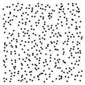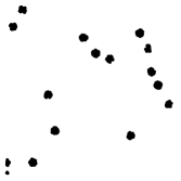
For each value of $\rho=100$ or $400$, we simulate each point process in (a)-(d) with the R-package spatstat. Then, for each dimension $k=0$ or $1$, we compute the extreme rank envelopes and extreme rank envelope tests with the R-package spptest. We repeat all this $500$ times. Table 1 shows for each case (a)-(d) the percentage of rejection of the hypothesis that ${\bf X}_{0}$ is a homogeneous Poisson process with known intensity $\rho$. In case of CSR, the type one error of the test is small except when $k=0$ and $\rho=100$. As expected in case of (b)-(d), the power of the test is increased when $\rho$ is increased. For both the Baddeley-Silverman process and the DPP, when $k=0$ and/or $\rho=400$, the power is high and even 100% in two cases. For the Matérn cluster process, the power is 100% when both $\rho=100$ and 400; this is also the case when instead the radius of a cluster becomes 10 times larger and hence it is not so easy to distinguish the clusters as in the third panel of Figure 3. When we combine the extreme rank envelopes for $\mathrm{APF}_{0}$ and $\mathrm{APF}_{1}$, the results are better or close to the best results obtained when considering only one extreme rank envelope.

	CSR		DPP		Matérn cluster		Baddeley-Silverman
	$\rho=100$	$\rho=400$	$\rho=100$	$\rho=400$	$\rho=100$	$\rho=400$	$\rho=100$	$\rho=400$
$\mathrm{APF}_{0}$	3.6	4	77.4	100	100	100	45.6	99.6
$\mathrm{APF}_{1}$	3.8	4.6	28.2	57.8	100	100	65.8	100
$\mathrm{APF}_{0}$, $\mathrm{APF}_{1}$	4.8	3.6	82.4	100	100	100	60.8	100

Table 1: Percentage of point patterns for which the $95\%$-extreme rank envelope test rejects the hypothesis of CSR (a homogeneous Poisson process on the unit square with intensity $\rho=100$ or $\rho=400$) when the true model is either CSR or one of three alternative point process models.

Figure 4 illustrates for one of the $500$ repetitions and for each dimension $k=0$ and $k=1$ the deviation of $\mathrm{APF}_{k}$ from the extreme rank envelope obtained when the true model is not CSR. For each of the three non-CSR models, $\mathrm{APF}_{k}$ is outside the extreme rank envelope, in particular when $k=0$ and both the meanage and lifetime are small, cf. the middle panel. This means that small lifetimes are not noise but of particular importance, cf. the discussion in Section 1.2. Using an obvious notation, for small $m$, we may expect that $\mathrm{APF}^{\mathrm{DPP}}_{0}(m)<\mathrm{APF}^{\mathrm{CSR}}_{0}(m)<\mathrm{APF}^{\mathrm{MC}}_{0}(m)$ which is in agreement with the middle panel. For large $m$, we may expect that $\mathrm{APF}^{\mathrm{DPP}}_{0}(m)>\mathrm{APF}^{\mathrm{CSR}}_{0}(m)$ and $\mathrm{APF}^{\mathrm{CSR}}_{0}(m)>\mathrm{APF}^{\mathrm{MC}}_{0}(m)$, but only the last relation is detected by the extreme rank envelope in the left panel. Similarly, we may expect $\mathrm{APF}^{\mathrm{MC}}_{1}(m)>\mathrm{APF}^{\mathrm{CSR}}_{1}(m)$ for small $m$, whereas $\mathrm{APF}^{\mathrm{MC}}_{1}(m)<\mathrm{APF}^{\mathrm{CSR}}_{1}(m)$ for large $m$, and both cases are detected in the right panel. Note that for the Baddeley-Silverman cell process and $k=0,1$, $\mathrm{APF}^{\mathrm{BS}}_{k}$ has a rather similar behaviour as $\mathrm{APF}^{\mathrm{DPP}}_{k}$, i.e. like a regular point process and probably because clustering is a rare phenomena.

Figure 4: $95\%$-extreme rank envelope for $\mathrm{APF}_{i}$ when $i=0$ (left panel and the enlargement shown in the middle panel) or $i=1$ (right panel) together with the curves for the three non-CSR models (Baddeley-Silverman cell process, Matérn cluster process, and Bessel-type DPP). The envelope is obtained from $2499$ realisations of a CSR model on the unit square and with intensity $100$.

A similar simulation study is discussed in Robins and Turner (2016) for the models in (a)-(c), but notice that they fix the number of points to be $100$ and they use a testing procedure based on the persistent homology rank function, which in contrast to our one-dimensional APF is a two-dimensional function and is not summarizing all the topological features represented in a persistent diagram. Robins and Turner (2016) show that a test for CSR based on the persistent homology rank function is useful as compared to various tests implemented in spatstat and which only concern first and second-order moment properties. Their method is in particular useful, when the true model is a Baddeley-Silverman cell process with the same first and second-order moment properties as under CSR. Comparing Figure 4 in Robins and Turner (2016) with the results in Table 1 when the true model is a Baddeley-Silverman cell process and $\rho=100$, the extreme rank envelope test seems less powerful than the test they suggest. On the other hand, Robins and Turner (2016) observe that the latter test performs poorly when the true model is a Strauss process (a model for inhibition) or a Matérn cluster process; as noticed for the Matérn cluster process, we obtain a perfect power when using the extreme rang envelope test.

4 A single sample of accumulated persistence functions

4.1 Functional boxplot

This section discusses the use of a functional boxplot (Sun and Genton, 2011) for a sample $A_{1},\ldots,A_{r}$ of $\mathrm{APF}_{k}$s those joint distribution is exchangeable. The plot provides a representation of the variation of the curves given by $A_{1},\ldots,A_{r}$ around the most central curve, and it can be used for outlier detection, i.e. detection of curves that are too extreme with respect to the others in the sample. This is illustrated in Example 2 for the brain artery trees dataset and in Appendix B and its accompanying Example 6 concerning a simulation study.

The functional boxplot is based on an ordering of the $\mathrm{APF}_{k}$s obtained using a so-called depth function. For specificity we make the standard choice called the modified band depth function (MBD), cf. López-Pintado and Romo (2009) and Sun and Genton (2011): For a user-specified parameter $T>0$ and $h,i,j=1,\ldots,r$ with $i<j$, define

$$B_{h,i,j}=\left\{m\in[0,T]:\ \min\left\{A_{i}\left(m\right),A_{j}\left(m\right)\right\}\leq A_{h}(m)\leq\max\left\{A_{i}\left(m\right),A_{j}\left(m\right)\right\}\right\},$$

and denote the Lebesgue measure on $[0,T]$ by $\left|\cdot\right|$. Then the MBD of $A_{h}$ with respect to $A_{1},\ldots,A_{r}$ is

$$\mathrm{MBD}_{r}(A_{h})=\frac{2}{r(r-1)}\sum_{1\leq i<j\leq r}\left|B_{h,i,j}\right|.$$ (5)

This is the average proportion of $A_{h}$ on $[0,T]$ between all possible pairs of $A_{1},\ldots,A_{r}$. Thus, the larger the value of the MBD of a curve is, the more central or deeper it is in the sample. We call the region delimited by the $50\%$ most central curves the central envelope. It is often assumed that a curve outside the central envelope inflated by $1.5$ times the range of the central envelope is an outlier or abnormal curve — this is just a generalisation of a similar criterion for the boxplot of a sample of real numbers — and the range may be changed if it is more suitable for the application at hand, see the discussion in Sun and Genton (2011) and Example 2 below.

Example 2 (brain artery trees).

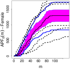
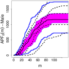
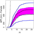
For the brain artery trees dataset (Section 2.2), Figure 5 shows the functional boxplots of $\text{APF}_{k}$s for females (first and third panels) respective males (second and fourth panels) when $k=0$ (first and second panels) and $k=1$ (third and fourth panels): The most central curve is plotted in black, the central envelope in purple, and the upper and lower bounds obtained from all the curves except the outliers in dark blue. Comparing the two left panels (concerned with connected components), the shape of the central envelope is clearly different for females and males, in particular on the interval $[40,60]$, and the upper and lower bounds of the non-outlier are closer to the central region for females, in particular on the interval $[0,50]$. For the two right panels (concerned with loops), the main difference is observed on the interval $[15,25]$ where the central envelope is larger for females than for males.

Figure 5: Functional boxplots of APFs for females and males obtained from the brain artery trees dataset: $\mathrm{APF}^{F}_{0}$ (first panel), $\mathrm{APF}^{M}_{0}$ (second panel), $\mathrm{APF}^{F}_{1}$ (third panel), $\mathrm{APF}^{M}_{1}$ (fourth panel). The dashed lines show the outliers detected by the 1.5 criterion.

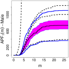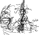
The dashed lines in Figure 5 show the APFs detected as outliers by the 1.5 criterion, that is $6$ $\mathrm{APF}^{F}_{0}$s (first panel), $3$ $\mathrm{APF}^{F}_{1}$s (third panel), $6$ $\mathrm{APF}^{M}_{0}$s (second panel), and $4$ $\mathrm{APF}^{M}_{1}$s (fourth panel). For the females, only for one point pattern both $\mathrm{APF}^{F}_{0}$ and $\mathrm{APF}^{F}_{1}$ are outliers, where $\mathrm{APF}^{F}_{1}$ is the steep dashed line in the bottom-left panel; and for the males, only for two point patterns both $\mathrm{APF}^{M}_{0}$ and $\mathrm{APF}^{M}_{1}$ are outliers, where in one case $\mathrm{APF}^{M}_{1}$ is the steep dashed line in the bottom-right panel. For this case, Figure 6 reveals an obvious issue: A large part on the right of the corresponding tree is missing!

Examples 3 and 4 discuss to what extent our analysis of the brain artery trees will be sensitive to whether we include or exclude the detected outliers.

Figure 6: Brain artery tree of a male subject with $\mathrm{APF}^{M}_{0}$ and $\mathrm{APF}^{M}_{1}$ detected as outliers by the 1.5 criterion.

4.2 Confidence region for the mean function

This section considers an asymptotic confidence region for the mean function of a sample $A_{1},\ldots,A_{r}$ of IID $\mathrm{APF}_{k}$s. We assume that $D_{1},\ldots,D_{r}$ are the underlying IID $\mathrm{RRPD}_{k}$s for the sample so that with probability one, there exists an upper bound $T<\infty$ on the death times and there exists an upper bound $n_{\mathrm{max}}<\infty$ on the number of $k$-dimensional topological features. Note that the state space for such $\mathrm{RRPD}_{k}$s is

$$\mathcal{D}_{k,T,n_{\mathrm{max}}}=\{\{(m_{1},l_{1},c_{1}),\ldots,(m_{n},l_{n},c_{n})\}:\sum_{i=1}^{n}c_{i}\leq n_{\mathrm{max}},\,m_{i}+l_{i}/2\leq T,\,i=1,\ldots,n\}$$

and only the existence and not the actual values of $n_{\mathrm{max}}$ and $T$ play a role when applying our method below. For example, in the settings (i)-(ii) of Section 2.1 it suffices to assume that $\mathbf{X}$ is included in a bounded region of $\mathbb{R}^{2}$ and that the number of points $N$ is bounded by a constant; this follows from the two versions of the Nerve Theorem presented in Fasy et al. (2014) and Edelsbrunner and Harer (2010), respectively.

We adapt an empirical bootstrap procedure (see e.g. van der Vaart and Wellner (1996)) which in Chazal et al. (2013) is used for a confidence region for the mean of the dominant function of the persistent landscape and which in our case works as follows. For $0\leq m\leq T$, the mean function is given by $\mu(m)=\mathrm{E}\left\{A_{1}(m)\right\}$ and estimated by the empirical mean function $\overline{A}_{r}(m)=\frac{1}{r}\sum_{i=1}^{r}A_{i}(m)$. Let $A^{*}_{1},\ldots,A^{*}_{r}$ be independent uniform draws with replacement from the set $\{A_{1},\ldots,A_{r}\}$ and set $\overline{A^{*}_{r}}=\frac{1}{r}\sum_{i=1}^{r}A^{*}_{i}$ and $\theta^{*}=\sup_{m\in[0,T]}\sqrt{r}\left|\overline{A_{r}}(m)-\overline{A^{*}_{r}}(m)\right|$. For a given integer $B>0$, independently repeat this procedure $B$ times to obtain $\theta_{1}^{*},\ldots,\theta_{B}^{*}$. Then, for $0<\alpha<1$, the $100(1-\alpha)\%$-quantile in the distribution of $\theta^{*}$ is estimated by

$$\hat{q}^{B}_{\alpha}=\inf\{q\geq 0:\,\frac{1}{B}\sum_{i=1}^{B}1(\theta_{i}^{*}>q)\leq\alpha\}.$$

The following theorem is verified in Appendix F.

Theorem 4.1.

Let the situation be as described above. For large values of $r$ and $B$, the functions $\overline{A_{r}}\pm\hat{q}^{B}_{\alpha}/\sqrt{r}$ provide the bounds for an asymptotic conservative $100(1-\alpha)\%$-confidence region for the mean APF, that is

$$\lim_{r\rightarrow\infty}\lim_{B\rightarrow\infty}\mathrm{P}\left(\mu(m)\in[\overline{A_{r}}(m)-\hat{q}_{\alpha}^{B}/\sqrt{r},\overline{A_{r}}(m)+\hat{q}_{\alpha}^{B}/\sqrt{r}]\mbox{ for all }m\in[0,T]\right)\geq 1-\alpha.$$

Example 3 (brain artery trees).

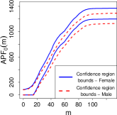
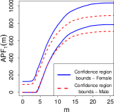
The brain artery trees are all contained in a bounded region and presented by a bounded number of points, so it is obvious that $T$ and $n_{\mathrm{max}}$ exist for $k=0,1$. To establish confidence regions for the mean of the $\mathrm{APF}^{M}_{k}$s respective $\mathrm{APF}^{F}_{k}$s, we apply the bootstrap procedure with $B=1000$. The result is shown in Figure 7 when all 95 trees are considered: In the left panel, $k=0$ and approximatively half of each confidence region overlap with the other confidence region; it is not clear if there is a difference between genders. In the right panel, $k=1$ and the difference is more pronounced, in particular on the interval $[15,25]$. Similar results and conclusions are obtained if we exclude the APFs detected as outliers in Example 2. Of course we should supply with a statistical test to assess the gender effect and such a test is established in Section 5 and applied in Example 4.

Appendix C provides the additional Example 7 for a simulated dataset along with a discussion on the geometrical interpretation of the confidence region obtained.

Figure 7: Bootstrap confidence regions for the mean $\mathrm{APF}^{M}_{k}$ and the mean $\mathrm{APF}^{F}_{k}$ when $k=0$ (left panel) and $k=1$ (right panel).

5 Two samples of accumulated persistence functions

This section concerns a two-sample test for comparison of two samples of APFs. Appendix E presents both a clustering method (Appendix E.1, including Example 9) and a unsupervised classification method (Appendix E.2, including Example 10) for two or more samples.

Consider two samples of independent $\mathrm{RRPD}_{k}$s $D_{1},\ldots,D_{r_{1}}$ and $E_{1},\ldots,E_{r_{2}}$, where each $D_{i}$ ($i=1,\ldots,r_{1}$) has distribution $\mathrm{P}_{D}$ and each $E_{j}$ has distribution $\mathrm{P}_{E}$ ($j=1,\ldots,r_{2}$), and suppose we want to test the null hypothesis $\mathcal{H}_{0}$: $\mathrm{P}_{D}=\mathrm{P}_{E}=\mathrm{P}$. Here, the common distribution $\mathrm{P}$ is unknown and as in Section 4.2 we assume it is concentrated on $\mathcal{D}_{k,T,n_{\mathrm{max}}}$ for some integer $n_{\mathrm{max}}>0$ and number $T>0$. Below, we adapt a two-sample test statistic studied in Præstgaard (1995) and van der Vaart and Wellner (1996).

Let $r=r_{1}+r_{2}$. Let $A_{1},\ldots,A_{r}$ be the $\mathrm{APF}_{k}$ corresponding to $(D_{1},\ldots,D_{r_{1}},E_{1},\ldots,E_{r_{2}})$, and denote by $\overline{A_{r_{1}}}$ and $\overline{A_{r_{2}}}$ the empirical means of $A_{1},\ldots,A_{r_{1}}$ and $A_{r_{1}+1},\ldots,A_{r_{1}+r_{2}}$, respectively. Let $I=[T_{1},T_{2}]$ be a user-specified interval with $0\leq T_{1}<T_{2}\leq T$ and used for defining a two-sample test statistic by

$$KS_{r_{1},r_{2}} =\sqrt{\frac{r_{1}r_{2}}{r}}\sup_{m\in I}\left|\overline{A_{r_{1}}}(m)-\overline{A_{r_{2}}}(m)\right|,$$ (6)

where large values are critical for $\mathcal{H}_{0}$. This may be rewritten as

$$KS_{r_{1},r_{2}}=\sup_{m\in I}\left|\sqrt{\frac{r_{2}}{r}}G^{r_{1}}_{D}(m)-\sqrt{\frac{r_{1}}{r}}G^{r_{2}}_{E}(m)+\sqrt{\frac{r_{1}r_{2}}{r}}\mathrm{E}\left\{A_{D}-A_{E}\right\}(m)\right|,$$ (7)

where $G_{D}^{r_{1}}=\sqrt{r_{1}}\left(\overline{A_{r_{1}}}-\mathrm{E}\left\{A_{D}\right\}\right)$ and $G_{E}^{r_{2}}=\sqrt{r_{2}}\left(\overline{A_{r_{2}}}-\mathrm{E}\left\{A_{E}\right\}\right)$. By Lemma F.2 in Appendix F and by the independence of the samples, $G_{D}^{r_{1}}$ and $G_{E}^{r_{2}}$ converge in distribution to two independent zero-mean Gaussian processes on $I$, denoted $G_{D}$ and $G_{E}$, respectively. Assume that $r_{1}/r\rightarrow\lambda\in(0,1)$ as $r\rightarrow\infty$. Under $\mathcal{H}_{0}$, in the sense of convergence in distribution,

$$\lim_{r\rightarrow\infty}KS_{r_{1},r_{2}}=\sup_{m\in I}\left|\sqrt{1-\lambda}G_{D}(m)-\sqrt{\lambda}G_{E}(m)\right|,$$ (8)

where $\sqrt{1-\lambda}G_{D}-\sqrt{\lambda}G_{E}$ follows the same distribution as $G_{D}$. If $\mathcal{H}_{0}$ is not true and $\sup_{m\in I}\left|\mathrm{E}\left\{A_{1}-A_{r_{1}+1}\right\}(m)\right|>0$, then $KS_{r_{1},r_{2}}\rightarrow\infty$ as $r\rightarrow\infty$, see van der Vaart and Wellner (1996). Therefore, for $0<\alpha<1$ and letting $q_{\alpha}=\inf\{q:\,\mathrm{P}(\sup_{m\in I}\left|G_{D}(m)\right|>q)\leq\alpha\}$, the asymptotic test that rejects $\mathcal{H}_{0}$ if $KS_{r_{1},r_{2}}\leq q_{\alpha}$ is of level $100\alpha\%$ and of power $100\%$.

As $q_{\alpha}$ depends on the unknown distribution $\mathrm{P}$, we estimate $q_{\alpha}$ by a bootstrap method: Let $A^{*}_{1},\ldots,A^{*}_{r}$ be independent uniform draws with replacement from $\{A_{1},\ldots,A_{r}\}$. For $0\leq m\leq T$, define the empirical mean functions $\overline{A^{*}_{r_{1}}}(m)=\frac{1}{r_{1}}\sum_{i=1}^{r_{1}}A^{*}_{i}(m)$ and $\overline{A^{*}_{r_{2}}}(m)=\frac{1}{r_{2}}\sum_{i=r_{1}+1}^{r_{1}+r_{2}}A^{*}_{i}(m)$, and compute

$$\theta^{*} =\sqrt{\frac{r_{1}r_{2}}{r}}\sup_{m\in I}\left|\overline{A^{*}_{r_{1}}}(m)-\overline{A^{*}_{r_{2}}}(m)\right|.$$ (9)

For a given integer $B>0$, independently repeat this procedure $B$ times to obtain $\theta_{1}^{*},\ldots,\theta_{B}^{*}$. Then we estimate $q_{\alpha}$ by the $100(1-\alpha)\%$-quantile of the empirical distribution of $\theta_{1}^{*},\ldots,\theta_{B}^{*}$, that is

$$\hat{q}^{B}_{\alpha}=\inf\{q\geq 0:\,\frac{1}{B}\sum_{i=1}^{B}1(\theta_{i}^{*}>q)\leq\alpha\}.$$

The next theorem is a direct application of Theorem 3.7.7 in van der Vaart and Wellner (1996) noticing that the $\mathrm{APF}_{k}$s are uniformly bounded by $Tn_{\mathrm{max}}$ and they form a so-called Donsker class, see Lemma F.2 and its proof in Appendix F.

Theorem 5.1.

Let the situation be as described above. If $r\rightarrow\infty$ such that $r_{1}/r\rightarrow\lambda$ with $\lambda\in(0,1)$, then under $\mathcal{H}_{0}$

$$\lim_{r\rightarrow\infty}\lim_{B\rightarrow\infty}\mathrm{P}\left(KS_{r_{1},r_{2}}>{\hat{q}^{B}_{\alpha}}\right)=\alpha,$$

whilst if $\mathcal{H}_{0}$ is not true and $\sup_{m\in I}\left|\mathrm{E}\left\{A_{1}-A_{r_{1}+1}\right\}(m)\right|>0$, then

$$\lim_{r\rightarrow\infty}\lim_{B\rightarrow\infty}\mathrm{P}\left(KS_{r_{1},r_{2}}>{\hat{q}^{B}_{\alpha}}\right)=1.$$

Therefore, the test that rejects $\mathcal{H}_{0}$ if $KS_{r_{1},r_{2}}>\hat{q}^{B}_{\alpha}$ is of asymptotic level $100\alpha\%$ and power $100\%$. As remarked in van der Vaart and Wellner (1996), by their Theorem 3.7.2 it is possible to present a permutation two-sample test so that the critical value $\hat{q}^{B}_{\alpha}$ for the bootstrap two-sample test has the same asymptotic properties as the critical value for the permutation test.

Other two-sample test statistics than (6) can be constructed by considering other measurable functions of $\overline{A_{r_{1}}}-\overline{A_{r_{2}}}$, e.g. we may consider the two-sample test statistic

$$M_{r_{1},r_{2}} =\int_{I}\left|\overline{A_{r_{1}}}(m)-\overline{A_{r_{2}}}(m)\right|\,\mathrm{d}m.$$ (10)

Then by similar arguments as above but redefining $\theta^{*}$ in (9) by

$$\theta^{*} =\sqrt{\frac{r_{1}r_{2}}{r}}\int_{m\in I}\left|\overline{A^{*}_{r_{1}}}(m)-\overline{A^{*}_{r_{2}}}(m)\right|\,\mathrm{d}m,$$

the test that rejects $\mathcal{H}_{0}$ if $M_{r_{1},r_{2}}>\hat{q}^{B}_{\alpha}$ is of asymptotic level $100\alpha\%$ and power $100\%$.

Example 4 (brain artery trees).

To distinguish between male and female subjects of the brain artery trees dataset, we use the two-sample test statistic $KS_{r_{1},r_{2}}$ under three different settings:

1. For $k=0,1$, we let $\mathrm{PD}_{k}^{\prime}$ be the subset of $\mathrm{PD}_{k}$ corresponding to the $100$ largest lifetimes. Then $D_{1},\ldots,D_{46}$ and $E_{1},\ldots,E_{49}$ are the $\mathrm{RRPD}_{k}$s obtained from the $\mathrm{PD}_{k}^{\prime}$s associated to female and male subjects, respectively. This is the setting used in Bendich et al. (2016).

2. For $k=0,1$, we consider all lifetimes and let $D_{1},\ldots,D_{46}$ and $E_{1},\ldots,E_{49}$ be the $\mathrm{RRPD}_{k}$s associated to female and male subjects, respectively.

3. The samples are as in setting (B) except that we exclude the $\mathrm{RRPD}_{k}$s where the corresponding $\mathrm{APF}_{k}$ was detected as an outlier in Example 2. Hence, $r_{1}=40$ and $r_{2}=43$ if $k=0$, and $r_{1}=43$ and $r_{2}=45$ if $k=1$.

Bendich et al. (2016) perform a permutation test based on the mean lifetimes for the male and female subjects and conclude that gender effect is recognized when considering $\mathrm{PD}_{1}$ ($p$-value $=3\%$) but not $\mathrm{PD}_{0}$ ($p$-value $=10\%$). For comparison, under each setting (A)-(C), we perform the two-sample test for $k=0,1$, different intervals $I$, and $B=10000$. In each case, we estimate the $p$-value, i.e. the smallest $\alpha$ such that the two-sample test with significance level $100\alpha\%$ does not reject $\mathcal{H}_{0}$, by $\hat{p}=\frac{1}{B}\sum_{i=1}^{B}1(\theta_{i}^{*}>KS_{r_{1},r_{2}})$. Table 2 shows the results. Under each setting (A)-(C), using $\mathrm{APF}_{0}$ we have a smaller $p$-value than in Bendich et al. (2016) if $I=[0,137]$ and an even larger $p$-value if $I=[0,60]$; and for $k=1$ under setting (B), our $p$-value is about seven times larger than the $p$-value in Bendich et al. (2016) if $I=[0,25]$, and else it is similar or smaller. For $k=1$ and $I=[0,25]$, the large difference between our $p$-values under settings (B) and (C) indicates that the presence of outliers violates the result of Theorem 5.1 and care should hence be taken. In our opinion we can better trust the results without outliers, where in contrast to Bendich et al. (2016) we see a clear gender effect when considering the connected components. Notice also that in agreement with the discussion of Figure 5 in Example 2, for each setting A, B, and C and each dimension $k=0,1$, the $p$-values in Table 2 are smallest when considering the smaller interval $I=[0,60]$ or $I=[15,25]$.

Appendix D provides an additional Example 8 illustrating the use of two-sample test in a simulation study.

	$\mathrm{APF}_{0}$		$\mathrm{APF}_{1}$
	$I=[0,137]$	$I=[0,60]$	$I=[0,25]$	$I=[15,25]$
Setting (A)	5.26	3.26	3.18	2.72
Setting (B)	7.67	3.64	20.06	1.83
Setting (C)	4.55	2.61	0.92	0.85

Table 2: Estimated $p$-values given in percentage of the two-sample test based on $KS_{r_{1},r_{2}}$ used with $\mathrm{APF}_{0}$ and $\mathrm{APF}_{1}$ on different intervals $I$ to distinguish between male and female subjects under settings (A), (B), and (C) described in Example 4.

Acknowledgements

Supported by The Danish Council for Independent Research | Natural Sciences, grant 7014-00074B, "Statistics for point processes in space and beyond", and by the "Centre for Stochastic Geometry and Advanced Bioimaging", funded by grant 8721 from the Villum Foundation. Helpful discussions with Lisbeth Fajstrup on persistence homology is acknowledged. In connection to the brain artery trees dataset we thank James Stephen Marron and Sean Skwerer for helpful discussions and the CASILab at The University of North Carolina at Chapel Hill for providing the data distributed by the MIDAS Data Server at Kitware, Inc. We are grateful to the editors and the referees for useful comments.

Appendix

Appendix A-F contain complements and additional examples to Sections 3-5. Our setting and notation are as follows. All the examples are based on a simulated point pattern $\{x_{1},\ldots,x_{N}\}\subset\mathbb{R}^{2}$ as described in Section 2.1, with $x_{1},\ldots,x_{N}$ being IID points where $N$ is a fixed positive integer. As in Section 1.1.1, our setting corresponds to applications typically considered in TDA where the aim is to obtain topological information about a compact set $C\subset\mathbb{R}^{2}$ which is unobserved and where possibly noise appears: For specificity, we let $x_{i}=y_{i}+\epsilon_{i}$, $i=1,\ldots,N$, where $y_{1},\ldots,y_{N}$ are IID points with support $C$, the noise $\epsilon_{1},\ldots,\epsilon_{N}$ are IID and independent of $y_{1},\ldots,y_{N}$, and $\epsilon_{i}$ follows the restriction to the square $[-10\sigma,10\sigma]^{2}$ of a bivariate zero-mean normal distribution with IID coordinates and standard deviation $\sigma\geq 0$ (if $\sigma=0$ there is no noise). We denote this distribution for $\epsilon_{i}$ by $N_{2}(\sigma)$ (the restriction to $[-10\sigma,10\sigma]^{2}$ is only imposed for technical reasons and is not of practical importance). We let $C_{t}$ be the union of closed discs of radii $t$ and centred at $x_{1},\ldots,x_{N}$, and we study how the topological features of $C_{t}$ changes as $t\geq 0$ grows. For this we use the Delaunay-complex mentioned in Section 1.1.1. Finally, we denote by $\mathcal{C}((a,b),r)$ the circle with center $(a,b)$ and radius $r$.

Appendix A Transforming confidence regions for persistence diagrams used for separating topological signal from noise

As noted in Section 3 there exists several constructions and results on confidence sets for persistence diagrams when the aim is to separate topological signal from noise, see Fasy et al. (2014), Chazal et al. (2014), and the references therein. We avoid presenting the technical description of these constructions and results, which depend on different choices of complexes (or more precisely so-called filtrations). For specificity, in this appendix we just consider the Delaunay-complex and discuss the transformation of such a confidence region into one for an accumulate persistence function.

We use the following notation. As in the aforementioned references, consider the persistence diagram $\mathrm{PD}_{k}$ for an unobserved compact manifold $C\subset\mathbb{R}^{2}$ and obtained as in Section 1.1.1 by considering the persistence as $t\geq 0$ grows of $k$-dimensional topological features of the set consisting of all points in $\mathbb{R}^{2}$ within distance $t$ from $C$. Note that $\mathrm{PD}_{k}$ is considered as being non-random and unknown; of course in our simulation study presented in Example 5 below we only pretend that $\mathrm{PD}_{k}$ is unknown. Let $\widehat{\mathrm{PD}}_{k,N}$ be the random persistence diagram obtained as in Section 1.1.1 from IID points $x_{1},\ldots,x_{N}$ with support $C$. Let $\mathcal{N}=\{(b,d):\,b\leq d,\,l\leq 2c_{N}\}$ be the set of points at distance $\sqrt{2}c_{N}$ of the diagonal in the persistence diagram. Let $S(b,d)=\{(x,y):\,|x-b|\leq c_{N},\,|y-d|\leq c_{N}\}$ be the square with center $(b,d)$, sides parallel to the $b$- and $d$-axes, and of side length $2c_{N}$. Finally, let $\alpha\in(0,1)$.

Fasy et al. (2014) and Chazal et al. (2014) suggest various ways of constructing a bound $c_{N}>0$ so that an asymptotic conservative $100(1-\alpha)\%$-confidence region for $\mathrm{PD}_{k}$ with respect to the bottleneck distance $W_{\infty}$ is given by

$$\liminf_{N\rightarrow\infty}\mathrm{P}\left(W_{\infty}(\mathrm{PD}_{k},\widehat{\mathrm{PD}}_{k,N})\leq c_{N}\right)\geq 1-\alpha$$ (11)

where $W_{\infty}$ is the bottleneck distance defined in Section 1.3. The confidence region given by (11) consists of those persistence diagrams $\mathrm{PD}_{k}$ which have exactly one point in each square $S(b_{i},d_{i})$, with $(b_{i},d_{i})$ a point of $\widehat{\mathrm{PD}}_{k,N}$, and have an arbitrary number of points in the set $\mathcal{N}$. Fasy et al. (2014) consider the points of $\widehat{\mathrm{PD}}_{k,N}$ falling in $\mathcal{N}$ as noise and the remaining points as representing a significant topological feature of $C$.

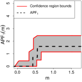
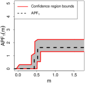
Using (11) an asymptotic conservative $100(1-\alpha)\%$-confidence region for the $\mathrm{APF}_{k}$ corresponding to $\mathrm{PD}_{k}$ is immediately obtained. This region will be bounded by two functions $\widehat{A}^{\mathrm{min}}_{k,N}$ and $\widehat{A}^{\mathrm{max}}_{k,N}$ specified by $\widehat{\mathrm{PD}}_{k,N}$ and $c_{N}$. Due to the accumulating nature of $\mathrm{APF}_{k}$, the span between the bounds is an increasing function of the meanage. When using the Delaunay-complex, Chazal et al. (2014) show that the span decreases as $N$ increases; this is illustrated in Example 5 below.

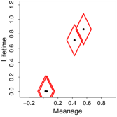
Example 5 (simulation study).

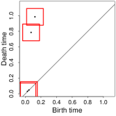
Let $C=\mathcal{C}((-1.5,0),1)\cup\mathcal{C}((1.5,0),0.8)$ and suppose each point $x_{i}$ is uniformly distributed on $C$. Figure 8 shows $C$ and an example of a simulated point pattern with $N=300$ points. We use the bootstrap method implemented in the R-package TDA and presented in Chazal et al. (2014) to compute the $95\%$-confidence region for $\mathrm{PD}_{1}$ when $N=300$, see the top-left panel of Figure 9, where the two squares above the diagonal correspond to the two loops in $C$ and the other squares correspond to topological noise. Thereby $95\%$-confidence regions for $\mathrm{RRPD}_{1}$ (top-right panel) and $\mathrm{APF}_{1}$ (bottom-left panel) are obtained. The confidence region for $\mathrm{APF}_{1}$ decreases as $N$ increases as demonstrated in the bottom panels where $N$ is increased from 300 to 500. As noticed in Section 1.3, we must be careful when using results based on the bottleneck metric, because small values of the bottleneck metric does not correspond to closeness of the two corresponding APFs: Although close persistence diagram with respect to the bottleneck distance imply that the two corresponding APFs are close with respect to the $L^{q}$-norm ($1\leq q\leq\infty$), the converse is not true. Hence, it is possible that an APF is in the confidence region plotted in Figure 9 but that the corresponding persistence diagram is very different from the truth.

Figure 8: The set $C$ in Example 5 (left panel) and a simulated point pattern of $N=300$ independent and uniformly distributed points on $C$ (right panel).

Figure 9: $95\%$-confidence regions obtained by the bootstrap method for $\mathrm{PD}_{1}$ (top-left panel) and its corresponding $\mathrm{RRPD}_{1}$ (top-right panel) when $C$ and $x_{1},\ldots,x_{300}$ are as in Figure 8. The bottom-left panel shows the corresponding $95\%$-confidence region for $\mathrm{APF}_{1}$. The bottom-right panel shows the $95\%$-confidence region for $\mathrm{APF}_{1}$ when a larger point cloud with $300$ points is used.

Appendix B Additional example related to Section 4.1 "Functional boxplot"

The functional boxplot described in Section 4.1 can be used as an exploratory tool for the curves given by a sample of $\mathrm{APF}_{k}$s. It provides a representation of the most central curve and the variation around this. It can also be used for outliers detection as illustrated in the following example.

Example 6 (simulation study).

We consider a sample of $65$ independent $\mathrm{APF}_{k}$s, where the joint distribution of the first $50$ $\mathrm{APF}_{k}$s is exchangeable, whereas the last $15$ play the role of outliers. We suppose each $\mathrm{APF}_{k}$ corresponds to a point process of $100$ IID points, where each point $x_{i}$ follows one of the following distributions $\mathrm{P}_{1},\ldots,\mathrm{P}_{4}$.

• $\mathrm{P}_{1}$ (unit circle): $x_{i}$ is a uniform point on $\mathcal{C}((0,0),1)$ perturbed by $N_{2}\left(0.1\right)$-noise.

• $\mathrm{P}_{2}$ (Gaussian mixture): Let $y_{i}$ follow $N_{2}\left(0.2\right)$, then $x_{i}=y_{i}$ with probability $0.5$, and $x_{i}=y_{i}+(1.5,0.5)$ otherwise.

• $\mathrm{P}_{3}$ (two circles): $x_{i}$ is a uniform point on $\mathcal{C}((-1,-1),1)\cup\mathcal{C}((1,1),0.5)$ perturbed by $N_{2}\left((0,0),0.1\right)$-noise.

• $\mathrm{P}_{4}$ (circle of radius $0.7$): $x_{i}$ is a uniform point on $\mathcal{C}((0,0),0.7)$ perturbed by $N_{2}\left(0.1\right)$-noise.

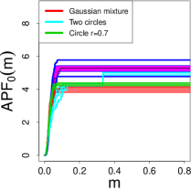
We let the first $50$ point processes be obtained from $\mathrm{P}_{1}$ (the distribution for non-outliers), the next $5$ from $\mathrm{P}_{2}$, the following $5$ from $\mathrm{P}_{3}$, and the final $5$ from $\mathrm{P}_{4}$. Figure 10 shows a simulated realization of each of the four types of point processes.

Figure 10: Simulated realizations of the four types of point processes, each consisting of 100 IID points with distribution either $\mathrm{P}_{1}$ (black dots), $\mathrm{P}_{2}$ (blue crosses), $\mathrm{P}_{3}$ (red triangles), or $\mathrm{P}_{4}$ (rotated green crosses).

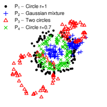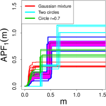
Figure 11 shows the functional boxplots when considering $\mathrm{APF}_{0}$ (left panel) and $\mathrm{APF}_{1}$ (right panel). The curves detected as outliers and corresponding to the distributions $\mathrm{P}_{2},\mathrm{P}_{3}$, and $\mathrm{P}_{4}$ are plotted in red, blue, and green, respectively. In both panels the outliers detected by the 1.5 criterion agree with the true outliers.

In the left panel, each curve has an accumulation of small jumps between $m=0$ and $m\approx 0.1$, corresponding to the moments where the points associated to each circle are connected by the growing discs in the sequence $\{C_{t}\}_{t\geq 0}$. The curves corresponding to realisations of $P_{3}$ have a jump at $m\approx 0.38$ which corresponds to the moment where the points associated to the two circles used when defining $P_{3}$ are connected by the growing discs in the sequence $\{C_{t}\}_{t\geq 0}$. The points following the distribution $P_{4}$ are generally closer to each other than the ones following the distribution $P_{1}$ as the radius of the underlying circle is smaller. This corresponds to more but smaller jumps in $\mathrm{APF}_{0}$ for small meanages, and hence the curves of $\mathrm{APF}_{0}$ are lower when they correspond to realisations of $P_{1}$ than to realisations of $P_{4}$; and as expected, for large meanages, the curves of $\mathrm{APF}_{0}$ are larger when they correspond to realisations of $P_{1}$ than to realisations of $P_{4}$. Note that if we redefine $P_{4}$ so that the $N_{2}\left(0.1\right)$-noise is replaced by $N_{2}\left(0.07\right)$-noise, then the curves would be the same up to rescaling.

In the right panel, we observe clear jumps in all $\mathrm{APF}_{1}$s obtained from $P_{1}$, $P_{3}$, and $P_{4}$. These jumps correspond to the first time that the loops of the circles in $P_{1}$, $P_{3}$, and $P_{4}$ are covered by the union of growing discs in the sequence $\{C_{t}\}_{t\geq 0}$. Once again, if we have used $N_{2}\left(0.07\right)$-noise in place of $N_{2}\left(0.1\right)$-noise in the definition of $P_{4}$, the curves would be the same up to rescaling.

If we repeat everything but with the distribution $P_{4}$ redefined so that $\mathcal{C}((0,0),0.7)$ is replaced by $\mathcal{C}((0,0),0.8)$, then the support of $P_{4}$ is closer to that of $P_{1}$ and it becomes harder in the case of $\mathrm{APF}_{0}$ to detect the outliers with distribution $P_{4}$ (we omit the corresponding plot); thus further simulations for determining a stronger criterion would be needed.

Figure 11: Functional boxplots of $65$ APFs based on the topological features of dimension $0$ (left panel) and $1$ (right panel). In each panel, 50, 5, 5, and 5 APFs are obtained from the Delaunay-complex of $100$ IID points from the distribution $\mathrm{P}_{1}$, $\mathrm{P}_{2}$, $\mathrm{P}_{3}$, and $\mathrm{P}_{4}$, respectively. The APFs detected as outliers are plotted in red, blue, and green in the case of $\mathrm{P}_{2}$, $\mathrm{P}_{3}$, and $\mathrm{P}_{4}$, respectively.

Appendix C Additional example related to Section 4.2 "Confidence region for the mean function"

This appendix provides yet an example to illustrate the bootstrap method in Section 4.2 for obtaining a confidence region for the mean function of a sample of IID $\mathrm{APF}_{k}$s.

Example 7 (simulation study).

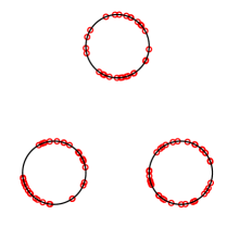
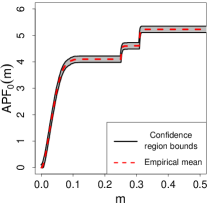
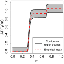
Consider 50 IID copies of a point process consisting of 100 independent and uniformly distributed points on the union of three circles with radius $0.25$ and centred at $(-1,-1)$, $(0,1)$, and $(1,-1)$, respectively (these circles were also considered in the example of Section 1.1.1). A simulated realization of the point process is shown in the left panel of Figure 12, and the next two panels show simulated confidence regions for $\mathrm{APF}_{0}$ and $\mathrm{APF}_{1}$, respectively, when the bootstrap procedure with $B=1000$ is used. In the middle panel, between $m=0$ and $m=0.2$, there is an accumulation of small jumps corresponding to the moment when each circle is covered by the union of growing discs from the sequence $\{C_{t}\}_{t\geq 0}$; we interpret these small jumps as topological noise. The jump at $m\approx 0.25$ corresponds to the moment when the circles centred at $(-1,-1)$ and $(1,-1)$ are connected by the growing discs, and the jump at $m\approx 0.3$ to when all three circles are connected by the growing discs. In the right panel, at $m\approx 0.3$ there is an accumulation of small jumps corresponding to the moment when the three circles are connected by the growing discs and they form a loop at $m=0.25$ in Figure 1. The disappearance of this loop at $m=0.69$ in Figure 1 corresponds to the jump at $m\approx 0.7$ in Figure 12.

Figure 12: A simulation of 100 independent and uniformly distributed points on the union of three circles (dashed lines) with the same radius $r=0.5$ and centred at $(-1,-1)$, $(0,1)$, and $(1,-1)$ (left panel). The $95\%$-confidence regions for the mean $\mathrm{APF}_{0}$ (middle panel) and the mean $\mathrm{APF}_{1}$ (right panel) are based on 50 IID simulations.

Appendix D Additional example to Section 5 "Two samples of accumulated persistence functions"

Section 5 considered two samples of independent $\mathrm{RRPD}_{k}$s $D_{1},\ldots,D_{r_{1}}$ and $E_{1},\ldots,E_{r_{2}}$, where each $D_{i}$ ($i=1,\ldots,r_{1}$) has distribution $\mathrm{P}_{D}$ and each $E_{j}$ has distribution $\mathrm{P}_{E}$ ($j=1,\ldots,r_{2}$). Then we studied a bootstrap two-sample test to asses the null hypothesis $\mathcal{H}_{0}$: $\mathrm{P}_{D}=\mathrm{P}_{E}$, e.g. in connection to the brain artery trees. An additional example showing the performance of the test is presented below.

Example 8 (simulation study).

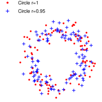
Let $\mathrm{P}_{D}$ be the distribution of a $\mathrm{RRPD}_{k}$ obtained from $100$ independent and uniformly distributed points on $\mathcal{C}((0,0),1)$ perturbed by $N_{2}\left(0.2\right)$-noise, and define $\mathrm{P}_{E}$ in a similar way but with a circle of radius $0.95$. A simulated realisation of each point process is shown in Figure 13; it seems difficult to recognize that the underlying circles are different. Let us consider the two-sample test statistics (6) and (10) with $I=[0,3]$, $r_{1}=r_{2}=50$, and $\alpha=0.05$. Over $500$ simulations of the two samples of $\mathrm{RRPD}_{k}$ we obtain the following percentage of rejection: For $M_{r_{1},r_{2}}$, $5.2\%$ if $k=0$, and $24.2\%$ if $k=1$. For $KS_{r_{1},r_{2}}$ much better results are observed, namely $73.8\%$ if $k=0$, and $93.8\%$ if $k=1$, where this high percentage is mainly caused by the largest lifetime of a loop.

Figure 13: A simulation of $100$ independent and uniformly distributed points on the circle centred at $(0,0)$ with radius $1$ and perturbed by $N_{2}\left((0,0),0.2\right)$-noise (red dots), together with $100$ independent and uniformly distributed points on the circle centred at $(0,0)$ with radius $0.95$ and perturbed by $N_{2}\left((0,0),0.2\right)$-noise (blue crosses).

Appendix E Further methods for two or more samples of accumulated persistence functions

E.1 Clustering

Suppose $A_{1},\ldots,A_{r}$ are $\mathrm{APF}_{k}$s which we want to label into $K<r$ groups by using a method of clustering (or unsupervised classification). Such methods are studied many places in the literature for functional data, see the survey in Jacques and Preda (2014). In particular, Chazal et al. (2009), Chen et al. (2015), and Robins and Turner (2016) consider clustering in connection to $\mathrm{RRPD}_{k}$s. Whereas the $\mathrm{RRPD}_{k}$s are two-dimensional functions, it becomes easy to use clustering for the one-dimensional $\mathrm{APF}_{k}$s as illustrated in Example 9 below.

For simplicity we just consider the standard technique known as the $K$-means clustering algorithm (Hartigan and Wong (1979)). For more complicated applications than considered in Example 9 the EM-algorithm may be needed for the $K$-means clustering algorithm. As noticed by a referee, to avoid the use of the EM-algorithm we can modify (9) or (10) and thereby construct a distance/similarity matrix for different APFs which is used to perform hierarchical clustering. However, for Example 9 the results using hierarchical clustering (omitted here) were not better than with the $K$-means algorithm.

Assume that $A_{1},\ldots,A_{r}$ are pairwise different and square-integrable functions on $[0,T]$, where $T$ is a user-specified parameter. For example, if $\mathrm{RRPD}_{k}\in\mathcal{D}_{k,T,n_{\mathrm{max}}}$ (see Section 4.2), then $\mathrm{APF}_{k}\in L^{2}([0,T])$. The $K$-means clustering algorithm works as follows.

• Chose uniformly at random a subset of $K$ functions from $\{A_{1},\ldots,A_{r}\}$; call these functions centres and label them by $1,\ldots,K$.

• Assign each non-selected $\mathrm{APF}_{k}$ the label $i$ if it is closer to the centre of label $i$ than to any other centre with respect to the $L^{2}$-distance on $L^{2}([0,T])$.

• In each group, reassign the centre by the mean curve of the group (this may not be an $\mathrm{APF}_{k}$ of the sample).

• Iterate these steps until the assignment of centres does not change.

The algorithm is known to be convergent, however, it may have several drawbacks as discussed in Hartigan and Wong (1979) and Bottou and Bengio (1995).

Example 9 (simulation study).

Consider $K=3$ groups, each consisting of 50 $\mathrm{APF}_{0}$s and associated to point processes consisting of $100$ IID points, where each point $x_{i}$ follows one of the following distributions $\mathrm{P}_{1}$, $\mathrm{P}_{2}$, and $\mathrm{P}_{3}$ for groups 1, 2, and 3, respectively.

• $\mathrm{P}_{1}$ (unit circle): $x_{i}$ is a uniform point on $\mathcal{C}((0,0),1)$ perturbed by $N_{2}\left(0.1\right)$-noise.

• $\mathrm{P}_{2}$ (two circles): $x_{i}$ is a uniform point on $\mathcal{C}((-1,-1),0.5)\cup\mathcal{C}((1,1),0.5)$ perturbed by $N_{2}\left(0.1\right)$-noise.

• $\mathrm{P}_{3}$ (circle of radius 0.8): $x_{i}$ is a uniform point on $\mathcal{C}((0,0),0.8)$ perturbed by $N_{2}\left(0.1\right)$-noise.

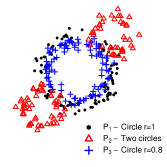
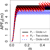
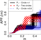
We start by simulating a realization of each of the $3\times 50=150$ point processes. The left panel of Figure 14 shows one realization of each type of point process; it seems difficult to distinguish the underlying circles for groups 1 and 3, but the three $\mathrm{APF}_{0}$s associated to these three point patterns are in fact assigned to their right groups. The right panel of Figure 14 shows the result of the $K$-means clustering algorithm. Here we are using the R-function “kmeans” for the $K$-means algorithm and it takes only a few seconds when evaluating each $A_{i}(m)$ at $2500$ equidistant values of $m$ between $0$ and $T=0.5$. As expected we see more overlap between the curves of the $\mathrm{APF}_{0}$s assigned to groups 1 and 3.

We next repeat 500 times the simulation of the 150 point processes. A clear distinction between the groups is obtained by the $K$-means algorithm applied for connected components: The percentage of wrongly assigned $\mathrm{APF}_{0}$s among the $500\times 3\times 50=75000$ $\mathrm{APF}_{0}$s has an average of $4.5\%$ and a standard deviation of $1.6\%$. The assignment error is in fact mostly caused by incorrect labelling of $\mathrm{APF}_{0}$s associated to $\mathrm{P}_{1}$ or $\mathrm{P}_{3}$. This is expected as the underlying circles used in the definitions of $P_{1}$ and $P_{3}$ are rather close, whereas the underlying set in the definition of $P_{2}$ is different with two connected components as represented by the jump at $m\approx 0.4$ in the middle panel of Figure 14.

Even better results are obtained when considering loops instead of connected components: The percentage of wrongly assigned $\mathrm{APF}_{1}$s among the $75000$ $\mathrm{APF}_{1}$s has an average of $1.6\%$ and a standard deviation of $1.0\%$. This is mainly due to the sets underlying $P_{1}$, $P_{2}$, and $P_{3}$ which have distinctive loops that results in clear distinct jumps in the $\mathrm{APF}_{1}$s as seen in the right panel of Figure 14.

Figure 14: Left panel: Simulated example of the three point processes, each consisting of $100$ IID points drawn from the distribution $P_{1}$ (black dots), $P_{2}$ (red triangles), or $P_{3}$ (blue crosses). Middle panel: The 150 $\mathrm{APF}_{0}$s obtained from the simulation of the $150$ point processes associated to $\mathrm{P}_{1}$, $\mathrm{P}_{2}$, or $\mathrm{P}_{3}$, where the colouring in black, red, or blue specifies whether the $K$-means algorithm assigns an $\mathrm{APF}_{0}$ to the group associated to $P_{1}$, $P_{2}$, or $P_{3}$. Right panel: As the middle panel but for the 150 $\mathrm{APF}_{1}$s.

E.2 Supervised classification

Suppose we want to assign an $\mathrm{APF}_{k}$ to a training set of $K$ different groups $\mathcal{G}_{1},\ldots,\mathcal{G}_{K}$, where $\mathcal{G}_{i}$ is a sample of $r_{i}$ independent $\mathrm{APF}_{k}$s $A^{i}_{1},\ldots,A^{i}_{r_{i}}$. For this purpose supervised classification methods for functional data may be adapted.

We just consider a particular method by López-Pintado et al. (2010): Suppose $\alpha\in[0,1]$ and we believe that at least $100(1-\alpha)\%$ of the $\mathrm{APF}_{k}$s in each group are IID, whereas the remaining $\mathrm{APF}_{k}$s in each group follow a different distribution and are considered as outliers (see Section 4.1). For a user-specified parameter $T>0$ and $i=1,\ldots,K$, define the $100\alpha\%$-trimmed mean $\overline{A}^{\,\alpha}_{i}$ with respect to $\mathcal{G}_{i}$ as the mean function on $[0,T]$ of the $100(1-\alpha)\%$ $\mathrm{APF}_{k}$s in $\mathcal{G}_{i}$ with the largest $\mathrm{MBD}_{r_{i}}$, see (5). Assuming $\cup_{i=1}^{K}\mathcal{G}_{i}\subset L^{2}([0,T])$, an $\mathrm{APF}_{k}$ $A\in L^{2}([0,T])$ is assigned to $\mathcal{G}_{i}$ if

$$i=\operatorname*{argmin}_{j\in\{1,\ldots,K\}}\|\overline{A}^{\,\alpha}_{j}-A\|,$$ (12)

where $\|\cdot\|$ denotes the $L^{2}$-distance. Here, the trimmed mean is used for robustness and allows a control over the curves we may like to omit because of outliers, but e.g. the median could have been used instead.

Example 10 (simulation study).

Consider the following distributions $\mathrm{P}_{1},\ldots,\mathrm{P}_{4}$ for a point $x_{i}$.

• $\mathrm{P}_{1}$ (unit circle): $x_{i}$ is a uniform point on $\mathcal{C}((0,0),1)$ which is perturbed by $N_{2}\left(0.1\right)$-noise.

• $\mathrm{P}^{\prime}_{1}$ (two circles, radii 1 and 0.5): $x_{i}$ is a uniform point on $\mathcal{C}((0,0),1)\cup\mathcal{C}((1.5,1.5),0.5)$ and perturbed by $N_{2}\left(0.1\right)$-noise.

• $\mathrm{P}_{2}$ (circle of radius 0.8): $x_{i}$ is a uniform point on $\mathcal{C}((0,0),0.8)$ which is perturbed by $N_{2}\left(0.1\right)$-noise.

• $\mathrm{P}^{\prime}_{2}$ (two circles, radii 0.8 and 0.5): $x_{i}$ is a uniform point on $\mathcal{C}((0,0),0.8)\cup\mathcal{C}((1.5,1.5),0.5)$ and perturbed by $N_{2}\left(0.1\right)$-noise.

For $k=0,1$ we consider the following simulation study: $K=2$ and $r_{1}=r_{2}=50$; $\mathcal{G}_{1}$ consists of $45$ $\mathrm{APF}_{k}$s associated to simulations of point processes consisting of $100$ IID points with distribution $\mathrm{P}_{1}$ (the non-outliers) and $5$ $\mathrm{APF}_{k}$s obtained in the same way but from $\mathrm{P}^{\prime}_{1}$ (the outliers); $\mathcal{G}_{2}$ is specified in the same way as $\mathcal{G}_{1}$ but replacing $\mathrm{P}_{1}$ and $\mathrm{P}^{\prime}_{1}$ with $\mathrm{P}_{2}$ and $\mathrm{P}^{\prime}_{2}$, respectively; and we have correctly specified that $\alpha=0.2$. Then we simulate 100 $\mathrm{APF}_{k}$s associated to $P_{1}$ and 100 $\mathrm{APF}_{k}$s associated to $P_{2}$, i.e. they are all non-outliers. Finally, we use (12) to assign each of these 200 $\mathrm{APF}_{k}$s to either $\mathcal{G}_{1}$ or $\mathcal{G}_{2}$.

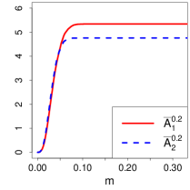
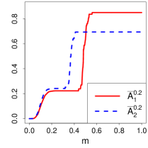
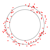
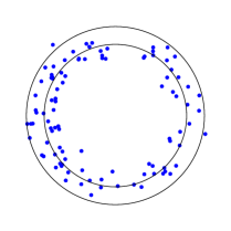
The top panels in Figure 15 show the $20\%$-trimmed means $\overline{A}^{\,0.2}_{1}$ and $\overline{A}^{\,0.2}_{2}$ when $k=0$ (left) and $k=1$ (right). The difference between the $20\%$-trimmed means is clearest when $k=1$ and so we expect that the assignment error is lower in that case. In fact wrong assignments happen mainly when the support of $\mathrm{P}_{1}$ or $\mathrm{P}_{2}$ is not well covered by the point pattern as illustrated in the bottom panels.

Figure 15: Top panels: The $20\%$-trimmed mean functions with respect to $\mathcal{G}_{1}$ and $\mathcal{G}_{2}$ when considering $\mathrm{APF}_{0}$s (left) and $\mathrm{APF}_{1}$s (right) obtained from the Delaunay-complex and based on $100$ IID points following the distribution $\mathrm{P}_{1}$ (solid curve) or $\mathrm{P}_{2}$ (dotted curve). Bottom panels: Examples of point patterns with associated $\mathrm{APF}_{0}$s assigned to the wrong group, together with the circles of radius $0.8$ and $1$.

Repeating this simulation study $500$ times, the percentage of $\mathrm{APF}_{0}$s wrongly assigned among the $500$ repetitions has a mean of $6.7\%$ and a standard deviation of $1.7\%$, whereas for the $\mathrm{APF}_{1}$s the mean is $0.24\%$ and the standard deviation is $0.43\%$. To investigate how the results depend on the radius of the smallest circle, we repeat everything but with radius $0.9$ in place of $0.8$ when defining the distributions $\mathrm{P}_{2}$ and $\mathrm{P}_{2}^{\prime}$. Then for the $\mathrm{APF}_{0}$s, the proportion of wrong assignments has a mean of $23.2\%$ and a standard deviation of $2.9\%$, and for the $\mathrm{APF}_{1}$s, a mean of $5.7\%$ and a standard deviation of $1.9\%$. Similar to Example 9, the error is lowest when $k=1$ and this is due to the largest lifetime of a loop.

Appendix F Proof of Theorem 4.1

The proof of Theorem 4.1 follows along similar lines as in Chazal et al. (2013) as soon as we have verified Lemma F.2 below. Note that the proof of Lemma F.2 is not covered by the approach in Chazal et al. (2013).

We first need to recall the following definition, where $\mathcal{B}_{T}$ denotes the topological space of bounded real valued Borel functions defined on $[0,T]$ and its topology is induced by the uniform norm.

Definition F.1.

A sequence $\left\{X_{r}\right\}_{r=1,2,\ldots}$ of random elements in $\mathcal{B}_{T}$ converges in distribution to a random element $X$ in $\mathcal{B}_{T}$ if for any bounded continuous function $f:\mathcal{B}_{T}\mapsto\mathbb{R}$, $\mathrm{E}f(X_{r})$ converges to $\mathrm{E}f(X)$ as $r\rightarrow\infty$.

Lemma F.2.

Let the situation be as in Section 4.2. As $r\rightarrow\infty$, $\sqrt{r}\left(\overline{A}_{r}-\mu\right)$ converges in distribution towards a zero-mean Gaussian process on $[0,T]$ with covariance function $c(m,m^{\prime})=\mathrm{Cov}\left(A_{1}(m),A_{1}(m^{\prime})\right)$, $m,m^{\prime}\in[0,T]$.

Proof.

We need some notation and to recall some concepts of empirical process theory. For $D\in\mathcal{D}_{T}^{k,n_{\mathrm{max}}}$, denote $A_{D}$ the $\mathrm{APF}_{k}$ of $D$. Let $\mathcal{F}=\{f_{m}:0\leq m\leq T\}$ be the class of functions $f_{m}:\mathcal{D}_{T}^{k,n_{\mathrm{max}}}\mapsto[0,\infty)$ given by $f_{m}(D)=A_{D}(m)$. To see the connection with empirical process theory, we consider

$$\mathbb{G}_{r}(f_{m})=\sqrt{r}\left(\frac{1}{r}\sum_{i=1}^{r}f_{m}(D_{i})-\mu(m)\right)$$

as an empirical process. Denote $\|\cdot\|$ the $L^{2}$ norm on $\mathcal{F}$ with respect to the distribution of $D_{1}$, i.e. $\|f_{m}(\cdot)\|^{2}=\mathrm{E}\left\{A_{D_{1}}(m)^{2}\right\}$. For $u,v\in\mathcal{F}$, the bracket $[u,v]$ is the set of all functions $f\in\mathcal{F}$ with $u\leq f\leq v$. For any $\epsilon>0$, $N_{[]}(\epsilon,\mathcal{F},\|\cdot\|)$ is the smallest integer $J\geq 1$ such that $\mathcal{F}\subset\cup_{j=1}^{J}[u_{j},v_{j}]$ for some functions $u_{1},\ldots,u_{J}$ and $v_{1},\ldots,v_{J}$ in $\mathcal{F}$ with $\|v_{j}-u_{j}\|\leq\epsilon$ for $j=1,\ldots,J$. We show below that $\int_{0}^{1}\sqrt{\log\left(N_{[]}\left(\epsilon,\mathcal{F},\|\cdot\|\right)\right)}\ \mathrm{d}\epsilon$ is finite. Then, by Theorem 19.5 in van der Vaart (2000), $\mathcal{F}$ is a so-called Donsker class which implies the convergence in distribution of $\mathbb{G}_{r}(f_{m})$ to a Gaussian process as in the statement of Lemma F.2.

For any sequence $-\infty=t_{1}<\ldots<t_{J}=\infty$ with $J\geq 2$, for $j=1,\ldots,J-1$, and for $D=\{(m_{1},l_{1},c_{1}),\ldots,(m_{n},l_{n},c_{n})\}\in\mathcal{D}_{T}^{k,n_{\mathrm{max}}}$, let $u_{j}(D)=\sum_{i=1}^{n}c_{i}l_{i}1(m_{i}\leq t_{j})$ and $v_{j}(D)=\sum_{i=1}^{n}c_{i}l_{i}1(m_{i}<t_{j+1})$ (if $n=0$, then $D$ is empty and we set $u_{j}(D)=v_{j}(D)=0$). Then, for any $m\in[0,T]$, there exists a $j=j(m)$ such that $u_{j}(D)\leq f_{m}(D)\leq v_{j}(D)$, i.e. $f_{m}(D)\in[u_{j},v_{j}]$. Consequently, $\mathcal{F}\subset\cup_{j=1}^{J-1}[u_{j},v_{j}]$.

We prove now that for any $\epsilon\in(0,1)$, the sequence $\{t_{j}\}_{1\leq j\leq J}$ can be chosen such that for $j=1,\ldots,J-1$, we have $\|v_{j}-u_{j}\|\leq\epsilon$. Write $D_{1}=\{(M_{1},L_{1},C_{1}),\ldots,(M_{N},L_{N},C_{N})\}$, where $N$ is random and should not to be confused with $N$ in Sections 2.1 and A (if $N=0$, then $D_{1}$ is empty). Let $n\in\{1,\ldots,n_{\mathrm{max}}\}$ and conditioned on $N=n$, let $I$ be uniformly selected from $\{1,\ldots,n\}$. Then

$$\mathrm{E}\left\{\left(v_{j}\left(D_{1}\right)-u_{j}\left(D_{1}\right)\right)^{2}1\left(N=n\right)\right\} =n^{2}\mathrm{E}\left\{1\left(N=n\right)\frac{1}{n}\sum_{i=1}^{n}C_{i}L_{i}1\left(M_{i}\in\left(t_{j},t_{j+1}\right)\right)\right\}^{2}$$

$$\leq T^{2}n_{\mathrm{max}}^{4}\mathrm{E}\left\{1\left(N=n\right)1\left(M_{I}\in\left(t_{j},t_{j+1}\right)\right)\right\}^{2}$$

$$\leq T^{2}n_{\mathrm{max}}^{4}\mathrm{P}\left(M_{I}\in\left(t_{j},t_{j+1}\right)|N=n\right),$$

as $n\leq n_{\mathrm{max}}$, $C_{i}\leq n_{\mathrm{max}}$, and $L_{i}\leq T$. Further,

$$\mathrm{E}\left\{\left(v_{j}\left(D_{1}\right)-u_{j}\left(D_{1}\right)\right)^{2}1\left(N=0\right)\right\} =0.$$

Hence

$$\mathrm{E}\left\{v_{j}\left(D_{1}\right)-u_{j}\left(D_{1}\right)\right\}^{2} =\sum_{n=0}^{n_{\mathrm{max}}}\mathrm{E}\left\{\left(v_{j}\left(D_{1}\right)-u_{j}\left(D_{1}\right)\right)^{2}1\left(N=n\right)\right\}$$

$$\leq T^{2}n_{\mathrm{max}}^{5}\max_{n=1,\ldots,n_{\mathrm{max}}}\mathrm{P}\left(M_{I}\in\left(t_{j},t_{j+1}\right)|N=n\right).$$ (13)

Moreover, by Lemma F.3 below, there exists a finite sequence $\{t_{n,j}\}_{1\leq j\leq J_{n}}$ such that $\mathrm{P}(M_{I}\in(t_{n,j},t_{n,j+1})|N=n)\leq\epsilon^{2}/\left(T^{2}n_{\mathrm{max}}^{5}\right)$ and $J_{n}\leq 2+T^{2}n_{\mathrm{max}}^{5}/\epsilon^{2}$. Thus, by choosing

$$\{t_{j}\}_{1\leq j\leq J}=\bigcup_{n=1,\ldots,n_{\mathrm{max}}}\{t_{n,j}\}_{1\leq j\leq J_{n}},$$

we have $J\leq 2n_{\mathrm{max}}+T^{2}n_{\mathrm{max}}^{6}/\epsilon^{2}$ and

$$\max_{n=1,\ldots,n_{\mathrm{max}}}\mathrm{P}\left(M_{I}\in\left(t_{j},t_{j+1}\right)|N=n\right)\leq\frac{\epsilon^{2}}{T^{2}n_{\mathrm{max}}^{5}}.$$

Hence by (F), $\|v_{j}-u_{j}\|\leq\epsilon$, and so by definition, $N_{[]}\left(\epsilon,\mathcal{F},\|\cdot\|\right)\leq 2n_{\mathrm{max}}+T^{2}n_{\mathrm{max}}^{6}/\epsilon^{2}$. Therefore

$$\int_{0}^{1}\sqrt{\log\left(N_{[]}\left(\epsilon,\mathcal{F},\|\cdot\|\right)\right)}\ \mathrm{d}\epsilon\leq\int_{0}^{1}\sqrt{\log\left(2n_{\mathrm{max}}+T^{2}n_{\mathrm{max}}^{6}/\epsilon^{2}\right)}\ \mathrm{d}\epsilon<\infty.$$

This completes the proof. ∎

Proof of Theorem 4.1.

By the Donsker property established in the proof of Lemma F.2 and Theorem 2.4 in Gine and Zinn (1990), $\sqrt{r}(\overline{A_{r}}-\overline{A^{*}_{r}})$ and $\sqrt{r}\left(\overline{A}_{r}-\mu\right)$ converge in distribution to the same process as $r\rightarrow\infty$, so the quantile of $\sup_{m\in[0,T]}\sqrt{r}\left|\overline{A_{r}}(m)-\overline{A^{*}_{r}}(m)\right|$ converges to the quantile of $\sup_{m\in[0,T]}\sqrt{r}\left|\overline{A_{r}}(m)-\mu(m)\right|$. Therefore, $\hat{q}^{B}_{\alpha}$ provides the bounds for the asymptotic $100(1-\alpha)\%$-confidence region stated in Theorem 4.1.

Lemma F.3.

Let $X$ be a positive random variable. For any $\epsilon\in(0,1)$, there exists a finite sequence $-\infty=t_{1}<\ldots<t_{J}=\infty$ such that $J\leq 2+1/\epsilon$ and for $j=1,\ldots,J-1$,

$$\mathrm{P}\left(X\in(t_{j},t_{j+1})\right)\leq\epsilon.$$

Proof.

Denote by $F$ the cumulative distribution function of $X$, by $F(t-)$ the left-sided limit of $F$ at $t\in\mathbb{R}$, and by $F^{-1}$ the generalised inverse of $F$, i.e. $F^{-1}(y)=\inf\{x\in\mathbb{R}:F(x)\geq y\}$ for $y\in\mathbb{R}$. We verify the lemma with $J=2+\lfloor 1/\epsilon\rfloor$, $t_{J}=\infty$, and $t_{j}=F^{-1}((j-1)\epsilon)$ for $j=1,\ldots,J-1$. Then, for $j=1,\ldots,J-2$,

$$\mathrm{P}\left(X\in\left(t_{j},t_{j+1}\right)\right) =F\left(F^{-1}(j\epsilon)-\right)-F\left(F^{-1}\left(\left(j-1\right)\epsilon\right)\right)\leq j\epsilon-\left(j-1\right)\epsilon=\epsilon.$$

Finally,

$$\mathrm{P}\left(X\in\left(t_{J-1},t_{J}\right)\right)=\mathrm{P}(X>F^{-1}((J-2)\epsilon)) =1-F\left(F^{-1}((J-2)\epsilon)\right)\leq 1-\lfloor 1/\epsilon\rfloor\epsilon<\epsilon.$$

∎

References

- Baddeley et al. (2015) Baddeley, A., Rubak, E. & Turner, R. (2015). Spatial Point Patterns: Methodology and Applications with R. Chapman and Hall/CRC Press.
- Baddeley and Silverman (1984) Baddeley, A. J. & Silverman, B. W. (1984). A cautionary example on the use of second-order methods for analyzing point patterns. Biometrics 40, 1089–1093.
- Bendich et al. (2016) Bendich, P., Marron, J., Miller, E., Pieloch, A. & Skwerer, S. (2016). Persistent homology analysis of brain artery trees. The Annals of Applied Statistics 10, 198–218.
- Biscio and Lavancier (2016) Biscio, C. A. N. & Lavancier, F. (2016). Quantifying repulsiveness of determinantal point processes. Bernoulli 22, 2001–2028.
- Bottou and Bengio (1995) Bottou, L. & Bengio, Y. (1995). Convergence properties of the k-means algorithms. In: Advances in Neural Information Processing Systems, volume 7, MIT Press, 585–592.
- Bubenik (2015) Bubenik, P. (2015). Statistical topological data analysis using persistence landscapes. Journal of Machine Learning Research 16, 77–102.
- Chazal et al. (2009) Chazal, F., Cohen-Steiner, D., Guibas, L. J., Mémoli, F. & Oudot, S. Y. (2009). Gromov-Hausdorff stable signatures for shapes using persistence. Computer Graphics Forum 28, 1393–1403.
- Chazal et al. (2013) Chazal, F., Fasy, B., Lecci, F., Rinaldo, A., Singh, A. & Wasserman, L. (2013). On the bootstrap for persistence diagrams and landscapes. Modeling and Analysis of Information Systems 20, 111–120.
- Chazal et al. (2014) Chazal, F., Fasy, B. T., Lecci, F., Michel, B., Rinaldo, A. & Wasserman, L. (2014). Robust topological inference: Distance to a measure and kernel distance. Available on arXiv:1412.7197.
- Chen et al. (2015) Chen, Y.-C., Wang, D., Rinaldo, A. & Wasserman, L. (2015). Statistical analysis of persistence intensity functions. Available on arXiv: 1510.02502.
- Daley and Vere-Jones (2003) Daley, D. J. & Vere-Jones, D. (2003). An Introduction to the Theory of Point Processes. Volume I: Elementary Theory and Methods. Springer-Verlag, New York, 2nd edition.
- Edelsbrunner and Harer (2010) Edelsbrunner, H. & Harer, J. L. (2010). Computational Topology. American Mathematical Society, Providence, RI.
- Fasy et al. (2014) Fasy, B., Lecci, F., Rinaldo, A., Wasserman, L., Balakrishnan, S. & Singh, A. (2014). Confidence sets for persistence diagrams. The Annals of Statistics 42, 2301–2339.
- Gine and Zinn (1990) Gine, E. & Zinn, J. (1990). Bootstrapping general empirical measures. The Annals of Probability 18, 851–869.
- Hartigan and Wong (1979) Hartigan, J. A. & Wong, M. A. (1979). Algorithm AS 136: A k-means clustering algorithm. Journal of the Royal Statistical Society: Series C (Applied Statistics) 28, 100–108.
- Jacques and Preda (2014) Jacques, J. & Preda, C. (2014). Functional data clustering: a survey. Advances in Data Analysis and Classification 8, 231–255.
- Lavancier et al. (2015) Lavancier, F., Møller, J. & Rubak, E. (2015). Determinantal point process models and statistical inference. Journal of the Royal Statistical Society: Series B (Statistical Methodology) 77, 853–877.
- López-Pintado and Romo (2009) López-Pintado, S. & Romo, J. (2009). On the concept of depth for functional data. Journal of the American Statistical Association 104, 718–734.
- López-Pintado et al. (2010) López-Pintado, S., Romo, J. & Torrente, A. (2010). Robust depth-based tools for the analysis of gene expression data. Biostatistics 11, 254–264.
- MacPherson and Schweinhart (2012) MacPherson, R. & Schweinhart, B. (2012). Measuring shape with topology. Journal of Mathematical Physics 53, 073516.
- Matérn (1986) Matérn, B. (1986). Spatial Variation. Lecture Notes in Statistics 36, Springer-Verlag, Berlin.
- Møller and Waagepetersen (2004) Møller, J. & Waagepetersen, R. P. (2004). Statistical Inference and Simulation for Spatial Point Processes. Chapman and Hall/CRC, Boca Raton.
- Møller and Waagepetersen (2016) Møller, J. & Waagepetersen, R. P. (2016). Some recent developments in statistics for spatial point patterns. Annual Review of Statistics and Its Application To appear.
- Mrkvička et al. (2016) Mrkvička, T., Myllymäki, M. & Hahn, U. (2016). Multiple Monte Carlo testing, with applications in spatial point processes. Statistics and Computing , 1–17.
- Myllymäki et al. (2016) Myllymäki, M., Mrkvička, T., Grabarnik, P., Seijo, H. & Hahn, U. (2016). Global envelope tests for spatial processes. Journal of the Royal Statistical Society: Series B (Statistical Methodology) Available on arXiv:1307.0239.
- Præstgaard (1995) Præstgaard, J. T. (1995). Permutation and bootstrap Kolmogorov-Smirnov tests for the equality of two distributions. Scandinavian Journal of Statistics 22, 305–322.
- Robins and Turner (2016) Robins, V. & Turner, K. (2016). Principal component analysis of persistent homology rank functions with case studies of spatial point patterns, sphere packing and colloids. Physica D: Nonlinear Phenomena 334, 99–117.
- Sun and Genton (2011) Sun, Y. & Genton, M. G. (2011). Functional boxplots. Journal of Computational and Graphical Statistics 20, 316–334.
- van der Vaart (2000) van der Vaart, A. W. (2000). Asymptotic Statistics. Cambridge University Press, Cambridge.
- van der Vaart and Wellner (1996) van der Vaart, A. W. & Wellner, J. A. (1996). Weak Convergence and Empirical Processes. Springer Series in Statistics, Springer-Verlag, New York.