Discussion of the loop formula for the fermionic determinant

Abstract:

A formula expressing the lattice fermionic determinant (a large order polynomial) as an infinite product of smaller determinants is derived and discussed. These smaller determinants are of a fixed size, independent of the size of the lattice and are indexed by loops of increasing length.

1 Introduction

The study of the effects of virtual particles has a very long history. In particular the vacuum polarization due to electron-positron pairs was studied first by Euler and Heisenberg [1] and later by Schwinger [2].

Among the later developments we can mention the vacuum polarization to all orders as given by the fermion determinant, whose properties were studied, e.g., in [3], [4]. The quantum effects on vortex fields were analyzed by Langfeld et al [5], Schmidt and Stamatescu [6] pointed out that the fermion (and boson) determinant on the lattice can be viewed as a gas of closed loops and simulated numerically via a random walk - to quote only some of the more recent work.

Here we consider lattice gauge theories and derive and discuss a general loop formula for the fermion determinant. It is based on the loop expansion [7] and has been used for HD-QCD [8], an approximation of QCD for large mass and chemical potential [9], providing systematic approximations to QCD. The formula can however lead to misinterpretations. We (re)derive it here explicitely and discuss its features in detail. See also [10] for a more general discussion.

2 A simple example

We consider

$$\det\left(1-k(X+Y)\right)=\rm e\,^{\hbox{tr}\,\ln(1-k(X+Y))}$$ (1)

The traces distinguish between the strings $XXYY$ and $XYXY$, say, but identify cyclic permutations, such as $XXYY$ and $XYYX$. Expanding the exponent in (1) we obtain:

$$- k\hbox{tr}(X+Y)-\frac{1}{2}k^{2}\hbox{tr}(X^{2}+2XY+Y^{2})-...-\frac{1}{4}k^{4}\hbox{tr}(X^{4}+4X^{3}Y+2(XY)^{2}+4X^{2}Y^{2}+...)$$ (2)

$$= -k\hbox{tr}X-\frac{1}{2}k^{2}\hbox{tr}X^{2}-\frac{1}{3}k^{3}\hbox{tr}X^{3}...-k^{2}\hbox{tr}XY-\frac{1}{2}k^{4}\hbox{tr}(XY)^{2}...$$

where we regrouped the terms observing the order in which the monomials are formed in the products $(X+Y)(X+Y)(X+Y)...$. We immediately see that resumming the terms which are powers of a lowest order monomial (what we shall call “s-resummation”) we get the $\ln$ series.

To simplify the further discussion we shall now consider $X=x$ and $Y=y$ as just complex numbers, then:

$$\ln(1-k(x+y)=\ln(1-kx)+\ln(1-ky)+\ln(1-k^{2}xy)...$$ (3)

$$1-k(x+y)=(1-kx)(1-ky)(1-k^{2}xy)(1-k^{3}x^{2}y)(1-k^{3}xy^{2})...$$ (4)

Obviously we have on the LHS of Eq. (4) a polynomial in $k$ while on the RHS we have an infinite product. Since the derivation is formally correct it is clear that the validity of Eqs. (3),(4) implies cancelations between infinite series which calls for convergence arguments.

In particular in this example the LHS in Eq. (4) has just one zero at $k=\frac{1}{x+y}$ while the RHS appears to have an infinite series of zeroes at $k=1/x,1/y,1/\sqrt{xy},...$. For $k<\frac{1}{|x|+|y|}$ convergence is ensured. The formula provides a series of approximations of the LHS, so, e.g. cutting after the 3-d order factor and expanding the product gives $1-kx-ky+O(k^{4})$, correct to this order.

What we did was to apparently replace the one log cut on LHS in (3) by a superposition of log cuts on the RHS, correspondingly the one zero of the LHS in (4) by a superposition of zeroes on the RHS. The RHS zeroes (cuts) are not approximations of the LHS ones, but truncations of the product give approximations to the LHS which may be very good in the convergence domain.

For an illustration we may enquire which is the variable’s manifold on which the determinant vanishes. We find the zeroes of the RHS always lying above the LHS one, with the lowest order ones (the straight lines) nearest to it. The first 3 factors give $1-\kappa(x+y)+\kappa^{3}xy(x+y)$, a 3-d order approximation whose error increases drastically outside the domain of convergence $x+y\leq 1/\kappa$.

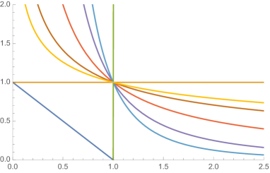
Figure 1: Left plot: Zeroes of the RHS in the $x,\,y$ plane compared with the zero of the LHS (the diagonal of the square). Right plot: The error of the 3-d order approximation vs $x,\,y$. The unit is $\frac{1}{\kappa}$.

3 The loop formula for QCD with Wilson fermions in $d=2,\,4$.

For definitness we give here the Wilson fermion matrix in $d=2,\,4$ for one flavour:

$$W = \hbox{1}-\kappa Q$$

$$= \hbox{1}-\kappa\sum_{i=1}^{d-1}\left(\Gamma_{+i}\,U_{i}\,T_{i}+\Gamma_{-i}\,T^{-1}_{i}\,U^{-1}_{i}\right)-\kappa\left(\rm e\,^{\mu}\,\Gamma_{+d}\,U_{d}\,T_{d}+\rm e\,^{-\mu}\,\Gamma_{-d}\,T^{-1}_{d}\,U^{-1}_{d}\right)\,$$

$$\Gamma_{\pm\nu} = 1\pm\gamma_{\nu},\,\gamma_{\nu}=\gamma_{\nu}^{*},\,\gamma_{\nu}^{2}=1,\,\hbox{tr}\Gamma_{\pm\nu}=d,$$ (6)

($T$: lattice translations, $\kappa$: hopping parameter, $\mu$ chemical potential). For latter generalisation we take the links $U_{\nu}\in SL(3,C)\supset SU(3)$.

The loop expansion and the loop formula for $\hbox{Det}\,W$ are

$$\hbox{Det}\,W = \hbox{Det}(\hbox{1}-\kappa Q)=\rm e\,^{\hbox{Tr}\,\ln(\hbox{1}-\kappa Q)}$$ (7)

$$= {\rm exp}\left[-\sum_{l=1}^{\infty}\sum_{\left\{{\cal C}_{l}\right\}}\sum_{s=1}^{\infty}~{}{{{g_{{\cal C}_{l}}}^{s}}\over s}\,\hbox{tr}_{\rm D,C}\left[{\cal L}_{{\cal C}_{l}}^{s}\right]\right]$$ (8)

$$= \prod_{l=1}^{\infty}~{}\prod_{\left\{{\cal C}_{l}\right\}}\det_{\rm D,C}\left(\hbox{1}~{}-~{}g_{{\cal C}_{l}}{\cal L}_{{\cal C}_{l}}\right)\,\,,$$ (9)

$$g_{{\cal C}_{l}} = \kappa^{l}\,\left(\epsilon\,\rm e\,^{N_{d}\mu}\right)^{r},\ {\cal L}_{{\cal C}_{l}}=\prod_{\lambda\in{\cal C}_{l}}\Gamma_{\lambda}U_{\lambda}.$$ (10)

Here ${\cal C}_{l}$ are distinguishable, non-exactly-self-repeating lattice closed paths of length $l$ (called primary paths in the follwing). $r$ is the net winding number of the path in the time direction ($d$), with p.b.c. or a.p.b.c. and $\epsilon=+1(-1)$ correspondingly ( p.b.c. in the ‘spatial’ directions). $\hbox{Det},\,\hbox{Tr}$ imply Lattice, Dirac, and colour d.o.f., ${\cal L}_{{\cal C}_{l}}^{s}\equiv\left({\cal L}_{{\cal C}_{l}}\right)^{s}$ is the chain of links and $\Gamma$ factors along a primary path (a primary loop), closing under the trace after $s$ repeted coverings of the path ${\cal C}_{l}$. From Eq. (8) to (9) we used “s-resummation”.

Derivation:
$Q$ implies unit steps on the lattice and $Q^{n}$ generates a (closed) path of length $n$, with the weight $\frac{1}{n}$. This can be the $s$ repetion of a closed path of length $l$ - a primary path. The primary path can start cyclically at each of its points, has therefore multiplicity $l$, its repetitions do not bring new paths. (NB: Pauli’s principle was used obtaining the determinant, after that it’s matrix algebra.)

The colour and Dirac traces close over the whole chain of length $ls$, the $s$ power of the primary loop ${\cal L}_{{\cal C}_{l}}$ Eq. (10) and do not depend on the starting point of the latter. Their contribution comes therefore with the weight $\frac{l}{ls}=\frac{1}{s}$ and the factor $g_{{\cal C}_{l}}$ coming from the links - see Eq. (8). We recognize here the logarithm series, and partial summations over $s$ and exponentiation lead to Eq. (9).

The loops in Eq. (10) can be rewritten as

$${\cal L}_{{\cal C}_{l}} = \Gamma_{{\cal C}_{l}}U_{{\cal C}_{l}},\ \Gamma_{{\cal C}_{l}}=\prod_{\lambda\in{\cal C}_{l}}\Gamma_{\lambda},\ U_{{\cal C}_{l}}=\prod_{\lambda\in{\cal C}_{l}}U_{\lambda}\$$

$$\hbox{tr}_{D,C}{\cal L}_{{\cal C}_{l}}^{s}=\hbox{tr}_{D}\Gamma_{{\cal C}_{l}}^{s}\,\hbox{tr}_{C}U_{{\cal C}_{l}}^{s}\equiv\hbox{tr}\left(\Gamma_{{\cal C}_{l}}\right)^{s}\,\hbox{tr}\left(U_{{\cal C}_{l}}\right)^{s}$$

since the Dirac and colour traces factorise. The Dirac factors $\hbox{tr}\Gamma_{{\cal C}_{l}}^{s}\equiv\hbox{tr}_{D}\Gamma_{{\cal C}_{l}}^{s}$ can be calculated for each ${\cal C}_{l}$ geometrically [7] or numerically.

For loops exploring up to three dimensions we have moreover [7]

$$\frac{2}{d}\,\hbox{tr}\left[\Gamma_{{\cal C}_{l}}\right]^{s}=\left[\frac{2}{d}\,\hbox{tr}\Gamma_{{\cal C}_{l}}\right]^{s}=h_{{\cal C}_{l}}^{s}$$ (12)

which simplifies the contributions of these loops to

$$\det_{C}(1-g_{{\cal C}_{l}}h_{{\cal C}_{l}}U_{{\cal C}_{l}})=(1+C_{{\cal C}_{l}}^{3})(1+a\,\hbox{tr}U_{{\cal C}_{l}}+b\,\hbox{tr}U_{{\cal C}_{l}}^{-1}),$$ (13)

$$C_{{\cal C}_{l}}=g_{{\cal C}_{l}}h_{{\cal C}_{l}},\ a=\frac{C_{{\cal C}_{l}}}{(1+C_{{\cal C}_{l}}^{3})},\ b=a\,C_{{\cal C}_{l}}$$ (14)

4 Applications

4.1 HD-QCD

For QCD at chemical potential $\mu>0$ the coefficients of primary loops of length $l$ with positive net winding number $r>0$ in the time direction are

$$g_{{\cal C}_{l}}=\kappa^{l_{\sigma}}\epsilon^{r}\zeta^{rN_{\tau}},\,\ l_{\sigma}=l-r\,N_{\tau}\geq 0,\,\ \zeta=\frac{d}{2}\kappa\rm e\,^{\mu}$$ (15)

Here $d=2,4$, $\epsilon=\mp 1$ for (a.)p.b.c.. Since $\zeta$ and $\kappa$ play different roles we order the contributions according to $l_{\sigma}$.

HD-QCD in leading order (LO, $l_{\sigma}=0$) ensues in the limit [9]

$$\kappa\rightarrow 0,\,\ \mu\rightarrow\infty,\,\ \zeta:fixed$$ (16)

It describes gluon dynamics with static quarks. Only the straight Polyakov loops $P$ in Eq. (9) survive. With $l_{\sigma}=2$ we retrieve Polyakov loops with one decoration, $\tilde{P}$, and the quarks have some mobility - [8]. The corresponding contributions are of the form Eq. (14), with

$$C_{P}\equiv C=\epsilon(\frac{d}{2}\zeta)^{N_{\tau}},\ \ C_{\tilde{P}}\equiv C_{r}=\kappa^{2}C^{r},$$ (17)

respectively. The decoration can be inserted anywhere along the Polyakov loop and have any length. There are therefore $2(d-1)N_{\tau}(N_{\tau}-1)$ primary decorated loops of length $l=N_{\tau}+2$. From each of them we can form, however, further primary loops of order $\kappa^{2}$ by attaching or inserting any number $r>1$ of straight Polyakov loops to obtain .

We obtain to this order (up to a constant factor)

$$\det W^{[2]}=\prod_{\vec{x}}(1+a\,\hbox{tr}P_{\vec{x}}+b\,\hbox{tr}P_{\vec{x}}^{-1})\ \,\prod_{q}\prod_{r\geq 1}(1+a_{r}\,\hbox{tr}{\tilde{P}}_{q,r,\vec{x}}+b_{r}\,\hbox{tr}{\tilde{P}}_{q,r,\vec{x}}^{-1}),$$ (18)

$$a=C(1+C^{3})^{-1},\ b=a\,C,\ \ a_{r}=C_{r}(1+C_{r}^{3})^{-1},\ b_{r}=a_{r}\,C_{r}$$ (19)

Here $q$ identifies the $2(d-1)N_{\tau}(N_{\tau}-1)$ shortest decorated Polyakov loops. The second factor in Eq. (18), however, is an infinite product. For $\kappa$ small enough to ensure convergence we can cut the product, e.g. at $r=1$, this was done in [8] for a reweighting simulation to produce the phase diagram of QCD with 3 flavours of heavy quarks.

4.2 Complex Langevin Simulation

The CL process associated to a partition function $Z$ with complex measure proceeds in the manifold of a complex variable $z$ and involves a drift force $K$ as the logarithmic derivative of the measure

$$Z=\int dz\,\rho(z),\ \ \delta z(t)=K(z)\delta t+\omega(z,t),\ \ K(z)=\frac{\rho^{\prime}(z)}{\rho(z)},$$ (20)

with $\omega$ an appropriately normalized random noise.

A CL process to simulate QCD at nonzero $\mu$ takes place in the complexified space of the link variables $U\in SL(3,C)$ [11], [12]. The drift incorporates the logarithmic derivative of the determinant and needs the evaluation of the inverse of $W$, Eq. (3) which is a large matrix of rang $N_{\sigma}^{d-1}N_{\tau}N_{c}d$.

Using the loop formula Eq. (9) we have

$$K(U_{\lambda})=\sum_{\left\{{\cal C}_{\lambda}\right\}}\frac{\partial_{U_{\lambda}}\det_{\rm D,C}\left(\hbox{1}~{}-~{}g_{{\cal C}_{\lambda}}{\cal L}_{{\cal C}_{\lambda}}\right)}{\det_{\rm D,C}\left(\hbox{1}~{}-~{}g_{{\cal C}_{\lambda}}{\cal L}_{{\cal C}_{\lambda}}\right)}$$ (21)

where the sum involves all loops ${\cal L}_{\lambda}$ which contain the link $U_{\lambda}$ and the terms are easily calculable. There are of course infinitely many such loops and they may also contain powers of $U_{\lambda}$, a simulation on these lines can only be achieved if we can meaningfully limit the number of terms in Eq. (21).

5 Two more simple examples

For illustration we present here 2 simple examples: a 1-d a.p.b.c. chain and a $2\times 2$ lattice with free b.c.in one direction and (a.)p.b.c. (for $\epsilon=\mp 1$, respectively) in the other direction - see Fig. 2.

Figure 2: Chain (left plot) and $2\times 2$ lattice without gauge fixing (middle) and in maximal gauge (right plot).

The chain has only one primary loop $P=U_{1}\,U_{2}$ and the loop formula reproduces the exact $\det W$

$$\det W=1+4\zeta^{2}P+4\kappa^{4}\zeta^{-2}P^{-1}+16\kappa^{4}$$ (22)

A similar result holds also for Polyakov loops of any length with a correspondig power of $\zeta^{2}$.

In the $2\times 2$ lattice example there are 12 primary loops of length $l\leq 6$, listed here with their weights

$$L_{1,2}: U_{1}U_{2},\ V_{1}V_{2}, (4\epsilon\zeta^{2}),$$ (23)

$$L_{3,4}: S_{1}V_{1}S_{2}^{-1}U_{1}^{-1},\ S_{2}V_{2}S_{1}^{-1}U_{2}^{-1},\, (-4\kappa^{4}),$$ (24)

$$L_{5,6}: S_{1}V_{1}S_{2}^{-1}U_{2},\ S_{2}V_{2}S_{1}^{-1}U_{1},\, (4\epsilon\zeta^{2}\kappa^{2}),$$ (25)

$$L_{7-9}: S_{1}V_{1}V_{2}V_{1}S_{2}^{-1}U_{2},\ S_{2}V_{2}S_{1}^{-1}U_{1}U_{2}U_{1},\ S_{1}V_{1}V_{2}V_{1}S_{2}^{-1}U_{2},\ (-16\zeta^{4}\kappa^{2}),$$ (26)

$$L_{10-12}: S_{2}V_{2}V_{1}V_{2}S_{1}^{-1}U_{1},\ S_{1}V_{1}V_{2}S_{1}^{-1}U_{1}U_{2},\ S_{2}V_{2}V_{1}S_{2}^{-1}U_{2}U_{1},\ (-16\zeta^{4}\kappa^{2})$$ (27)

The loop formula keeping only the loops of length up to 6 gives to 2-nd order in $\kappa$ (in maximal gauge)

$$D^{[0]}(1,2)=1-4\epsilon\zeta^{2}(U+V)+16\zeta^{4}U\,VD^{[2]}(3-6)=-4\epsilon\kappa^{2}\zeta^{2}(V\,X+U\,X^{-1})$$ (28)

$$D^{[2]}(7-12)=1-16\kappa^{2}\zeta^{4}(2\,U\,V+X\,V\,U+X^{-1}U\,V+X^{-1}U^{2}+X\,V^{2}))$$ (29)

and we obtain the determinant to order $\kappa^{2}$ including all loops up to length 6, in complete agreement with the exact determinant to this order

$$\det W^{[2,6]}=1-4\epsilon\zeta^{2}(U+V)+16\zeta^{4}U\,V-4\epsilon\zeta^{2}\kappa^{2}(V\,X+U\,X^{-1})-32\zeta^{4}\kappa^{2}U\,V$$ (30)

6 Discussion

As appealing as the loop formula appears its use is involved. The formula does not allow an interpretation as “linear factors” decomposition, but provides a systematic approximation in $\kappa$ approaching the true determinant in the convergence domain. As we have seen in sect. 1, leaving the latter will provide a rather poor approximation.

On the other hand we can see the various orders in the loop expansion as models by themselves and may analyse their properties. In that case we have however to introduce some way of limiting the number of loops at any given length, e.g. in a random walk generation of such loops.

The usefulness of the loop formula relies therefore on its correct interpretation and adequate use.

Acknowledgment: Support from the Deutsche Forschungsgemeinschaft in the frame of the project STA 283/16-2 is thankfully acknowledged.

References

• [1] W. Heisenberg and H. Euler, Z. Phys.  98 (1936) 714 [physics/0605038].
• [2] J. S. Schwinger, Phys. Rev.  82 (1951) 664.
• [3] E. Seiler, in: Proceedings of the International Summer School of Theoretical Physics, Poiana Brasov, Romania, 1981, edited by P. Dita, V. Georgescu, and R. Purice, Progress in Physics (Birkhäuser, Boston, 1982), Vol. 5, p. 263-310.
• [4] M. P. Fry, Phys. Rev. D 91 (2015) 085026 [arXiv:1504.03117 [hep-th]].
• [5] K. Langfeld, L. Moyaerts and H. Gies, Nucl. Phys. B 646 (2002) 158 [hep-th/0205304].
• [6] M. G. Schmidt and I. Stamatescu, Mod. Phys. Lett. A 18 (2003) 1499.
• [7] I.-O. Stamatescu, Phys. Rev. D 25 (1982) 1130.
• [8] R. De Pietri, A. Feo, E. Seiler, I.-O. Stamatescu, Phys. Rev. D 76 (2007) 114501
• [9] I. Bender, T. Hashimoto, F. Karsch, V. Linke, A. Nakamura, M. Plewnia, I.-O. Stamatescu and W. Wetzel, N.Ph.  Proc.S.  26 (1992) 323.
• [10] E. Seiler and I.-O. Stamatescu, J. Phys. A  Math. and General 2016 on-line, [arXiv:1512.07480v3]
• [11] G. Aarts, L. Bongiovanni, E. Seiler, D. Sexty, I.-O. Stamatescu, Eur. Phys. J. A 49 (2013) 89
• [12] G. Aarts, E. Seiler, D. Sexty and I.-O. Stamatescu, Phys. Rev. D 90 (2014) no.11, 114505