Modal analysis of masonry structures

Abstract

This paper presents a new numerical tool for evaluating the vibration frequencies and mode shapes of masonry buildings in the presence of cracks. The algorithm has been implemented within the NOSA-ITACA code, which models masonry as a nonlinear elastic material with zero tensile strength. Some case studies are reported, and the differences between linear and nonlinear behaviour highlighted.

1 Introduction

The worldwide architectural heritage is in pressing need of maintenance and restoration. Old structures are, in fact, threatened by numerous environmental and anthropogenic actions. In Italy, where seismic actions affect most of the territory, safeguarding ancient masonry buildings and monuments is a crucial issue for institutions and individuals alike. In this context, the use of non–destructive techniques able to evaluate the structural health of old buildings has a vital role to play.

Traditional building monitoring protocols generally involve visual inspections and the measurement of some quantities (displacements, local stresses and crack width, etc.) and their variation in time, while the mechanical properties of the constituent materials are generally assessed locally through destructive or non–destructive tests. More recently ambient vibration tests, first adopted in civil engineering to assess the structural health of bridges and tall buildings, have assumed an increasingly important place in the fields of conservation and restoration. This is for the most part due to the availability of very sensitive measurement devices and ever more powerful techniques for numerical simulation. These tests allow measuring structures’ dynamic properties, such as natural frequencies, mode shapes and damping ratios and, if coupled with a finite–element model, can provide important information on the mechanical properties of a building’s constituent materials and boundary conditions. Moreover, long–term monitoring protocols allow measuring any variation in the dynamic behaviour of the monitored structures: once the influence of environmental factors such as temperature and humidity has been accounted for, this variation can reveal the presence of any structural damage. Particular attention must be devoted in the monitoring of old masonry buildings, since their make–up and behaviour are profoundly different from modern structures. In fact, masonry is unable to withstand tensile stresses or large compressive stresses. For this reason, old buildings generally present damage scenarios, with cracking induced by the permanent loads or caused by some accidental events occurred during their long history. The dynamic behaviour of these structures should be analyzed taking into account the existing damage.

Numerous examples can be found in the literature of methods for detecting the effects of damage on the dynamic properties of structures. A number of analytical models have been formulated for predicting the effects of cracks on the vibration frequencies of beams and rotors [1]. A review of methods for detecting structural damage by measuring the changes over time of the natural frequencies is presented in [2]. Changes in mode shapes are effective damage indicators [3], [4] and allow better localization of the damage location within the structure. In particular, modal curvatures seem to be very sensitive to local damage [5], though their measurement requires the use of a large number of sensors. Wide variations in modal parameters can be observed when damage occurs in zones with high modal curvatures. With regard to the monitoring of old masonry structures, a number of papers have recently been devoted to the analysis of data from long–term monitoring protocols; these have highlighted changes in the modal characteristics due to environmental factors [6], [7], [8], or, in some cases, structural damage [9], [10], [11], [12].

Much effort has also been devoted to numerically simulating the effects of damage on the vibrations of the structures. In [13] and [14] a damage identification procedure is presented to detect and localize damage in beam structures. A beam is discretized into finite–elements and the damage to it simulated by reducing the stiffness matrix of some selected elements via a damage index. The equations obtained enable obtaining the beam’s frequencies and mode shapes when the damage indices are fixed or, viceversa, calculating the damage indices when frequencies and mode shapes are measured on real beams. Model updating procedures are employed in [15] in order to fit experimental data with finite–element models; the parameters to be updated are the Young’s moduli of the constituent materials. With regard to masonry buildings, a common approach consists of simulating the existing damage actually observed on the structure, by reducing the stiffness of those elements of the finite element model belonging to the cracked or damaged parts [16], [10]. In [17] and [18] the dynamic properties of some masonry structures at different damage levels are investigated via the discrete element method.

The work presented in [19] formulates an explicit expression linking the fundamental frequency of a masonry–like beam to its maximum transverse displacement. The masonry–like constitutive equation models masonry as a non–linear elastic material with different strengths under tension and compression [20], [21]. This constitutive equation has been implemented in the finite–element code NOSA for the static analysis of masonry bodies [22]. The NOSA code and its updated version NOSA–ITACA 1.0 [23], have been applied to the static and dynamic analysis of many important monuments in Italy. NOSA–ITACA 1.0 is freely downloadable at [24]. The non–linear equilibrium equations of masonry–like bodies are solved via the Newton–Raphson method, by taking into account an explicit expression of the derivative of the stress with respect to the strain [22], which allows calculation of the system’s tangent stiffness matrix.

This paper presents a numerical procedure, implemented in a newly updated version 1.2 of the NOSA–ITACA code, which can evaluate the natural frequencies and mode shapes of masonry buildings in the presence of cracks. Once the initial loads and boundary conditions have been applied to the finite–element model, the resulting non–linear equilibrium problem is solved through an iterative scheme. Then, a modal analysis is performed, by using the tangent stiffness matrix calculated by the code in the last iteration before convergence is reached. The incremental approach used by NOSA–ITACA 1.2 allows the user to perform the modal analysis at the initial step, before application of any load to the structure, and then for different loading steps. Following the prestressed modal analysis applied to problems with geometric nonlinearity [25] and [26], the proposed procedure allows the user to automatically take into account the stress distribution on the system’s stiffness matrix, thereby evaluating the effects of the presence of cracked and crushed material on the structure’s dynamic properties.

Section 2 briefly recalls the constitutive equation of masonry–like materials. The explicit expressions for the stress function and its derivative, obtained in [22], are summarized, and the numerical procedure for solving static and dynamic problems of masonry structures, implemented in the NOSA–ITACA 1.0 code, are sketched out. Finally, the modal analysis of linear elastic structures is addressed and the procedures implemented in the NOSA–ITACA 1.0 code to solve the constrained generalized eigenvalue problem resulting from application of the finite-element method is outlined [27]. Section 3 presents the new procedure implemented in the NOSA–ITACA 1.2 code. The code allows for calculating the natural frequencies and mode shapes of a masonry body subjected to prescribed boundary conditions and loads. The new procedure takes into account the non–linearity of the constitutive equation of masonry–like materials as well as the presence of cracks due to the applied loads. In general, the results of the modal analysis conducted after application of the assigned loads differ from those obtained via the standard modal analysis and can be used to assess the presence of damaged zones in the structure. Section 4 presents some applications of the method. The first two cases deal with a masonry beam and an arch on piers. Both structures are subjected to incremental loads and analyzed with the NOSA–ITACA code. The aim is to compare the natural frequencies and mode shapes in the linear elastic case with those calculated in the presence of the crack distribution induced by the increasing loads. The third case deals with an actual structure, the bell tower of San Frediano in Lucca. The tower has been instrumented with four high–sensitivity triaxial seismometric stations [28], and its first five natural frequencies have been determined via OMA techniques [29]. Then the NOSA–ITACA code, together with model updating techniques, has been employed in order to fit the experimental results. The model updating in the linear elastic case is compared to the model updating applied to the tower subjected to its own weight by taking into account the crack distribution induced by the loads.

2 The masonry–like constitutive equation and the NOSA-ITACA 1.0 code

Let $Lin$ be the set of all second-order tensors with the scalar product $\mathbf{A}\cdot\mathbf{B}=tr(\mathbf{A}^{T}\mathbf{B})$ for any $\mathbf{A},\mathbf{B}\in$ $Lin$, with $\mathbf{A}^{T}$ the transpose of $\mathbf{A}$. For $Sym$ the subspace of symmetric tensors, $Sym^{-}$ and $Sym^{+}$ are the sets of all negative-semidefinite and positive-semidefinite elements of $Sym$. Given the symmetric tensors $\mathbf{A}$ and $\mathbf{B}$, we denote by $\mathbf{A}\otimes\mathbf{B}$ the fourth-order tensor defined by $\mathbf{A}\otimes\mathbf{B}[\mathbf{H}]=(\mathbf{B}\cdot\mathbf{H})\mathbf{A}$ for $\mathbf{H}\in Lin$ and by $\mathbb{I}_{Sym}$ the fourth-order identity tensor on $Sym$. For $\mathbf{a}$ and $\mathbf{b}$ vectors, the dyad $\mathbf{a}\otimes\mathbf{b}$ is defined by $\mathbf{a}\otimes\mathbf{bh}=(\mathbf{b}\cdot\mathbf{h})\mathbf{a},$ for any vector $\mathbf{h}$, with $\cdot$ the scalar product in the space of vectors.

Let $\mathbb{C}$ be the isotropic fourth-order tensor of elastic constants

$$\mathbb{C}=2\mu\mathbb{I}_{Sym}+\lambda\mathbf{I}\otimes\mathbf{I},$$ (1)

where $\mathbf{I}\in Sym$ is the identity tensor and $\mu$ and $\lambda$ are the Lamé moduli of the material satisfying the conditions

$$\mu>0,\textup{ \ \ }\lambda\geq 0.$$ (2)

$\mathbb{C}$ is symmetric,

$$\mathbf{A}\cdot\mathbb{C}[\mathbf{B}]=\mathbf{B}\cdot\mathbb{C}[\mathbf{A}],\,\,\,\,\textup{for all}\,\,\,\,\mathbf{A},\mathbf{B}\in Sym,$$ (3)

and in view of (2) is positive-definite on $Sym$,

$$\mathbf{A}\cdot\mathbb{C}[\mathbf{A}]>0\,\,\,\,\textup{for all}\,\,\,\,\mathbf{A}\in Sym,\,\,\,\,\mathbf{A}\neq 0.$$ (4)

A masonry-like material is a nonlinear elastic material [22] characterized by the fact that, for $\mathbf{E}\in Sym$, there exists a unique triplet $(\mathbf{T},\mathbf{E}^{e},\mathbf{E}^{f})$ of elements of $Sym$ such that

$$\mathbf{E}=\mathbf{E}^{e}+\mathbf{E}^{f},$$ (5)

$$\mathbf{T}=\mathbb{C}[\mathbf{E}^{e}],$$ (6)

$$\mathbf{T}\in Sym^{-},\textup{ \ \ }\mathbf{E}^{f}\in Sym^{+},$$ (7)

$$\mathbf{T}\cdot\mathbf{E}^{f}=0.$$ (8)

$\mathbf{T}$ is the Cauchy stress corresponding to strain $\mathbf{E}$. Tensors $\mathbf{E}^{e}$ and $\mathbf{E}^{f}$ are respectively the elastic and inelastic part of $\mathbf{E}$; $\mathbf{E}^{f}$ is also called the fracture strain. The stress function $\mathbb{T}:Sym\rightarrow Sym$ is given by

$$\mathbb{T}(\mathbf{E})=\mathbf{T},\,\,\,\,\textup{for any \ \ }\mathbf{E}\in Sym,$$ (9)

with $\mathbf{T}$ satisfying (5)–(8). The explicit expression for the stress function $\mathbb{T}$, calculated in [22], is recalled in the following.

For $\mathbf{E}\in Sym,$ let $e_{1}\leq e_{2}\leq e_{3}$ be its ordered eigenvalues and $\mathbf{q}_{1},$ $\mathbf{q}_{2},\mathbf{q}_{3}$ the corresponding eigenvectors. We introduce the orthonormal basis of $Sym$ (with respect to the scalar product $\cdot$)

$$\mathbf{O}_{11}=\mathbf{q}_{1}\otimes\mathbf{q}_{1},\textup{ }\mathbf{O}_{22}=\mathbf{q}_{2}\otimes\mathbf{q}_{2},\textup{ }\mathbf{O}_{33}=\mathbf{q}_{3}\otimes\mathbf{q}_{3},\textup{ }$$

$$\mathbf{O}_{12}=\frac{1}{\sqrt{2}}(\mathbf{q}_{1}\otimes\mathbf{q}_{2}+\mathbf{q}_{2}\otimes\mathbf{q}_{1}),\textup{ }\mathbf{O}_{13}=\frac{1}{\sqrt{2}}(\mathbf{q}_{1}\otimes\mathbf{q}_{3}+\mathbf{q}_{3}\otimes\mathbf{q}_{1}),$$ (10)

$$\mathbf{O}_{23}=\frac{1}{\sqrt{2}}(\mathbf{q}_{2}\otimes\mathbf{q}_{3}+\mathbf{q}_{3}\otimes\mathbf{q}_{2}).$$

Given $\mathbf{E}$, the corresponding stress $\mathbf{T}$ satisfying the constitutive equation of masonry-like materials (5)–(8) is given by

$$\textup{if }\mathbf{E}\in V_{0}\textup{ then }\mathbf{T}=\mathbf{0},$$ (11)

$$\textup{if }\mathbf{E}\in V_{1}\textup{ then }\mathbf{T}=Ee_{1}\mathbf{O}_{11},$$ (12)

$$\textup{if }\mathbf{E}\in V_{2}\textup{ then }\mathbf{T}=\frac{2\mu}{2+\alpha}\left\{[2(1+\alpha)e_{1}+\alpha e_{2}]\mathbf{O}_{11}\right.$$

$$\left.+[\alpha e_{1}+2(1+\alpha)e_{2}]\mathbf{O}_{22}\right\},$$ (13)

$$\textup{if }\mathbf{E}\in V_{3}\textup{ then }\mathbf{T}=\mathbb{C}[\mathbf{E}],$$ (14)

where the sets $V_{k}$ are

$$V_{0}=\left\{\mathbf{E}\in Sym\textup{ : }e_{1}\geq 0\right\},$$ (15)

$$V_{1}=\left\{\mathbf{E}\in Sym\textup{ : }e_{1}\leq 0,\textup{ }\alpha e_{1}+2(1+\alpha)e_{2}\geq 0\right\},$$ (16)

$$V_{2}=\left\{\mathbf{E}\in Sym\textup{ : }\alpha e_{1}+2(1+\alpha)e_{2}\leq 0,\textup{ }2e_{3}+\alpha tr\mathbf{E}\geq 0\right\},$$ (17)

$$V_{3}=\left\{\mathbf{E}\in Sym\textup{ : }2e_{3}+\alpha tr\mathbf{E}\leq 0\right\},$$ (18)

with $\alpha=\lambda/\mu$ and $E=\mu(2\mu+3\lambda)/(\mu+\lambda)$ the Young’s modulus.

As for the fracture strain,

$$\textup{if }\mathbf{E}\in V_{0}\textup{ then }\mathbf{E}^{f}=\mathbf{E},$$ (19)

$$\textup{if }\mathbf{E}\in V_{1}\textup{ then }\mathbf{E}^{f}=(e_{2}+\frac{\alpha}{2(1+\alpha)}e_{1})\mathbf{O}_{22}+(e_{3}+\frac{\alpha}{2(1+\alpha)}e_{1})\mathbf{O}_{33},$$ (20)

$$\textup{if }\mathbf{E}\in V_{2}\textup{ then }\mathbf{E}^{f}=[e_{3}+\frac{\alpha}{2+\alpha}(e_{1}+e_{2})]\mathbf{O}_{33},$$ (21)

$$\textup{if }\mathbf{E}\in V_{3}\textup{ then }\mathbf{E}^{f}=\mathbf{0}.$$ (22)

For $W_{k}$ the interior of $V_{k}$, function $\mathbb{T}$ turns out to be differentiable in $W=\bigcup\limits_{i=0}^{3}W_{i}$ [22],[30]. Thus, for $\mathbf{E}\in W$ denoting by $D_{E}\mathbb{T}(\mathbf{E})$ the derivative of $\mathbb{T}(\mathbf{E})$ with respect to $\mathbf{E}$, we have

$$\mathbb{T}(\mathbf{E}+\mathbf{H})=\mathbb{T}(\mathbf{E})+D_{E}\mathbb{T}(\mathbf{E})[\mathbf{H}]+o(\mathbf{H}),\text{ \ \ }\mathbf{H}\in Sym,\text{ \ \ }\mathbf{H}\rightarrow\mathbf{0}.$$ (23)

$D_{E}\mathbb{T}(\mathbf{E})$ is a symmetric fourth–order tensor from $Sym$ into itself and has the following expressions in the regions $W_{i}$ [22].

$$\textup{If }\mathbf{E}\in W_{0}\textup{ then }D_{E}\mathbb{T}(\mathbf{E})=\mathbb{O},$$ (24)

where $\mathbb{O}$ is the null fourth-order tensor,

$$\textup{if }\mathbf{E}\in W_{1}\textup{ then }D_{E}\mathbb{T}(\mathbf{E})=E\left(\mathbf{O}_{11}\otimes\mathbf{O}_{11}-\frac{e_{1}}{e_{2}-e_{1}}\mathbf{O}_{12}\otimes\mathbf{O}_{12}\right.$$

$$\left.-\frac{e_{1}}{e_{3}-e_{1}}\mathbf{O}_{13}\otimes\mathbf{O}_{13}\right),$$ (25)

$$\textup{if }\mathbf{E}\in W_{2}\textup{ then }D_{E}\mathbb{T}(\mathbf{E})=2\mu\mathbf{O}_{12}\otimes\mathbf{O}_{12}$$

$$-\frac{2\mu}{2+\alpha}\frac{2(1+\alpha)e_{1}+\alpha e_{2}}{e_{3}-e_{1}}\mathbf{O}_{13}\otimes\mathbf{O}_{13}$$

$$-\frac{2\mu}{2+\alpha}\frac{\alpha e_{1}+2(1+\alpha)e_{2}}{e_{3}-e_{2}}\mathbf{O}_{23}\otimes\mathbf{O}_{23}$$

$$+\frac{2\mu(2+3\alpha)}{2+\alpha}\frac{\mathbf{O}_{11}+\mathbf{O}_{22}}{\sqrt{2}}\otimes\frac{\mathbf{O}_{11}+\mathbf{O}_{22}}{\sqrt{2}}$$

$$+2\mu\frac{\mathbf{O}_{11}-\mathbf{O}_{22}}{\sqrt{2}}\otimes\frac{\mathbf{O}_{11}-\mathbf{O}_{22}}{\sqrt{2}},$$ (26)

$$\textup{if }\mathbf{E}\in W_{3}\textup{ then }D_{E}\mathbb{T}(\mathbf{E})=\mathbb{C}.$$ (27)

In order to study real problems, the equilibrium problem of masonry structures can be solved via the finite element method. To this end, suitable numerical techniques have been developed [22] based on the Newton-Raphson method for solving the nonlinear system obtained by discretising the structure into finite elements. Their application is based on the explicit expression for the derivative of the stress with respect to the strain, which is needed in order to calculate the tangent stiffness matrix. The numerical method studied and the constitutive equation of masonry-like materials described above have therefore been implemented into the finite element code NOSA [22].

As far as the numerical solution of dynamic problems is concerned, direct integration of the equations of motion is required [31]. In fact, due to the nonlinearity of the adopted constitutive equation, the mode-superposition method is meaningless. With the aim of solving such problems, we have instead implemented the Newmark method [32] within NOSA in order to perform the integration with respect to time of the system of ordinary differential equations obtained by discretising the structure into finite elements. Moreover, the Newton-Raphson scheme, needed to solve the nonlinear algebraic system obtained at each time step, has been adapted to the dynamic case. The NOSA code, devoted to static and dynamic analyses of ancient masonry constructions, enables determining the stress state and the presence of any cracking. Moreover, the effects of thermal variations and the effectiveness of various strengthening interventions, such as the application of tie rods and retaining structures, can be evaluated, and those with the least environmental and visual impact identified.

The code has been successfully applied to the analysis of arches and vaults [33], and in a number of studies of buildings of historical and architectural interest [22], [34].

Within the framework of the project ”Tools for modelling and assessing the structural behaviour of ancient constructions” [24] funded by the Region of Tuscany (2011-2013), the NOSA code has been integrated in the open source graphic platform SALOME [35], used both to define the geometry of the structure under examination and to visualise the results of the structural analysis. The result of this integration is the freeware code NOSA-ITACA 1.0 [23], [24]. NOSA-ITACA 1.0 has been applied to several studies commissioned by both private and public bodies of the static and dynamic behaviour of historical masonry buildings [36]. In many cases, such studies have also provided important information on the structure’s seismic vulnerability, which can be assessed with respect to current Italian and European regulations [37].

An efficient implementation of the numerical methods for constrained eigenvalue problems for modal analysis of linear elastic structures has been embedded in NOSA–ITACA 1.0 [27]. Such implementation takes into account both the sparsity of the matrices and the features of master-slave constraints (tying or multipoint constraints). It is based on the open-source packages SPARSKIT [38], for managing matrices in sparse format (storage, matrix-vector products), and ARPACK [39], which implements a method based on Lanczos factorization combined with spectral techniques that improve convergence. In particular in [27] the authors have implemented a procedure for solving the constrained generalized eigenvalue problem

$$K\,\phi=\omega^{2}\,M\,\phi,$$ (28)

$$T\phi=0,$$ (29)

with $T\in\mathbb{R}^{m\times n}$ and $m\ll n$. Equation (28) is derived from the equation

$$M\ddot{u}+Ku=0,$$ (30)

governing the free vibrations of a linear elastic structure discretized into finite elements. In equation (30) $u$ is the displacement vector, which belongs to $\mathbb{R}^{n}$ and depends on time $t$, $\ddot{u}$ is the second-derivative of $u$ with respect to $t$, and $K$ and $M\in\mathbb{R}^{n\times n}$ are the stiffness and mass matrices of the finite-element assemblage. $K$ is symmetric and positive-semidefinite, $M$ is symmetric and positive-definite, and both are banded with bandwidth depending on the numbering of the finite-element nodal points. Displacements $u_{i}$ are also called degrees of freedom; the integer $n$ is the total number of degrees of freedom of the system and is generally very large, since it depends on the level of discretization of the problem. By assuming that

$$u=\phi\sin(\omega t),$$ (31)

with $\phi$ a vector of $\mathbb{R}^{n}$ and $\omega$ a real scalar, and applying the modal superposition [32], equation (30) is transformed into the generalized eigenvalue problem (28). Condition (29) expresses the fixed constraints and the master-slave relations assigned to displacement $u$, written in terms of vector $\phi$. The restriction of the matrix $K$ to the null subspace of $\mathbb{R}^{n}$ defined by (29) is positive-definite.

Although the constitutive equation (5)–(8) adopted for masonry is nonlinear, the modal analysis, which is based on the assumption that the materials constituting the construction are linear elastic, is widely used in applications and furnishes important qualitative information on the dynamic behavior of masonry structures and thereby allows for assessing their seismic vulnerability in light of Italian and European regulations [37]. On the other hand, traditional modal analysis does not take into account the influence that both the nonlinear behaviour of the masonry material and the presence of cracked regions can have on the natural frequencies of masonry structures. The approach described in the next section and implemented in NOSA–ITACA 1.2 allows for calculating the natural frequencies and modal shapes of a masonry body subjected to given system of loads and exhibiting a crack distribution due to these loads.

3 A new procedure for the modal analysis of masonry–like structures

Let us consider a body $\mathcal{B}$ whose boundary $\partial\mathcal{B}$ is composed of two complementary and disjoined portions $\partial\mathcal{B}_{1}$ and $\partial\mathcal{B}_{2}$. $\mathcal{B}$ is made of a masonry-like material with constitutive equation (5)–(8) and mass density $\rho$. Given the loads ($\mathbf{b}$, $\mathbf{s_{0}}$), with the body force $\mathbf{b}$ defined over $\mathcal{B}$ and the surface force $\mathbf{s_{0}}$ defined over $\partial\mathcal{B}_{2}$, let ($\mathbf{\widetilde{u}}$, $\mathbf{\widetilde{E}}$, $\mathbf{\widetilde{T}}$) a triple consisting of one vector and two tensor fields defined over $\mathcal{B}$ satisfying the following equilibrium problem [22]

$$div\mathbf{\widetilde{T}}+\mathbf{b}=\mathbf{0}\,\,\,\,\,\,\text{on}\,\,\mathcal{B},$$ (32)

$$\mathbf{\widetilde{E}}=\frac{\nabla\mathbf{\widetilde{u}}+\nabla\mathbf{\widetilde{u}}^{T}}{2}\,\,\,\,\,\,\text{on}\,\,\mathcal{B},$$ (33)

$$\mathbf{\widetilde{T}}=\mathbb{T}(\mathbf{\widetilde{E}})\,\,\,\,\,\,\text{on}\,\,\mathcal{B},$$ (34)

$$\mathbf{\widetilde{u}}=\mathbf{0}\,\,\,\,\,\,\text{on}\,\,\partial\mathcal{B}_{1},$$ (35)

$$\mathbf{\widetilde{T}}\mathbf{n}=\mathbf{s_{0}}\,\,\,\,\,\,\text{on}\,\,\partial\mathcal{B}_{2}.$$ (36)

The equilibrium problem (32)-(36) is dealt with in [22], where the uniqueness of its solution in terms of stress is proved and the iterative procedure implemented in the NOSA code to calculate a numerical solution is described in detail.

Let $(0,t_{0})$ denote a fixed interval of time; a motion of $\mathcal{B}$ is a vector field $\mathbf{u}$ defined on $\mathcal{B}\times(0,t_{0})$. The vector $\mathbf{u}(\mathbf{x},t)$ is the displacement of $\mathbf{x}$ at time $t$ and $\frac{\partial^{2}\mathbf{u}}{\partial t^{2}}$ its acceleration. Let us consider small motions $\mathbf{u}$ such that their gradient $\nabla\mathbf{u}$ is small, and $\mathbf{u}=\mathbf{0}$ on $\partial\mathcal{B}_{1}$.

For the displacement field $\mathbf{\widetilde{u}}+\mathbf{u}$, the strain field $\mathbf{\widetilde{E}}+\mathbf{E}$, with $\mathbf{E}=({\nabla\mathbf{u}+\nabla\mathbf{u}^{T}})/2$ and the stress field $\mathbb{T}(\mathbf{\widetilde{E}}+\mathbf{E})$, the equation of motion reads

$$div{\large(}\mathbb{T}(\mathbf{\widetilde{E}}+\mathbf{E}){\large)}+\mathbf{b}=\rho\frac{\partial^{2}(\mathbf{\widetilde{u}}+\mathbf{u})}{\partial t^{2}}\,\,\,\,\,\,\text{on}\,\,\mathcal{B}.$$ (37)

From (37), in view of (23) and (34), bearing in mind the equilibrium equation (32) and neglecting terms of order $o(\nabla\mathbf{u})$, we get the linearized equation of motion

$$div{\large(}D_{E}\mathbb{T}(\mathbf{\widetilde{E}})[\frac{\nabla\mathbf{u+}\nabla\mathbf{u}^{T}}{2}]{\large)}=\rho\frac{\partial^{2}\mathbf{u}}{\partial t^{2}}\,\,\,\,\,\,\text{on}\,\,\mathcal{B},$$ (38)

where the fourth-order tensor $\large D_{E}\mathbb{T}(\mathbf{\widetilde{E}})$ depends on $\mathbf{x}\in\mathcal{B}$.

Equation (38), governing the undamped free vibrations of $\mathcal{B}$ about the equilibrium state ($\mathbf{\widetilde{u}}$, $\mathbf{\widetilde{E}}$, $\mathbf{\widetilde{T}}$), is linear and via the application of the finite element method can be transformed into the equation

$$M\ddot{u}+\widetilde{K}u=0,$$ (39)

which is analogous to (30), though here the elastic stiffness matrix $K$, calculated using the elastic tensor $\mathbb{C}$, has been replaced by the damaged stiffness matrix $\widetilde{K}$, calculated using $\large D_{E}\mathbb{T}(\mathbf{\widetilde{E}})$, which takes into account the presence of cracks in body $\mathcal{B}$.

Thus, a new numerical method for the modal analysis of masonry constructions has been implemented in an updated version 1.2 of the NOSA-ITACA code. Given the structure under examination, discretized into finite elements, and given the mechanical properties of the masonry-like material constituting the structure, together with the kinematic constraints and loads acting on it, the procedure consists of the following steps.

Step 1. A preliminary modal analysis is conducted by assuming the the structure’s constituent material to be linear elastic. The generalized eigenvalue problem (28)-(29) is then solved and the natural frequencies $\text{f}_{\text{i}}^{l}=\omega_{\text{i}}^{l}/2\pi$ and mode shapes $\phi_{\text{i}}^{l}$ calculated.

Step 2. The equilibrium problem (32)-(36) is solved and its solution, ($\mathbf{\widetilde{u}}$, $\mathbf{\widetilde{E}}$, $\mathbf{\widetilde{T}}$), calculated. The fourth-order tensor $\large D_{E}\mathbb{T}(\mathbf{\widetilde{E}})$ needed to calculate the damaged stiffness matrix $\widetilde{K}$ to be used in the next step is evaluated by using (24)–(27).

Step 3. The generalized eigenvalue problem (28)-(29), with matrix $\widetilde{K}$ in place of the elastic stiffness matrix $K$, is solved and the natural frequencies $\text{f}_{\text{i}}=\omega_{\text{i}}/2\pi$ and mode shapes $\phi_{\text{i}}$ of the damaged structure calculated.

4 Case studies

4.1 The masonry beam

Let us consider the rectilinear beam illustrated in Figure 1, with length $l=$6\text{\,}\mathrm{m}$$, rectangular cross section of $$0.4\text{\,}\mathrm{m}$\times$1\text{\,}\mathrm{m}$$, subjected to the concentrated vertical load $P=$10^{6}\text{\,}\mathrm{N}$$ and a uniform lateral load. The beam, simply supported at its ends and forced to move in the $y-z$ plane, is discretized with $60$ beam elements [23]. The goal of the finite–element analysis, conducted with the NOSA–ITACA 1.2 code is to compare the natural frequencies and mode shapes of the beam in the linear elastic case with those in the presence of the damage induced by the increasing lateral load. We conducted a preliminary modal analysis by assuming the beam to be made of a linear elastic material with Young’s modulus $E=$3\cdot 10^{9}\text{\,}\mathrm{Pa}$$, Poisson’s ratio $\nu=0.2$ and mass density $\rho=$1800\text{\,}\mathrm{k}\mathrm{g}\mathrm{/}\mathrm{m}^{3}$$, for which we calculated the corresponding natural frequencies $\text{f}_{\text{i}}^{l}$ and mode shapes $\phi_{\text{i}}^{l}$. Then, by following the procedure outlined in Section 3, we incremented the lateral load and, at each increment, calculated the frequencies $\text{f}_{\text{i}}$ and modes $\phi_{\text{i}}$. The value of the lateral load applied to the beam was increased through seven increments from $9\cdot 10^{3}\text{\,}\mathrm{N}$ (which was able to induce the first crack in the beam’s midsection) to $15.75\cdot 10^{3}\text{\,}\mathrm{N}$. Table 1 reports the value of the lateral load and the corresponding natural frequencies. The first row summarizes the results of the linear elastic modal analysis. As outlined in Table 1, as the lateral load increases, the beam’s fundamental frequency decreases from the linear elastic value of $6.47\text{\,}\mathrm{Hz}$ to $3.71\text{\,}\mathrm{Hz}$, about one half its initial value. The other frequencies fall by up to thirty per cent. The frequencies ratio $\text{f}_{\text{i}}/\text{f}_{\text{i}}^{l}$ is reported in Figure 2. The Figure clearly shows that when the lateral load is applied, the fundamental frequency value falls faster than the other frequency values. This is due to the chosen lateral load distribution, which induces a deformation in the beam similar to the first mode shape. Table 1 also reports the values of the effective modal masses [41] calculated for the first six mode shapes. The modes are also shown in Figure 1, where the black line stands for the modes $\phi_{\text{i}}^{l}$ calculated for the linear elastic case, while the cyan line represents the modes $\phi_{\text{i}}$ calculated at the last increment of the analysis. It is worth noting that the first, second, fifth and sixth modes substantially maintain their shape, while some changes occur between the third and fourth mode: their frequency values are very similar, but in the linear elastic analysis the third mode has an axial direction, while the fourth mode has transverse direction. The nonlinear case shows that the masses of the third mode pass from the axial to the transverse direction, while for the fourth mode diverts from transverse to axial [42]. A small part of the total mass in the axial direction migrates towards the higher modes and is not shown in the Table.

In order to compare the mode shapes $\phi_{\text{i}}^{l}$ and $\phi_{\text{j}}$, we introduce the quantity

$$\text{MAC--}M(\phi_{\text{i}}^{l},\phi_{\text{j}})=\frac{|\phi_{\text{i}}^{l}\cdot M\phi_{\text{j}}|}{\sqrt{\phi_{\text{i}}^{l}\cdot M\phi_{\text{i}}}\sqrt{\phi_{\text{j}}^{l}\cdot M\phi_{\text{j}}}},$$ (40)

which measures the correlation between the $\text{i}-\text{th}$ linear elastic mode shape and the $\text{j}-\text{th}$ mode shape of the damaged structure. More precisely, if the MAC–$M$ value is close to unity, then the vectors $\phi_{\text{i}}^{l}$ and $\phi_{\text{j}}$ are nearly parallel with to respect to the scalar product in $\mathbb{R}^{n}$ induced by matrix $M$. Table 2 reports the quantities MAC–$M(\phi_{\text{i}}^{l},\phi_{\text{j}})$ calculated for i, j = 1, 2, …, 6, with $\phi_{\text{j}}$ the damaged mode shape calculated at the last load increment, corresponding to the lateral load $15.75\cdot 10^{3}\text{\,}\mathrm{N}$. As the lateral load increases, the quantities MAC–$M(\phi_{\text{3}}^{l},\phi_{\text{3}})$ and MAC–$M(\phi_{\text{3}}^{l},\phi_{\text{4}})$ drawn in Figure 3 in blue and green lines, respectively, pass from $1$ to $0.4$ and from $0$ to $0.88$ (see Table 2), thus showing that mode shape $\phi_{\text{3}}$, initially coincident with $\phi_{\text{3}}^{l}$, tends to become $M$-orthogonal to it and $\phi_{\text{4}}$ initially $M$-orthogonal to $\phi_{\text{3}}^{l}$ tends to become $M$-parallel to it. Finally, Figure 4 shows the distributions of the fractured areas in the beam at the last load increment, together with the ratio between the cracked area $\text{A}_{\text{f}}$ and total area A calculated in every section of the beam.

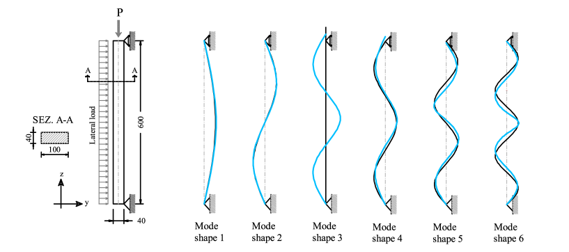
Figure 1: The geometry of the beam (left) and its first six mode shapes (right): linear elastic (black) and masonry–like (cyan) case (lengths in cm). The masonry–like case is shown for the last load increment.

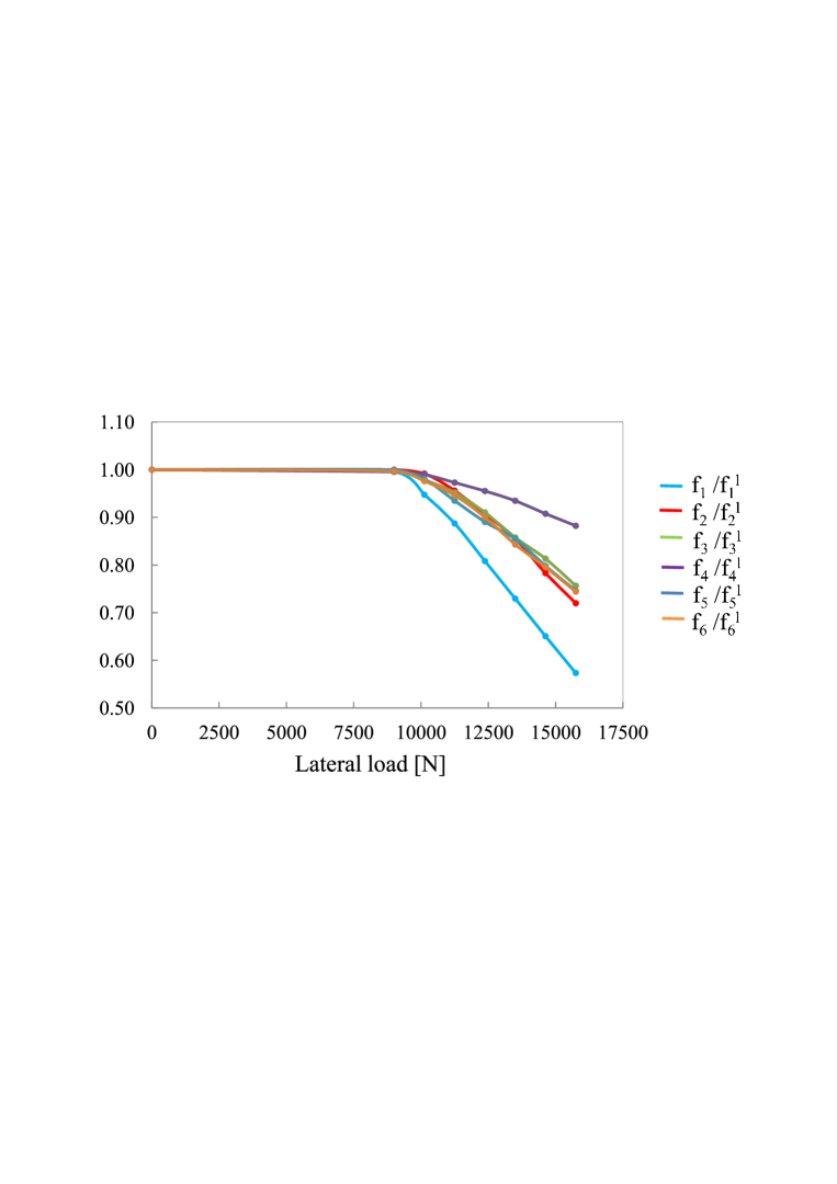
Figure 2: The ratio $\text{f}_{\text{i}}/{\text{f}_{\text{i}}}^{l}$ for the first six natural frequencies of the beam vs. the lateral load.

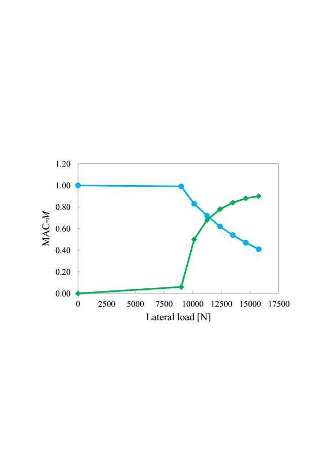
Figure 3: The quantities MAC–$M(\phi_{3}^{l},\phi_{3})$ (blue line) and MAC–$M(\phi_{3}^{l},\phi_{4})$ (green line) vs. the lateral load.

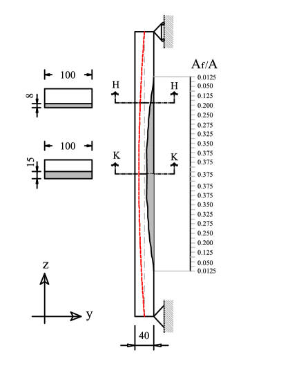
Figure 4: The ratio between the cracked area $\text{A}_{\text{f}}$ and total area A along the beam at the last load increment. (lengths in cm).

4.2 The masonry arch on piers

Let us consider the masonry arch on piers shown in Figure 5. The arch span is $6\text{\,}\mathrm{m}$ and its cross section measures $$0.25\text{\,}\mathrm{m}$\times$1\text{\,}\mathrm{m}$$. The arch has a circular shape, with a mean radius of $3.75\text{\,}\mathrm{m}$, and rests on two lateral piers with rectangular cross section of $$0.8\text{\,}\mathrm{m}$\times$1\text{\,}\mathrm{m}$$ and height $4\text{\,}\mathrm{m}$. The structure is reinforced by means of two steel tie rods, with rectangular cross sections of $$0.03\text{\,}\mathrm{m}$\times$0.03\text{\,}\mathrm{m}$$, fixed at the pier–arch nodes. An offset of $0.24\text{\,}\mathrm{m}$ has been considered between the axis of the arch and those of the piers. The structure, modelled by means of $1500$ thick shell elements, [23], [36], is clamped at the piers’ base and forced to move in the $x-z$ plane. Figure 5 also shows the elements’ local axes in red. Beam elements [23] have been used to model the tie rods.

Just as for the beam described in the previous subsection, we conducted a preliminary modal analysis by assuming the masonry structure to be made of a linear elastic material with Young’s modulus $E=$3\cdot 10^{9}\text{\,}\mathrm{Pa}$$, Poisson’s ratio $\nu=0.2$ and mass density $\rho=$1800\text{\,}\mathrm{k}\mathrm{g}\mathrm{/}\mathrm{m}^{3}$$, while for the tie rods we have assumed $E=$2.1\cdot 10^{11}\text{\,}\mathrm{Pa}$$, Poisson’s ratio $\nu=0.3$ and mass density $\rho=$7850\text{\,}\mathrm{k}\mathrm{g}\mathrm{/}\mathrm{m}^{3}$$. The modal analysis allowed us to calculate the structure’s natural frequencies $\text{f}_{\text{i}}^{l}$ and mode shapes $\phi_{\text{i}}^{l}$. The loads have been applied incrementally, first the self–weight of the structure alone, and then a concentrated vertical load P, whose value was increased through four increments from $150.61\cdot 10^{3}\text{\,}\mathrm{N}$ to $154.61\cdot 10^{3}\text{\,}\mathrm{N}$. Seven analyses were performed, each time moving the load P to different positions along the arch span (see Figure 5). The natural frequencies $\text{f}_{\text{i}}$ and mode shapes $\phi_{\text{i}}$ of the damaged structure have thus been calculated for each analysis at each load increment.

Table 3 shows the structure’s first five natural frequencies vs. load increment for the concentrated load P in $X_{4}$, at about one fourth of the arch span. As the load P increases, the fundamental frequency value of the structure decreases from $6.54\text{\,}\mathrm{Hz}$ to $2.54\text{\,}\mathrm{Hz}$, the others fall by up to fifty percent of their linear elastic value. This behaviour is also evident in Table 5, for P in the middle of the arch. Figures 6 to 10 show the first five frequencies of the structure vs. the load application point along the arch span, for the four load P values used during the analyses ($\text{P}_{1}=$150605\text{\,}\mathrm{N}$$, $\text{P}_{2}=$152605\text{\,}\mathrm{N}$$, $\text{P}_{3}=$153605\text{\,}\mathrm{N}$$, $\text{P}_{4}=$154605\text{\,}\mathrm{N}$$). These Figures show that all the structure’s frequencies reach their minimum values when load P is at the arch’s quarter points (between positions $X_{4}$ and $X_{5}$). The minimum decrease with respect to the linear elastic case is exhibited by frequencies $\text{f}_{\text{1}},\,\text{f}_{\text{2}},\,\text{f}_{\text{5}}$ for P at $X_{7}$, while for frequencies $\text{f}_{\text{3}},\,\text{f}_{\text{4}}$ it appears between positions $X_{5}$ and $X_{6}$. For a given load position $X_{i}$, all frequency values decrease their values as the load increases.

The structure’s mode shapes are shown in Figures 11 and 12 for P at $X_{4}$ and $X_{7}$, respectively. The corresponding effective modal masses are shown vs. load increments in Table 3 and 5, respectively. The masses excited by the first five modes in the linear elastic case [43] are about $80\%$ of the total mass in the $x$ direction and $10\%$ in the $z$ direction. The $x$ direction, prevalent in modes $1$, $2$ and $5$, is related to oscillations involving movement of the entire structure, while the $z$ direction, prevalent in modes $3$ and $4$, relates to modes mainly involving local oscillations of the arch and piers. The values of the total excited masses remain stable during the nonlinear analyses, but their distribution among the modes tends to change: in particular, the masses excited along $x$ tend to migrate from the first mode shape to the second, while the masses along $z$ pass from mode shape $3$ to mode shape $4$. This phenomenon is particularly evident when load P is at $X_{4}$. Accordingly, the MAC–$M$ matrix plotted in Table 4 for P at $X_{4}$ exhibits low values of the diagonal terms, while the off–diagonal terms reveal a high correlation at the end of the analysis between the first and second and third and fourth modes. Table 6, for P at $X_{7}$, shows that the first, second and fifth modes substantially maintain their shape, while the third and fourth do not.

For each element we now introduce the Frobenius norm of the difference between the elemental stiffness matrices $\tilde{K}_{e}$ and $K_{e}$, whose assemblages form matrices $\tilde{K}$ and $K$,

$$d_{e}=\|\tilde{K}_{e}-K_{e}\|.$$ (41)

Figures 13 and 14 show the behaviour of $d_{e}$, $e=1,..,1500$ and highlight the elements in which the distance between the damaged and the linear elastic stiffness matrices attains the highest values. These elements substantially coincide with those characterized by the highest values of the fracture strain, as shown in Figures 15 and 16, where the strains $E_{22}^{f}=\mathbf{g}_{2}\cdot\mathbf{E}^{f}\mathbf{g}_{2}$ at the intrados and extrados of the structure are shown for P at $X_{4}$ and $X_{7}$, respectively.

Figure 5: Geometry of the structure made of up the arch on piers and the different positions along the arch span at which the concentrated load P is applied (length in cm). The local axes of the finite–elements are drawn in red.

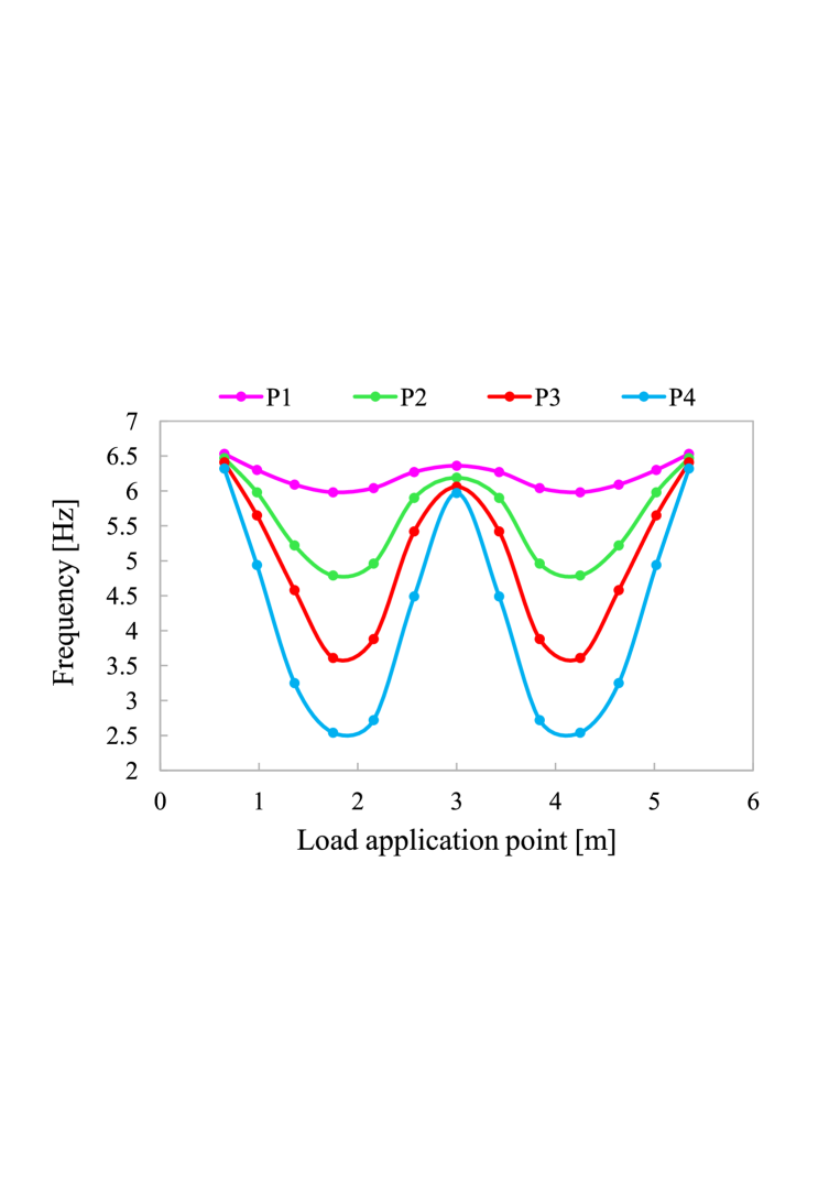
Figure 6: The structure’s frequency $\text{f}_{\text{1}}$ vs. the position of the concentrated load P for different load increments.

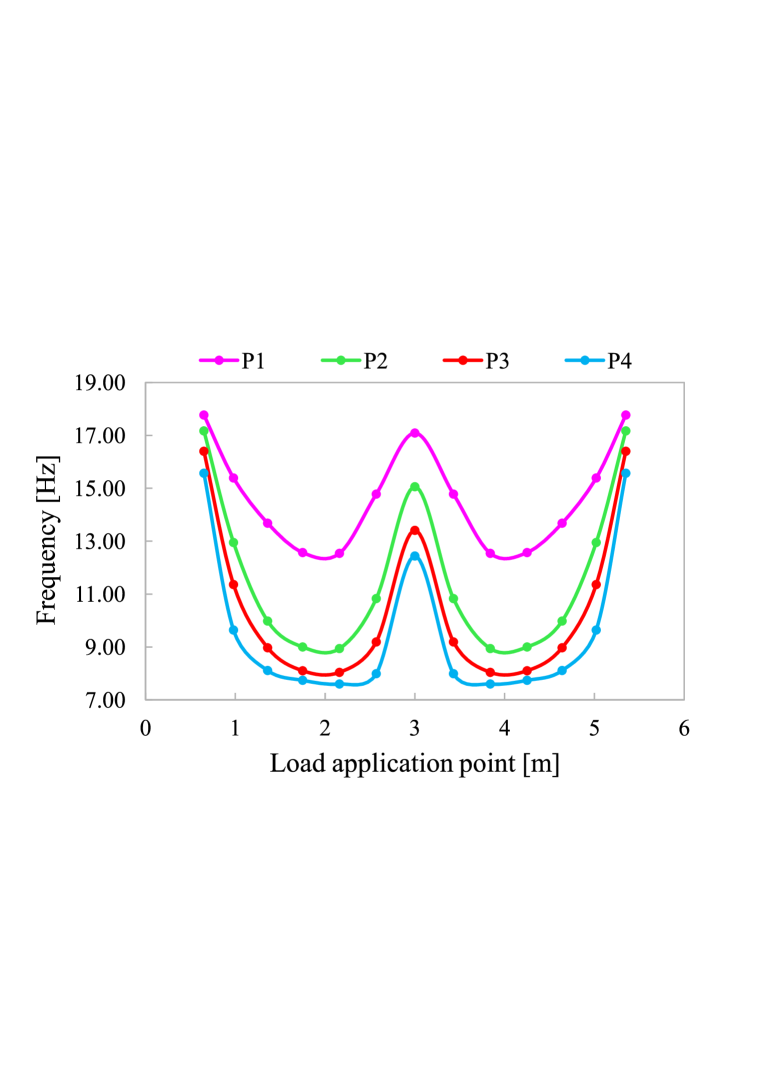
Figure 7: The structure’s frequency $\text{f}_{\text{2}}$ vs. the position of the concentrated load P for different load increments.

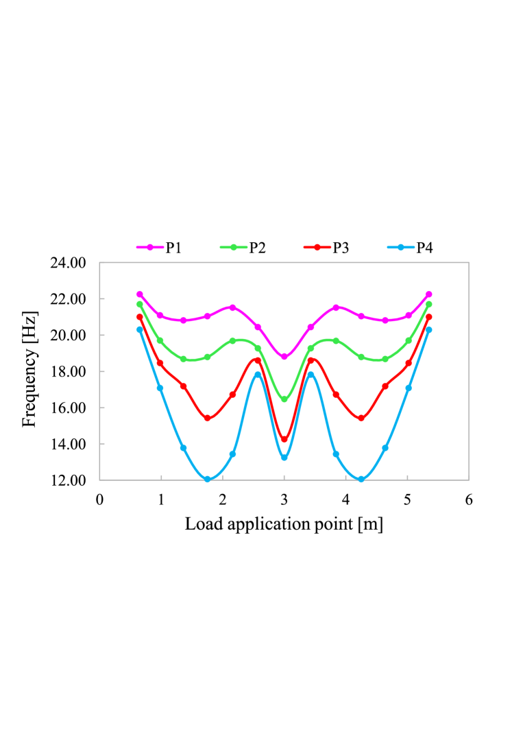
Figure 8: The structure’s frequency $\text{f}_{\text{3}}$ vs. the position of the concentrated load P for different load increments.

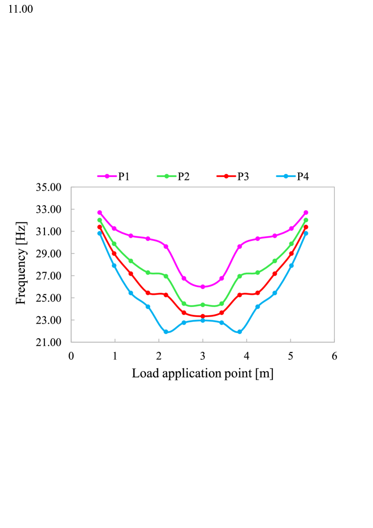
Figure 9: The structure’s frequency $\text{f}_{\text{4}}$ vs. the position of the concentrated load P for different load increments.

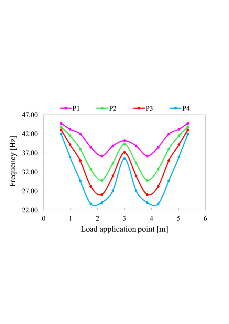
Figure 10: The structure’s frequency $\text{f}_{\text{5}}$ vs. the position of the concentrated load P for different load increments.

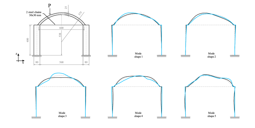
Figure 11: The first five mode shapes of the structure for load P at position $X_{4}$: linear elastic (black) and masonry–like (cyan) case. The masonry–like case is shown for the last load increment (length in cm).

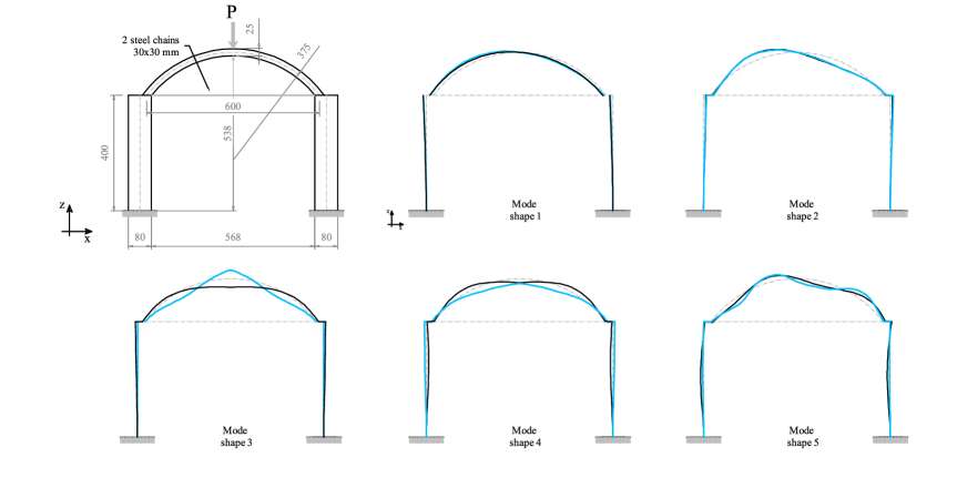
Figure 12: The first five mode shapes of the structure for load P at position $X_{7}$: linear elastic (black) and masonry–like (cyan) case. The masonry–like case is shown for the last load increment.

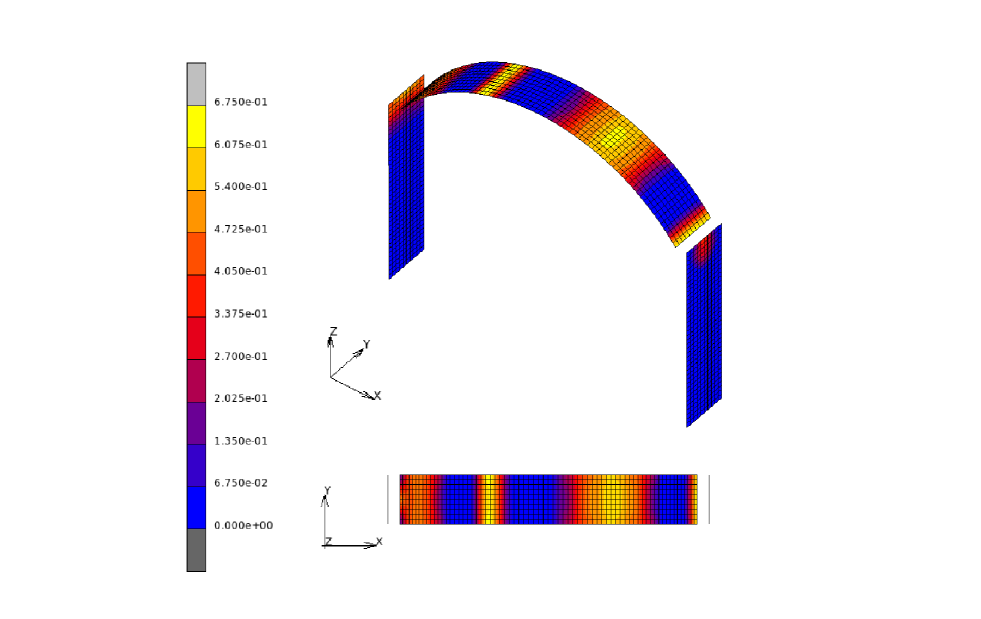
Figure 13: Distribution of $d_{e}$, $e=1,..,1500$ in the structure for the load P at position $X_{4}$. The result refers to the last load increment.

Figure 14: Distribution of $d_{e}$, $e=1,..,1500$ in the structure for the load P at position $X_{7}$. The result refers to the last load increment.

Figure 15: Fracture strain $E_{22}^{f}$ at the intrados (left) and the extrados (right) of the structure for load P at position $X_{4}$.

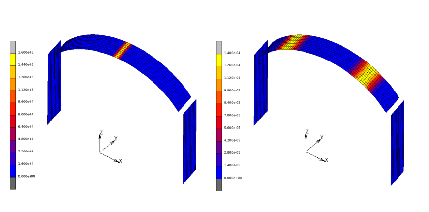
Figure 16: Fracture strain $E_{22}^{f}$ at the intrados (left) and the extrados (right) of the structure for load P at position $X_{7}$.

4.3 The bell tower of the Church of San Frediano in Lucca

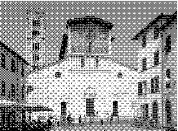
Figure 17: The Basilica of San Frediano in Lucca (Italy). On the left, the San Frediano bell tower.

The Basilica of San Frediano (Figure 17), dating back to the 11th century, is one of the most fascinating monuments in Lucca, much of its fascination being due to the marvellous mosaics that adorn its façade. In June 2015 the church’s 52 m high bell tower was fitted with four high–sensitivity triaxial seismometric stations, made available by the Arezzo Earthquake Observatory (Osservatorio Sismologico di Arezzo) and left active on the tower for three days (Figure 18). Data from the instruments, analyzed via OMA techniques [29], allowed us to determine the tower’s first five natural frequencies $f_{\text{i}}^{\text{exp}}$ and corresponding damping ratios [28]. Information on the mode shapes was also extracted, though the arrangement of the sensors, aligned along the vertical, did not allow for reliable identification of the torsional modes.

In the following the NOSA–ITACA code, together with model updating techniques, is employed in order to fit the experimental results in the linear elastic and the masonry–like (nonlinear) case. The finite–element model of the tower consists of $18495$ thick shell elements [36]. The four steel tie rods fitted to the masonry vault under the bell chamber (between section $3$ and section $4$ in Figure 18) are modelled with beam elements [23], which have also been used to model the wooden trusses and rafters constituting the pavillion roof covering the tower. The mechanical properties of the tie rods and wooden elements are, respectively, $E=2.1\cdot 10^{5}$ MPa, $\nu=0.3$, $\rho=$7850\text{\,}\mathrm{k}\mathrm{g}\mathrm{/}\mathrm{m}^{3}$$ and $E=9500$ MPa, $\nu=0.4$, $\rho=$800\text{\,}\mathrm{k}\mathrm{g}\mathrm{/}\mathrm{m}^{3}$$. With regard to the materials constituting the masonry tower, no experimental information is available to date. Visual inspection reveals that the external layers of the walls are made up of regular stone blocks at the base, while quite homogeneous brick masonry forms the upper part, except for the central part of the walls, where the masonry between the windows is made up of stone blocks. A first attempt to fit the experimental results through model updating procedures, conducted in [28], showed that good results can be achieved by assuming homogeneous values for the mechanical properties of all the materials making up the tower. Herein we proceed in the same way by assuming Young’s modulus $E$ and the mass density $\rho$ of masonry as parameters to be updated. In particular, for different values of $E$ and $\rho$ satisfying

$$$3\cdot 10^{9}\,\text{\,}\mathrm{Pa}$\leq E\leq$7\cdot 10^{9}\,\text{\,}\mathrm{Pa}$,$$

$$$1800\text{\,}\mathrm{k}\mathrm{g}\mathrm{/}\mathrm{m}^{3}$\leq\rho\leq$2200\text{\,}\mathrm{k}\mathrm{g}\mathrm{/}\mathrm{m}^{3}$,$$ (42)

the first five natural frequencies of the tower are calculated for the linear elastic and nonlinear case, after having applied the structure’s self–weight alone. The optimal values of $E$ and $\rho$, are determined by minimizing the functions

$$e^{l}(E,\rho)=\sum_{i=1}^{5}\left(f_{\text{i}}^{l}(E,\rho)-f_{\text{i}}^{\text{exp}}\right)^{2},$$ (43)

$$e(E,\rho)=\sum_{i=1}^{5}\left(f_{\text{i}}(E,\rho)-f_{\text{i}}^{\text{exp}}\right)^{2},$$ (44)

respectively in the linear and nonlinear cases, for $E$ and $\rho$ satisfying (42).

Figures 19 and 20 respectively show the functions $e^{l}$ and $e$ vs. $E$ and $\rho$. They reach their minimum values at $E=$4\cdot 10^{9}\,\text{\,}\mathrm{Pa}$$ and $\rho=$2000\text{\,}\mathrm{k}\mathrm{g}\mathrm{/}\mathrm{m}^{3}$$ for the linear elastic case and at $E=$5\cdot 10^{9}\,\text{\,}\mathrm{Pa}$$ and $\rho=$2000\text{\,}\mathrm{k}\mathrm{g}\mathrm{/}\mathrm{m}^{3}$$ for the nonlinear case. Figure 21 plots the two functions vs. $E$ for $\rho=$2000\text{\,}\mathrm{k}\mathrm{g}\mathrm{/}\mathrm{m}^{3}$$. The first five natural frequencies of the tower are shown in Table 7, where the experimental values $f_{\text{i}}^{\text{exp}}$ are compared with the numerical values, in the linear elastic $\left(f_{\text{i}}^{l}\right)$ and nonlinear $\left(f_{\text{i}}\right)$ case. Columns $\Delta f_{\text{i}}^{l}$ and $\Delta f_{\text{i}}$ show the differences between the numerical and experimental values for the linear and nonlinear case, respectively. The numerical frequencies differ from the experimental values by no more than five percent. The nonlinear case is more accurate in evaluating the higher modes. Figure 22 shows the first five mode shapes, calculated in the nonlinear case for the optimal values $\big{(}E=$5\cdot 10^{9}\,\text{\,}\mathrm{Pa}$,\,\rho=$2000\text{\,}\mathrm{k}\mathrm{g}\mathrm{/}\mathrm{m}^{3}$\big{)}$. They are substantially equal to the linear elastic modes, which are shown in [28]. The Figure clearly shows that the third mode is torsional. Finally, Figure 23 shows the maximum principal fracture strains for the tower in equilibrium with its own weight in the inner and outer layers of the mesh for $E=$5\cdot 10^{9}\,\text{\,}\mathrm{Pa}$$ and $\rho=$2000\text{\,}\mathrm{k}\mathrm{g}\mathrm{/}\mathrm{m}^{3}$$. The crack distribution and the low values of the fracture strains indicate a modest level of damage inside the structure: the fracture strains are concentrated around the windows and lintels, and in the masonry supporting the vault under the bell chamber. This confirms the observations made upon visual inspection. Crack strains are concentrated in regions of the structure quite far from those of the highest curvatures for the first mode shapes, which in fact remain very similar to those calculated in the linear elastic case. However, due to the nonlinearity of the constitutive equation adopted, the model updating procedure yields higher values of Young’s modulus, which increases by about the twenty–five percent with respect to the linear elastic case.

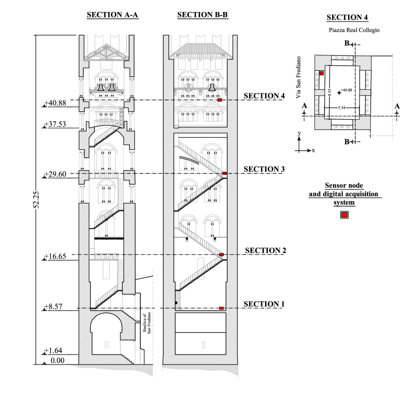
Figure 18: Sections of the San Frediano bell tower and sensors’ arrangement.

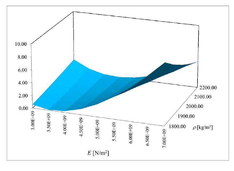
Figure 19: Function $e^{l}(E,\rho)$: linear case.

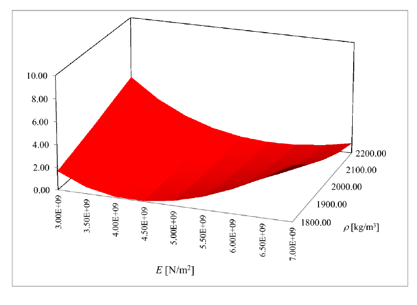
Figure 20: Function $e(E,\rho)$: nonlinear case.

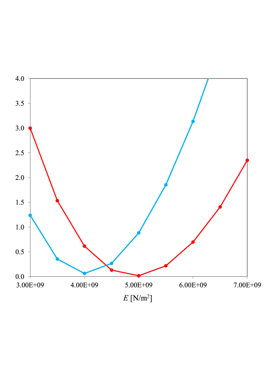
Figure 21: Functions $e(E,\rho)$ (red line) and $e^{l}(E,\rho)$ (blue line) vs. E for $\rho=$2000\text{\,}\mathrm{k}\mathrm{g}\mathrm{/}\mathrm{m}^{3}$$.

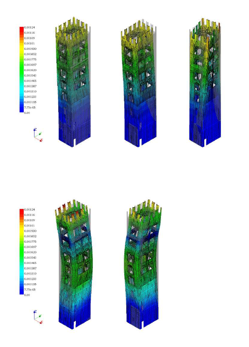
Figure 22: Mode shapes $\phi_{i}$, $i=1,..,5$ of the San Frediano bell tower in the nonlinear case, for $E=$5\cdot 10^{9}\,\text{\,}\mathrm{Pa}$,\,\rho=$2000\text{\,}\mathrm{k}\mathrm{g}\mathrm{/}\mathrm{m}^{3}$$.

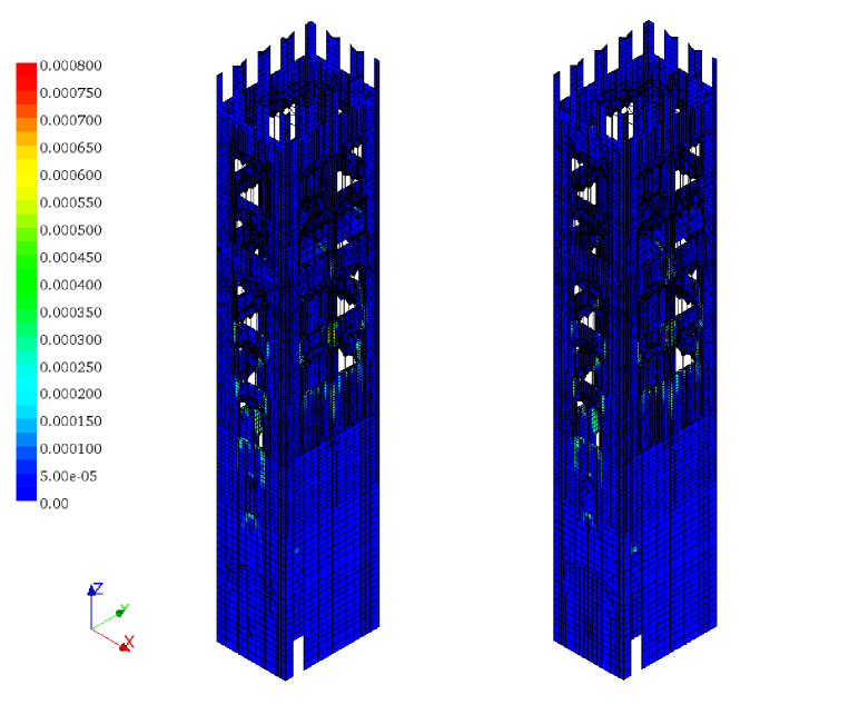
Figure 23: Maximum principal fracture strains in the San Frediano bell tower: inner (on the left) and outer (on the right) layers, for $E=$5\cdot 10^{9}\,\text{\,}\mathrm{Pa}$,\,\rho=$2000\text{\,}\mathrm{k}\mathrm{g}\mathrm{/}\mathrm{m}^{3}$$.

List of Figures

1. 1 The geometry of the beam (left) and its first six mode shapes (right): linear elastic (black) and masonry–like (cyan) case (lengths in cm). The masonry–like case is shown for the last load increment.
2. 2 The ratio $\text{f}_{\text{i}}/{\text{f}_{\text{i}}}^{l}$ for the first six natural frequencies of the beam vs. the lateral load.
3. 3 The quantities MAC–$M(\phi_{3}^{l},\phi_{3})$ (blue line) and MAC–$M(\phi_{3}^{l},\phi_{4})$ (green line) vs. the lateral load.
4. 4 The ratio between the cracked area $\text{A}_{\text{f}}$ and total area A along the beam at the last load increment. (lengths in cm).
5. 5 Geometry of the structure made of up the arch on piers and the different positions along the arch span at which the concentrated load P is applied (length in cm). The local axes of the finite–elements are drawn in red.
6. 6 The structure’s frequency $\text{f}_{\text{1}}$ vs. the position of the concentrated load P for different load increments.
7. 7 The structure’s frequency $\text{f}_{\text{2}}$ vs. the position of the concentrated load P for different load increments.
8. 8 The structure’s frequency $\text{f}_{\text{3}}$ vs. the position of the concentrated load P for different load increments.
9. 9 The structure’s frequency $\text{f}_{\text{4}}$ vs. the position of the concentrated load P for different load increments.
10. 10 The structure’s frequency $\text{f}_{\text{5}}$ vs. the position of the concentrated load P for different load increments.
11. 11 The first five mode shapes of the structure for load P at position $X_{4}$: linear elastic (black) and masonry–like (cyan) case. The masonry–like case is shown for the last load increment (length in cm).
12. 12 The first five mode shapes of the structure for load P at position $X_{7}$: linear elastic (black) and masonry–like (cyan) case. The masonry–like case is shown for the last load increment.
13. 13 Distribution of $d_{e}$, $e=1,..,1500$ in the structure for the load P at position $X_{4}$. The result refers to the last load increment.
14. 14 Distribution of $d_{e}$, $e=1,..,1500$ in the structure for the load P at position $X_{7}$. The result refers to the last load increment.
15. 15 Fracture strain $E_{22}^{f}$ at the intrados (left) and the extrados (right) of the structure for load P at position $X_{4}$.
16. 16 Fracture strain $E_{22}^{f}$ at the intrados (left) and the extrados (right) of the structure for load P at position $X_{7}$.
17. 17 The Basilica of San Frediano in Lucca (Italy). On the left, the San Frediano bell tower.
18. 18 Sections of the San Frediano bell tower and sensors’ arrangement.
19. 19 Function $e^{l}(E,\rho)$: linear case.
20. 20 Function $e(E,\rho)$: nonlinear case.
21. 21 Functions $e(E,\rho)$ (red line) and $e^{l}(E,\rho)$ (blue line) vs. E for $\rho=$2000\text{\,}\mathrm{k}\mathrm{g}\mathrm{/}\mathrm{m}^{3}$$.
22. 22 Mode shapes $\phi_{i}$, $i=1,..,5$ of the San Frediano bell tower in the nonlinear case, for $E=$5\cdot 10^{9}\,\text{\,}\mathrm{Pa}$,\,\rho=$2000\text{\,}\mathrm{k}\mathrm{g}\mathrm{/}\mathrm{m}^{3}$$.
23. 23 Maximum principal fracture strains in the San Frediano bell tower: inner (on the left) and outer (on the right) layers, for $E=$5\cdot 10^{9}\,\text{\,}\mathrm{Pa}$,\,\rho=$2000\text{\,}\mathrm{k}\mathrm{g}\mathrm{/}\mathrm{m}^{3}$$.

5 Conclusions

The paper deals with the modal analysis of masonry structures. In particular, a new procedure for calculating the natural frequencies and mode shapes of masonry buildings has been implemented within the NOSA–ITACA code, to take into account the inability of masonry to withstand tensile stresses. Some structures have been analyzed and the influence on their dynamic properties of the fracture strains induced by their self-weights and external loads investigated. In particular, the new algorithm has been applied to the finite–element model of the San Frediano bell tower in Lucca, and the results of the numerical simulation compared with those from an experimental campaign conducted on the tower in June, 2015. The new procedure provides for more realistic simulations of the dynamic behaviour of masonry structures in the presence of cracks and, when combined with experimental data, can be helpful in assessing damage. Moreover, the dependence of the natural frequencies on external loads (the case of thermal loads is under development) can be assessed, and used to interpret data from long–term monitoring protocols.

$\begin{array}[]{c}\text{Lateral}\\ \text{load [N]}\end{array}$	$\textbf{f}_{\mathbf{1}}[\mathrm{Hz}]$	$\begin{array}[]{c}\text{Eff. modal}\\ \text{mass [\%]}\end{array}$		$\textbf{f}_{\mathbf{2}}[\mathrm{Hz}]$	$\begin{array}[]{c}\text{Eff. modal}\\ \text{mass [\%]}\end{array}$		$\textbf{f}_{\mathbf{3}}[\mathrm{Hz}]$	$\begin{array}[]{c}\text{Eff. modal}\\ \text{mass [\%]}\end{array}$
		y	z		y	z		y	z
0	6.47	80.73	0.00	25.48	0.00	0.00	53.79	0.00	81.06
9000	6.44	80.73	0.00	25.48	0.00	0.00	53.74	0.00	80.76
10125	6.13	80.32	0.00	25.27	0.00	0.00	52.63	2.95	54.97
11250	5.74	79.98	0.00	24.36	0.00	0.00	51.22	4.42	44.12
12375	5.23	79.53	0.00	23.12	0.00	0.00	48.97	6.05	32.33
13500	4.72	79.09	0.00	21.80	0.00	0.00	46.14	7.38	22.13
14625	4.21	78.77	0.00	19.95	0.00	0.00	43.75	8.10	16.40
15750	3.71	78.35	0.00	18.34	0.00	0.00	40.69	8.60	12.06

$\begin{array}[]{c}\text{Lateral}\\ \text{load }$[N]$\end{array}$	$\textbf{f}_{\mathbf{4}}[\mathrm{Hz}]$	$\begin{array}[]{c}\text{Eff. modal}\\ \text{mass [\%]}\end{array}$		$\textbf{f}_{\mathbf{5}}[\mathrm{Hz}]$	$\begin{array}[]{c}\text{Eff. modal}\\ \text{mass [\%]}\end{array}$		$\textbf{f}_{\mathbf{6}}[\mathrm{Hz}]$	$\begin{array}[]{c}\text{Eff. modal}\\ \text{mass [\%]}\end{array}$
		y	z		y	z		y	z
0	55.96	8.77	0.00	96.43	0.00	0.00	145.30	3.07	0.00
9000	55.71	8.77	0.00	96.37	0.00	0.00	144.79	3.07	0.00
10125	54.69	6.15	25.67	94.51	0.00	0.00	141.80	3.10	0.00
11250	54.30	4.90	36.06	90.15	0.00	0.00	137.51	3.11	0.00
12375	53.46	3.41	47.18	85.85	0.00	0.00	130.80	3.27	0.00
13500	52.31	2.07	56.67	82.42	0.00	0.00	122.50	3.49	0.00
14625	50.79	1.22	61.54	76.97	0.00	0.00	115.60	3.72	0.00
15750	49.37	0.06	64.93	71.94	0.00	0.00	108.10	3.92	0.00

Table 1: The beam’s natural frequencies $\text{f}_{\text{i}}$, $i=1,...,6$ and the effective modal masses of the corresponding mode shapes versus load increments.

MAC – $M$
	$\phi_{1}$	$\phi_{2}$	$\phi_{3}$	$\phi_{4}$	$\phi_{5}$	$\phi_{6}$
$\phi_{1}^{l}$	0.99	0.00	0.06	0.03	0.00	0.00
$\phi_{2}^{l}$	0.00	0.99	0.02	0.04	0.12	0.00
$\phi_{3}^{l}$	0.05	0.04	0.41	0.90	0.04	0.01
$\phi_{4}^{l}$	0.04	0.00	0.88	0.41	0.01	0.19
$\phi_{5}^{l}$	0.00	0.12	0.00	0.04	0.95	0.00
$\phi_{6}^{l}$	0.00	0.00	0.16	0.09	0.00	0.93

Table 2: MAC–$M(\phi_{\text{i}}^{l},\phi_{\text{j}})$, for i,j = 1, 2, …, 6 at the last load increment.

$\begin{array}[]{c}\text{Total}\\ \text{vertical}\\ \text{load }[N]\end{array}$	$\textbf{f}_{\mathbf{1}}[\mathrm{Hz}]$	$\begin{array}[]{c}\text{Eff. modal}\\ \text{mass [\%]}\end{array}$		$\textbf{f}_{\mathbf{2}}[\mathrm{Hz}]$	$\begin{array}[]{c}\text{Eff. modal}\\ \text{mass [\%]}\end{array}$		$\textbf{f}_{\mathbf{3}}[\mathrm{Hz}]$	$\begin{array}[]{c}\text{Eff. modal}\\ \text{mass [\%]}\end{array}$
		x	z		x	z		x	z
0	6.54	59.43	0.00	18.81	8.75	0.00	22.49	0.00	7.92
144605	6.53	59.29	0.00	18.50	8.83	0.00	22.01	0.00	6.98
$\text{P}_{1}$=150605	5.98	51.21	0.00	12.57	15.47	0.00	21.04	0.00	5.91
$\text{P}_{2}$=152605	4.79	28.54	0.00	9.00	37.27	0.00	18.79	0.00	2.92
$\text{P}_{3}$=153605	3.61	15.38	0.00	8.10	50.00	0.00	15.43	0.00	0.92
$\text{P}_{4}$=154605	2.54	9.91	1.32	7.74	77.4	0.00	12.06	0.00	0.30

$\begin{array}[]{c}\text{Total}\\ \text{vertical}\\ \text{load }[N]\end{array}$	$\textbf{f}_{\mathbf{4}}[\mathrm{Hz}]$	$\begin{array}[]{c}\text{Eff. modal}\\ \text{mass [\%]}\end{array}$		$\textbf{f}_{\mathbf{5}}[\mathrm{Hz}]$	$\begin{array}[]{c}\text{Eff. modal}\\ \text{mass [\%]}\end{array}$
		x	z		x	z
0	33.74	0.00	1.57	45.37	11.88	0.00
144605	32.44	0.00	2.82	44.80	11.28	0.00
$\text{P}_{1}$=150605	30.34	0.00	4.55	38.48	6.74	0.00
$\text{P}_{2}$=152605	27.28	0.00	8.91	32.70	3.96	0.00
$\text{P}_{3}$=153605	25.45	0.00	11.08	28.19	2.98	0.00
$\text{P}_{4}$=154605	24.20	0.00	11.70	23.60	1.39	0.00

Table 3: The structure’s natural frequencies $\text{f}_{\text{i}}$, $i=1,..,5$ and the effective modal masses of the corresponding mode shapes versus load increments. Load P at position $X_{4}$.

MAC – $M$
	$\phi_{1}$	$\phi_{2}$	$\phi_{3}$	$\phi_{4}$	$\phi_{5}$
$\phi_{1}^{l}$	0.64	0.77	0.00	0.00	0.00
$\phi_{2}^{l}$	0.71	0.59	0.05	0.08	0.31
$\phi_{3}^{l}$	0.14	0.11	0.68	0.43	0.56
$\phi_{4}^{l}$	0.07	0.06	0.52	0.63	0.07
$\phi_{5}^{l}$	0.10	0.09	0.19	0.17	0.57

Table 4: MAC–$M(\phi_{\text{i}}^{l},\phi_{\text{j}})$, for i,j = 1, 2, …, 5 at the last load increment. Load P at position $X_{4}$.

$\begin{array}[]{c}\text{Total}\\ \text{vertical}\\ \text{load }[N]\end{array}$	$\textbf{f}_{\mathbf{1}}[\mathrm{Hz}]$	$\begin{array}[]{c}\text{Eff. modal}\\ \text{mass [\%]}\end{array}$		$\textbf{f}_{\mathbf{2}}[\mathrm{Hz}]$	$\begin{array}[]{c}\text{Eff. modal}\\ \text{mass [\%]}\end{array}$		$\textbf{f}_{\mathbf{3}}[\mathrm{Hz}]$	$\begin{array}[]{c}\text{Eff. modal}\\ \text{mass [\%]}\end{array}$
		x	z		x	z		x	z
0	6.54	59.43	0.00	18.81	8.75	0.00	22.49	0.00	7.92
144605	6.53	59.29	0.00	18.50	8.83	0.00	22.01	0.00	6.98
$\text{P}_{1}$=150605	6.36	57.80	0.00	17.09	9.99	0.00	18.82	0.00	0.70
$\text{P}_{2}$=152605	6.19	55.55	0.00	15.06	11.89	0.00	16.47	0.00	0.00
$\text{P}_{3}$=153605	6.06	53.07	0.00	13.41	14.08	0.00	14.26	0.00	0.60
$\text{P}_{4}$=154605	5.97	51.06	0.00	12.44	15.92	0.00	13.25	0.00	0.10

$\begin{array}[]{c}\text{Total}\\ \text{vertical}\\ \text{load }[N]\end{array}$	$\textbf{f}_{\mathbf{4}}[\mathrm{Hz}]$	$\begin{array}[]{c}\text{Eff. modal}\\ \text{mass [\%]}\end{array}$		$\textbf{f}_{\mathbf{5}}[\mathrm{Hz}]$	$\begin{array}[]{c}\text{Eff. modal}\\ \text{mass [\%]}\end{array}$
		x	z		x	z
0	33.74	0.00	1.57	45.37	11.88	0.00
144605	32.44	0.00	2.82	44.80	11.28	0.00
$\text{P}_{1}$=150605	26.00	0.00	12.76	40.18	0.00	5.55
$\text{P}_{2}$=152605	24.37	0.00	14.06	39.31	0.00	3.69
$\text{P}_{3}$=153605	23.34	0.00	13.78	37.13	2.74	0.00
$\text{P}_{4}$=154605	22.96	0.00	13.41	35.52	2.09	0.00

Table 5: The structure’s natural frequencies $\text{f}_{\text{i}}$, $i=1,..,5$, and the effective modal masses of the corresponding mode shapes versus load increments. Load P at position $X_{7}$.

MAC – $M$
	$\phi_{1}$	$\phi_{2}$	$\phi_{3}$	$\phi_{4}$	$\phi_{5}$
$\phi_{1}^{l}$	0.98	0.17	0.00	0.00	0.00
$\phi_{2}^{l}$	0.17	0.98	0.00	0.00	0.04
$\phi_{3}^{l}$	0.00	0.00	0.46	0.89	0.00
$\phi_{4}^{l}$	0.00	0.00	0.64	0.34	0.00
$\phi_{5}^{l}$	0.00	0.03	0.00	0.00	0.75

Table 6: MAC–$M(\phi_{\text{i}}^{l},\phi_{\text{j}})$, for i,j = 1, 2, …, 5 at the last load increment. Load P at position $X_{7}$.

	$f_{\text{i}}^{\text{exp}}$	$f_{\text{i}}^{l}$	$\Delta f_{\text{i}}^{l}$	$f_{\text{i}}$	$\Delta f_{\text{i}}$
Mode Shape 1	1.14	1.15	0.01	1.18	0.04
Mode Shape 2	1.38	1.38	0.00	1.41	0.02
Mode Shape 3	3.44	3.60	0.05	3.39	-0.01
Mode Shape 4	4.60	4.41	-0.04	4.61	0.00
Mode Shape 5	5.34	5.35	0.00	5.44	0.02

Table 7: Natural frequencies [Hz] of the tower: experimental values $f_{\text{i}}^{\text{exp}}$, numerical values $f_{\text{i}}^{l}$ identified on the linear elastic model; numerical values $f_{\text{i}}$ identified on the masonry–like model.

References

- [1] Dimarogonas AD. Vibration of cracked structures: a state of art review. Engineering Fracture Mechanics 1996; 55(5):831-857, Elsevier.
- [2] Salawu OS. Detection of structural damage through changes in frequency: a review. Engineering Structures 1997; 19(9): 718–723, Elsevier.
- [3] Dos Santos FLM, Peeters B, Van der Auweraer H, Goes LCS, Desmet W. Vibration-based damage detection for a composite helicopter main rotor blade. Case Studies in Mechanical Systems and Signal Processing 2016; http://dx.doi.org/10.1016/j.csmssp.2016.01.001.
- [4] Agarwali S, Chaudhuri SR. Damage detection in large structures using mode shapes and its derivatives. International Journal of Research in Engineering and Technology 2015; 4, Special Issue 13.
- [5] Wahab MMA. Effect of modal curvatures on damage detection using model updating. Mechanical Systems and Signal Processing 2001; 15(2): 439–445, Elsevier.
- [6] Azzara RM, Zaccarelli L, Morelli A, Trombetti T, Dallavalle G, Cavaliere A, Danesi S. Seismic monitoring of the Asinelli and Garisenda medioeval towers in Bologna (Italy), an instrumental contribution to the engineering modeling direct to their protection. Proceedings of the second International Conference on Protection of Historical Constructions 2014; F. M. Mazzolani and G. Altay (Eds), Bogaziçi University Publishing.
- [7] Gentile C, Saisi A, Cabboi A, Dynamic monitoring of a masonry tower. Proceedings of the 8th International Conference on Structural Analysis of Historical Constructions, SAHC 2012 2012; Jasienko J. (Ed).
- [8] Ramos LF , Marques L , Lourenço PB , De Roeck G, Campos-Costa A, Roque J. Monitoring historical masonry structures with operational modal analysis: two cas studies. Mech. Syst. Signal Process 2010; 24: 1291-1305, Elsevier.
- [9] Abbiati G, Ceravolo R, Surace C. Time-dependent estimators for on-line monitoring of full-scale structures under ambient excitation. Mechanical Systems and Signal Processing 2015; 60–61: 166–181.
- [10] Ramos LF, De Roeck G, Lourenço PB, Campos–Costa A. Damage identification on arched masonry structures using ambient and random impact vibrations. Engineering Structures 2010; 32: 146–162, Elsevier.
- [11] Gentile C, Saisi A. Operational modal testing of historic structures at different levels of excitation. Construction and buiding Materials 2013; 48:1273–1285.
- [12] Saisi A, Gentile C, Guidobaldi M. Post–earthquanke continuous dynamic monitoring of the Gabbia Tower in Mantua, Italy. Construction and Buiding Materials 2015; 48:1273–1285, Elsevier.
- [13] Ren WX, De Roeck G. Structural Damage Identification using Modal Data. I: Simulation Verification. Journal of Structural Engineering 2002; 128(1): 87–95, ASCE.
- [14] Ren WX, De Roeck G. Structural Damage Identification using Modal Data. II: Test Verification. Journal of Structural Engineering 2002; 128(1): 96–104, ASCE.
- [15] Jayanthan M, Srinivas V. Structural Damage Identification Based on Finite Element Model Updating. Journal of Mechanical Engineering and Automation 2015; 5(3B): 59-63.
- [16] Pineda P. Collapse and upgrading mechanisms associated to the structural materials of a deteriorated masonry tower. Nonlinear assessment under different damage and loading levels. Engineering Failure Analysis 2016; 63:72–93, Elsevier.
- [17] Bui TT, Limam A, Bui QB. Characterisation of vibration and damage in masonry structures: experimental and numerical analysis. European Journal of Environmental and Civil Engineering 2014; 18(10), 1118–1129.
- [18] Cakti E, Saygili O, Lemos JV, Oliveira CS. A parametric study of the earthquake behaviour of masonry minarets. Proceedings of the Tenth U.S. National Conference on Earthquake Engineering Frontiers of Earthquake Engineering, 10NCEE, 2014. July 21-25, Anchorage, Alaska.
- [19] Girardi M, Lucchesi M. Free flexural vibrations of masonry beam–columns. Journal of Mechanics of Materials and Structures 2010; 5(1): 143–159.
- [20] Del Piero G. Constitutive equations and compatibility of external loads for linear elastic masonry–like materials. Meccanica 1989; 24:150–162.
- [21] Di Pasquale S. New trends in the analysis of masonry structures. Meccanica, 1992. 27:173–184.
- [22] Lucchesi M, Padovani C, Pasquinelli G, Zani N. Masonry constructions: mechanical models and numerical applications 2008; Lecture Notes in Applied and Computational Mechanics. Springer–Verlag.
- [23] Binante V, Girardi M, Padovani C, Pasquinelli G, Pellegrini D, Porcelli M. NOSA-ITACA 1.0 documentation 2014. www.nosaitaca.it/en.
- [24] http://www.nosaitaca.it
- [25] Harak SS, Sharma SC, Harsha SP. Modal analysis of prestressed draft pad of freight wagons using finite element method. J. Mod. Transport 2015; 23(1):43–49.
- [26] Noble D, Nogal M, O’Connor AJ, Pakrashi V. The effect of post-tensioning force magnitude and eccentricity on the natural bending frequency of cracked post-tensioned concrete beams, Journal of Physics. Conference Series 628, 2015. IOPscience.
- [27] Porcelli M, Binante V, Girardi M, Padovani C, Pasquinelli G. A solution procedure for constrained eigenvalue problems and its application within the structural finite-element code NOSA–ITACA. Calcolo 2015; 52(2): 167–186, Springer Milan.
- [28] Azzara RM, De Roeck G, Girardi M, Padovani C, Pellegrini D, Reynder E. Assessment of the dynamic behaviour of an ancient masonry tower in Lucca via ambient vibrations. Structural Analysis of Historical Constructions–Anamnesis, diagnosis, therapy, controls 2016; Van Balen and Verstrynge (Eds), ISBN 978–1–138–02951–4.
- [29] Brincker R, Ventura C. Introduction to Operational Modal Analysis 2015. John Wiley & Sons.
- [30] Padovani C, Silhavy M. On the derivative of the stress-strain relation in a no-tension material. Mathematics and Mechanics of Solids 2015; Online First 27 February 2015, Sage Publications Inc.
- [31] Degl’Innocenti S, Padovani C, Pasquinelli G. Numerical methods for the dynamic analysis of masonry structures. Structural Engineering and Mechanics 2006; 22(1): 107-130.
- [32] Bathe KJ, Wilson EL. Numerical Methods in Finite Element Analysis 1976. Prentice-Hall.
- [33] Lucchesi M, Padovani C, Pasquinelli G, Zani N. Static analysis of masonry vaults, constitutive model and numerical analysis. Journal of Mechanics of Materials and Structures 2007; 2(2), 221–224. Mathematical Science Publishers.
- [34] Bernardeschi K, Padovani C, Pasquinelli G. Numerical modelling of the structural behaviour of Buti’s bell tower. Journal of Cultural Heritage 2004; 5(4): 371–378.
- [35] http://www.salome-platform.org
- [36] Girardi M, Padovani C, Pellegrini D. The NOSA-ITACA code for the safety assessment of ancient constructions: a case study in Livorno. Advances in Engineering Software 2015. 89, 64–76.
- [37] D.M. 14 gennaio 2008, Norme Tecniche per le Costruzioni, G.U. 4 febbraio 2008, n. 29.
- [38] Saad Y. Iterative methods for sparse linear systems 2003. (2nd edition), SIAM.
- [39] Lehoucq RB, Sorensen DC, Yang C. ARPACK Users Guide. Solution of Large Scale Eigenvalue Problem with Implicit Restarted Arnoldi Methods 1998. SIAM.
- [40] Gurtin ME. The linear theory of elasticity. Encyclopedia of Physics, Vol. VIa/2, Mechanics of Solids II 1972. Truesdell C. (Ed). Springer-Verlag.
- [41] Clough RW, Penzien J. Dynamics of Structures 1975. McGraw–Hill Inc.
- [42] Nayfeh AH. Nonlinear Interactions 2000. Wiley Series in Nonlinear Science. John Wiley & Sons Inc.
- [43] Karnovsky IA. Theory of Arched Structures. Springer Science + Business Media, ISBN 978-1-4614-0468-2.