On the Convergence of the EM Algorithm:
A Data-Adaptive Analysis

Abstract

The Expectation-Maximization (EM) algorithm is an iterative method to maximize the log-likelihood function for parameter estimation. Previous works on the convergence analysis of the EM algorithm have established results on the asymptotic (population level) convergence rate of the algorithm. In this paper, we give a data-adaptive analysis of the sample level local convergence rate of the EM algorithm. In particular, we show that the local convergence rate of the EM algorithm is a random variable $\overline{K}_{n}$ derived from the data generating distribution, which adaptively yields the convergence rate of the EM algorithm on each finite sample data set from the same population distribution. We then give a non-asymptotic concentration bound of $\overline{K}_{n}$ on the population level optimal convergence rate $\overline{\kappa}$ of the EM algorithm, which implies that $\overline{K}_{n}\to\overline{\kappa}$ in probability as the sample size $n\to\infty$. Our theory identifies the effect of sample size on the convergence behavior of sample EM sequence, and explains a surprising phenomenon in applications of the EM algorithm, i.e. the finite sample version of the algorithm sometimes converges faster even than the population version. We apply our theory to the EM algorithm on three canonical models and obtain specific forms of the adaptive convergence theorem for each model.

1 Introduction

The iterative algorithm of expectation-maximization (EM) has been proposed in various special forms by a number of authors as early as in the 1970s, notably [2, 24, 30, 29, 31, 32]. Since the advent of its modern formulation by Dempster, Laird and Rubin [12], the EM algorithm has received much attention in the statistical community. A vast literature on theoretical properties and real applications of the EM algorithm has been accumulated thereafter (see e.g. [12, 5, 40, 28, 22, 23]). Classical work of Wu [40] established general convergence results for EM sequences to the MLE or some stationary points of the log-likelihood function; Redner and Walker [28] proved asymptotic results on the convergence of the EM algorithm for mixture of densities from the exponential family; Meng and Rubin [22] analyzed both asymptotic componentwise and global convergence rates of the EM algorithm; some variants or generalizations of the EM algorithm were also proposed: Meng and Rubin [21] developed ECM algorithm to replace a complicated $M$-step by several simpler $CM$-steps (conditional maximization); Liu et al. [19] proposed PX-EM to use the expanded complete-data model to accelerate the convergence of the EM algorithm. The book of McLachlan and Krishnan [20] gave a comprehensive account on both theoretical and practical aspects of the EM algorithm.

Recent work of Balakrishnan et al. [1] presented statistical guarantees for the local linear convergence of the EM algorithm and first-order EM algorithm to the true population parameter $\theta^{*}$ within statistical precision. Along this line, Wang et al. [39] considered extensions to high-dimensional settings by introducing a truncation step; Yi and Caramanis [41] proved statistical guarantees for generalizations to regularized EM algorithms in high-dimensional latent variable models. In this paper, we give a data-adaptive analysis of the finite sample level convergence behavior of the EM algorithm, especially the dynamics of the convergence rate when the EM algorithm is performed on multiple finite random data sets (with possibly different sample sizes) sampled from the same population distribution.

1.1 Problem Setup

Suppose $\{\mathbb{P}_{\theta}\mid\theta\in\Omega\subseteq\mathbb{R}^{p}\}$ is a family of parametric distributions, and $\mathbb{P}_{\theta}$ has density function $p_{\theta}(y)$ with respect to the Lebesgue measure on $\mathbb{R}^{d}$. A set of i.i.d. samples $\{y_{k}\}_{k=1}^{n}$ of $Y\sim\mathbb{P}_{\theta^{*}}$ is observed, where $\theta^{*}\in\Omega$ is an unknown population true parameter.

In latent variable models, $Y$ is the observed part of a pair $(Y,Z)$ of random variables and $Z$ is a latent variable. Suppose $f_{\theta}(y,z)$ is the joint density of $(Y,Z)$ and for $\theta\in\Omega$, the density $p_{\theta}(y)=\int_{\mathcal{Z}}f_{\theta}(y,z)dz$ is the marginalization of $f_{\theta}(y,z)$ over $z$, then the EM algorithm can be applied to estimate $\theta^{*}$ from the samples $\{y_{k}\}_{k=1}^{n}$ of $Y\sim\mathbb{P}_{\theta^{*}}$.

Specifically, one first calculates the sample $Q$-function (see Definition 1 in [1]) by a conditional Expectation ($E$-step):

$$Q_{n}(\theta^{\prime}|\theta;\{y_{k}\})=\frac{1}{n}\sum_{k=1}^{n}\int_{\mathcal{Z}(y_{k})}\log\left(f_{\theta^{\prime}}(y_{k},z)\right)k_{\theta}(z|y_{k})dz,$$

where $k_{\theta}(z|y)\coloneqq\frac{f_{\theta}(y,z)}{p_{\theta}(y)}$ is the conditional density of $Z$ given $Y$. Then for an initial point $\theta_{n}^{0}\in B_{r}(\theta^{*})$, the sample EM sequence $\{\theta_{n}^{t}\}_{t\geq 0}$ is constructed by Maximization ($M$-step):

$$\theta_{n}^{t+1}\in\arg\max\{Q_{n}(\theta^{\prime}|\theta_{n}^{t};\{y_{k}\})\mid\theta^{\prime}\in\Omega\},$$

and we refer to this procedure as the EM algorithm is performed on the samples $\{y_{k}\}_{k=1}^{n}$.

We notice that the sample $Q$-function $Q_{n}(\theta^{\prime}|\theta;\{y_{k}\})$ depends on a specific set of samples $\{y_{k}\}_{k=1}^{n}$, hence so does the sample EM sequence $\{\theta_{n}^{t}\}_{t\geq 0}$ defined above. Since the samples are i.i.d. realizations of $Y\sim\mathbb{P}_{\theta^{*}}$, it is sensible to conjecture that the convergence rate of the sample EM sequence depends on the data generating distribution $\mathbb{P}_{\theta^{*}}$. When the EM algorithm is performed on different sets of samples from the same population, the corresponding sample EM sequences constructed as in the above procedure ought to converge at different rates. In the subsequent numerical experiments, we have also confirmed this phenomenon, e.g. see Figure 1. This observation motivates us to characterize the convergence rate of the EM algorithm as a data-adaptive quantity.

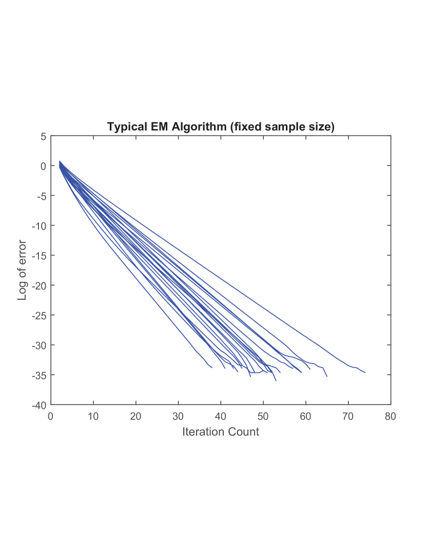
(a)

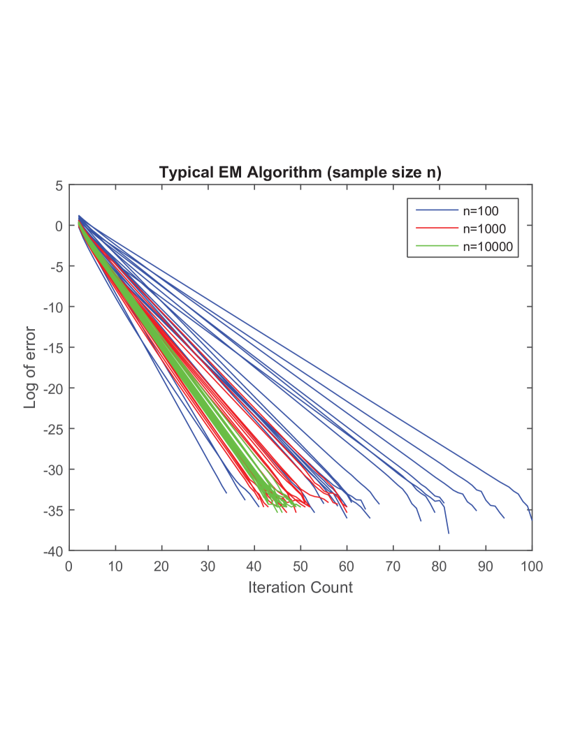
(b)

Figure 1: These plots are generated by applying the EM algorithm to simulated data from a fixed Gaussian Mixture Model (Section 4.1) with the dimension of $\theta^{*}$ set to $p=5$, and the SNR (Signal-to-Noise Ratio) $\frac{\left\|\theta^{*}\right\|}{\sigma}=1$. Each line in the plots represents an instance of the EM algorithm performed on a different data set sampled from the Gaussian mixture distribution; the convergence rates of the EM algorithm are the slopes of these lines. (a) 20 instances of the EM algorithm each performed on a different set of $n=300$ random samples; the slopes of the lines vary from one instance to another. (b) 20 instances of the EM algorithm performed on different sets of $n$ random samples for each $n\in\{100,1000,10000\}$; when the sample size is small, the lines are more spread-out (blue lines), hence the fluctuations in the convergence rate are large; when the sample size is large, the lines are more clustered (red lines and green lines), hence the fluctuations in the convergence rate are small.

1.2 Main Results and Contributions

The main results of this paper are as follows: we characterize the convergence rate of the empirical EM sequence as a derived random variable $\overline{K}_{n}$ of the data generating distribution $\mathbb{P}_{\theta^{*}}$ in Theorem 3.2, then we give the concentration bound of $\overline{K}_{n}$ in Theorem 3.4.

Optimal Empirical Convergence Theorem

The primary goal of Theorem 3.2 is to show that the convergence rate of the EM algorithm is a random variable. To this end, we adopt a novel data-adaptive viewpoint in the finite sample level analysis by considering the samples as i.i.d. copies $\{Y_{k}\}_{k=1}^{n}$ of the random variable $Y\sim\mathbb{P}_{\theta^{*}}$ and exploiting the concentration of measure phenomenon to obtain non-asymptotic sample level convergence results.

The theorem states that if the EM algorithm is initialized as $\Theta_{n}^{0}\in B_{r}(\theta^{*})$ in the ball of population contraction (to be defined precisely), then with high probability, we have a convergence inequality in the form

$$\left\|\Theta_{n}^{t}-\theta^{*}\right\|\leq\left(\overline{K}_{n}\right)^{t}\left\|\Theta_{n}^{0}-\theta^{*}\right\|+\frac{\overline{E}_{n}}{\overline{V}_{n}-\overline{\Gamma}_{n}},$$ (1)

where $\{\Theta_{n}^{t}\}_{t\geq 0}$ is the empirical EM sequence, defined as

$$\Theta_{n}^{t+1}\in\arg\max\{Q_{n}(\Theta^{\prime}|\Theta_{n}^{t};\{Y_{k}\})\mid\Theta^{\prime}\in B_{R}(\theta^{*})\},$$

for a set of i.i.d. copies $\{Y_{k}\}_{k=1}^{n}$ of $Y\sim\mathbb{P}_{\theta^{*}}$. The quantities $\overline{\varGamma}_{n}$, $\overline{V}_{n}$, $\overline{E}_{n}$ and $\overline{K}_{n}$ are measurable functions of $(Y_{1},\cdots,Y_{n})$, hence are random variables derived from $\mathbb{P}_{\theta^{*}}$. $\overline{K}_{n}$ is called the optimal empirical convergence rate (See Section 3.2.2 for the definitions), which holds the information of how the data generating distribution $\mathbb{P}_{\theta^{*}}$ “propagates” the randomness in sample data to the convergence rate of the empirical EM sequence.

This theorem characterizes the convergence behavior of sample EM sequence adaptively: Given a set of i.i.d. realizations (or samples) $\{y_{k}\}_{k=1}^{n}$ of $Y\sim\mathbb{P}_{\theta^{*}}$, we have corresponding realizations $g_{n}$, $v_{n}$, $e_{n}$ and $k_{n}$ of $\overline{\varGamma}_{n}$, $\overline{V}_{n}$, $\overline{E}_{n}$ and $\overline{K}_{n}$ respectively, and a realization of the convergence inequality (1) as

$$\left\|\theta_{n}^{t}-\theta^{*}\right\|\leq\left(k_{n}\right)^{t}\left\|\theta_{n}^{0}-\theta^{*}\right\|+\frac{e_{n}}{v_{n}-g_{n}},$$ (2)

where the sample EM sequence $\{\theta_{n}^{t}\}_{t\geq 0}$, as a realization of $\{\Theta_{n}^{t}\}_{t\geq 0}$, is constructed as

$$\theta_{n}^{t+1}\in\arg\max\{Q_{n}(\theta^{\prime}|\theta_{n}^{t};\{y_{k}\})\mid\theta^{\prime}\in B_{R}(\theta^{*})\}.$$

Hence this particular realization $k_{n}$ of $\overline{K}_{n}$ gives the convergence rate of the corresponding sample EM sequence $\{\theta_{n}^{t}\}_{t\geq 0}$ constructed when the EM algorithm is performed on the samples $\{y_{k}\}_{k=1}^{n}$. A different set of i.i.d. samples $\{y_{k}^{\prime}\}_{k=1}^{n^{\prime}}$ gives rise to a different sample EM sequence $\{\theta_{n^{\prime}}^{{}^{\prime}t}\}_{t\geq 0}$, a different realization $k_{n^{\prime}}^{\prime}$ of $\overline{K}_{n^{\prime}}$ and a different realization of (1) in a form similar to (2). Thus given each sample data set, the random variable $\overline{K}_{n}$ adaptively yields the convergence rate of the corresponding sample EM sequence, and Theorem 3.2 is precisely the mathematical substantiation of our claim that the convergence rate of the EM algorithm is a random variable.

Optimal Rate Convergence Theorem

Given the data generating distribution $\mathbb{P}_{\theta^{*}}$, it is in general difficult to calculate the distribution or density function of the derived random variables $\overline{\varGamma}_{n}$, $\overline{V}_{n}$, $\overline{E}_{n}$ or $\overline{K}_{n}$. Nonetheless, in Theorem 3.4 we give a non-asymptotic concentration bound of $\overline{K}_{n}$ on the optimal oracle convergence rate $\overline{\kappa}$, which sheds some light on the stochastic behavior of the derived random variable $\overline{K}_{n}$.

The theorem states that if the EM algorithm is initialized within the ball of population contraction, the optimal empirical convergence rate $\overline{K}_{n}$ satisfies

$$\left|\overline{K}_{n}-\overline{\kappa}\right|\leq\frac{2}{\overline{\nu}}\left(\varepsilon_{1}(\delta,r,n,p)+\overline{\kappa}\varepsilon_{2}(\delta,r,R,n,p)\right)$$ (3)

with probability at least $1-\delta$, where $\varepsilon_{1}(\delta,r,n,p)$ and $\varepsilon_{2}(\delta,r,R,n,p)$ are infinitesimals as $n\to\infty$. It then follows that $\overline{K}_{n}\to\overline{\kappa}$ in probability as $n\to\infty$. One of our contributions on the three canonical models is the calculation of the infinitesimals $\varepsilon_{1}(\delta,r,n,p)$ and $\varepsilon_{2}(\delta,r,R,n,p)$ in closed forms and the concentration bound of the random variable $\overline{K}_{n}$ for each model (see Section 4).

On the Convergence of the EM Algorithm

The data-adaptive analysis in our paper offers some new insights and theoretical explanations to the convergence behavior of the EM algorithm.

1. The sample size does not directly affect the convergence rate of the EM algorithm. Indeed, as we observed in numerical experiments and real applications, the EM algorithm performed on smaller sample sets can converge faster than performed on larger sample sets, even faster than the population (with infinite many samples) EM algorithm. Theorem 3.2 suggests a theoretical explanation to this phenomenon: the sample EM sequence constructed from a finite sample data set $\{y_{k}\}_{k=1}^{n}$ converges at the rate $k_{n}$, which is a realization of the random variable $\overline{K}_{n}$ given the sample data set. Since $\overline{K}_{n}$ randomly fluctuates around $\overline{\kappa}$, and in view of the concentration bound (3), it is possible that the realization $k_{n}<\overline{\kappa}$. When this is the case, the sample EM sequence exhibits a faster convergence rate than the population EM sequence.

   The convergence rate of the sample EM sequence randomly fluctuates around the optimal population convergence rate, and it is not simply proportional to the sample size.

2. The convergence behavior displayed in Figure 1 is ubiquitous in numerical experiments and real applications of the EM algorithm. Our theory provides a cogent explanation to such phenomena. For Figure 1(a), the EM algorithm is performed on $20$ data sets with the same sample size $n=300$. By Theorem 3.2, the convergence rates of the sample EM sequences are $20$ realizations of the random variable $\overline{K}_{n}$, one for each sample data set. The randomness of the sampling process causes random fluctuations among the $20$ realizations of $\overline{K}_{n}$, which accounts for the variations of the slopes of these blue lines. For Figure 1(b), the EM algorithm is performed on $20$ data sets for each sample size $n\in\{100,1000,10000\}$. In view of the concentration bound (3) in Theorem 3.4, when the sample size $n$ is large, the right-hand side of (3) is small and the realizations of $\overline{K}_{n}$ are more concentrated around $\overline{\kappa}$, hence the convergence rate is stable (i.e. the green lines cluster together). Conversely, when the sample size $n$ is smaller, the right-hand side of (3) is larger and the realizations of $\overline{K}_{n}$ are more scattered, hence the convergence rate is unstable (i.e. the red lines, and especially the blue lines fan out).

   The sample size regulates the stability of the convergence rate of the sample EM sequence. The convergence rate of the EM algorithm performed on larger sample sets is stabler than on smaller sample sets.

3. In low-dimensional regime where $p\ll n$, the convergence behavior of the sample EM sequence is “concentrated” on the convergence behavior of the corresponding (initialized at the same point $\theta_{n}^{0}$) population EM sequence. In particular, the ball of contraction for the sample EM sequence is the same as that for the population EM sequence; and the convergence rate of the sample EM sequence is also well approximated by the population convergence rate with high probability. For concrete models, our theory gives quantitative characterization of the low-dimensional regime with respect to approximation error $\epsilon>0$ and tolerance $\delta>0$ as $\mathcal{R}_{\ell}(\epsilon,\delta)=\{(p,n)\mid\left|\overline{K}_{n}-\overline{\kappa}\right|<\epsilon\text{ with probability at least }1-\delta\}$.

   The study of the convergence behavior of the EM algorithm in low-dimensional regime can basically be reduced to the study of the population EM sequence.

1.3 Related Works

Our work was inspired by an insightful Population-Sample based analysis in [1] and we built upon many classical works on the EM algorithm. The major differences of our theory to previous works are in the following respects:

1. We focus on the study of a different problem in the convergence analysis of the EM algorithm. Previous works studied the convergence rate of the EM algorithm on an arbitrary but fixed sample data set. We study the dynamics of the convergence rate when the EM algorithm is performed on multiple data sets (with possibly different sample sizes) from the same population distribution, and quantify the intrinsic connection between the data generating distribution and the convergence rate of the sample EM algorithm. The central objects in our analysis are derived random variables (defined in the sequel) from the data generating distribution $\mathbb{P}_{\theta^{*}}$. As we shall see, the population means of these random variables characterize the convergence of the population EM sequence, while their empirical means characterize the convergence of the empirical EM sequence.

2. Classical works on the EM algorithm (e.g. [12, 28, 22, 23]) analyzed the convergence rate of the EM algorithm asymptotically. Recent work of Balakrishnan et al. [1] proved geometric convergence results for sample EM algorithm when initialized within the basin of contraction. They directly leveraged the $\kappa$-contractivity of the population $M$-operator to obtain the sample level convergence result, hence the convergence rate is essentially the population level (asymptotic) rate. In this paper, we characterize the finite sample level convergence rate of the EM algorithm as a random variable, which adaptively yields the convergence rate of the EM algorithm for each finite sample set.

3. From the technical aspects, the main tools in classical analysis of the convergence of the EM algorithm are information matrices and the rate matrix (i.e. Jacobian matrix of the $M$-operator). Balakrishnan et al. [1] exploited the KKT conditions which characterize the optimality of $\theta^{*}$ and $M(\theta)$ to derive the $\kappa$-contractivity of the population $M$-operator. In this paper, we do not follow the $M$-operator approach in previous works [1, 39, 41]. Instead, we directly leverage the optimality of the EM sequence in each $M$-step of the EM iteration for both population and sample (empirical) EM sequences. This approach allows us to prove a basic contraction inequality (19), which can be viewed as a generalization of the inequality in Theorem 4 of [1]. Meanwhile, this approach overcomes the difficulty of verifying conditions involving $M$-operators, e.g. the First-Order Stability or the (uniform) deviation bounds of sample $M$-operators to population $M$-operator etc. Another technical difference is that, under natural concentration assumptions, the quantity characterizing the statistical error in our theory is guaranteed to converge to zero in probability as the sample size $n\to\infty$. This observation allows us to avoid the difficulty in bounding an empirical process of $M$-operators, and prove the statistical consistency of the EM algorithm not only for specific models, but also at a general theoretical level.

The remainder of this paper is organized as follows. Following Notations and Conventions, we briefly review the EM algorithm in Section 2. Then we formulate our convergence theory in two parts: Section 3.1 contains the theory of oracle convergence; Section 3.2 contains the theory of empirical convergence and the consistency of the EM algorithm. In Section 4, we apply our theory to three canonical models: the Gaussian Mixture Model (Section 4.1), the Mixture of Linear Regressions (Section 4.2); and Linear Regression with Missing Covariates (Section 4.3). We conclude the paper with Discussion (Section 5) and defer the detailed proofs for the canonical models to the Appendix.

Notations and Conventions

• For $p\geq 1$ and $x\in\mathbb{R}^{p}$, let $\left\|x\right\|=\left(\sum_{j=1}^{p}\left|x^{j}\right|^{2}\right)^{\frac{1}{2}}$ be the $L^{2}$-norm of $x$.

• For $r>0$ and $\theta\in\mathbb{R}^{p}$, let $B_{r}(\theta)\coloneqq\left\{x\in\mathbb{R}^{p}\mid\left\|x-\theta\right\|<r\right\}$ be the open ball; and $\overline{B}_{r}(\theta)\coloneqq\left\{x\in\mathbb{R}^{p}\mid\left\|x-\theta\right\|\leq r\right\}$ be the closed ball; and $B_{r}^{\times}(\theta)\coloneqq B_{r}(\theta)\backslash\{\theta\}$ be the punctured open ball; and $\mathbb{S}^{p-1}\coloneqq\left\{x\in\mathbb{R}^{p}\mid\left\|x\right\|=1\right\}$ be the standard unit sphere in $\mathbb{R}^{p}$.

• A random variable $Y$ is a real-valued Borel measurable function on a probability measure space $(\mathscr{S},\mathscr{E},\mathbb{P})$ (see e.g. [3, 13, 14]). For $\varpi\in\mathscr{S}$, the function value $y=Y(\varpi)\in\mathbb{R}$ is called a realization or sample of $Y\sim\mathbb{P}_{Y}$. Hence for any Borel set $\mathcal{B}\subseteq\mathbb{R}$, an expression like “any realization $y\in\mathcal{B}$ with probability at least $\delta$” is simply “$\Pr\left\{Y\in\mathcal{B}\right\}\geq\delta$” paraphrased.

• For a real valued Borel measurable function $f$ on $\mathbb{R}$, we follow the convention of abusing the notation $f(Y)$ for both a function on the range (or realizations) of a random variable $Y$ and the random variable $f\circ Y$ (or as a functional of $Y$).

2 Review of the EM Algorithm

In this section, we briefly review the notations and indicate some extensions to the basic theory of the EM algorithm.

2.1 Log-Likelihood Function and Maximum Likelihood Estimate

Suppose a set of independent and identically distributed (i.i.d.) random samples $\{y_{k}\}_{k=1}^{n}$ are observed from a distribution $\mathbb{P}_{\theta^{*}}$ with an unknown parameter $\theta^{*}\in\Omega\subseteq\mathbb{R}^{p}$. The goal is to estimate $\theta^{*}$ from these samples. In practice, we assume the parametric distribution $\mathbb{P}_{\theta}$ has a density function $p_{\theta}(y)$ for $\theta\in\Omega$ with respect to the Lebesgue measure on $\mathbb{R}^{d}$.

We consider the samples $\{y_{k}\}_{k=1}^{n}$ as a realization of the i.i.d. copies $\{Y_{k}\}_{k=1}^{n}$ of $Y\sim\mathbb{P}_{\theta^{*}}$. For the random variable $Y\sim\mathbb{P}_{\theta^{*}}$, we define the stochastic log-likelihood functional

$$L(\theta;Y)\coloneqq\log p_{\theta}(Y),$$

for $\theta\in\Omega$. Define the empirical log-likelihood functional as the empirical mean of the stochastic log-likelihood functionals of the i.i.d. copies $Y_{k}$ ($k=1,\cdots,n$) of $Y$, i.e.

$$L_{n}(\theta;\{Y_{k}\})\coloneqq\frac{1}{n}\sum_{k=1}^{n}L(\theta;Y_{k}).$$

A maximum likelihood estimate (MLE) $\widehat{\theta}$ is obtained by maximizing a realization of the empirical log-likelihood functional, that is, $\widehat{\theta}\in\arg\max_{\theta\in\Omega}L_{n}(\theta;\{y_{k}\})$ where the maximizer of $L_{n}(\theta;\{y_{k}\})$ may not be unique. The expected (oracle) log-likelihood function is the expectation of the stochastic log-likelihood functional

$$L_{*}(\theta)\coloneqq\mathbb{E}_{\theta^{*}}L(\theta;Y)=\int_{\mathbb{R}^{d}}\log\left(p_{\theta}(y)\right)p_{\theta^{*}}(y)dy.$$ (4)

A fundamental property of the expected log-likelihood function is the following result.

Proposition 2.1.

The true population parameter $\theta^{*}$ is a global maximizer of $L_{*}(\theta)$ over $\Omega$. Namely,

$$\theta^{*}\in\arg\max_{\theta\in\Omega}L_{*}\left(\theta\right).$$

Proof.

See Section D.1. ∎

Remark.

The expected log-likelihood function and the above result are well-known in the statistics literature (e.g. [8]) . A proof is given only for the completeness. Further, if $\theta^{*}$ is an interior point of $\Omega$ and the function $L_{*}:\Omega\to\mathbb{R}$ is differentiable in a neighborhood of $\theta^{*}$ then $\nabla_{1}L_{*}(\theta^{*})=0$. Further, if $\theta^{*}$ is the unique maximizer in an open neighborhood in which $L_{*}$ is twice continuously differentiable, then in addition to $\nabla_{1}L_{*}(\theta^{*})=0$, the Hessian matrix of $L_{*}$ at $\theta^{*}$ is negative definite or $\nabla_{1}\nabla_{1}^{\intercal}L_{*}(\theta^{*})\prec 0$. This is equivalent to the positive definiteness of the Fisher information matrix $I(\theta^{*})$. See (83) and (86).

2.2 The EM Algorithm and $Q$-Functions

The EM Algorithm is often applied to maximum likelihood estimation in latent variable models. The basic assumptions and formulation of the EM algorithm is briefly summarized as follows.

In latent variable models, the random variable $Y\sim\mathbb{P}_{\theta^{*}}$ is considered as the observed part of a pair $(Y,Z)$ in which $Z$ is the latent or hidden variable. Suppose for $\theta\in\Omega$, the complete joint density $f_{\theta}(y,z)$ of $\left(Y,Z\right)\in\mathcal{Y}\times\mathcal{Z}\subseteq\mathbb{R}^{d}$ is known, then the density $p_{\theta}(y)$ of $Y$ is the marginalization $p_{\theta}(y)=\int_{\mathcal{Z}}f_{\theta}(y,z)dz$. Define the conditional density of $Z$ given $y\in\mathcal{Y}$ as $k_{\theta}(z|y)\coloneqq\frac{f_{\theta}(y,z)}{p_{\theta}(y)}$ for $z\in\mathcal{Z}(y)\coloneqq\left\{z\mid\left(y,z\right)\in\mathcal{Y}\times\mathcal{Z}\right\}$, then the stochastic log-likelihood function satisfies

$$L(\theta^{\prime};y)=\log p_{\theta^{\prime}}(y)=\log f_{\theta^{\prime}}(y,z)-\log k_{\theta^{\prime}}(z|y).$$ (5)

Now taking conditional expectation of $Z$ given $y$ at parameter $\theta$ (i.e. multiplying $k_{\theta}(z|y)$ on both sides and integrating with respect to $z$), one has

$$L(\theta^{\prime};y)=Q(\theta^{\prime}|\theta;y)-H(\theta^{\prime}|\theta;y)$$

where $H(\theta^{\prime}|\theta;y):=\mathbb{E}_{\theta}\left[\log k_{\theta^{\prime}}(Z|y)\mid y\right]$ and we define the stochastic $Q$-function

$$Q(\theta^{\prime}|\theta;y)\coloneqq\mathbb{E}_{\theta}\left[\log f_{\theta^{\prime}}(y,Z)\mid y\right]=\int_{\mathcal{Z}(y)}\log\left(f_{\theta^{\prime}}(y,z)\right)k_{\theta}(z|y)dz.$$

Balakrishnan et al. [1] introduced the sample and population $Q$-functions to study the EM algorithm from a Population-Sample based perspective. They defined the sample (empirical) $Q$-function as

$$Q_{n}(\theta^{\prime}|\theta;\{y_{k}\})\coloneqq\frac{1}{n}\sum_{k=1}^{n}Q(\theta^{\prime}|\theta;y_{k})=\frac{1}{n}\sum_{k=1}^{n}\int_{\mathcal{Z}(y_{k})}\log\left(f_{\theta^{\prime}}(y_{k},z)\right)k_{\theta}(z|y_{k})dz,$$

which is the empirical mean of the stochastic $Q$-functions of a set of i.i.d. realizations $\{y_{k}\}_{k=1}^{n}$ of $Y\sim\mathbb{P}_{\theta^{*}}$ and also the population (or oracle) $Q$-function

$$Q_{*}(\theta^{\prime}|\theta)\coloneqq\int_{\mathcal{Y}}\left(\int_{\mathcal{Z}(y)}\log\left(f_{\theta^{\prime}}(y,z)\right)k_{\theta}(z|y)dz\right)p_{\theta^{*}}(y)dy$$

for $\theta^{\prime},\theta\in\Omega$, which is the expectation (or population mean) of the stochastic $Q$-function.

A sequence $\{\theta^{t}_{n}\}_{t\geq 0}$ generated by maximizing a sample $Q$-function recursively is called a sample EM sequence. A sequence $\{\theta^{t}\}_{t\geq 0}$ generated by maximizing a population $Q$-function recursively is called a population (or oracle) EM sequence.

Note that the sample $Q$-function is a quantity we can actually compute in real applications, since its definition involves only a set of samples from the population distribution $\mathbb{P}_{\theta^{*}}$, while the computation of the oracle $Q$-function requires knowledge of the true population parameter $\theta^{*}$.

To develop a data-adaptive theory, we extend these important concepts in our analysis: First we define the stochastic $Q$-functional

$$Q(\theta^{\prime}|\theta;Y)\coloneqq\mathbb{E}_{\theta}\left[\log f_{\theta^{\prime}}(Y,Z)\mid Y\right]$$

as the basic derived random variable of $Y\sim\mathbb{P}_{\theta^{*}}$, then the stochastic $Q$-function is simply a realization of $Q(\theta^{\prime}|\theta;Y)$, the sample $Q$-function is a realization of the empirical $Q$-functional

$$Q_{n}(\theta^{\prime}|\theta;\{Y_{k}\})\coloneqq\frac{1}{n}\sum_{k=1}^{n}Q(\theta^{\prime}|\theta;Y_{k}),$$

which is the empirical mean of the stochastic $Q$-functionals of i.i.d. copies $\{Y_{k}\}_{k=1}^{n}$ of $Y\sim\mathbb{P}_{\theta^{*}}$, and the oracle $Q$-function is the population mean of $Q(\theta^{\prime}|\theta;Y)$. Then given an initial point $\Theta_{n}^{0}\in B_{r}(\theta^{*})$, we define the empirical EM sequence $\{\Theta_{n}^{t}\}_{t\geq 0}$ as

$$\Theta_{n}^{t+1}\in\arg\max\{Q_{n}(\Theta^{\prime}|\Theta_{n}^{t};\{Y_{k}\})\mid\Theta^{\prime}\in B_{R}(\theta^{*})\}\text{ for }t\geq 0.$$ (6)

It is not difficult to see that $\Theta_{n}^{t}$ is a measurable function of $(Y_{1},\cdots,Y_{n})$ for each $t\geq 0$, hence a random variable. Now the sample EM sequence $\{\theta_{n}^{t}\}_{t\geq 0}$ is a realization of the empirical EM sequence $\{\Theta_{n}^{t}\}_{t\geq 0}$. For a concrete example, consider the Gaussian Mixture model (see Section 4.1): For $\Theta_{n}^{0}\in B_{r}(\theta^{*})$, we have

$$\Theta_{n}^{t+1}=\frac{1}{n}\sum_{k=1}^{n}\tanh\left(\frac{\left\langle\Theta_{n}^{t},Y_{k}\right\rangle}{\sigma^{2}}\right)Y_{k},$$

where each $Y_{k}$ is an i.i.d. copy of $Y\sim\frac{1}{2}\mathcal{N}(\theta^{*},\sigma^{2}I_{p})+\frac{1}{2}\mathcal{N}(-\theta^{*},\sigma^{2}I_{p})$ for $1\leq k\leq n$.

A fundamental property of the oracle $Q$-function, referred as self-consistency in [20, 1], is the following well-known result.

Proposition 2.2.

The true population parameter $\theta^{*}$ is a global maximizer of the oracle $Q$-function on $\Omega$. Namely,

$$\theta^{*}\in\arg\max_{\theta^{\prime}\in\Omega}Q_{*}\left(\theta^{\prime}|\theta^{*}\right).$$

Proof.

See Section D.2. ∎

Remark.

The proof is given only for the completeness. Note that if $\theta^{*}$ is an interior point of $\Omega$ and the function $Q_{*}(\cdot|\theta^{*}):\Omega\to\mathbb{R}$ is differentiable in a neighborhood of $\theta^{*}$, then the self-consistency implies that,

$$\nabla_{1}Q_{*}\left(\theta^{*}|\theta^{*}\right)=0$$ (7)

which holds true in our local analysis of the convergence of oracle EM sequences.

3 Theory for the Convergence of the EM Algorithm

In this section, we formulate our theoretical framework for the convergence of the EM algorithm. The main results consist of the optimal oracle convergence theorem (Theorem 3.1), the optimal empirical convergence theorem (Theorem 3.2) and the optimal rate convergence theorem (Theorem 3.4). We also prove the consistency of the EM algorithm (Theorem 3.3).

3.1 The Oracle Convergence of the EM Algorithm

We analyze the convergence of oracle EM sequences in this section. We first define the derived random quantities whose population means characterize the oracle convergence, then we define the set of contraction parameters and deduce the oracle contraction inequality which leads to the main theorem.

3.1.1 Definitions

For $Y\sim\mathbb{P}_{\theta^{*}}$, where $\theta^{*}\in\Omega$ is the unknown true population parameter, we define three derived random quantities, the gradient difference random vector (GRV)

$$\Gamma(\theta;Y)\coloneqq\nabla_{1}Q(\theta^{*}|\theta;Y)-\nabla_{1}Q(\theta^{*}|\theta^{*};Y),$$ (8)

the concavity random variable (CRV)

$$V(\theta^{\prime}|\theta;Y)\coloneqq Q(\theta^{\prime}|\theta;Y)-Q(\theta^{*}|\theta;Y)-\left\langle\nabla_{1}Q(\theta^{*}|\theta;Y),\theta^{\prime}-\theta^{*}\right\rangle,$$ (9)

and the statistical error vector (SEV)

$$\mathcal{E}(Y)\coloneqq\nabla_{1}Q(\theta^{*}|\theta^{*};Y).$$ (10)

As we shall see, the convergence of an oracle EM sequence is characterized by their population means

$$\mathbb{E}_{\theta^{*}}\Gamma(\theta;Y)=\nabla_{1}Q_{*}(\theta^{*}|\theta)-\nabla_{1}Q_{*}(\theta^{*}|\theta^{*})\text{ and}$$

$$\mathbb{E}_{\theta^{*}}V(\theta^{\prime}|\theta;Y)=Q_{*}(\theta^{\prime}|\theta)-Q_{*}(\theta^{*}|\theta)-\left\langle\nabla_{1}Q_{*}(\theta^{*}|\theta),\theta^{\prime}-\theta^{*}\right\rangle.$$ (11)

Note that

$$\mathbb{E}_{\theta^{*}}\mathcal{E}(Y)=\mathbb{E}_{\theta^{*}}\nabla_{1}Q(\theta^{*}|\theta^{*};Y)=\nabla_{1}Q_{*}(\theta^{*}|\theta^{*})=0,$$ (12)

which follows from Proposition 2.2 and the remark on the self-consistency of the oracle $Q$-function.

3.1.2 The Contraction Parameters

In our theory, the convergence behavior of an oracle EM sequence in a given ball $B_{r}(\theta^{*})$ is characterized by a pair of parameters $\left(\gamma,\nu\right)$ and we consider all possible parameters for any ball centered at the true population parameter $\theta^{*}$. Specifically, for $0<r\leq R$, we define the following sets,

$$\mathcal{G}(r)\coloneqq\{\gamma>0\mid\left\|\mathbb{E}_{\theta^{*}}\Gamma(\theta;Y)\right\|\leq\gamma\left\|\theta-\theta^{*}\right\|\text{ for }\theta\in B_{r}(\theta^{*})\}\text{ and}$$ (13)

$$\mathcal{V}(r,R)\coloneqq\{\nu>0\mid\mathbb{E}_{\theta^{*}}V(\theta^{\prime}|\theta;Y)\leq-\nu\left\|\theta^{\prime}-\theta^{*}\right\|^{2}\text{ for }\left(\theta^{\prime},\theta\right)\in B_{R}(\theta^{*})\times B_{r}(\theta^{*})\}.$$ (14)

Thus in view of (11), for each $\gamma\in$$\mathcal{G}(r)$, the oracle $Q$-function satisfies a gradient stability ($\gamma$-GS) condition:

$$\left\|\nabla_{1}Q_{*}(\theta^{*}|\theta)-\nabla_{1}Q_{*}(\theta^{*}|\theta^{*})\right\|\leq\gamma\left\|\theta-\theta^{*}\right\|\text{ for }\theta\in B_{r}(\theta^{*}),$$ (15)

and for each $\nu\in\mathcal{V}(r,R)$, the oracle $Q$-function satisfies a local uniform strong concavity ($\nu$-LUSC) condition:

$$Q_{*}(\theta^{\prime}|\theta)-Q_{*}(\theta^{*}|\theta)-\left\langle\nabla_{1}Q_{*}(\theta^{*}|\theta),\theta^{\prime}-\theta^{*}\right\rangle\leq-\nu\left\|\theta^{\prime}-\theta^{*}\right\|^{2}$$ (16)

for $\left(\theta^{\prime},\theta\right)\in B_{R}(\theta^{*})\times B_{r}(\theta^{*})$.

Note the gradient stability condition (15) is different from the Gradient Smoothness Condition and the First-order Stability Condition introduced in [1]. Our gradient stability condition is equivalent to the gradient $\nabla_{1}Q_{*}\left(\theta^{*}|\cdot\right)$ being Lipschitz continuous at $\theta^{*}$ with parameter $\gamma$.

The local uniform strong concavity condition is different from the Strong Concavity condition in [1, 39, 41]. It requires that the oracle $Q$-function $Q_{*}(\theta^{\prime}|\theta)$ is $\nu$-strongly concave with respect to $\theta^{\prime}$ at the point $\theta^{*}$, and that it holds uniformly for all $\theta\in B_{r}(\theta^{*})$. This condition is easily verified when $Q_{*}(\theta^{\prime}|\theta)$ is a quadratic function in $\theta^{\prime}$ and independent of $\theta$, which is the case for Gaussian Mixture (Section 4.1) and Mixture of Linear Regression (Section 4.2). From the theoretical perspective, the local uniform strong concavity condition is motivated by the following proposition.

Proposition 3.1.

If the Fisher information matrix $I(\theta)$ of the parametric density $p_{\theta}(y)$ is positive definite at $\theta^{*}$, then there exist $0<r\leq R$ such that $\mathcal{V}(r,R)\neq\varnothing$.

Proof.

See the proof in Section D.4. ∎

Intuitively, for $r>0$, the set $\mathcal{G}(r)$ consists of all $\gamma>0$, such that the oracle $Q$-function satisfies a $\gamma$-GS condition in $B_{r}(\theta^{*})$; and for $0<r\leq R$, the set $\mathcal{V}(r,R)$ consists of all $\nu>0$ such that the oracle $Q$-function satisfies a $\nu$-LUSC condition in $B_{R}(\theta^{*})\times B_{r}(\theta^{*})$. It is easy to see that $\mathcal{G}(r_{1})\subseteq\mathcal{G}(r_{2})$ if $r_{1}\geq r_{2}\geq 0$ and $\mathcal{V}(r,R_{1})\subseteq\mathcal{V}(r,R_{2})$ if $R_{1}\geq R_{2}\geq r\geq 0$.

There is no a priori guarantee that these sets are non-empty for given $0<r\leq R$, but if this is the case, then the following lemma completely characterizes these sets.

Lemma 3.1.

Let $\mathcal{G}(r)$ and $\mathcal{V}(r,R)$ be defined as above.

$(a)$ If $\mathcal{G}(r)\neq\varnothing$ for some $r>0$, then $\mathcal{G}(r)=\left[\overline{\gamma},+\infty\right)$ where

$$\overline{\gamma}\coloneqq\sup\left\{\frac{\left\|\mathbb{E}_{\theta^{*}}\Gamma(\theta;Y)\right\|}{\left\|\theta-\theta^{*}\right\|}\mid\theta\in B_{r}^{\times}(\theta^{*})\right\}\in\mathbb{R};$$ (17)

$(b)$ If $\mathcal{V}(r,R)\neq\varnothing$ for some $R\geq r>0$, then $\mathcal{V}(r,R)=\left(0,\overline{\nu}\right]$ where

$$\overline{\nu}\coloneqq\inf\left\{-\frac{\mathbb{E}_{\theta^{*}}V(\theta^{\prime}|\theta;Y)}{\left\|\theta^{\prime}-\theta^{*}\right\|^{2}}\mid\left(\theta^{\prime},\theta\right)\in B_{R}^{\times}(\theta^{*})\times B_{r}(\theta^{*})\right\}\in\mathbb{R}.$$ (18)

Proof.

$(a)$ For any $\gamma\in\mathcal{G}(r)\neq\varnothing$, we have by definition

$$\left\|\mathbb{E}_{\theta^{*}}\Gamma(\theta;Y)\right\|\leq\gamma\left\|\theta-\theta^{*}\right\|\text{ for }\theta\in B_{r}(\theta^{*}),$$

and hence

$$\frac{\left\|\mathbb{E}_{\theta^{*}}\Gamma(\theta;Y)\right\|}{\left\|\theta-\theta^{*}\right\|}\leq\gamma\text{ for }\theta\in B_{r}^{\times}(\theta^{*}).$$

It then follows that

$$\overline{\gamma}=\sup\left\{\frac{\left\|\mathbb{E}_{\theta^{*}}\Gamma(\theta;Y)\right\|}{\left\|\theta-\theta^{*}\right\|}\mid\theta\in B_{r}^{\times}(\theta^{*})\right\}\leq\gamma$$

and hence $\overline{\gamma}\leq\inf\mathcal{G}(r)$, since $\gamma\in\mathcal{G}(r)$ is arbitrary. Now by definition

$$\frac{\left\|\mathbb{E}_{\theta^{*}}\Gamma(\theta;Y)\right\|}{\left\|\theta-\theta^{*}\right\|}\leq\overline{\gamma}\text{ for }\theta\in B_{r}^{\times}(\theta^{*})$$

and in view of the fact that $\mathbb{E}_{\theta^{*}}\Gamma(\theta^{*};Y)=0$, we see $\overline{\gamma}\in\mathcal{G}(r)$ and hence $\overline{\gamma}=\min\mathcal{G}(r)$. The result follows by noticing that if $\gamma\in\mathcal{G}(r)$, then $\gamma^{\prime}\in\mathcal{G}(r)$ for any $\gamma^{\prime}>\gamma$.

$(b)$ For any $\nu\in\mathcal{V}(r,R)\neq\varnothing$, we have by definition

$$\mathbb{E}_{\theta^{*}}V(\theta^{\prime}|\theta;Y)\leq-\nu\left\|\theta^{\prime}-\theta^{*}\right\|^{2}\text{ for }\left(\theta^{\prime},\theta\right)\in B_{R}(\theta^{*})\times B_{r}(\theta^{*}),$$

and hence

$$-\frac{\mathbb{E}_{\theta^{*}}V(\theta^{\prime}|\theta;Y)}{\left\|\theta^{\prime}-\theta^{*}\right\|^{2}}\geq\nu\text{ for }\left(\theta^{\prime},\theta\right)\in B_{R}^{\times}(\theta^{*})\times B_{r}(\theta^{*}).$$

It then follows that

$$\overline{\nu}=\inf\left\{-\frac{\mathbb{E}_{\theta^{*}}V(\theta^{\prime}|\theta)}{\left\|\theta^{\prime}-\theta^{*}\right\|^{2}}\mid\left(\theta^{\prime},\theta\right)\in B_{R}^{\times}(\theta^{*})\times B_{r}(\theta^{*})\right\}\geq\nu$$

and hence $\overline{\nu}\geq\sup\mathcal{V}(r,R)$, since $\nu\in\mathcal{V}(r,R)$ is arbitrary. Now by definition

$$-\frac{\mathbb{E}_{\theta^{*}}V(\theta^{\prime}|\theta;Y)}{\left\|\theta^{\prime}-\theta^{*}\right\|^{2}}\geq\overline{\nu}\text{ for }\left(\theta^{\prime},\theta\right)\in B_{R}^{\times}(\theta^{*})\times B_{r}(\theta^{*})$$

and in view of the fact that $\mathbb{E}_{\theta^{*}}V(\theta^{*}|\theta;Y)=0$, we see $\overline{\nu}\in\mathcal{V}(r,R)$ and hence $\overline{\nu}=\max\mathcal{V}(r,R)$. The result follows by noticing that if $\nu\in\mathcal{V}(r,R)$, then $\nu^{\prime}\in\mathcal{V}(r,R)$ for any $0<\nu^{\prime}<\nu$. ∎

3.1.3 The Oracle Contraction Inequality

The pair of parameters $(\gamma,\nu)\in\mathcal{G}(r)\times\mathcal{V}(r,R)$ gives rise to an inequality which lies in the core of our oracle convergence theory.

Proposition 3.2.

If $\mathcal{G}(r)\times\mathcal{V}(r,R)\neq\varnothing$ for some $0<r\leq R$, then for any $\theta\in B_{r}(\theta^{*})$ and $\theta^{\prime}\in B_{R}(\theta^{*})$ such that

$$Q_{*}(\theta^{\prime}|\theta)\geq Q_{*}(\theta^{*}|\theta),$$

there holds the inequality

$$\left\|\theta^{\prime}-\theta^{*}\right\|\leq\frac{\gamma}{\nu}\left\|\theta-\theta^{*}\right\|$$ (19)

for each pair $(\gamma,\nu)\in\mathcal{G}(r)\times\mathcal{V}(r,R)$.

Proof.

By definitions (13) and (14), for any $(\gamma,\nu)\in\mathcal{G}(r)\times\mathcal{V}(r,R)$, we have

$$\left\|\mathbb{E}_{\theta^{*}}\Gamma(\theta;Y)\right\|\leq\gamma\left\|\theta-\theta^{*}\right\|\text{ for }\theta\in B_{r}(\theta^{*})\text{ and}$$

$$\mathbb{E}_{\theta^{*}}V(\theta^{\prime}|\theta;Y)\leq-\nu\left\|\theta^{\prime}-\theta^{*}\right\|^{2}\text{ for }\left(\theta^{\prime},\theta\right)\in B_{R}^{\times}(\theta^{*})\times B_{r}(\theta^{*}).$$

Then it follows that

$$0 \leq Q_{*}(\theta^{\prime}|\theta)-Q_{*}(\theta^{*}|\theta)$$

$$\stackrel{{\scriptstyle(a)}}{{=}}\mathbb{E}_{\theta^{*}}V(\theta^{\prime}|\theta;Y)+\left\langle\nabla_{1}Q_{*}(\theta^{*}|\theta),\theta^{\prime}-\theta^{*}\right\rangle$$

$$\stackrel{{\scriptstyle(b)}}{{\leq}}\mathbb{E}_{\theta^{*}}V(\theta^{\prime}|\theta;Y)+\left\|\nabla_{1}Q_{*}(\theta^{*}|\theta)\right\|\cdot\left\|\theta^{\prime}-\theta^{*}\right\|$$

$$\stackrel{{\scriptstyle(c)}}{{=}}\mathbb{E}_{\theta^{*}}V(\theta^{\prime}|\theta;Y)+\left\|\mathbb{E}_{\theta^{*}}\Gamma(\theta;Y)\right\|\cdot\left\|\theta^{\prime}-\theta^{*}\right\|$$

$$\leq-\nu\left\|\theta^{\prime}-\theta^{*}\right\|^{2}+\gamma\left\|\theta-\theta^{*}\right\|\cdot\left\|\theta^{\prime}-\theta^{*}\right\|$$

where $(a)$ follows from the definition of $\mathbb{E}_{\theta^{*}}V(\theta^{\prime}|\theta;Y)$; $(b)$ follows from the Cauchy-Schwartz inequality; and $(c)$ follows from the definition of $\mathbb{E}_{\theta^{*}}\Gamma(\theta;Y)$ and the self-consistency (7). Hence the proposition follows. ∎

3.1.4 The Optimal Oracle Convergence Theorem

We note (19) holds for any pair of $(\gamma,\nu)\in\mathcal{G}(r)\times\mathcal{V}(r,R)$, not only those $\gamma<\nu$. However, we are more interested in the case when it is indeed a contraction. For this purpose, let

$$\mathcal{T}\coloneqq\{(x,y)\in\mathbb{R}^{+}\times\mathbb{R}^{+}\mid x<y\}$$

be the open upper-triangle of the first quadrant and define the set of contraction parameters

$$\mathcal{C}(r,R)\coloneqq\left(\mathcal{G}(r)\times\mathcal{V}(r,R)\right)\cap\mathcal{T}=\{(\gamma,\nu)\mid\gamma\in\mathcal{G}(r),\nu\in\mathcal{V}(r,R)\text{ such that }\gamma<\nu\},$$

and we say $0<r\leq R$ are radii of contraction if $\mathcal{C}(r,R)\not=\varnothing$.

If $0<r\leq R$ are radii of contraction, then in view of Lemma 3.1, we have

$$\mathcal{C}(r,R)=\left(\left[\overline{\gamma},+\infty\right)\times\left(0,\overline{\nu}\right]\right)\cap\mathcal{T},$$

and we call $\left(\overline{\gamma},\overline{\nu}\right)$ the optimal pair since the ratio $\frac{\overline{\gamma}}{\overline{\nu}}\leq\frac{\gamma}{\nu}<1$ for any $(\gamma,\nu)\in\mathcal{C}(r,R)$, which then gives the optimal rate of oracle convergence with respect to the radii of contraction $r\leq R$. Indeed, this is the content of our main theorem of this section.

Theorem 3.1 (Optimal Oracle Convergence Theorem).

Suppose $0<r\leq R$ are radii of contraction, then given initial point $\theta^{0}\in B_{r}(\theta^{*})$, any oracle EM sequence $\{\theta^{t}\}_{t\geq 0}$ such that

$$\theta^{t+1}\in\arg\max\{Q_{*}(\theta^{\prime}|\theta^{t})\mid\theta^{\prime}\in B_{R}(\theta^{*})\}\text{ for }t\geq 0,$$ (20)

satisfies the inequality

$$\left\|\theta^{t}-\theta^{*}\right\|\leq\overline{\kappa}^{t}\left\|\theta^{0}-\theta^{*}\right\|$$ (21)

where $\overline{\kappa}\coloneqq\frac{\overline{\gamma}}{\overline{\nu}}\leq\frac{\gamma}{\nu}<1$ for any $(\gamma,\nu)\in\mathcal{C}(r,R)$, is the optimal rate of oracle convergence with respect to $r\leq R$.

Proof.

We only need to show that

$$\left\|\theta^{t}-\theta^{*}\right\|\leq\left(\frac{\gamma}{\nu}\right)^{t}\left\|\theta^{0}-\theta^{*}\right\|$$ (22)

holds for any $(\gamma,\nu)\in\mathcal{C}(r,R)$ and $t\in\mathbb{N}$, and from which the result follows. We proceed by induction. It is clear that (22) holds for $t=0$. Assume it holds for $t\geq 0$ then $\theta^{t}\in B_{r}(\theta^{*})$ since $\frac{\gamma}{\nu}<1$, and by definition

$$Q_{*}(\theta^{t+1}|\theta^{t})\geq Q_{*}(\theta^{*}|\theta^{t})$$

and $\theta^{t+1}\in B_{R}(\theta^{*})$. It follows from Proposition 3.2 and induction hypothesis that

$$\left\|\theta^{t+1}-\theta^{*}\right\|\leq\frac{\gamma}{\nu}\left\|\theta^{t}-\theta^{*}\right\|\leq\left(\frac{\gamma}{\nu}\right)^{t+1}\left\|\theta^{0}-\theta^{*}\right\|$$

and hence (22) holds for $t+1$ and the proof is complete. ∎

Remark.

The theorem above can be viewed as a stronger version of the population convergence result in Theorem 4 of [1]. It gives a family of deterministic convergence inequalities for oracle EM sequences, one for each pair of $(\gamma,\nu)\in\mathcal{C}(r,R)$. It also asserts that the oracle EM sequence converges geometrically at the optimal rate $\overline{\kappa}$ with respect to given radii of contraction $0<r\leq R$. Although in specific models and real applications, we only calculate one or a class of convergence rates $\kappa$ for some ball of contraction, (see Sections 4.1.1, 4.2.1 and 4.3.1), the oracle EM sequence always converges at the optimal rate $\overline{\kappa}\leq\kappa$ with respect to that ball of contraction.

3.2 The Empirical Convergence and Consistency of the EM Algorithm

The empirical EM sequence is constructed iteratively by maximizing the empirical $Q$-functional $Q_{n}\left(\theta^{\prime}|\theta;\{Y_{k}\}\right)$, which is the empirical approximation on a finite set $\{Y_{k}\}_{k=1}^{n}$ of i.i.d. copies of $Y\sim\mathbb{P}_{\theta^{*}}$, to the oracle (population) $Q$-function.

Our intuition is that, due to the concentration of measure phenomenon of random variables, the convergence behavior of the empirical EM sequence ought to “concentrate” on the convergence behavior of the corresponding oracle EM sequence, with high probability.

Hence the results established in the oracle convergence theorem, namely the radii of contraction and the set of contraction parameters are oracle information that we can exploit to help illuminate the convergence behavior of the empirical EM sequence. To substantiate this idea with mathematical rigor, we prove the optimal empirical convergence theorem in this section and as a consequence, a theorem on the statistical consistency of the EM algorithm. We first introduce the empirical versions of GRV, CRV and SEV.

3.2.1 Basic Definitions and Assumptions

For a set $\{Y_{k}\}_{k=1}^{n}$ of i.i.d. copies of $Y\sim\mathbb{P}_{\theta^{*}}$, we define the empirical gradient difference random vector as

$$\Gamma_{n}(\theta;\{Y_{k}\})\coloneqq\frac{1}{n}\sum_{k=1}^{n}\Gamma(\theta;Y_{k})=\nabla_{1}Q_{n}(\theta^{*}|\theta;\{Y_{k}\})-\nabla_{1}Q_{n}(\theta^{*}|\theta^{*};\{Y_{k}\}),$$

the empirical concavity random variable as

$$V_{n}(\theta^{\prime}|\theta;\{Y_{k}\}) \coloneqq\frac{1}{n}\sum_{k=1}^{n}V(\theta^{\prime}|\theta;Y_{k})$$

$$=Q_{n}(\theta^{\prime}|\theta;\{Y_{k}\})-Q_{n}(\theta^{*}|\theta;\{Y_{k}\})-\left\langle\nabla_{1}Q_{n}(\theta^{*}|\theta;\{Y_{k}\}),\theta^{\prime}-\theta^{*}\right\rangle,$$

and also the empirical statistical error vector as

$$\mathcal{E}_{n}(\{Y_{k}\})\coloneqq\frac{1}{n}\sum_{k=1}^{n}\mathcal{E}(Y_{k})=\nabla_{1}Q_{n}(\theta^{*}|\theta^{*};\{Y_{k}\}).$$

In order to exploit the oracle information from the population version of these quantities, we postulate the following assumptions on the empirical versions of the GRV, CRV and SEV.

Assumptions

For $\delta\in(0,1)$ and a set $\{Y_{k}\}_{k=1}^{n}$ of i.i.d. copies of $Y\sim\mathbb{P}_{\theta^{*}}$:

1. There exits $\varepsilon_{1}(\delta,r,n,p)\geq 0$ such that

   $$\left\|\Gamma_{n}(\theta;\{Y_{k}\})-\mathbb{E}_{\theta^{*}}\Gamma(\theta;Y)\right\|\leq\varepsilon_{1}(\delta,r,n,p)\left\|\theta-\theta^{*}\right\|$$

   for $\theta\in B_{r}(\theta^{*})$ with probability at least $1-\delta$.

2. There exits $\varepsilon_{2}(\delta,r,R,n,p)\geq 0$ such that

   $$\left|V_{n}(\theta^{\prime}|\theta;\{Y_{k}\})-\mathbb{E}_{\theta^{*}}V(\theta^{\prime}|\theta;Y)\right|\leq\varepsilon_{2}(\delta,r,R,n,p)\left\|\theta^{\prime}-\theta^{*}\right\|^{2}$$

   for $\left(\theta^{\prime},\theta\right)\in B_{R}(\theta^{*})\times B_{r}(\theta^{*})$ with probability at least $1-\delta$.

3. There exists $\varepsilon_{s}(\delta,r,R,n,p)>0$ such that

   $$\left\|\mathcal{E}_{n}(\{Y_{k}\})\right\|\leq\varepsilon_{s}(\delta,r,R,n,p)$$

   with probability at least $1-\delta$.

Remark.

For the measurability issue involved in the assumptions, see Section D.5. These assumptions are natural concentration inequalities for random variables or vectors, they are readily verified in canonical example models. And in view of the Law of Large Numbers, we have that $\varepsilon_{1}(\delta,r,n,p)\to 0$, $\varepsilon_{2}(\delta,r,R,n,p)\to 0$ and $\varepsilon_{s}(\delta,r,R,n,p)\to 0$ as the sample size $n\to\infty$.

3.2.2 The Optimal Empirical Convergence Rate

Now we proceed to define the central object of our data-adaptive analysis of the EM algorithm. For $0<r\leq R$ and i.i.d. copies $\{Y_{k}\}_{k=1}^{n}$ of $Y\sim\mathbb{P}_{\theta^{*}}$, define the (possibly) extended real-valued (with range $\mathbb{R}\cup\{\pm\infty\}$) random variables

$$\overline{\varGamma}_{n}\coloneqq\sup\left\{\frac{\left\|\Gamma_{n}(\theta;\{Y_{k}\})\right\|}{\left\|\theta-\theta^{*}\right\|}\mid\theta\in B_{r}^{\times}(\theta^{*})\right\},\quad\overline{E}_{n}\coloneqq\left\|\mathcal{E}_{n}(\{Y_{k}\})\right\|\text{ and }$$

$$\overline{V}_{n}\coloneqq\inf\left\{-\frac{V_{n}(\theta^{\prime}|\theta;\{Y_{k}\})}{\left\|\theta^{\prime}-\theta^{*}\right\|^{2}}\mid\left(\theta^{\prime},\theta\right)\in B_{R}^{\times}(\theta^{*})\times B_{r}(\theta^{*})\right\}$$ (23)

The following lemma asserts that these random variables assume finite values and are properly bounded with high probability under our assumptions.

Lemma 3.2.

Suppose $\delta\in(0,1)$ and $0<r\leq R$. If assumptions (A1), (A2) and (A3) hold true, then for any $(\gamma,\nu)\in\mathcal{G}(r)\times\mathcal{V}(r,R)$, with probability at least $1-\delta$, these random variables satisfy $\overline{\varGamma}_{n}\leq\gamma_{n}$, $\overline{V}_{n}\geq\nu_{n}$ and $\overline{E}_{n}\leq\varepsilon_{s}(\delta,r,R,n,p)$ where $\gamma_{n}\coloneqq\gamma+\varepsilon_{1}(\delta,r,n,p)\text{ and }\nu_{n}\coloneqq\nu-\varepsilon_{2}(\delta,r,R,n,p).$

Proof.

Since $(\gamma,\nu)\in\mathcal{G}(r)\times\mathcal{V}(r,R)$ and by definitions (13) and (14), one has

$$\left\|\mathbb{E}_{\theta^{*}}\Gamma(\theta;Y)\right\|\leq\gamma\left\|\theta-\theta^{*}\right\|\text{ for }\theta\in B_{r}(\theta^{*})\text{ and }$$

$$\mathbb{E}_{\theta^{*}}V(\theta^{\prime}|\theta;Y)\leq-\nu\left\|\theta^{\prime}-\theta^{*}\right\|^{2}\text{ for }\left(\theta^{\prime},\theta\right)\in B_{R}(\theta^{*})\times B_{r}(\theta^{*}).$$

Then by assumption (A1), for the set $\{Y_{k}\}_{k=1}^{n}$ of i.i.d. copies of $Y\sim\mathbb{P}_{\theta^{*}}$ and $\theta\in B_{r}(\theta^{*})$,

$$\left\|\Gamma_{n}(\theta;\{Y_{k}\})\right\| \leq\left\|\mathbb{E}_{\theta^{*}}\Gamma(\theta;Y)\right\|+\left\|\Gamma_{n}(\theta;\{Y_{k}\})-\mathbb{E}_{\theta^{*}}\Gamma(\theta;Y)\right\|$$

$$\leq\gamma\left\|\theta-\theta^{*}\right\|+\varepsilon_{1}(\delta,r,n,p)\left\|\theta-\theta^{*}\right\|$$

$$=\gamma_{n}\left\|\theta-\theta^{*}\right\|$$

with probability at least $1-\delta/3$. It follows that

$$\overline{\varGamma}_{n}=\sup\left\{\frac{\left\|\Gamma_{n}(\theta;\{Y_{k}\})\right\|}{\left\|\theta-\theta^{*}\right\|}\mid\theta\in B_{r}^{\times}(\theta^{*})\right\}\leq\gamma_{n}.$$

Likewise, by assumption (A2) and for $\left(\theta^{\prime},\theta\right)\in B_{R}(\theta^{*})\times B_{r}(\theta^{*})$, we have

$$V_{n}(\theta^{\prime}|\theta;\{Y_{k}\}) \leq\mathbb{E}_{\theta^{*}}V(\theta^{\prime}|\theta;Y)+\left|V_{n}(\theta^{\prime}|\theta;\{Y_{k}\})-\mathbb{E}_{\theta^{*}}V(\theta^{\prime}|\theta;Y)\right|$$

$$\leq-\nu\left\|\theta^{\prime}-\theta^{*}\right\|^{2}+\varepsilon_{2}(\delta,r,R,n,p)\left\|\theta^{\prime}-\theta^{*}\right\|^{2}$$

$$=-\nu_{n}\left\|\theta^{\prime}-\theta^{*}\right\|^{2}$$

with probability at least $1-\delta/3$. It follows that

$$\overline{V}_{n}=\inf\left\{-\frac{V_{n}(\theta^{\prime}|\theta;\{Y_{k}\})}{\left\|\theta^{\prime}-\theta^{*}\right\|^{2}}\mid\left(\theta^{\prime},\theta\right)\in B_{R}^{\times}(\theta^{*})\times B_{r}(\theta^{*})\right\}\geq\nu_{n}.$$

Moreover by assumption (A3), $\overline{E}_{n}=\left\|\mathcal{E}_{n}(\{Y_{k}\})\right\|\leq\varepsilon_{s}(\delta,r,R,n,p)$ with probability at least $1-\delta/3$. Then the lemma is proved by applying a union bound. ∎

If $\delta\in(0,1)$ and $0<r\leq R$ are radii of contraction, then the above lemma holds for the optimal pair $(\overline{\gamma},\overline{\nu})\in\mathcal{C}(r,R)$ and set $\overline{\gamma}_{n}\coloneqq\overline{\gamma}+\varepsilon_{1}(\delta,r,n,p)$ and $\overline{\nu}_{n}\coloneqq\overline{\nu}-\varepsilon_{2}(\delta,r,R,n,p).$ We call $(\overline{\gamma}_{n},\overline{\nu}_{n})$ the optimal pair of the empirical contraction parameters. Define the event

$$\mathscr{E}_{n}\coloneqq\left\{\varpi\mid\overline{\varGamma}_{n}\leq\overline{\gamma}_{n},\overline{V}_{n}\geq\overline{\nu}_{n}\text{ and }\overline{E}_{n}\leq\varepsilon_{s}(\delta,r,R,n,p)\right\},$$ (24)

then the above lemma implies that $\Pr\mathscr{E}_{n}\geq 1-\delta$. Now we define the random variable

$$\overline{K}_{n}\coloneqq\begin{cases}\min\left\{\frac{\overline{\varGamma}_{n}}{\overline{V}_{n}},\overline{\kappa}_{n}\right\}&\text{ if }0<\overline{V}_{n}<\infty\\ \overline{\kappa}_{n}&\text{ otherwise}\end{cases}$$ (25)

as the optimal empirical convergence rate, where $\overline{\kappa}_{n}\coloneqq\frac{\overline{\gamma}_{n}}{\overline{\nu}_{n}}$. Under the event $\mathscr{E}_{n}$, we have that $0<\frac{\overline{\varGamma}_{n}}{\overline{V}_{n}}\leq\overline{\kappa}_{n}$, hence $\overline{K}_{n}=\frac{\overline{\varGamma}_{n}}{\overline{V}_{n}}$. And by definition $0<\overline{K}_{n}\leq\overline{\kappa}_{n}$.

3.2.3 The Optimal Empirical Convergence Theorem

The following proposition gives the optimal empirical contraction inequality, which lies in the core of our empirical convergence theory.

Proposition 3.3.

Let $\delta\in(0,1)$ and $\{Y_{k}\}_{k=1}^{n}$ be a set of i.i.d. copies of $Y\sim\mathbb{P}_{\theta^{*}}$. Suppose $0<r\leq R$ are radii of contraction and $\left(\overline{\gamma},\overline{\nu}\right)\in\mathcal{C}(r,R)$ is the optimal pair. If assumptions (A1), (A2) and (A3) hold true and the sample size $n$ is sufficiently large such that $\overline{\nu}_{n}>0$, then for any $\theta\in B_{r}(\theta^{*})$ and $\theta^{\prime}\in B_{R}(\theta^{*})$ such that

$$Q_{n}(\theta^{\prime}|\theta;\{Y_{k}\})\geq Q_{n}(\theta^{*}|\theta;\{Y_{k}\}),$$

there holds the inequality

$$\left\|\theta^{\prime}-\theta^{*}\right\|\leq\overline{K}_{n}\left\|\theta-\theta^{*}\right\|+\frac{\overline{E}_{n}}{\overline{V}_{n}}$$ (26)

with probability at least $1-\delta$.

Proof.

By a similar argument to that of Proposition 3.2, we have

$$0 \leq Q_{n}(\theta^{\prime}|\theta;\{Y_{k}\})-Q_{n}(\theta^{*}|\theta;\{Y_{k}\})$$

$$\stackrel{{\scriptstyle(a)}}{{=}}V_{n}(\theta^{\prime}|\theta;\{Y_{k}\})+\left\langle\nabla_{1}Q_{n}(\theta^{*}|\theta;\{Y_{k}\}),\theta^{\prime}-\theta^{*}\right\rangle$$

$$\stackrel{{\scriptstyle(b)}}{{\leq}}V_{n}(\theta^{\prime}|\theta;\{Y_{k}\})+\left\|\nabla_{1}Q_{n}(\theta^{*}|\theta;\{Y_{k}\})\right\|\cdot\left\|\theta^{\prime}-\theta^{*}\right\|$$

$$\stackrel{{\scriptstyle(c)}}{{=}}V_{n}(\theta^{\prime}|\theta;\{Y_{k}\})+\left\|\Gamma_{n}(\theta;\{Y_{k}\})+\mathcal{E}_{n}(\{Y_{k}\})\right\|\cdot\left\|\theta^{\prime}-\theta^{*}\right\|$$

$$\stackrel{{\scriptstyle(d)}}{{\leq}}-\overline{V}_{n}\left\|\theta^{\prime}-\theta^{*}\right\|^{2}+\left(\overline{\Gamma}_{n}\left\|\theta-\theta^{*}\right\|+\overline{E}_{n}\right)\cdot\left\|\theta^{\prime}-\theta^{*}\right\|$$

where $(a)$ follows from the definition of $V_{n}(\theta^{\prime}|\theta;\{Y_{k}\})$; $(b)$ follows from the Cauchy-Schwartz inequality; $(c)$ follows from the definitions of $\Gamma_{n}(\theta;\{Y_{k}\})$ and $\mathcal{E}_{n}(\{Y_{k}\})$; and $(d)$ follows from the definition of the random variables $\overline{\Gamma}_{n}$, $\overline{V}_{n}$ and $\overline{E}_{n}$. Conditioning on the event $\mathscr{E}_{n}$, we have $\overline{V}_{n}\geq\overline{\nu}_{n}>0$ , then we can perform the division by $\overline{V}_{n}$ on both sides of above inequality, and obtain the desired result. ∎

Remark.

Since $\varepsilon_{2}(\delta,r,R,n,p)\to 0$ as $n\to\infty$, we have $\overline{\nu}_{n}=\overline{\nu}-\varepsilon_{2}(\delta,r,R,n,p)>0$ when $n$ is sufficiently large.

Before we state the main theorem, we prove one more technical lemma for an event bound.

Lemma 3.3.

Let $\delta\in(0,1)$ and $\{Y_{k}\}_{k=1}^{n}$ be a set of i.i.d. copies of $Y\sim\mathbb{P}_{\theta^{*}}$. Suppose $0<r\leq R$ are radii of contraction and $\left(\overline{\gamma},\overline{\nu}\right)\in\mathcal{C}(r,R)$ is the optimal pair. If assumptions (A1), (A2) and (A3) hold true and the sample size $n$ is sufficiently large such that

$$\varepsilon_{s}(\delta,r,R,n,p)+r\varepsilon_{1}(\delta,r,n,p)+r\varepsilon_{2}(\delta,r,R,n,p)<r\left(\overline{\nu}-\overline{\gamma}\right),$$ (27)

then $\mathscr{E}_{n}\subseteq\left\{\varpi\mid\overline{E}_{n}<r\left(\overline{V}_{n}-\overline{\Gamma}_{n}\right)\right\}$.

Proof.

By definition (24), under the event $\mathscr{E}_{n}$, we have $\overline{\varGamma}_{n}\leq\overline{\gamma}_{n}=\overline{\gamma}+\varepsilon_{1}(\delta,r,n,p)$, $\overline{V}_{n}\geq\overline{\nu}_{n}=\overline{\nu}-\varepsilon_{2}(\delta,r,R,n,p)$ and $\overline{E}_{n}\leq\varepsilon_{s}(\delta,r,R,n,p)$, then simple calculation yields that

$$\overline{E}_{n} \leq\varepsilon_{s}(\delta,r,R,n,p)\stackrel{{\scriptstyle(a)}}{{<}}r\left(\overline{\nu}-\overline{\gamma}\right)-r\varepsilon_{1}(\delta,r,n,p)-r\varepsilon_{2}(\delta,r,R,n,p)$$

$$=r\left(\overline{\nu}-\varepsilon_{2}(\delta,r,R,n,p)-\left(\overline{\gamma}+\varepsilon_{1}(\delta,r,n,p)\right)\right)$$

$$=r\left(\overline{\nu}_{n}-\overline{\gamma}_{n}\right)\leq r\left(\overline{V}_{n}-\overline{\varGamma}_{n}\right)$$

where $(a)$ follows from assumption (27) and the result is proved. ∎

Remark.

We note (27) implies that $\overline{\nu}_{n}=\overline{\nu}-\varepsilon_{2}(\delta,r,R,n,p)>\overline{\gamma}_{n}+\frac{1}{r}\varepsilon_{s}(\delta,r,R,n,p)>0$.

Now we state and prove the main theorem.

Theorem 3.2 (Optimal Empirical Convergence Theorem).

Let $\delta\in(0,1)$ and $\{Y_{k}\}_{k=1}^{n}$ be a set of i.i.d. copies of $Y\sim\mathbb{P}_{\theta^{*}}$. Suppose $0<r\leq R$ are radii of contraction and $\left(\overline{\gamma},\overline{\nu}\right)\in\mathcal{C}(r,R)$ is the optimal pair. If assumptions (A1), (A2) and (A3) hold true and the sample size $n$ is sufficiently large such that

$$\varepsilon_{s}(\delta,r,R,n,p)+r\varepsilon_{1}(\delta,r,n,p)+r\varepsilon_{2}(\delta,r,R,n,p)<r(\overline{\nu}-\overline{\gamma}),$$ (28)

then given an initial point $\Theta_{n}^{0}\in B_{r}(\theta^{*})$, the empirical EM sequence $\{\Theta_{n}^{t}\}_{t\geq 0}$ such that

$$\Theta_{n}^{t+1}\in\arg\max\{Q_{n}(\Theta^{\prime}|\Theta_{n}^{t};\{Y_{k}\})\mid\Theta^{\prime}\in B_{R}(\theta^{*})\}\text{ for }t\geq 0$$

satisfies the inequality

$$\left\|\Theta_{n}^{t}-\theta^{*}\right\|\leq\left(\overline{K}_{n}\right)^{t}\left\|\Theta_{n}^{0}-\theta^{*}\right\|+\frac{\overline{E}_{n}}{\overline{V}_{n}-\overline{\Gamma}_{n}}$$ (29)

with probability at least $1-\delta$.

Proof.

By Lemma 3.2 we have $\Pr\mathscr{E}_{n}\geq 1-\delta$, where

$$\mathscr{E}_{n}=\left\{\varpi\mid\overline{\varGamma}_{n}\leq\overline{\gamma}_{n},\overline{V}_{n}\geq\overline{\nu}_{n}\text{ and }\overline{E}_{n}\leq\varepsilon_{s}(\delta,r,R,n,p)\right\}.$$ (30)

Conditioning on this event and by Lemma 3.3, we have $\overline{K}_{n}=\frac{\overline{\Gamma}_{n}}{\overline{V}_{n}}\leq\overline{\kappa}_{n}<1$ and $\overline{E}_{n}<r\left(\overline{V}_{n}-\overline{\Gamma}_{n}\right)$. Now we claim that: for $t\in\mathbb{N}$, the empirical EM sequence satisfies

$$\left\|\Theta_{n}^{t+1}-\theta^{*}\right\|\leq\overline{K}_{n}\left\|\Theta_{n}^{t}-\theta^{*}\right\|+\frac{\overline{E}_{n}}{\overline{V}_{n}}.$$ (31)

We prove this claim by induction. Note $\Theta_{n}^{0}\in B_{r}(\theta^{*})$ and $\Theta_{n}^{1}\in B_{R}(\theta^{*})$ by definition, and since $Q_{n}(\Theta_{n}^{1}|\Theta_{n}^{0};\{Y_{k}\})\geq Q_{n}(\theta^{*}|\Theta_{n}^{0};\{Y_{k}\})$ and $\overline{\nu}_{n}>0$, it follows from Proposition 3.3 that

$$\left\|\Theta_{n}^{1}-\theta^{*}\right\|\leq\overline{K}_{n}\left\|\Theta_{n}^{0}-\theta^{*}\right\|+\frac{\overline{E}_{n}}{\overline{V}_{n}}\text{ and }\left\|\Theta_{n}^{1}-\theta^{*}\right\|<\frac{\overline{\Gamma}_{n}}{\overline{V}_{n}}\cdot r+\frac{\overline{E}_{n}}{\overline{V}_{n}}<r$$

under the event $\mathscr{E}_{n}$. Hence (31) holds for $t=0$ and $\Theta_{n}^{1}\in B_{r}(\theta^{*})$.

Now assume (31) holds for $t\geq 0$ and $\Theta_{n}^{t+1}\in B_{r}(\theta^{*})$, then for

$$\Theta_{n}^{t+2}\in\arg\max\{Q_{n}(\Theta^{\prime}|\Theta_{n}^{t+1};\{Y_{k}\})\mid\Theta^{\prime}\in B_{R}(\theta^{*})\},$$

we have $\Theta_{n}^{t+2}\in B_{R}(\theta^{*})$ and $Q_{n}(\Theta_{n}^{t+2}|\Theta_{n}^{t+1};\{Y_{k}\})\geq Q_{n}(\theta^{*}|\Theta_{n}^{t+1};\{Y_{k}\})$. Then by Proposition 3.3,

$$\left\|\Theta_{n}^{t+2}-\theta^{*}\right\|\leq\overline{K}_{n}\left\|\Theta_{n}^{t+1}-\theta^{*}\right\|+\frac{\overline{E}_{n}}{\overline{V}_{n}}\text{ and }\left\|\Theta_{n}^{t+2}-\theta^{*}\right\|<\frac{\overline{\Gamma}_{n}}{\overline{V}_{n}}\cdot r+\frac{\overline{E}_{n}}{\overline{V}_{n}}<r$$

under the event $\mathscr{E}_{n}$. Hence (31) holds for $t+1$ and $\Theta_{n}^{t+2}\in B_{r}(\theta^{*})$. We conclude that (31) holds for all $t\in\mathbb{N}$ and the claim is proved.

Now it remains to show (29). We proceed by induction again. It clearly holds for $t=0$; assume it holds for $t\geq 0$, then by (31) and the induction hypothesis,

$$\left\|\Theta_{n}^{t+1}-\theta^{*}\right\| \leq\overline{K}_{n}\left\|\Theta_{n}^{t}-\theta^{*}\right\|+\frac{\overline{E}_{n}}{\overline{V}_{n}}$$

$$\leq\overline{K}_{n}\left(\left(\overline{K}_{n}\right)^{t}\left\|\Theta_{n}^{0}-\theta^{*}\right\|+\frac{\overline{E}_{n}}{\overline{V}_{n}-\overline{\Gamma}_{n}}\right)+\frac{\overline{E}_{n}}{\overline{V}_{n}}$$

$$=\left(\overline{K}_{n}\right)^{t+1}\left\|\Theta_{n}^{0}-\theta^{*}\right\|+\frac{\overline{E}_{n}}{\overline{V}_{n}-\overline{\Gamma}_{n}}.$$

Hence it holds for $t+1$ and by induction it holds for all $t\in\mathbb{N}$ and the proof is complete. ∎

Remark.

In view of definition (23), the random variables $\overline{\varGamma}_{n},\overline{V}_{n}$ and hence $\overline{K}_{n}$ are data-adaptive. For each realization $\{y_{k}\}_{k=1}^{n}$ of i.i.d. copies $\{Y_{k}\}_{k=1}^{n}$ of $Y\sim\mathbb{P}_{\theta^{*}}$, the above theorem produces a realization $k_{n}$ of the optimal empirical convergence rate $\overline{K}_{n}$. The sample EM sequence constructed from the realization $Q_{n}(\theta^{\prime}|\theta;\{y_{k}\})$ converges geometrically at the rate of $k_{n}$. Hence $\overline{K}_{n}$ quantitatively characterizes the propagation of the randomness from the underlying data generating distribution $\mathbb{P}_{\theta^{*}}$ to the convergence rate of the empirical EM sequence.

Remark.

Under the event $\mathscr{E}_{n}$, we have $\overline{\varGamma}_{n}\leq\overline{\gamma}_{n}<\gamma_{n}$, $\overline{V}_{n}\geq\overline{\nu}_{n}>\nu_{n}$ and $\overline{E}_{n}\leq\varepsilon_{s}(\delta,r,R,n,p)$, hence $\frac{\overline{E}_{n}}{\overline{V}_{n}-\overline{\Gamma}_{n}}\leq\frac{\varepsilon_{s}(\delta,r,R,n,p)}{\nu_{n}-\gamma_{n}}$. Then (29) implies that

$$\left\|\Theta_{n}^{t}-\theta^{*}\right\|\leq\left(\overline{K}_{n}\right)^{t}\left\|\Theta_{n}^{0}-\theta^{*}\right\|+\frac{\varepsilon_{s}(\delta,r,R,n,p)}{\nu_{n}-\gamma_{n}}$$ (32)

with probability at least $1-\delta$. This inequality is sometimes more convenient when we apply the optimal empirical convergence theorem.

We note that since $\nu_{n}\to\nu$, $\gamma_{n}\to\gamma$, $\varepsilon_{s}(\delta,r,R,n,p)\to 0$ and $\overline{K}_{n}\leq\overline{\kappa}_{n}\ssearrow\overline{\kappa}$ as the sample size $n\to\infty$, then intuitively, the empirical inequality (32) “converges” to the oracle inequality in the form (21), hence the limit of an empirical EM sequence should give a consistent estimate to $\theta^{*}$. Indeed, as a consequence of the self-consistency of the oracle $Q$-function (12) and the above observation, we have the following result.

Theorem 3.3 (Consistency of the EM algorithm).

Suppose $\delta\in(0,1)$ and $0<r\leq R$ are radii of contraction, $(\gamma,\nu)\in\mathcal{C}(r,R)$. If assumptions (A1), (A2) and (A3) hold true, then there exists an $N\in\mathbb{N}$ such that whenever the sample size $n>N$, for each set $\{Y_{k}\}_{k=1}^{n}$ of i.i.d. copies of $Y\sim\mathbb{P}_{\theta^{*}}$ and the empirical EM sequence $\{\Theta_{n}^{t}\}_{t\geq 0}$ therefrom, if $\lim_{t\to\infty}\Theta_{n}^{t}\eqqcolon\widetilde{\Theta}_{n}\in\Omega$ for each $n>N$, then

$$\left\|\widetilde{\Theta}_{n}-\theta^{*}\right\|\leq\frac{\varepsilon_{s}(\delta,r,R,n,p)}{\nu_{n}-\gamma_{n}}$$ (33)

with probability at least $1-\delta$. Hence $\lim_{n\to\infty}\widetilde{\Theta}_{n}=\theta^{*}$ in probability.

Proof.

Let $N$ be the smallest $n$ such that condition (28) holds, then for each $n>N$, by Theorem 3.2 and the fact that $\overline{K}_{n}\leq\overline{\kappa}_{n}<1$, the empirical EM sequence $\{\Theta_{n}^{t}\}_{t\geq 0}$ constructed from $\{Y_{k}\}_{k=1}^{n}$ satisfies

$$\left\|\Theta_{n}^{t}-\theta^{*}\right\|\leq\overline{\kappa}_{n}^{t}\left\|\Theta_{n}^{0}-\theta^{*}\right\|+\frac{\varepsilon_{s}(\delta,r,R,n,p)}{\nu_{n}-\gamma_{n}}\text{ for }t\in\mathbb{N},$$

with probability at least $1-\delta$. Then let $t\to\infty$ in the above inequality and notice $\Theta_{n}^{t}\to\widetilde{\Theta}_{n}$ as $t\to\infty$, we obtain (33). Since for $\delta>0$, $\varepsilon_{s}(\delta,r,R,n,p)\to 0$ and $\nu_{n}-\gamma_{n}\to\nu-\gamma>0$ as $n\to\infty$, it follows from (33) that $\lim_{n\to\infty}\widetilde{\Theta}_{n}=\theta^{*}$ in probability. ∎

Remark.

The classical work of Wu [40] proved that, under the unimodal assumption and other regularity conditions on the log-likelihood function, the sample EM sequence converges to the MLE. In this case, the statistical consistency of the EM algorithm can be guaranteed by that of the MLE. Balakrishnan et al. [1] obtained convergence results of the sample EM sequence to the statistical error ball of the true population parameter $\theta^{*}$ in canonical models, which implies the statistical consistency of the sample EM sequences in these cases. In their work, the statistical error is characterized by the following deviation bound

$$\sup_{\theta\in B_{r}(\theta^{*})}\left\|M_{n}(\theta)-M(\theta)\right\|\leq\varepsilon_{M}^{\text{unif}}(n,\delta).$$

In the general case, we do not know whether this uniform deviation can be bounded by an infinitesimal $\varepsilon_{M}^{\text{unif}}(n,\delta)$ as the sample size $n\to\infty$, since it may not necessarily be true that the sample $M$-operator $M_{n}(\theta)$ is the empirical mean and the population $M$-operator $M(\theta)$ is the corresponding population mean.

In our theory, the statistical error is characterized by the norm of the empirical mean $\mathcal{E}_{n}(\{Y_{k}\})$ of $\mathcal{E}(Y_{k})=\nabla_{1}Q(\theta^{*}|\theta^{*};Y_{k})$ for $1\leq k\leq n$. Since $\mathbb{E}_{\theta^{*}}\mathcal{E}(Y)=\nabla_{1}Q_{*}(\theta^{*}|\theta^{*})=0$ by the self-consistency (7), it is then guaranteed that $\left\|\mathcal{E}_{n}(\{Y_{k}\})\right\|\leq\varepsilon_{s}(\delta,r,R,n,p)\to 0$ as $n\to\infty$. Hence the above theorem gives a theoretical guarantee for the consistency of the limit point $\widetilde{\Theta}_{n}$ of the empirical EM sequence not only for canonical models but also for the general case, and $\varepsilon_{s}(\delta,r,R,n,p)$ is exactly the convergence rate of the statistical error of the empirical EM sequence.

Remark.

We do not claim $\widetilde{\Theta}_{n}$ as an MLE or stationary point of a log-likelihood function. Instead, we believe any point within the statistical error ball of $\theta^{*}$ serves equivalently as a consistent estimate. In practical applications, we do not even need the well-defined convergence of the empirical EM sequence $\{\Theta_{n}^{t}\}_{t\geq 0}$ to some point $\widetilde{\Theta}_{n}\in\Omega$. Indeed, by (32) when the number of iterations $T$ is sufficiently large, the optimization error would be so small that any point $\Theta_{n}^{t}$ for $t\geq T$ is almost within the statistical precision to $\theta^{*}$.

3.2.4 The Optimal Rate Convergence Theorem

Now we prove a non-asymptotic concentration bound for the optimal empirical convergence rate $\overline{K}_{n}$ on the optimal oracle convergence rate $\overline{\kappa}$, which then implies that $\overline{K}_{n}\to\overline{\kappa}$ in probability as the sample size $n\to\infty$.

We first characterize the concentration property of the empirical contraction parameters on their population versions, which is the following result on concentration of contraction parameters.

Proposition 3.4.

Suppose assumptions (A1), (A2) and (A3) hold true, $\delta\in(0,1)$ and that $\mathcal{G}(r)\times\mathcal{V}(r,R)\neq\varnothing$, then

$$\left|\overline{\varGamma}_{n}-\overline{\gamma}\right|\leq\varepsilon_{1}(\delta,r,n,p)\text{ and }\left|\overline{V}_{n}-\overline{\nu}\right|\leq\varepsilon_{2}(\delta,r,R,n,p)$$

with probability at least $1-\delta$.

Proof.

In view of Lemma 3.2, for given $(\gamma,\nu)\in\mathcal{G}(r)\times\mathcal{V}(r,R)\neq\varnothing$, we have

$$\overline{\varGamma}_{n}\leq\gamma_{n}<+\infty\text{ and }\overline{V}_{n}\geq\nu_{n}>-\infty$$

with probability at least $1-\delta$. Conditioning on this event and by (17) and (23), we have

$$\left|\overline{\varGamma}_{n}-\overline{\gamma}\right| \stackrel{{\scriptstyle(a)}}{{\leq}}\sup\left\{\left|\frac{\left\|\Gamma_{n}(\theta;\{Y_{k}\})\right\|}{\left\|\theta-\theta^{*}\right\|}-\frac{\left\|\mathbb{E}_{\theta^{*}}\Gamma(\theta;Y)\right\|}{\left\|\theta-\theta^{*}\right\|}\right|\mid\theta\in B_{r}^{\times}(\theta^{*})\right\}$$

$$\leq\sup\left\{\frac{\left\|\Gamma_{n}(\theta;\{Y_{k}\})-\mathbb{E}_{\theta^{*}}\Gamma(\theta;Y)\right\|}{\left\|\theta-\theta^{*}\right\|}\mid\theta\in B_{r}^{\times}(\theta^{*})\right\}$$

$$\leq\varepsilon_{1}(\delta,r,n,p),$$

where $(a)$ follows from Lemma E.1(a). Similarly, by (18) and (23), we have

$$\left|\overline{V}_{n}-\overline{\nu}\right| \stackrel{{\scriptstyle(a)}}{{\leq}}\sup\left\{\left|\frac{\mathbb{E}_{\theta^{*}}V(\theta^{\prime}|\theta)}{\left\|\theta^{\prime}-\theta^{*}\right\|^{2}}-\frac{V_{n}(\theta^{\prime}|\theta)}{\left\|\theta^{\prime}-\theta^{*}\right\|^{2}}\right|\mid\left(\theta^{\prime},\theta\right)\in B_{R}^{\times}(\theta^{*})\times B_{r}(\theta^{*})\right\}$$

$$=\sup\left\{\frac{\left|\mathbb{E}_{\theta^{*}}V(\theta^{\prime}|\theta)-V_{n}(\theta^{\prime}|\theta)\right|}{\left\|\theta^{\prime}-\theta^{*}\right\|^{2}}\mid\left(\theta^{\prime},\theta\right)\in B_{R}^{\times}(\theta^{*})\times B_{r}(\theta^{*})\right\}$$

$$\leq\varepsilon_{2}(\delta,r,R,n,p),$$

where $(a)$ follows from Lemma E.1(b), and the proof is complete. ∎

Now we state and prove the concentration theorem.

Theorem 3.4 (Optimal Rate Convergence Theorem).

Suppose assumptions (A1), (A2) and (A3) hold true, $\delta\in(0,1)$ and $0<r\leq R$ are radii of contraction, let $(\overline{\gamma},\overline{\nu})\in\mathcal{C}(r,R)$ be the optimal pair of the oracle convergence. If the sample size $n$ is sufficiently large such that $\varepsilon_{2}(\delta,r,R,n,p)<\frac{1}{2}\overline{\nu}$, then

$$\left|\overline{K}_{n}-\overline{\kappa}\right|\leq\frac{2}{\overline{\nu}}\left(\varepsilon_{1}(\delta,r,n,p)+\overline{\kappa}\varepsilon_{2}(\delta,r,R,n,p)\right)$$ (34)

with probability at least $1-\delta$. Hence $\overline{K}_{n}\to\overline{\kappa}$ in probability as $n\to\infty$.

Proof.

In view of Proposition 3.4, we have $\left|\overline{\varGamma}_{n}-\overline{\gamma}\right|\leq\varepsilon_{1}(\delta,r,n,p)$ and $\left|\overline{V}_{n}-\overline{\nu}\right|\leq\varepsilon_{2}(\delta,r,R,n,p)$ with probability at least $1-\delta$. Conditioning on this event, we have

$$\left|\overline{K}_{n}-\overline{\kappa}\right| =\frac{\left|\left(\overline{\varGamma}_{n}-\overline{\gamma}\right)\overline{\nu}+\left(\overline{\nu}-\overline{V}_{n}\right)\overline{\gamma}\right|}{\overline{V}_{n}\overline{\nu}}$$

$$\leq\frac{1}{\overline{V}_{n}}\left(\left|\overline{\varGamma}_{n}-\overline{\gamma}\right|+\frac{\overline{\gamma}}{\overline{\nu}}\left|\overline{\nu}-\overline{V}_{n}\right|\right)$$

$$\leq\frac{1}{\overline{V}_{n}}\left(\varepsilon_{1}(\delta,r,n,p)+\overline{\kappa}\varepsilon_{2}(\delta,r,R,n,p)\right),$$

and since $\overline{V}_{n}\geq\overline{\nu}-\varepsilon_{2}(\delta,r,R,n,p)>\frac{1}{2}\overline{\nu}$, the bound (34) follows. Moreover for $\delta>0$, we have $\varepsilon_{1}(\delta,r,n,p)\to 0$ and $\varepsilon_{2}(\delta,r,R,n,p)\to 0$ as $n\to\infty$, it follows from (34) that $\lim_{n\to\infty}\overline{K}_{n}=\overline{\kappa}$ in probability. ∎

In view of definition (25) and the theorem above, $\overline{K}_{n}$ is upper bounded by $\overline{\kappa}_{n}$ and concentrated on the optimal oracle convergence rate $\overline{\kappa}<\overline{\kappa}_{n}$. The relationship of the real numbers $\overline{\kappa}_{n}$, $\overline{\kappa}$ and the random variable $\overline{K}_{n}$ can be illustrated in the following schematic diagram,

Figure 2: Concentration and upper bound of $\overline{K}_{n}$

where $\varepsilon\to 0$ and $\overline{\kappa}_{n}\ssearrow\overline{\kappa}$ as $n\to\infty$, hence the distribution of the random variable $\overline{K}_{n}$ collapses on $\overline{\kappa}$ when the sample size $n$ is sufficiently large.

4 Applications to Canonical Models

In this section, we apply our theory to the EM algorithm on three canonical models: the Gaussian Mixture Model, the Mixture of Linear Regressions and the Regression with Missing Covariates to obtain specific results for these models.

Notations

The following notations are used throughout this section:

• We use $c,C,C_{1},C_{2},C_{3}\cdots$ to denote a numerical constant.

• For $\theta^{*}\neq 0$, let $\eta\coloneqq\frac{\left\|\theta^{*}\right\|}{\sigma}$ be the signal to noise ratio (SNR). Let $\omega\coloneqq\frac{r}{\left\|\theta^{*}\right\|}$ be the relative contraction radius (RCR) and let $K\coloneqq\sigma+\left\|\theta^{*}\right\|=\sigma\left(1+\eta\right)$.

• Let $L=\mathcal{N}_{\frac{1}{2}}\left(\mathbb{S}^{p-1}\right)<5^{p}$ be the $\frac{1}{2}$-covering number of $\mathbb{S}^{p-1}$. (see Section E.2)

• Let $\phi\left(x;\mu,\Sigma\right)$ be the density function of the multivariate normal distribution $\mathcal{N}\left(\mu,\Sigma\right)$, where $\mu\in\mathbb{R}^{p}$ and $\Sigma\in\mathbb{R}^{p\times p}$.

4.1 Gaussian Mixture Model

Consider the balanced symmetric Gaussian mixture model

$$Y=Z\cdot\theta^{*}+W,$$

where $Z$ is a Rademacher random variable, $W\sim\mathcal{N}(0,\sigma^{2}I_{p})$ is the Gaussian noise with variance $\sigma^{2}$ and $\theta^{*}\in\mathbb{R}^{p}\ (p\geq 1)$. Suppose $Y$ is observed and $Z$ is a latent variable, the complete joint density of $(Y,Z)$ is

$$f_{\theta^{*}}(y,z)=\frac{1}{2}\phi(y-z\cdot\theta^{*};0,\sigma^{2}I_{p}),$$

and marginalization over $Z$ gives the density of $Y$ as a Gaussian mixture

$$g_{\theta^{*}}(y)=\frac{1}{2}\phi(y-\theta^{*};0,\sigma^{2}I_{p})+\frac{1}{2}\phi(y+\theta^{*};0,\sigma^{2}I_{p}).$$

Suppose a set of i.i.d. realizations $\{y_{k}\}_{k=1}^{n}$ of $Y$ are observed from the mixture density, the goal is to estimate the unknown true population parameter $\theta^{*}\in\Omega\subseteq\mathbb{R}^{p}$, while the variance $\sigma^{2}$ is assumed known.

Standard calculation of the EM algorithm yields the stochastic $Q$-function

$$Q(\theta^{\prime}|\theta;y)=-\frac{1}{2\sigma^{2}}\left(w_{\theta}(y)\left\|y-\theta^{\prime}\right\|^{2}+(1-w_{\theta}(y))\left\|y+\theta^{\prime}\right\|^{2}\right)-\log 2\left(\sqrt{2\pi}\sigma\right)^{p}$$

where $w_{\theta}(y)\coloneqq\varsigma\left(\frac{2\theta^{\intercal}y}{\sigma^{2}}\right)$, and $\varsigma(t)\coloneqq\frac{1}{1+e^{-t}}$ is the logistic function. Then the gradient

$$\nabla_{1}Q(\theta^{\prime}|\theta;y)=\frac{1}{\sigma^{2}}\left[(2w_{\theta}(y)-1)y-\theta^{\prime}\right],$$

and hence the GRV

$$\Gamma(\theta;Y) =\nabla_{1}Q(\theta^{*}|\theta;Y)-\nabla_{1}Q(\theta^{*}|\theta^{*};Y)$$

$$=\frac{2}{\sigma^{2}}\left[w_{\theta}(Y)-w_{\theta^{*}}(Y)\right]Y.$$ (35)

Since $Q(\theta^{\prime}|\theta;y)$ is quadratic in $\theta^{\prime}$, the CRV can be computed as

$$V(\theta^{\prime}|\theta;Y)=-\frac{1}{2\sigma^{2}}\left\|\theta^{\prime}-\theta^{*}\right\|^{2}$$ (36)

by Lemma E.2. Then the SEV

$$\mathcal{E}(Y)=\frac{1}{\sigma^{2}}\left[(2w_{\theta^{*}}(Y)-1)Y-\theta^{*}\right].$$ (37)

4.1.1 Oracle Convergence

We first characterize the sets $\mathcal{G}(r)$ and $\mathcal{V}(r,R)$. It is clear from (36) that

$$\mathbb{E}_{\theta^{*}}V(\theta^{\prime}|\theta;Y)=-\frac{1}{2\sigma^{2}}\left\|\theta^{\prime}-\theta^{*}\right\|^{2},$$

and hence $\mathcal{V}(r,R)=\left(0,\overline{\nu}\right]$, where $\overline{\nu}=\frac{1}{2\sigma^{2}}$ for any $0<r\leq R$. As for the set $\mathcal{G}(r)$ we need to bound

$$\mathbb{E}_{\theta^{*}}\Gamma(\theta;Y)=\frac{2}{\sigma^{2}}\mathbb{E}_{\theta^{*}}\left[(w_{\theta}(Y)-w_{\theta^{*}}(Y))Y\right].$$

To this end, we cite the following technical result from [1] (Lemma 2).

Lemma 4.1.

If $\theta^{*}\neq 0$ and the signal to noise ratio $\eta$ is sufficiently large, then

$$\left\|\frac{2}{\sigma^{2}}\mathbb{E}_{\theta^{*}}\left[(w_{\theta}(Y)-w_{\theta^{*}}(Y))Y\right]\right\|\leq\gamma\left(\eta\right)\left\|\theta-\theta^{*}\right\|\text{ for }\theta\in B_{r}(\theta^{*}),$$

where $r=\frac{\left\|\theta^{*}\right\|}{4}$ and $\gamma\left(\eta\right)\coloneqq\frac{1}{\sigma^{2}}e^{-c\eta^{2}}$.

Hence for $r=\frac{\left\|\theta^{*}\right\|}{4}$, we have $\mathcal{G}(r)=\left[\overline{\gamma},+\infty\right)$ where $\overline{\gamma}\leq\gamma\left(\eta\right)$. It is clear that $\gamma\left(\eta\right)<\overline{\nu}=\frac{1}{2\sigma^{2}}$ when $\eta$ is sufficiently large. In that case, $0<r<+\infty$ are radii of contraction and $\left(\gamma\left(\eta\right),\overline{\nu}\right)\in\mathcal{C}\left(r,+\infty\right)\neq\varnothing$. We then apply the oracle convergence theorem to get the following result for the Gaussian Mixture Model.

Corollary 4.1.

For the Gaussian Mixture Model, if $\eta$ is sufficiently large such that $\kappa\coloneqq 2e^{-c\eta^{2}}<1$, then $0<r<+\infty$ where $r=\frac{\left\|\theta^{*}\right\|}{4}$, are radii of contraction. For each pair $\left(\gamma\left(\eta\right),\frac{1}{2\sigma^{2}}\right)\in\mathcal{C}\left(r,+\infty\right)\neq\varnothing$ and initial point $\theta^{0}\in B_{r}(\theta^{*})$, any oracle EM sequence $\{\theta^{t}\}_{t\geq 0}$ such that

$$\theta^{t+1}\in\arg\max_{\theta^{\prime}\in\Omega}Q_{*}(\theta^{\prime}|\theta^{t})\text{ for }t\geq 0$$

satisfies the inequality

$$\left\|\theta^{t}-\theta^{*}\right\|\leq\overline{\kappa}^{t}\left\|\theta^{0}-\theta^{*}\right\|,$$ (38)

where $\overline{\kappa}\coloneqq\frac{\overline{\gamma}}{\overline{\nu}}\leq\kappa<1$, is the optimal oracle convergence rate.

4.1.2 Empirical Convergence

For empirical convergence results, we need to find specific forms of the $\varepsilon$-bounds in the Assumptions.

Lemma 4.2.

For $\delta\in(0,1)$ and $r>0$, if $n>c\log\left(L/\delta\right)$, then

$$\left\|\Gamma_{n}(\theta;\{Y_{k}\})-\mathbb{E}_{\theta^{*}}\Gamma(\theta;Y)\right\|\leq C\frac{K^{2}}{\sigma^{2}}\sqrt{\frac{\log(L/\delta)}{n}}\left\|\theta-\theta^{*}\right\|\text{ for }\theta\in B_{r}(\theta^{*})$$ (39)

with probability at least $1-\delta$.

Proof.

See Section A.2. ∎

Secondly, in view of (36) we have

$$V(\theta^{\prime}|\theta;Y)=V_{n}(\theta^{\prime}|\theta;\{Y_{k}\})=\mathbb{E}_{\theta^{*}}V(\theta^{\prime}|\theta;Y)=-\frac{1}{2\sigma^{2}}\left\|\theta^{\prime}-\theta^{*}\right\|^{2},$$ (40)

and hence $\varepsilon_{2}(\delta,r,R,n,p)=0$. Thirdly, for the $\varepsilon$-bound on statistical error, we have the following result.

Lemma 4.3.

For $\delta\in(0,1)$, there holds the inequality

$$\left\|\mathcal{E}_{n}(\{Y_{k}\})\right\|\leq C\frac{K}{\sigma^{2}}\sqrt{\frac{\log(L/\delta)}{n}}$$ (41)

with probability at least $1-\delta$.

Proof.

See Section A.3. ∎

From (39) and (41) in the above lemmas, it is clear that the Assumptions (A1$\sim$A3) are satisfied with the following

$$\varepsilon_{1}(\delta,r,n,p)=C_{1}\frac{K^{2}}{\sigma^{2}}\sqrt{\frac{\log(L/\delta)}{n}},\quad\varepsilon_{2}(\delta,r,R,n,p)=0\quad\text{and}$$

$$\varepsilon_{s}(\delta,r,R,n,p)=C_{2}\frac{K}{\sigma^{2}}\sqrt{\frac{\log(L/\delta)}{n}}.$$ (42)

We obtain the following data-adaptive empirical convergence result for the Gaussian Mixture Model.

Corollary 4.2.

Suppose $\{Y_{k}\}_{k=1}^{n}$ is a set of i.i.d. copies of the Gaussian mixture $Y\sim g_{\theta^{*}}(y)$ and $\delta\in(0,1)$. If $\eta$ is sufficiently large such that $\kappa\coloneqq 2e^{-c\eta^{2}}<1$ and the sample size $n$ satisfies

$$n>\frac{\log(L/\delta)}{\left(1-\kappa\right)^{2}}\left(C_{1}K^{2}+C_{2}\left(1+\frac{1}{\eta}\right)\right)^{2},$$ (43)

then for $r=\frac{\left\|\theta^{*}\right\|}{4}$ and an initial point $\theta^{0}\in B_{r}(\theta^{*})$, with probability at least $1-\delta$, the empirical EM sequence $\{\Theta_{n}^{t}\}_{t\geq 0}$ such that

$$\Theta_{n}^{t+1}\in\arg\max\{Q_{n}(\Theta^{\prime}|\Theta_{n}^{t};\{y_{k}\}\mid\Theta^{\prime}\in\mathbb{R}^{p})\text{ for }t\geq 0,$$

satisfies the inequality

$$\left\|\Theta_{n}^{t}-\theta^{*}\right\|\leq\left(\overline{K}_{n}\right)^{t}\left\|\Theta_{n}^{0}-\theta^{*}\right\|+\frac{C_{3}K}{1-\kappa_{n}}\sqrt{\frac{\log(L/\delta)}{n}},$$ (44)

where the optimal empirical convergence rate $\overline{K}_{n}$ satisfies that

$$\overline{K}_{n}\leq\kappa+C_{4}K^{2}\sqrt{\frac{\log(L/\delta)}{n}}<1\text{ and }\left|\overline{K}_{n}-\overline{\kappa}\right|\leq CK^{2}\sqrt{\frac{\log(L/\delta)}{n}}.$$

Proof.

We first note condition (43) implies the lower bound of $n$ in Lemma 4.2. Hence to apply the empirical convergence theorem, we only need to verify that

$$\varepsilon_{s}(\delta,r,R,n,p)+r\varepsilon_{1}(\delta,r,n,p)+r\varepsilon_{2}(\delta,r,R,n,p)<r\left(\overline{\nu}-\gamma\left(\eta\right)\right)$$

holds true whenever $n$ satisfies (43), but this is trivial.

Then note $\varepsilon_{2}(\delta,r,R,n,p)=0$ and $\overline{\nu}_{n}=\frac{1}{2\sigma^{2}}$, hence the concentration bound of $\overline{K}_{n}$ follows from the optimal rate convergence theorem. ∎

4.2 Mixture of Linear Regressions

Consider the Mixture of Linear Regressions model with two balanced symmetric components in which the covariate-response $(Y,X)$ are linked via

$$Y=\left\langle X,Z\cdot\theta^{*}\right\rangle+W,$$ (45)

where $Z$ is a Rademacher variable, $W\sim\mathcal{N}(0,\sigma^{2})$ is the Gaussian noise and $X\sim\mathcal{N}(0,I_{p})$ is a Gaussian covariate. Given a set of i.i.d realizations $\{(y_{k},x_{k})\}_{k=1}^{n}$ generated by (45), the goal is to estimate the unknown population parameter $\theta^{*}\in\mathbb{R}^{p}$.

In above setting, we observe the covariate-response pair $(Y,X)$ while $Z$ is a latent variable. The complete joint density is

$$f_{\theta}(y,x,z)=\frac{1}{2}\phi(y-\left\langle x,z\cdot\theta\right\rangle;0,\sigma^{2})\phi(x;0,I_{p}),$$

where $(y,x)\in\mathbb{R}\times\mathbb{R}^{p}$ and $z\in\{-1,1\}$. Then it is a standard procedure to obtain the stochastic $Q$-function

$$Q(\theta^{\prime}|\theta;(y,x)) =-\frac{1}{2\sigma^{2}}\left(w_{\theta}(y,x)\left(y-\left\langle x,\theta^{\prime}\right\rangle\right)^{2}+(1-w_{\theta}(y,x))\left(y+\left\langle x,\theta^{\prime}\right\rangle\right)^{2}\right)$$

$$-\frac{1}{2}\left\|x\right\|^{2}-\log 2\left(\sqrt{2\pi}\sigma\right)^{p+1},$$

where $w_{\theta}(y,x)\coloneqq\varsigma\left(\frac{2y\left\langle x,\theta\right\rangle}{\sigma^{2}}\right)$ and $\varsigma(t)\coloneqq\frac{1}{1+e^{-t}}$ is the logistic function. Then the gradient

$$\nabla_{1}Q(\theta^{\prime}|\theta;(y,x))=\frac{1}{\sigma^{2}}\left[(2w_{\theta}(y,x)-1)y-\left\langle x,\theta^{\prime}\right\rangle\right]x,$$

and hence the GRV

$$\Gamma(\theta;(Y,X)) =\nabla_{1}Q(\theta^{*}|\theta;(Y,X))-\nabla_{1}Q(\theta^{*}|\theta^{*};(Y,X))$$

$$=\frac{2}{\sigma^{2}}\left[w_{\theta}(Y,X)-w_{\theta^{*}}(Y,X)\right]YX.$$ (46)

Since $Q(\theta^{\prime}|\theta;(y,x))$ is quadratic in $\theta^{\prime}$, the CRV can be computed as

$$V(\theta^{\prime}|\theta;(Y,X))=-\frac{1}{2\sigma^{2}}(\theta^{\prime}-\theta^{*})^{\intercal}XX^{\intercal}(\theta^{\prime}-\theta^{*})$$ (47)

by Lemma E.2. Then the SEV

$$\mathcal{E}(Y,X)=\frac{1}{\sigma^{2}}\left[(2w_{\theta^{*}}(Y,X)-1)Y-\left\langle X,\theta^{*}\right\rangle\right]X.$$ (48)

4.2.1 Oracle Convergence

We first characterize the sets $\mathcal{G}(r)$ and $\mathcal{V}(r,R)$. Since $X\sim\mathcal{N}(0,I_{p})$ and by (47),

$$\mathbb{E}_{\theta^{*}}V(\theta^{\prime}|\theta;(Y,X))=-\frac{1}{2\sigma^{2}}\left\|\theta^{\prime}-\theta^{*}\right\|^{2},$$ (49)

hence $\mathcal{V}(r,R)=\left(0,\overline{\nu}\right]$, where $\overline{\nu}=\frac{1}{2\sigma^{2}}$ for any $0<r\leq R$. As for the set $\mathcal{G}(r)$ we need to bound

$$\mathbb{E}_{\theta^{*}}\Gamma(\theta;(Y,X))=\frac{2}{\sigma^{2}}\mathbb{E}_{\theta^{*}}\left[\left(w_{\theta}(Y,X)-w_{\theta^{*}}(Y,X)\right)YX\right].$$

To this end, we cite a technical result from [41] (Lemma 7 in the Supplement), see also Lemma 3 in [1] for an alternative.

Lemma 4.4.

If $\omega\in\left(0,\frac{1}{4}\right]$ and $r=\omega\left\|\theta^{*}\right\|$, then

$$\left\|\mathbb{E}_{\theta^{*}}\Gamma(\theta;(Y,X))\right\|\leq\gamma\left(\omega,\eta\right)\left\|\theta-\theta^{*}\right\|\text{ for }\theta\in B_{r}(\theta^{*}),$$

where $\gamma\left(\omega,\eta\right)\coloneqq\frac{1}{\sigma^{2}}\left(7.3\omega+\frac{17}{\eta}\right)$.

Hence $\mathcal{G}(r)=\left[\overline{\gamma},+\infty\right)$, where $\overline{\gamma}\leq\gamma\left(\omega,\eta\right)$ for $r=\omega\left\|\theta^{*}\right\|$ and $\omega\in\left(0,\frac{1}{4}\right]$. It is clear that $\gamma\left(\omega,\eta\right)<\overline{\nu}=\frac{1}{2\sigma^{2}}$, when $\eta$ is sufficiently large and $\omega$ is sufficiently small. In that case, $0<\omega\left\|\theta^{*}\right\|<+\infty$ are radii of contraction and $\left(\gamma\left(\omega,\eta\right),\overline{\nu}\right)\in\mathcal{C}(\omega\left\|\theta^{*}\right\|,+\infty)\neq\varnothing$. We then apply the oracle convergence theorem to get the following corollary.

Corollary 4.3.

For the Mixture of Linear Regressions model, if $\eta$ is sufficiently large and $\omega$ is sufficiently small such that $7.3\omega+\frac{17}{\eta}<\frac{1}{2}$, then $0<r<+\infty$ where $r=\omega\left\|\theta^{*}\right\|$ are radii of contraction. For each pair $\left(\gamma\left(\omega,\eta\right),\frac{1}{2\sigma^{2}}\right)\in\mathcal{C}(r,+\infty)$ and initial point $\theta^{0}\in B_{r}(\theta^{*})$, any oracle EM sequence $\{\theta^{t}\}_{t\geq 0}$ such that

$$\theta^{t+1}\in\arg\max_{\theta^{\prime}\in\Omega}Q_{*}(\theta^{\prime}|\theta^{t})\text{ for }t\geq 0,$$

satisfies the inequality

$$\left\|\theta^{t}-\theta^{*}\right\|\leq\overline{\kappa}^{t}\left\|\theta^{0}-\theta^{*}\right\|,$$ (50)

where $\overline{\kappa}\coloneqq\frac{\overline{\gamma}}{\overline{\nu}}\leq 2\left(7.3\omega+\frac{17}{\eta}\right)<1$, is the optimal oracle convergence rate.

4.2.2 Empirical Convergence

For empirical convergence results, we need to find specific forms of the $\varepsilon$-bounds in the Assumptions.

Lemma 4.5.

For $\delta\in(0,1)$ and $r>0$, there holds the inequality

$$\left\|\Gamma_{n}(\theta;\{(Y_{k},X_{k})\})-\mathbb{E}_{\theta^{*}}\Gamma(\theta;(Y,X))\right\|\leq C\frac{\log(L/\delta)}{\sigma^{2}n^{\frac{1}{2}-\epsilon}}\left\|\theta-\theta^{*}\right\|\text{ for }\theta\in B_{r}(\theta^{*})$$ (51)

with probability at least $1-\delta$.

Proof.

See Section B.2. ∎

Lemma 4.6.

For $\delta\in(0,1)$ and $r>0$, if $n>c\log\left(1/\delta\right)$ then

$$\left|V_{n}(\theta^{\prime}|\theta;\{(Y_{k},X_{k})\})-\mathbb{E}_{\theta^{*}}V(\theta^{\prime}|\theta;(Y,X))\right|\leq\frac{C}{\sigma^{2}}\sqrt{\frac{\log(1/\delta)}{n}}\left\|\theta^{\prime}-\theta^{*}\right\|^{2}\text{ for }\theta^{\prime},\theta\in B_{r}(\theta^{*})$$ (52)

with probability at least $1-\delta$.

Proof.

See Section B.3. ∎

Lemma 4.7.

For $\delta\in(0,1)$ and $n>c\log\left(L/\delta\right)$, there holds the inequality

$$\left\|\mathcal{E}_{n}(\{(Y_{k},X_{k})\})\right\|\leq\frac{C}{\sigma}\left(1+2\eta\right)\sqrt{\frac{\log(L/\delta)}{n}}$$ (53)

with probability at least $1-\delta$.

Proof.

See Section B.4. ∎

From (51), (52) and (53) in above lemmas, it is clear that the Assumptions (A1$\sim$A3) are satisfied with the following

$$\varepsilon_{1}(\delta,r,n,p)=\frac{C_{1}}{\sigma^{2}}\frac{\log(L/\delta)}{n^{\frac{1}{2}-\epsilon}},\quad\varepsilon_{2}(\delta,r,R,n,p)=\frac{C_{2}}{\sigma^{2}}\sqrt{\frac{\log(1/\delta)}{n}}\quad\text{and}$$

$$\varepsilon_{s}(\delta,r,R,n,p)=\frac{C_{3}}{\sigma}\left(1+2\eta\right)\sqrt{\frac{\log(L/\delta)}{n}}.$$ (54)

We obtain the following data-adaptive empirical convergence result for the Mixture of Linear Regressions model.

Corollary 4.4.

Suppose $\{(Y_{k},X_{k})\}_{k=1}^{n}$ is a set of i.i.d. copies of $(Y,X)\sim\mathbb{P}_{\theta^{*}}$ and $\delta\in(0,1)$. If $\eta$ is sufficiently large and $\omega$ is sufficiently small such that $7.3\omega+\frac{17}{\eta}<\frac{1}{2}$ and the sample size $n$ satisfies

$$n>\frac{\log(1/\delta)}{\left(1-\kappa\right)^{2}}\left(C_{1}\sqrt{\log(1/\delta)}\cdot pn^{\epsilon}+C_{2}+C_{3}\frac{\left(1+2\eta\right)}{\omega\eta}\sqrt{p}\right)^{2}$$ (55)

where $\kappa\coloneqq\frac{\gamma\left(\omega,\eta\right)}{\overline{\nu}}=2\left(7.3\omega+\frac{17}{\eta}\right)$ and $r=\omega\left\|\theta^{*}\right\|$. Then given an initial point $\Theta_{n}^{0}\in B_{r}(\theta^{*})$, with probability at least $1-\delta$, any empirical EM sequence $\{\Theta_{n}^{t}\}_{t\geq 0}$ such that

$$\Theta_{n}^{t+1}\in\arg\max_{\theta^{\prime}\in\Omega}Q_{n}(\Theta^{\prime}|\Theta_{n}^{t};\{(Y_{k},X_{k})\})\text{ for }t\geq 0,$$

satisfies the inequality

$$\left\|\Theta_{n}^{t}-\theta^{*}\right\|\leq\left(\overline{K}_{n}\right)^{t}\left\|\Theta_{n}^{0}-\theta^{*}\right\|+\frac{C_{3}\left(1+2\eta\right)}{\sigma\left(\nu_{n}-\gamma_{n}\right)}\sqrt{\frac{\log(L/\delta)}{n}}$$ (56)

where

$$\gamma_{n}\coloneqq\gamma\left(\omega,\eta\right)+\frac{C_{1}}{\sigma^{2}}\frac{\log(L/\delta)}{n^{\frac{1}{2}-\epsilon}},\quad\nu_{n}\coloneqq\frac{1}{2\sigma^{2}}-\frac{C_{2}}{\sigma^{2}}\sqrt{\frac{\log(1/\delta)}{n}},$$

and the optimal empirical convergence rate $\overline{K}_{n}$ satisfies that

$$\overline{K}_{n}\leq\frac{\gamma_{n}}{\nu_{n}}<1\text{ and }\left|\overline{K}_{n}-\overline{\kappa}\right|\leq\left(C_{1}\sqrt{\log(1/\delta)}\cdot pn^{\epsilon}+C_{2}\kappa\right)\sqrt{\frac{\log(1/\delta)}{n}}.$$

Proof.

Note condition (55) implies the lower bounds of $n$ in Lemma 4.6 and Lemma 4.7. Hence to apply the empirical convergence theorem, we only need to verify that

$$\varepsilon_{s}(\delta,r,R,n,p)+r\varepsilon_{1}(\delta,r,n,p)+r\varepsilon_{2}(\delta,r,R,n,p)<r\left(\overline{\nu}-\gamma\left(\omega,\eta\right)\right)$$

holds true whenever $n$ satisfies (55), which is not difficult noticing that $\log(L/\delta)<Cp\log(1/\delta)$.

Moreover, (55) also implies that $\varepsilon_{2}(\delta,r,R,n,p)=\frac{C_{2}}{\sigma^{2}}\sqrt{\frac{\log(1/\delta)}{n}}<\frac{1}{2}\overline{\nu}=\frac{1}{4\sigma^{2}}$, hence the concentration bound of $\overline{K}_{n}$ follows from the optimal rate convergence theorem. ∎

Remark.

In view of (47) and the definitions in (23), we find $\overline{V}_{n}=\frac{1}{2\sigma^{2}}\lambda_{n}^{\min}$, where $\lambda_{n}^{\min}$ is the smallest eigenvalue of the empirical mean of the Gaussian covariance matrix $XX^{\intercal}$, while we do not know a closed form for $\overline{\Gamma}_{n}$ or $\overline{K}_{n}$ yet in this model.

4.3 Linear Regression with Missing Covariates

Consider the linear regression in which the covariate-response $(Y,X)$ are linked via

$$Y=\left\langle\theta^{*},X\right\rangle+W,$$ (57)

where $W\sim\mathcal{N}(0,\sigma^{2})$ is the observational noise and the covariate $X\sim\mathcal{N}(0,I_{p})$ under Gaussian design. Instead of observing the complete data $(Y,X)$, we have each coordinate $X^{j}\ (j=1,\cdots,p)$ of the covariate missing completely at random with a probability $\epsilon\in[0,1)$.

It is not difficult to see that there is a 1-to-1 correspondence between the set of missing patterns and the set of binary vectors $\{\circ,1\}^{p}$, where $\circ$ is just $0$ written differently and hence $\circ\cdot a=\circ$ and $\circ+a=a$ for $a\in\mathbb{R}$. Indeed, given $\tau\in\{\circ,1\}^{p}$ we say $X^{j}$ is missing iff $\tau^{j}=\circ$. The missing pattern $\tau$ is a discrete random variable with distribution

$$\psi(\tau)=\epsilon^{p-\left|\tau\right|}(1-\epsilon)^{\left|\tau\right|}\text{ for }\tau\in\{\circ,1\}^{p},$$ (58)

where $\left|\cdot\right|$ denotes the number of $1$’s in $\tau$. Let $s\coloneqq\mathbbm{1}-\tau$ be the complement of $\tau$ in $\{\circ,1\}^{p}$, where $\mathbbm{1}$ denotes the vector with all coordinates $1$, and we also introduce the following notation for convenience: for a (random) vector $x\in\mathbb{R}^{p}$ and $\tau\in\{\circ,1\}^{p}$, denote by $x_{\tau}=x\odot\tau$ the Hadamard product of $x$ and $\tau$, hence $x=x_{s}+x_{\tau}$.

Then in the missing covariates regression model, the observed variable is $(Y,X_{s})$. Note the missing pattern $\tau=\mathbbm{1}-s$ is determined by the observed $X_{s}$ by checking the coordinates marked as $\circ$.

Suppose a set of i.i.d samples $\{(y_{k},x_{k})\}_{k=1}^{n}$ and $\{\tau_{k}\}_{k=1}^{n}$ are generated by (57) and (58) respectively, while we only observe $\left\{(y_{k},(x_{k})_{s_{k}})\right\}_{k=1}^{n}$ where $s_{k}=\mathbbm{1}-\tau_{k}$, and wish to estimate the true population parameter $\theta^{*}$.

It is not hard to write down the complete joint density

$$f_{\theta}(y,x_{s},x_{\tau})=\phi(y-\theta_{s}^{\intercal}x_{s}-\theta_{\tau}^{\intercal}x_{\tau};0,\sigma^{2})\phi(x_{s}+x_{\tau};0,I_{p})\psi(s),$$

where $(y,x_{s},x_{\tau})\in\mathbb{R}\times\mathbb{R}^{p}\times\mathbb{R}^{p}$.

The density of the observed pair $(Y,X_{s})$ is the marginalization

$$g_{\theta}(y,x_{s}) = \int_{\mathbb{R}^{p}}f_{\theta}(y,x_{s},x_{\tau})dx_{\tau}$$

$$= \phi(y-\theta_{s}^{\intercal}x_{s};0,\sigma^{2}+\left\|\theta_{\tau}\right\|^{2})\phi(x_{s};0,\text{diag}\{s\})\psi(s),$$

where the integration is over coordinates of $x_{\tau}$ not marked as $\circ$.

The conditional density of the latent variable $X_{\tau}$ is

$$k_{\theta}(x_{\tau}|y,x_{s})=f_{\theta}(y,x_{s},x_{\tau})/g_{\theta}(y,x_{s})=\phi\left(x_{\tau};b_{\theta},A_{\theta}\right),$$

which is Gaussian with mean vector

$$b_{\theta}(y,x_{s})\coloneqq\mathbb{E}_{\theta}\left[X_{\tau}|y,x_{s}\right]=\frac{y-\theta_{s}^{\intercal}x_{s}}{\sigma^{2}+\left\|\theta_{\tau}\right\|^{2}}\theta_{\tau},$$

and covariance matrix

$$A_{\theta}(\tau)\coloneqq\mathbb{E}_{\theta}\left[\left(X_{\tau}-b_{\theta}(y,x_{s})\right)\left(X_{\tau}-b_{\theta}(y,x_{s})\right)^{\intercal}|y,x_{s}\right]=\text{diag}\{\tau\}-\frac{1}{\sigma^{2}+\left\|\theta_{\tau}\right\|^{2}}\theta_{\tau}\theta_{\tau}^{\intercal},$$ (59)

which is also the conditional covariance matrix of the vector $X$ given $x_{s}$ and $y$, since

$$X_{\tau}-b_{\theta}(y,x_{s})=X-\mathbb{E}_{\theta}\left[X|y,x_{s}\right].$$

Denote the conditional mean of the covariate $X$ by

$$\mu_{\theta}(y,x_{s})\coloneqq\mathbb{E}_{\theta}\left[X|y,x_{s}\right]=\mathbb{E}_{\theta}\left[x_{s}+X_{\tau}|y,x_{s}\right]=x_{s}+b_{\theta}(y,x_{s}),$$ (60)

and the conditional mean of the matrix $XX^{\intercal}$ by

$$\Sigma_{\theta}(y,x_{s})\coloneqq\mathbb{E}_{\theta}\left[XX^{\intercal}|y,x_{s}\right]=\mu_{\theta}(y,x_{s})\mu_{\theta}(y,x_{s})^{\intercal}+A_{\theta}(\tau).$$ (61)

It is a routine procedure to calculate the stochastic $Q$-function

$$Q(\theta^{\prime}|\theta;(y,x_{s})) = \mathbb{E}_{\theta}\left[\log f_{\theta^{\prime}}(y,x_{s},X_{\tau})|y,x_{s}\right]$$

$$= -\frac{1}{2\sigma^{2}}\mathbb{E}_{\theta}\left[y^{2}-2y\theta^{\prime\intercal}X+\theta^{\prime\intercal}XX^{\intercal}\theta^{\prime}|y,x_{s}\right]$$

$$-\frac{1}{2}\mathbb{E}_{\theta}\left[X^{\intercal}X|y,x_{s}\right]-p\log\sqrt{2\pi}+\log\psi(s)$$

$$= -\frac{1}{2\sigma^{2}}\left(y^{2}-2\theta^{\prime\intercal}\mu_{\theta}(y,x_{s})y+\theta^{\prime\intercal}\Sigma_{\theta}(y,x_{s})\theta^{\prime}\right)$$

$$-\frac{1}{2}\text{tr}\Sigma_{\theta}(y,x_{s})-p\log\sqrt{2\pi}+\log\psi(s)$$

and the gradient

$$\nabla_{1}Q(\theta^{\prime}|\theta;(y,x_{s}))=\frac{1}{\sigma^{2}}\left[y\mu_{\theta}(y,x_{s})-\Sigma_{\theta}(y,x_{s})\theta^{\prime}\right].$$

Hence the GRV

$$\Gamma(\theta;(Y,X_{s}))=\frac{1}{\sigma^{2}}\left[Y\left(\mu_{\theta}(Y,X_{s})-\mu_{\theta^{*}}(Y,X_{s})\right)-\left(\Sigma_{\theta}(Y,X_{s})-\Sigma_{\theta^{*}}(Y,X_{s})\right)\theta^{*}\right].$$ (62)

Since $Q(\theta^{\prime}|\theta;(y,x_{s}))$ is quadratic in $\theta^{\prime}$, the CRV is

$$V(\theta^{\prime}|\theta;(Y,X_{s}))=-\frac{1}{2\sigma^{2}}(\theta^{\prime}-\theta^{*})^{\intercal}\Sigma_{\theta}(Y,X_{s})(\theta^{\prime}-\theta^{*})$$ (63)

by Lemma E.2. Then the SEV

$$\mathcal{E}(Y,X_{s})=\frac{1}{\sigma^{2}}\left[Y\mu_{\theta^{*}}(Y,X_{s})-\Sigma_{\theta^{*}}(Y,X_{s})\theta^{*}\right].$$ (64)

4.3.1 Oracle Convergence

For $r>0$ and $\theta^{*}\neq 0$, let $\xi\coloneqq\left(1+\omega\right)\eta^{2}$, where the RCR $\omega$ and SNR $\eta$ are defined in the notations. To characterize the sets $\mathcal{G}(r)$ and $\mathcal{V}(r,R)$, we have the following bounds for the population mean of GRV and CRV.

Lemma 4.8.

For the Linear Regression with Missing Covariates model,

$$\left\|\mathbb{E}\Gamma(\theta;(Y,X_{s}))\right\|\leq\gamma\left(\omega,\eta\right)\left\|\theta-\theta^{*}\right\|\text{ for }\theta\in B_{r}\left(\theta^{*}\right)$$

where

$$\gamma\left(\omega,\eta\right)\coloneqq\frac{1}{\sigma^{2}}\left(\left(\omega\xi^{2}+\left(3\omega+2\right)\xi+1\right)\epsilon+\xi\sqrt{\epsilon\left(1-\epsilon\right)}\right),$$ (65)

and the expectation is taken over $(Y,X_{s})$ and the missing pattern $\tau=\mathbbm{1}-s$.

Proof.

See Section C.1.2. ∎

Remark.

It follows that $\gamma\left(\omega,\eta\right)\in\mathcal{G}(r)\neq\varnothing$ for $r>0$.

Lemma 4.9.

For the Linear Regression with Missing Covariates model,

$$\mathbb{E}V(\theta^{\prime}|\theta;(Y,X_{s}))\leq-\nu\left(\omega,\eta\right)\left\|\theta^{\prime}-\theta^{*}\right\|^{2}\text{ for }\left(\theta^{\prime},\theta\right)\in\mathbb{R}^{p}\times B_{r}\left(\theta^{*}\right)$$

where

$$\nu\left(\omega,\eta\right)\coloneqq\frac{1}{2\sigma^{2}}\left(1-2\omega\xi\sqrt{\epsilon\left(1-\epsilon\right)}-\left(1+\omega\right)\xi\epsilon\right),$$ (66)

and the expectation is taken over $(Y,X_{s})$ and the missing pattern $\tau=\mathbbm{1}-s$.

Proof.

See Section C.1.3. ∎

Remark.

It follows that $\nu\left(\omega,\eta\right)\in\mathcal{V}(r,+\infty)\neq\varnothing$ for $r>0$.

In view of above lemmas, for $\theta^{*}\neq 0$, if the probability of missingness $\epsilon$ and the RCR $\omega$ are sufficiently small and the SNR $\eta$ is bounded above, then $\gamma\left(\omega,\eta\right)\ll\frac{1}{2\sigma^{2}}$ and $\nu\left(\omega,\eta\right)\approx\frac{1}{2\sigma^{2}}$ and in that case, $0<r<+\infty$, where $r=\omega\left\|\theta^{*}\right\|$ are radii of contraction and $\left(\gamma\left(\omega,\eta\right),\nu\left(\omega,\eta\right)\right)\in\mathcal{C}\left(r,+\infty\right)\neq\varnothing$ is a pair of contraction parameters. By imposing conditions that ensure $\gamma\left(\omega,\eta\right)<\nu\left(\omega,\eta\right)$, we can obtain various forms of oracle convergence results via the oracle convergence theorem. Among them we state and prove the following corollary.

Corollary 4.5.

For the Linear Regression with Missing Covariates model, if $\theta^{*}\neq 0$ and

$$\frac{1}{\sqrt{1+\omega}}<\eta<\frac{1}{3\left(1+\omega\right)\sqrt[4]{\epsilon}},$$ (67)

then $0<r<+\infty$ where $r=\omega\left\|\theta^{*}\right\|$ are radii of contraction and $\left(\gamma\left(\omega,\eta\right),\nu\left(\omega,\eta\right)\right)\in\mathcal{C}(r,+\infty)$. Then given initial point $\theta^{0}\in B_{r}(\theta^{*})$, any oracle EM sequence $\{\theta^{t}\}_{t\geq 0}$ such that

$$\theta^{t+1}\in\arg\max_{\theta^{\prime}\in\Omega}Q_{*}(\theta^{\prime}|\theta^{t})\text{ for }t\geq 0,$$

satisfies the inequality

$$\left\|\theta^{t}-\theta^{*}\right\|\leq\overline{\kappa}^{t}\left\|\theta^{0}-\theta^{*}\right\|$$ (68)

where $\overline{\kappa}\coloneqq\frac{\overline{\gamma}}{\overline{\nu}}\leq\frac{\gamma\left(\omega,\eta\right)}{\nu\left(\omega,\eta\right)}<1$, is the optimal oracle convergence rate with respect to $r<+\infty$.

Proof.

We only need to verify that (67) implies $\gamma\left(\omega,\eta\right)<\nu\left(\omega,\eta\right)$, which is trivial, and the corollary follows from the oracle convergence theorem. ∎

Remark.

The condition (67) imposes an upper bound on the probability of missingness $\epsilon$, namely $\sqrt{\epsilon}<\frac{1}{9\left(1+\omega\right)}<\frac{1}{9}$, hence $\epsilon<\frac{1}{81}$.

4.3.2 Empirical Convergence

For empirical convergence results, we need to find the specific forms of the $\varepsilon$-bounds in the Assumptions. To ease notations, we use $Z_{k}\coloneqq(Y_{k},(X_{k})_{s_{k}})$ to denote an i.i.d. copy of $\left(Y,X_{s}\right)$ throughout this section.

Lemma 4.10.

For $\delta\in(0,1)$ and $r>0$, if $n>c\log\left(L/\delta\right)$ then

$$\left\|\Gamma_{n}\left(\theta;\left\{Z_{k}\right\}\right)-\mathbb{E}\Gamma\left(\theta;\left(Y,X_{s}\right)\right)\right\|\leq\frac{C\left(\omega,\eta\right)}{\sigma^{2}}\sqrt{\frac{\log(L/\delta)}{n}}\left\|\theta-\theta^{*}\right\|\text{ for }\theta\in B_{r}(\theta^{*})$$ (69)

with probability at least $1-\delta$, where

$$C\left(\omega,\eta\right) =C_{1}\left(\eta\left(1+\eta\right)\left(2+\omega\right)+1\right)\eta\left(1+\eta\right)\left(1+\omega\right)$$

$$+C_{2}\left(\eta\left(1+\eta\right)\left(2+\omega\right)+1\right)\left(1+\omega\right)\eta^{2}$$

$$+C_{3}\left(\left(1+\omega\right)\eta^{2}+1\right)\left(2+\omega\right)\eta^{2}$$

$$=O\left(\left(1+\omega\right)^{2}\left(1+\eta\right)^{4}\right).$$

Proof.

See Section C.2.2. ∎

Lemma 4.11.

For $\delta\in(0,1)$ and $r>0$, if $n>c\log\left(L/\delta\right)$, then

$$\left|V_{n}\left(\theta^{\prime}|\theta;\left\{Z_{k}\right\}\right)-\mathbb{E}V(\theta^{\prime}|\theta;(Y,X_{s}))\right|\leq\frac{C}{\sigma^{2}}\sqrt{\frac{\log(L/\delta)}{n}}\left\|\theta^{\prime}-\theta^{*}\right\|^{2}\text{ for }\theta^{\prime},\theta\in B_{r}(\theta^{*})$$ (70)

with probability at least $1-\delta$.

Proof.

See Section C.2.3. ∎

Lemma 4.12.

For $\delta\in(0,1)$ and $n>c\log\left(L/\delta\right)$, then

$$\left\|\mathcal{E}_{n}\left(\left\{Z_{k}\right\}\right)\right\|\leq C\frac{\left(1+\eta\right)}{\sigma}\sqrt{\frac{\log(L/\delta)}{n}}$$ (71)

with probability at least $1-\delta$.

Proof.

See Section C.2.4. ∎

From (69), (70) and (71) in above lemmas, it is clear that the Assumptions (A1$\sim$A3) are satisfied with the following

$$\varepsilon_{1}(\delta,r,n,p)=\frac{C\left(\omega,\eta\right)}{\sigma^{2}}\sqrt{\frac{\log(L/\delta)}{n}},\quad\varepsilon_{2}(\delta,r,R,n,p)=\frac{C_{1}}{\sigma^{2}}\sqrt{\frac{\log(L/\delta)}{n}}\quad\text{and}$$

$$\varepsilon_{s}(\delta,r,R,n,p)=C_{2}\frac{\left(1+\eta\right)}{\sigma}\sqrt{\frac{\log(L/\delta)}{n}}.$$

We obtain the following data-adaptive empirical convergence result for the Linear Regression with Missing Covariates model.

Corollary 4.6.

Suppose $\{(Y_{k},(X_{k})_{s_{k}})\}_{k=1}^{n}$ is a set of i.i.d. copies of $\left(Y,X_{s}\right)$ and $\delta\in(0,1)$. If $\theta^{*}\neq 0$,

$$\frac{1}{\sqrt{1+\omega}}<\eta<\frac{1}{3\left(1+\omega\right)\sqrt[4]{\epsilon}},$$ (72)

and the sample size $n$ is sufficiently large such that

$$n>\left(C_{1}+C_{2}\frac{1+\eta}{\omega\eta}+C\left(\omega,\eta\right)\right)^{2}\log(L/\delta).$$ (73)

Then given an initial point $\Theta_{n}^{0}\in B_{r}(\theta^{*})$, with probability at least $1-\delta$, the empirical EM sequence $\{\Theta_{n}^{t}\}_{t\geq 0}$ such that

$$\Theta_{n}^{t+1}\in\arg\max_{\Theta^{\prime}\in\Omega}Q_{n}(\Theta^{\prime}|\Theta_{n}^{t};\{(Y_{k},(X_{k})_{s_{k}})\})\text{ for }t\geq 0,$$

satisfies the inequality

$$\left\|\Theta_{n}^{t}-\theta^{*}\right\|\leq\left(\overline{K}_{n}\right)^{t}\left\|\Theta_{n}^{0}-\theta^{*}\right\|+\frac{C_{2}K}{\sigma^{2}\left(\nu_{n}-\gamma_{n}\right)}\sqrt{\frac{\log(L/\delta)}{n}}$$ (74)

where

$$\gamma_{n}:=\gamma\left(\omega,\eta\right)+\frac{C\left(\omega,\eta\right)}{\sigma^{2}}\sqrt{\frac{\log(L/\delta)}{n}}\text{ and }\nu_{n}:=\nu\left(\omega,\eta\right)-\frac{C_{1}}{\sigma^{2}}\sqrt{\frac{\log(L/\delta)}{n}}$$

and the optimal empirical convergence rate $\overline{K}_{n}$ satisfies that

$$\overline{K}_{n}\leq\frac{\gamma_{n}}{\nu_{n}}<1\text{ and }\left|\overline{K}_{n}-\overline{\kappa}\right|\leq\left(C\left(\omega,\eta\right)+C_{1}\kappa\left(\omega,\eta\right)\right)\sqrt{\frac{\log(L/\delta)}{n}}.$$

Proof.

Note condition (73) implies the lower bounds of $n$ in Lemma 4.10, Lemma 4.11 and Lemma 4.12. Hence to apply the empirical convergence theorem, we only need to verify that

$$\varepsilon_{s}(\delta,r,R,n,p)+r\varepsilon_{1}(\delta,r,n,p)+r\varepsilon_{2}(\delta,r,R,n,p)<r\left(\nu\left(\omega,\eta\right)-\gamma\left(\omega,\eta\right)\right)$$

holds true whenever $n$ satisfies (73), but this is trivial.

Moreover, it is not difficult to see that $\nu\left(\omega,\eta\right)>\frac{1}{3\sigma^{2}}$ under the condition (72), and condition (73) implies that $\varepsilon_{2}(\delta,r,R,n,p)=\frac{C_{1}}{\sigma^{2}}\sqrt{\frac{\log(L/\delta)}{n}}<\frac{1}{6\sigma^{2}}<\frac{1}{2}\nu\left(\omega,\eta\right)\leq\frac{1}{2}\overline{\nu}$, hence the concentration bound of $\overline{K}_{n}$ follows from the optimal rate convergence theorem. ∎

5 Discussion

In this paper, we have proved that for given radii of contraction $0<r\leq R$, the oracle EM sequence $\{\theta^{t}\}_{t\geq 0}$ converges geometrically to the true population parameter $\theta^{*}$ at the optimal rate $\overline{\kappa}$ with respect to $r\leq R$. This is a deterministic result.

As illustrated in Section 4, we can often obtain some upper bounds $\kappa$ for the optimal rate in concrete models. Although we may not be able to calculate $\overline{\kappa}$ in closed form, the oracle EM sequence is smart enough to converge optimally.

Similar remarks apply to the empirical convergence, where we showed that given oracle convergence with respect to radii of contraction $r\leq R$, an empirical EM sequence converges geometrically at the rate $k_{n}$ as a realization of the optimal empirical convergence rate $\overline{K}_{n}$, which is a random variable upper bounded by $\overline{\kappa}_{n}$ and concentrated on $\overline{\kappa}$, see Figure 2. This is a probabilistic result.

The concentration inequality (34) is how we find a reconciliation of our theory with the classical theories on the asymptotic convergence rate of the EM algorithm, i.e. when the sample size $n$ is sufficiently large, the random fluctuations of $\overline{K}_{n}$ are so small that it behaves almost like the constant $\overline{\kappa}$.

The idea of considering an MLE as a maximizer of a realization of the empirical log-likelihood functional of i.i.d. random variables and the EM algorithm as a realization of an iterative process for approximating the true population parameter $\theta^{*}$ can be further applied in optimization problems involving iterative procedures, in which the data generative model is probabilistic. In such a scenario, by exploiting the oracle deterministic convergence results and the concentration of measure phenomena of random variables, it is foreseeable that one can obtain similar convergence results as in this paper.

Appendix A Proofs for the Gaussian Mixture Model

We give proofs for the Gaussian Mixture model in this section.

A.1 Preliminaries

We first prove the sub-gaussianity of the random vector $Y$ defined in the model.

Lemma A.1.

Let $W\sim\mathcal{N}(0,\sigma^{2}I_{p})$ and $Y=Z\cdot\theta^{*}+W$ be defined in the Gaussian Mixture model, then for any $u\in\mathbb{R}^{p}$ the random variable $u^{\intercal}Y$ is sub-gaussian with Orlicz norm $\left\|u^{\intercal}Y\right\|_{\psi_{2}}\leq K\left\|u\right\|$.

Proof.

It is clear that $u^{\intercal}W$ is a zero-mean Gaussian random variable with variance

$$\text{Var}\left(u^{\intercal}W\right)=\sum_{j=1}^{p}\left|u^{j}\right|^{2}\sigma^{2}=\left\|u\right\|^{2}\sigma^{2}.$$

Hence $\left\|u^{\intercal}W\right\|_{\psi_{2}}\leq\sigma\left\|u\right\|$ and since $\left\|u^{\intercal}Y\right\|_{\psi_{2}}\leq\left\|Z\cdot u^{\intercal}\theta^{*}\right\|_{\psi_{2}}+\left\|u^{\intercal}W\right\|_{\psi_{2}}\leq\left\|\theta^{*}\right\|\left\|u\right\|+\sigma\left\|u\right\|$, the lemma follows. ∎

A.2 Proof of Lemma 4.2

Proof.

By the Mean Value Theorem, we have

$$w_{\theta}(Y)-w_{\theta^{*}}(Y)=\varsigma\left(\frac{2\theta^{\intercal}Y}{\sigma^{2}}\right)-\varsigma\left(\frac{2\theta^{*\intercal}Y}{\sigma^{2}}\right)=\frac{2}{\sigma^{2}}\varsigma^{\prime}\left(\frac{2\vartheta^{\intercal}Y}{\sigma^{2}}\right)Y^{\intercal}\left(\theta-\theta^{*}\right)$$

where $\vartheta$ is a point on the line segment joining $\theta$ and $\theta^{*}$. In view of (35), for any $u\in\mathbb{S}^{p-1}$,

$$\left|u^{\intercal}\Gamma(\theta;Y)\right|=\frac{2}{\sigma^{2}}\left|\varsigma^{\prime}\left(\frac{2\vartheta^{\intercal}Y}{\sigma^{2}}\right)\left(\theta-\theta^{*}\right)^{\intercal}YY^{\intercal}u\right|\stackrel{{\scriptstyle(a)}}{{\leq}}\frac{1}{2\sigma^{2}}\left|\left(\theta-\theta^{*}\right)^{\intercal}Y\cdot u^{\intercal}Y\right|,$$

where $(a)$ follows from the fact that $\varsigma^{\prime}(t)=\varsigma(t)(1-\varsigma(t))\leq\frac{1}{4}$ for $t\in\mathbb{R}$. Then by Lemma A.1 and Lemma E.6(b), $u^{\intercal}\Gamma(\theta;Y)$ is sub-exponential with Orlicz norm

$$\left\|u^{\intercal}\Gamma(\theta;Y)\right\|_{\psi_{1}} \leq\frac{1}{2\sigma^{2}}\left\|\left(\theta-\theta^{*}\right)^{\intercal}Y\cdot u^{\intercal}Y\right\|_{\psi_{1}}$$

$$\leq\frac{C}{2\sigma^{2}}\left\|\left(\theta-\theta^{*}\right)^{\intercal}Y\right\|_{\psi_{2}}\cdot\left\|u^{\intercal}Y\right\|_{\psi_{2}}$$

$$\leq\frac{CK^{2}}{2\sigma^{2}}\left\|\theta-\theta^{*}\right\|$$

and the result follows from Lemma E.8 on the concentration of sub-exponential random vectors. ∎

A.3 Proof of Lemma 4.3

Proof.

Let $A=\frac{1}{\sigma^{2}}(2w_{\theta^{*}}(Y)-1)Y$, then simple calculation yields that $\mathbb{E}_{\theta^{*}}A=\frac{1}{\sigma^{2}}\theta^{*}$. Hence $\mathcal{E}(Y)=A-\mathbb{E}_{\theta^{*}}A$ is the centered random vector and $\mathcal{E}_{n}(\{Y_{k}\})$ is the empirical mean of $\mathcal{E}(Y)$. Since $0<w_{\theta^{*}}(Y)<1$, for $u\in\mathbb{S}^{p-1}$, we have

$$\left|u^{\intercal}A\right|=\left|\frac{1}{\sigma^{2}}(2w_{\theta^{*}}(Y)-1)u^{\intercal}Y\right|\leq\frac{1}{\sigma^{2}}\left|u^{\intercal}Y\right|.$$

Hence $u^{\intercal}A$ is sub-gaussian with $\left\|u^{\intercal}A\right\|_{\psi_{2}}\leq\frac{K}{\sigma^{2}}$ by Lemma A.1, and the result follows from Lemma E.7 on the concentration of sub-gaussian random vectors. ∎

Appendix B Proofs for Mixture of Linear Regressions

We give proofs for the Mixture of Linear Regressions model in this section.

B.1 Preliminaries

We first prove some properties of the random variates defined in the model.

Lemma B.1.

Let $X\sim\mathcal{N}(0,I_{p})$ and $Y=Z\cdot X^{\intercal}\theta^{*}+W$ be defined in the Mixture of Linear Regressions model, then

• $u^{\intercal}X$ is Gaussian with Orlicz norm $\left\|u^{\intercal}X\right\|_{\psi_{2}}\leq\left\|u\right\|$ for $u\in\mathbb{R}^{p}$;

• $\left\|X\right\|$ is sub-gaussian with Orlicz norm at most $\sqrt{2p}$;

• $Y$ is sub-gaussian with Orlicz norm $\left\|Y\right\|_{\psi_{2}}\leq K$ where $K\coloneqq\left\|\theta^{*}\right\|+\sigma$.

Proof.

$(a)$ It is easy to see that $\text{Var}\left(u^{\intercal}X\right)=\text{Var}\left(\sum_{j=1}^{p}u^{j}X^{j}\right)=\sum_{j=1}^{p}\left|u^{j}\right|^{2}=\left\|u\right\|^{2}$ and the result follows. $(b)$ Denote $A=\left\|X\right\|$, then we have

$$\left\|A\right\|_{\psi_{2}}^{2}\leq\left\|A^{2}\right\|_{\psi_{1}}=\left\|\sum_{j=1}^{p}\left(X^{j}\right)^{2}\right\|_{\psi_{1}}\leq\sum_{j=1}^{p}\left\|\left(X^{j}\right)^{2}\right\|_{\psi_{1}}\leq\sum_{j=1}^{p}2\left\|X^{j}\right\|_{\psi_{2}}^{2}\leq 2p.$$

$(c)$ By definition, $\left\|Y\right\|_{\psi_{2}}\leq\left\|Z\cdot X^{\intercal}\theta^{*}\right\|_{\psi_{2}}+\left\|W\right\|_{\psi_{2}}=\left\|X^{\intercal}\theta^{*}\right\|_{\psi_{2}}+\sigma$ and since $X^{\intercal}\theta^{*}$ is a zero-mean Gaussian with variance $\text{Var}\left(X^{\intercal}\theta^{*}\right)=\left\|\theta^{*}\right\|^{2}$, the result follows. ∎

B.2 Proof of Lemma 4.5

Proof.

By the Mean Value Theorem, we have

$$w_{\theta}(Y,X)-w_{\theta^{*}}(Y,X)=\varsigma\left(\frac{2\theta^{\intercal}XY}{\sigma^{2}}\right)-\varsigma\left(\frac{2\theta^{*\intercal}XY}{\sigma^{2}}\right)=\frac{2}{\sigma^{2}}\varsigma^{\prime}\left(\frac{2\vartheta^{\intercal}XY}{\sigma^{2}}\right)\left(\theta-\theta^{*}\right)^{\intercal}XY,$$

where $\vartheta$ is a point on the line segment joining $\theta$ and $\theta^{*}$. Then in view of (46), we have for any $u\in\mathbb{S}^{p-1}$,

$$\left|u^{\intercal}\Gamma(\theta;(Y,X))\right|=\frac{2}{\sigma^{2}}\left|w_{\theta}(Y,X)-w_{\theta^{*}}(Y,X)\right|\cdot\left|u^{\intercal}XY\right|\stackrel{{\scriptstyle(a)}}{{\leq}}\frac{1}{2\sigma^{2}}\left\|\theta-\theta^{*}\right\|\cdot\left\|YX\right\|^{2},$$ (75)

where $(a)$ follows from the Cauchy-Schwartz inequality and the fact that $\varsigma^{\prime}(t)=\varsigma(t)(1-\varsigma(t))\leq\frac{1}{4}$ for $t\in\mathbb{R}$.

Define the random vector $A=\frac{2\sigma^{2}\Gamma(\theta;(Y,X))}{\left\|\theta-\theta^{*}\right\|}$ for $\theta\in B_{r}^{\times}(\theta^{*})$; let $A_{k}$ be the i.i.d. copy of $A$ corresponding to $(Y_{k},X_{k})$ and let $B_{n}=\frac{1}{n}\sum_{k=1}^{n}A_{k}-\mathbb{E}_{\theta^{*}}A$.

In view of (75), for $u\in\mathbb{S}^{p-1}$ and $t>0$, we have

$$\Pr\left\{\left|u^{\intercal}A\right|\geq t\right\}\leq\Pr\left\{\left\|YX\right\|^{2}\geq t\right\}=\Pr\left\{\left\|YX\right\|\geq\sqrt{t}\right\}\leq C\exp\left(-ct^{\frac{1}{2}}\right),$$

since $\left\|YX\right\|$ is sub-exponential with Orlicz norm at most $CK\sqrt{2p}$ by Lemma B.1. It follows from Proposition 2.1.9 and its extensions in [36] that

$$\Pr\left\{\left|u^{\intercal}B_{n}\right|\geq t\right\}\leq C\exp\left(-ctn^{\frac{1}{2}-\epsilon}\right),$$

where $0<\epsilon\ll\frac{1}{2}$ is a small constant. Then by discretization of norm, for a $\frac{1}{2}$-net $\{u_{i}\}_{i=1}^{L}$ of $\mathbb{S}^{p-1}$,

$$\left\|B_{n}\right\|\leq 2\max_{1\leq i\leq L}u_{i}^{\intercal}B_{n},$$

and by the union bound and pigeonhole principle, we have

$$\Pr\left\{\left\|B_{n}\right\|\geq t\right\}\leq\sum_{i=1}^{L}\Pr\left\{\left|u_{i}^{\intercal}B_{n}\right|\geq\frac{t}{2}\right\}\leq CL\exp\left(-\frac{1}{2}ctn^{\frac{1}{2}-\epsilon}\right).$$

Then by equating the right hand side to $\delta$ and solving for $t$, we obtain

$$\left\|\Gamma_{n}(\theta;\{(Y_{k},X_{k})\})-\mathbb{E}_{\theta^{*}}\Gamma(\theta;(Y,X))\right\|\leq C\frac{\log(L/\delta)}{\sigma^{2}n^{\frac{1}{2}-\epsilon}}\left\|\theta-\theta^{*}\right\|$$

for $\theta\in B_{r}(\theta^{*})$ with probability at least $1-\delta$. ∎

B.3 Proof of Lemma 4.6

Proof.

In view of (47), we have

$$V(\theta^{\prime}|\theta;\{(Y,X)\})=-\frac{1}{2\sigma^{2}}\left[\left(\theta^{\prime}-\theta^{*}\right)^{\intercal}X\right]^{2}.$$

By Lemma B.1, the random variable $\left(\theta^{\prime}-\theta^{*}\right)^{\intercal}X$ is Gaussian with Orlicz norm $\left\|\left(\theta^{\prime}-\theta^{*}\right)^{\intercal}X\right\|_{\psi_{2}}\leq\left\|\theta^{\prime}-\theta^{*}\right\|$ and hence $V(\theta;\{(Y,X)\})$ is sub-exponential with Orlicz norm

$$\left\|V(\theta^{\prime}|\theta;\{(Y,X)\})\right\|_{\psi_{1}}\leq\frac{C}{\sigma^{2}}\left\|\theta^{\prime}-\theta^{*}\right\|^{2}.$$

The result follows from Lemma E.8 on concentration of sub-exponential random variables. ∎

B.4 Proof of Lemma 4.7

Proof.

In view of (48), for $u\in\mathbb{S}^{p-1}$, we have

$$\left|u^{\intercal}\mathcal{E}(Y,X)\right|\leq\frac{1}{\sigma^{2}}\left(\left|u^{\intercal}X\right|\left|Y\right|+\left|X^{\intercal}\theta^{*}\right|\left|X^{\intercal}u\right|\right),$$

since $\left|2w_{\theta^{*}}(Y,X)-1\right|<1$. Then by Lemma B.1, $u^{\intercal}\mathcal{E}(Y,X)$ is sub-exponential with Orlicz norm

$$\left\|u^{\intercal}\mathcal{E}(Y,X)\right\|_{\psi_{1}}\leq\frac{C}{\sigma^{2}}\left(K+\left\|\theta^{*}\right\|\right)=\frac{C}{\sigma}\left(1+2\eta\right).$$

The result follows from Lemma E.8 on concentration of sub-exponential random variables. ∎

Appendix C Proofs for Linear Regression with Missing Covariates

We give proofs for the Linear Regression with Missing Covariates model in this section.

C.1 Proofs for Oracle Convergence

We prove lemmas for oracle convergence of the model, and we start with some basic facts.

C.1.1 Preliminaries

We denote the expectation with respect to the random vector $\tau$ and its measurable functions by $\mathbb{E}_{\epsilon}\left[\cdot\right]$. It is easy to see that $\mathbb{E}_{\epsilon}\left[\tau\right]=\epsilon\mathbbm{1}$, $\mathbb{E}_{\epsilon}\left[s\right]=(1-\epsilon)\mathbbm{1}$ and more generally, we have the following lemma.

Lemma C.1.

$\mathbb{E}_{\epsilon}\left[x_{\tau}\right]=\epsilon x$, $\mathbb{E}_{\epsilon}\left[\left\|x_{\tau}\right\|^{2}\right]\leq\epsilon\left\|x\right\|^{2}$ and $\mathbb{E}_{\epsilon}\left[\left|x_{\tau}^{\intercal}y_{\tau}\right|^{2}\right]\leq\epsilon\left|x^{\intercal}y\right|^{2}$ for $x,y\in\mathbb{R}^{p}$.

Proof.

These results follow from simple calculations. ∎

Now for a fixed missing pattern $\tau\in\{\circ,1\}^{p}$ and $s=\mathbbm{1}-\tau$, taking expectation with respect to $(Y,X_{s})$ and by some calculation of multivariate Gaussian distribution, we have

$$\mathbb{E}_{\theta^{*}}\left[Y\mu_{\theta}(Y,X_{s})\right]=\theta_{s}^{*}+\frac{\sigma^{2}+\left\|\theta_{\tau}^{*}\right\|^{2}+\theta_{s}^{*\intercal}(\theta_{s}^{*}-\theta_{s})}{\sigma^{2}+\left\|\theta_{\tau}\right\|^{2}}\theta_{\tau}\quad\text{and}$$

$$\mathbb{E}_{\theta^{*}}\left[\mu_{\theta}(Y,X_{s})\mu_{\theta}(Y,X_{s})^{\intercal}\right] =\text{diag}\{s\}$$

$$+\frac{1}{\sigma^{2}+\left\|\theta_{\tau}\right\|^{2}}\left(\theta_{\tau}(\theta_{s}^{*}-\theta_{s})^{\intercal}+(\theta_{s}^{*}-\theta_{s})\theta_{\tau}^{\intercal}\right)$$

$$+\frac{\sigma^{2}+\left\|\theta_{\tau}^{*}\right\|^{2}+\left\|\theta_{s}^{*}-\theta_{s}\right\|^{2}}{\left(\sigma^{2}+\left\|\theta_{\tau}\right\|^{2}\right)^{2}}\theta_{\tau}\theta_{\tau}^{\intercal},$$

and it follows that

$$\mathbb{E}_{\theta^{*}}\Sigma_{\theta}(Y,X_{s}) =I_{p}$$

$$+\frac{1}{\sigma^{2}+\left\|\theta_{\tau}\right\|^{2}}\left(\theta_{\tau}(\theta_{s}^{*}-\theta_{s})^{\intercal}+(\theta_{s}^{*}-\theta_{s})\theta_{\tau}^{\intercal}\right)$$

$$+\frac{\left\|\theta_{\tau}^{*}\right\|^{2}-\left\|\theta_{\tau}\right\|^{2}+\left\|\theta_{s}^{*}-\theta_{s}\right\|^{2}}{\left(\sigma^{2}+\left\|\theta_{\tau}\right\|^{2}\right)^{2}}\theta_{\tau}\theta_{\tau}^{\intercal}.$$ (76)

Since $\mathbb{E}_{\theta^{*}}\left[Y\mu_{\theta^{*}}(Y,X_{s})\right]=\theta^{*}$ and $\mathbb{E}_{\theta^{*}}\Sigma_{\theta^{*}}(Y,X_{s})=I_{p}$, we have

$$\sigma^{2}\cdot\mathbb{E}_{\theta^{*}}\Gamma(\theta;(Y,X_{s})) =\mathbb{E}_{\theta^{*}}\left[Y\mu_{\theta}(Y,X_{s})-\Sigma_{\theta}(Y,X_{s})\theta^{*}\right]$$

$$=\theta_{\tau}-\theta_{\tau}^{*}+\frac{\theta_{\tau}^{\intercal}\theta_{\tau}^{*}}{\sigma^{2}+\left\|\theta_{\tau}\right\|^{2}}\left(\theta_{s}-\theta_{s}^{*}\right)+\frac{\zeta\cdot\theta_{\tau}}{\left(\sigma^{2}+\left\|\theta_{\tau}\right\|^{2}\right)^{2}}$$ (77)

where

$$\zeta\coloneqq\left(\sigma^{2}+\left\|\theta_{\tau}\right\|^{2}-\theta_{\tau}^{\intercal}\theta_{\tau}^{*}\right)\left(\left\|\theta_{\tau}^{*}\right\|^{2}-\left\|\theta_{\tau}\right\|^{2}\right)-\theta_{\tau}^{\intercal}\theta_{\tau}^{*}\left\|\theta_{s}^{*}-\theta_{s}\right\|^{2}.$$ (78)

Further, we have the following bound for $\zeta$.

Lemma C.2.

$\left|\zeta\right|\leq\left(\sigma^{2}+\left\|\theta_{\tau}\right\|^{2}\right)\left\|\theta_{\tau}-\theta_{\tau}^{*}\right\|^{2}+2\sigma^{2}\left\|\theta_{\tau}\right\|\left\|\theta_{\tau}-\theta_{\tau}^{*}\right\|+\left\|\theta_{\tau}^{*}\right\|\left\|\theta_{\tau}\right\|\left\|\theta-\theta^{*}\right\|^{2}$.

Proof.

By the triangle inequality and Cauchy-Schwartz inequality, we have

$$\left|\zeta\right| \leq\left(\sigma^{2}+\left\|\theta_{\tau}\right\|\left\|\theta_{\tau}-\theta_{\tau}^{*}\right\|\right)\left(\left\|\theta_{\tau}^{*}\right\|+\left\|\theta_{\tau}\right\|\right)\left\|\theta_{\tau}-\theta_{\tau}^{*}\right\|+\left\|\theta_{\tau}\right\|\left\|\theta_{\tau}^{*}\right\|\left\|\theta_{s}^{*}-\theta_{s}\right\|^{2}$$

$$=\sigma^{2}\left\|\theta_{\tau}-\theta_{\tau}^{*}\right\|\left(\left\|\theta_{\tau}\right\|+\left\|\theta_{\tau}^{*}\right\|\right)+\left\|\theta_{\tau}\right\|^{2}\left\|\theta_{\tau}-\theta_{\tau}^{*}\right\|^{2}+\left\|\theta_{\tau}\right\|\left\|\theta_{\tau}^{*}\right\|\left\|\theta^{*}-\theta\right\|^{2}$$

$$\leq\sigma^{2}\left\|\theta_{\tau}-\theta_{\tau}^{*}\right\|\left(2\left\|\theta_{\tau}\right\|+\left\|\theta_{\tau}^{*}-\theta_{\tau}\right\|\right)+\left\|\theta_{\tau}\right\|^{2}\left\|\theta_{\tau}-\theta_{\tau}^{*}\right\|^{2}+\left\|\theta_{\tau}\right\|\left\|\theta_{\tau}^{*}\right\|\left\|\theta^{*}-\theta\right\|^{2}$$

$$=\left(\sigma^{2}+\left\|\theta_{\tau}\right\|^{2}\right)\left\|\theta_{\tau}-\theta_{\tau}^{*}\right\|^{2}+2\sigma^{2}\left\|\theta_{\tau}\right\|\left\|\theta_{\tau}-\theta_{\tau}^{*}\right\|+\left\|\theta_{\tau}^{*}\right\|\left\|\theta_{\tau}\right\|\left\|\theta-\theta^{*}\right\|^{2},$$

and the result follows. ∎

C.1.2 Proof of Lemma 4.8

Proof.

In view of (77) and Lemma C.1, we have

$$\sigma^{2}\cdot\mathbb{E}\Gamma(\theta;(Y,X_{s}))=\sigma^{2}\cdot\mathbb{E}_{\epsilon}\left[\mathbb{E}_{\theta^{*}}\Gamma(\theta;(Y,X_{s}))\right]=\epsilon\left(\theta-\theta^{*}\right)+T_{1}+T_{2},$$

where

$$T_{1}\coloneqq\mathbb{E}_{\epsilon}\left[\frac{\theta_{\tau}^{\intercal}\theta_{\tau}^{*}}{\sigma^{2}+\left\|\theta_{\tau}\right\|^{2}}\left(\theta_{s}-\theta_{s}^{*}\right)\right]\quad\text{and}\quad T_{2}\coloneqq\mathbb{E}_{\epsilon}\left[\frac{\zeta\cdot\theta_{\tau}}{\left(\sigma^{2}+\left\|\theta_{\tau}\right\|^{2}\right)^{2}}\right],$$

and we can bound $T_{1}$ as

$$\left\|T_{1}\right\| \leq\frac{1}{\sigma^{2}}\mathbb{E}_{\epsilon}\left[\left|\theta_{\tau}^{\intercal}\theta_{\tau}^{*}\right|\left\|\theta_{s}-\theta_{s}^{*}\right\|\right]\leq\frac{1}{\sigma^{2}}\mathbb{E}_{\epsilon}\left[\left|\theta_{\tau}^{\intercal}\theta_{\tau}^{*}\right|^{2}\right]^{\frac{1}{2}}\mathbb{E}_{\epsilon}\left[\left\|\theta_{s}-\theta_{s}^{*}\right\|^{2}\right]^{\frac{1}{2}}$$

$$\leq\frac{1}{\sigma^{2}}\sqrt{\epsilon\left(1-\epsilon\right)}\left|\theta^{\intercal}\theta^{*}\right|\left\|\theta-\theta^{*}\right\|\leq\left(1+\omega\right)\eta^{2}\sqrt{\epsilon\left(1-\epsilon\right)}\left\|\theta-\theta^{*}\right\|,$$ (79)

and for $T_{2}$ we have

$$\left\|T_{2}\right\|\leq\mathbb{E}_{\epsilon}\left[\frac{\left|\zeta\right|\left\|\theta_{\tau}\right\|}{\left(\sigma^{2}+\left\|\theta_{\tau}\right\|^{2}\right)^{2}}\right]\leq S_{1}+S_{2}+S_{3}\text{ where }S_{1}\coloneqq\mathbb{E}_{\epsilon}\left[\frac{\left\|\theta_{\tau}-\theta_{\tau}^{*}\right\|^{2}\left\|\theta_{\tau}\right\|}{\sigma^{2}+\left\|\theta_{\tau}\right\|^{2}}\right]$$

$$S_{2}\coloneqq\mathbb{E}_{\epsilon}\left[\frac{2\sigma^{2}\left\|\theta_{\tau}\right\|^{2}\left\|\theta_{\tau}-\theta_{\tau}^{*}\right\|}{\left(\sigma^{2}+\left\|\theta_{\tau}\right\|^{2}\right)^{2}}\right],\quad S_{3}\coloneqq\mathbb{E}_{\epsilon}\left[\frac{\left\|\theta_{\tau}^{*}\right\|\left\|\theta_{\tau}\right\|^{2}\left\|\theta-\theta^{*}\right\|^{2}}{\left(\sigma^{2}+\left\|\theta_{\tau}\right\|^{2}\right)^{2}}\right]$$

and in view of Lemma C.1 and Cauchy-Schwartz inequality, we have

$$S_{1}\leq\frac{1}{\sigma^{2}}\mathbb{E}_{\epsilon}\left[\left\|\theta_{\tau}-\theta_{\tau}^{*}\right\|\left\|\theta_{\tau}\right\|\right]\left\|\theta-\theta^{*}\right\|\leq\frac{\epsilon}{\sigma^{2}}\left\|\theta\right\|\left\|\theta-\theta^{*}\right\|^{2}\leq\omega\left(1+\omega\right)\eta^{2}\epsilon\left\|\theta-\theta^{*}\right\|,$$

$$S_{2}\leq\frac{2}{\sigma^{2}}\mathbb{E}_{\epsilon}\left[\left\|\theta_{\tau}-\theta_{\tau}^{*}\right\|\left\|\theta_{\tau}\right\|\right]\left\|\theta\right\|\leq\frac{2\epsilon}{\sigma^{2}}\left\|\theta\right\|^{2}\left\|\theta-\theta^{*}\right\|\leq 2\left(1+\omega\right)^{2}\eta^{2}\epsilon\left\|\theta-\theta^{*}\right\|\text{ and }$$

$$S_{3}\leq\frac{1}{\sigma^{4}}\mathbb{E}_{\epsilon}\left[\left\|\theta_{\tau}^{*}\right\|\left\|\theta_{\tau}\right\|\right]\left\|\theta\right\|\left\|\theta-\theta^{*}\right\|^{2}\leq\frac{\epsilon}{\sigma^{4}}\left\|\theta^{*}\right\|\left\|\theta\right\|^{2}\left\|\theta-\theta^{*}\right\|^{2}\leq\omega\left(1+\omega\right)^{2}\eta^{4}\epsilon\left\|\theta-\theta^{*}\right\|.$$

Hence we have

$$\left\|T_{2}\right\|\leq\left(\omega+2\left(1+\omega\right)+\omega\left(1+\omega\right)\eta^{2}\right)\left(1+\omega\right)\eta^{2}\epsilon\left\|\theta-\theta^{*}\right\|,$$ (80)

and therefore for $\theta\in B_{r}\left(\theta^{*}\right)$, we have

$$\left\|\mathbb{E}\Gamma(\theta;(Y,X_{s}))\right\|\leq\frac{1}{\sigma^{2}}\left(\epsilon\left\|\theta-\theta^{*}\right\|+\left\|T_{1}\right\|+\left\|T_{2}\right\|\right)\leq\gamma\left(\omega,\eta\right)\left\|\theta-\theta^{*}\right\|$$

where by (79) and (80),

$$\gamma\left(\omega,\eta\right)=\frac{1}{\sigma^{2}}\left(\epsilon\left(\omega\xi^{2}+\left(3\omega+2\right)\xi+1\right)+\xi\sqrt{\epsilon\left(1-\epsilon\right)}\right),$$

and the result follows. ∎

C.1.3 Proof of Lemma 4.9

Proof.

In view of (63), we have

$$\mathbb{E}V(\theta^{\prime}|\theta;(Y,X_{s}))=-\frac{1}{2\sigma^{2}}(\theta^{\prime}-\theta^{*})^{\intercal}\mathbb{E}\Sigma_{\theta}(Y,X_{s})(\theta^{\prime}-\theta^{*})$$

and by (76), it follows that

$$\mathbb{E}\Sigma_{\theta}(Y,X_{s})=\mathbb{E}_{\epsilon}\left[\mathbb{E}_{\theta^{*}}\Sigma_{\theta}(Y,X_{s})\right]=I_{p}+\Sigma_{1}+\Sigma_{2}-\Sigma_{3},$$

where

$$\Sigma_{1}\coloneqq\mathbb{E}_{\epsilon}\left[\frac{1}{\sigma^{2}+\left\|\theta_{\tau}\right\|^{2}}\left(\theta_{\tau}(\theta_{s}^{*}-\theta_{s})^{\intercal}+(\theta_{s}^{*}-\theta_{s})\theta_{\tau}^{\intercal}\right)\right],$$

$$\Sigma_{2}\coloneqq\mathbb{E}_{\epsilon}\left[\frac{\sigma^{2}+\left\|\theta_{\tau}^{*}\right\|^{2}+\left\|\theta_{s}^{*}-\theta_{s}\right\|^{2}}{\left(\sigma^{2}+\left\|\theta_{\tau}\right\|^{2}\right)^{2}}\theta_{\tau}\theta_{\tau}^{\intercal}\right]\text{ and}$$

$$\Sigma_{3}\coloneqq\mathbb{E}_{\epsilon}\left[\frac{1}{\sigma^{2}+\left\|\theta_{\tau}\right\|^{2}}\theta_{\tau}\theta_{\tau}^{\intercal}\right].$$

For $u\in\mathbb{R}^{p}$ and $\theta\in B_{r}\left(\theta^{*}\right)$, by Lemma C.1 and Cauchy-Schwartz inequality, we have

$$\left|u^{\intercal}\Sigma_{1}u\right| \leq\frac{2}{\sigma^{2}}\mathbb{E}_{\epsilon}\left[\left|u_{\tau}^{\intercal}\theta_{\tau}\right|\left|\left(\theta_{s}^{*}-\theta_{s}\right)^{\intercal}u_{s}\right|\right]\leq\frac{2}{\sigma^{2}}\mathbb{E}_{\epsilon}\left[\left|u_{\tau}^{\intercal}\theta_{\tau}\right|^{2}\right]^{\frac{1}{2}}\mathbb{E}_{\epsilon}\left[\left|\left(\theta_{s}^{*}-\theta_{s}\right)^{\intercal}u_{s}\right|^{2}\right]^{\frac{1}{2}}$$

$$\leq\frac{2}{\sigma^{2}}\sqrt{\epsilon\left(1-\epsilon\right)}\left|u^{\intercal}\theta\right|\left|\left(\theta^{*}-\theta\right)^{\intercal}u\right|\leq 2\omega\left(1+\omega\right)\eta^{2}\sqrt{\epsilon\left(1-\epsilon\right)}\left\|u\right\|^{2},$$

$$\left|u^{\intercal}\Sigma_{3}u\right|\leq\frac{1}{\sigma^{2}}\mathbb{E}_{\epsilon}\left[\left|u_{\tau}^{\intercal}\theta_{\tau}\right|^{2}\right]\leq\frac{\epsilon}{\sigma^{2}}\left|u^{\intercal}\theta\right|^{2}\leq\left(1+\omega\right)^{2}\eta^{2}\epsilon\left\|u\right\|^{2},$$

and $u^{\intercal}\Sigma_{2}u\geq 0$, since $\Sigma_{2}$ is positive semi-definite. Then

$$u^{\intercal}\mathbb{E}\Sigma_{\theta}(Y,X_{s})u =u^{\intercal}\left(I_{p}+\Sigma_{1}+\Sigma_{2}-\Sigma_{3}\right)u$$

$$\geq\left(1-2\omega\left(1+\omega\right)\eta^{2}\sqrt{\epsilon\left(1-\epsilon\right)}-\left(1+\omega\right)^{2}\eta^{2}\epsilon\right)\left\|u\right\|^{2},$$

and it follows that

$$\mathbb{E}V(\theta^{\prime}|\theta;(Y,X_{s}))\leq-\nu\left(\omega,\eta\right)\left\|\theta^{\prime}-\theta^{*}\right\|^{2}\text{ for }\theta\in B_{r}\left(\theta^{*}\right)\text{ and }\theta^{\prime}\in\mathbb{R}^{p},$$

where

$$\nu\left(\omega,\eta\right)=\frac{1}{2\sigma^{2}}\left(1-2\omega\left(1+\omega\right)\eta^{2}\sqrt{\epsilon\left(1-\epsilon\right)}-\left(1+\omega\right)^{2}\eta^{2}\epsilon\right),$$

and the lemma is proved. ∎

C.2 Proofs for Empirical Convergence

We prove lemmas for empirical convergence of the model, we begin with some basic facts.

C.2.1 Preliminaries

To ease notations, we omit the dependence of $(Y,X_{s})$ in $\mu_{\theta}$, $b_{\theta}$ and $\tau$ in $A_{\theta}$ etc. in this section. For $\tau\in\{\circ,1\}^{p}$, denote $[\tau]\coloneqq\left\{j\in\mathbb{N}\mid\tau^{j}=1\right\}$. We first prove some technical results for related random variables. Recall in this model, $Y=\left\langle\theta^{*},X\right\rangle+W$ with $X\sim\mathcal{N}\left(0,I_{p}\right)$ and $W\sim\mathcal{N}\left(0,\sigma^{2}\right)$.

Lemma C.3.

For $u\in\mathbb{R}^{p}$, missing pattern $\tau\in\{\circ,1\}^{p}$ and $s=\mathbbm{1}-\tau$, the random variable $u_{s}^{\intercal}X_{s}$ is Gaussian with Orlicz norm $\left\|u_{s}^{\intercal}X_{s}\right\|_{\psi_{2}}=\left\|u_{s}\right\|$ and $Y$ is Gaussian with Orlicz norm $\left\|Y\right\|_{\psi_{2}}\leq\sqrt{\left\|\theta^{*}\right\|^{2}+\sigma^{2}}$, while $Y-u_{s}^{\intercal}X_{s}$ is sub-gaussian with Orlicz norm $\left\|Y-u_{s}^{\intercal}X_{s}\right\|_{\psi_{2}}\leq\left\|u_{\tau}\right\|+\sigma.$

Proof.

By rotation invariance of Gaussian variables, we have

$$\text{Var}\left(u_{s}^{\intercal}X_{s}\right)=\text{Var}\left(\sum_{j\in[s]}u^{j}X^{j}\right)=\sum_{j\in[s]}\text{Var}\left(u^{j}X^{j}\right)=\sum_{j\in[s]}\left|u^{j}\right|^{2}=\left\|u_{s}\right\|^{2},$$

hence $\left\|u_{s}^{\intercal}X_{s}\right\|_{\psi_{2}}=\left\|u_{s}\right\|$. Since $Y=\theta^{*\intercal}X+W$, it is clearly Gaussian and

$$\text{Var}\left(Y\right)=\text{Var}\left(\theta^{*\intercal}X\right)+\text{Var}\left(W\right)=\left\|\theta^{*}\right\|^{2}+\sigma^{2},$$

hence $\left\|Y\right\|_{\psi_{2}}=\sqrt{\left\|\theta^{*}\right\|^{2}+\sigma^{2}}$. Now since $Y-\theta_{s}^{*\intercal}X_{s}=\theta_{\tau}^{*\intercal}X_{\tau}+W$, then

$$\left\|Y-u_{s}^{\intercal}X_{s}\right\|_{\psi_{2}}\leq\left\|u_{\tau}^{\intercal}X_{\tau}\right\|_{\psi_{2}}+\left\|W\right\|_{\psi_{2}}=\left\|u_{\tau}\right\|+\sigma.$$

∎

Lemma C.4.

For $u\in\mathbb{R}^{p}$, missing pattern $\tau\in\{\circ,1\}^{p}$ and $s=\mathbbm{1}-\tau$, the random variable $u^{\intercal}\mu_{\theta}$ is sub-gaussian with Orlicz norm $\left\|u^{\intercal}\mu_{\theta}\right\|_{\psi_{2}}\leq\sqrt{3}\left\|u\right\|$ and $u^{\intercal}\mu_{\theta}Y$ is sub-exponential with Orlicz norm $\left\|u^{\intercal}\mu_{\theta}Y\right\|_{\psi_{1}}\leq CK\left\|u\right\|$ where $K\coloneqq\left\|\theta^{*}\right\|+\sigma$.

Proof.

It follows from Lemma C.3 that $u^{\intercal}b_{\theta}=\frac{u_{\tau}^{\intercal}\theta_{\tau}}{\sigma^{2}+\left\|\theta_{\tau}\right\|^{2}}\left(Y-\theta_{s}^{\intercal}X_{s}\right)$ is sub-gaussian with Orlicz norm $\left\|u^{\intercal}b_{\theta}\right\|_{\psi_{2}}\leq\frac{\left\|\theta_{\tau}\right\|+\sigma}{\sigma^{2}+\left\|\theta_{\tau}\right\|^{2}}\left|u_{\tau}^{\intercal}\theta_{\tau}\right|$ and hence $u^{\intercal}\mu_{\theta}=u^{\intercal}\left(X_{s}+b_{\theta}\right)$ is sub-gaussian with Orlicz norm

$$\left\|u^{\intercal}\mu_{\theta}\right\|_{\psi_{2}} \leq\left\|u_{s}\right\|+\frac{\left\|\theta_{\tau}\right\|+\sigma}{\sigma^{2}+\left\|\theta_{\tau}\right\|^{2}}\left|u_{\tau}^{\intercal}\theta_{\tau}\right|$$

$$\leq\frac{1}{\sigma^{2}+\left\|\theta_{\tau}\right\|^{2}}\left[\left(\sigma^{2}+\left\|\theta_{\tau}\right\|^{2}\right)\left\|u_{s}\right\|+\left(\left\|\theta_{\tau}\right\|^{2}+\sigma\left\|\theta_{\tau}\right\|\right)\left\|u_{\tau}\right\|\right]$$

$$\leq\frac{1}{\sigma^{2}+\left\|\theta_{\tau}\right\|^{2}}\left[\left(\sigma^{2}+\left\|\theta_{\tau}\right\|^{2}\right)^{2}+\left\|\theta_{\tau}\right\|^{2}\left(\left\|\theta_{\tau}\right\|+\sigma\right)^{2}\right]^{\frac{1}{2}}\left[\left\|u_{s}\right\|^{2}+\left\|u_{\tau}\right\|^{2}\right]^{\frac{1}{2}}$$

$$\leq\frac{1}{\sigma^{2}+\left\|\theta_{\tau}\right\|^{2}}\left[\left(\sigma^{2}+\left\|\theta_{\tau}\right\|^{2}\right)\left(\sigma^{2}+3\left\|\theta_{\tau}\right\|^{2}\right)\right]^{\frac{1}{2}}\left\|u\right\|\leq\sqrt{3}\left\|u\right\|.$$ (81)

Hence $u^{\intercal}\mu_{\theta}Y$ is sub-exponential with Orlicz norm

$$\left\|u^{\intercal}\mu_{\theta}Y\right\|_{\psi_{1}}\leq C_{1}\left\|u^{\intercal}\mu_{\theta}\right\|_{\psi_{2}}\left\|Y\right\|_{\psi_{2}}\leq\sqrt{3}C_{1}\left\|u\right\|\sqrt{\left\|\theta^{*}\right\|^{2}+\sigma^{2}}\leq CK\left\|u\right\|,$$ (82)

where $K\coloneqq\left\|\theta^{*}\right\|+\sigma$, since $\left(\frac{K}{\sqrt{2}}\leq\right)\sqrt{\left\|\theta^{*}\right\|^{2}+\sigma^{2}}\leq K$. ∎

Lemma C.5.

For $u,v\in\mathbb{R}^{p}$, missing pattern $\tau\in\{\circ,1\}^{p}$ and $s=\mathbbm{1}-\tau$, the random variable $u^{\intercal}A_{\theta}v$ is bounded hence sub-gaussian with Orlicz norm $\left\|u^{\intercal}A_{\theta}v\right\|_{\psi_{2}}\leq 2\left\|u\right\|\left\|v\right\|$ and $u^{\intercal}\Sigma_{\theta}v$ is sub-exponential with Orlicz norm $\left\|u^{\intercal}\Sigma_{\theta}v\right\|_{\psi_{1}}\leq C\left\|u\right\|\left\|v\right\|$.

Proof.

In view of definition (59), we have

$$\left|u^{\intercal}A_{\theta}v\right|\leq\left|u_{\tau}^{\intercal}v_{\tau}\right|+\frac{\left|u_{\tau}^{\intercal}\theta_{\tau}\right|\left|v_{\tau}^{\intercal}\theta_{\tau}\right|}{\sigma^{2}+\left\|\theta_{\tau}\right\|^{2}}\leq\left(1+\frac{\left\|\theta_{\tau}\right\|^{2}}{\sigma^{2}+\left\|\theta_{\tau}\right\|^{2}}\right)\left\|u\right\|\left\|v\right\|<2\left\|u\right\|\left\|v\right\|,$$

and since $u^{\intercal}\Sigma_{\theta}v=\left(u^{\intercal}\mu_{\theta}\right)\left(v^{\intercal}\mu_{\theta}\right)+u^{\intercal}A_{\theta}v$, the result follows from Lemma C.4. ∎

Lemma C.6.

For $u\in\mathbb{R}^{p}$, missing pattern $\tau\in\{\circ,1\}^{p}$ and $s=\mathbbm{1}-\tau$, the random variable $u^{\intercal}\left(\mu_{\theta}-\mu_{\theta^{*}}\right)$ is sub-gaussian with Orlicz norm

$$\left\|u^{\intercal}\left(\mu_{\theta}-\mu_{\theta^{*}}\right)\right\|_{\psi_{2}}\leq\frac{\left(1+\omega\right)\eta}{\sigma}\left(\eta\left(1+\eta\right)\left(2+\omega\right)+1\right)\left\|\theta-\theta^{*}\right\|\left\|u\right\|,$$

and $u^{\intercal}\left(\mu_{\theta}-\mu_{\theta^{*}}\right)Y$ is sub-exponential with Orlicz norm

$$\left\|u^{\intercal}\left(\mu_{\theta}-\mu_{\theta^{*}}\right)Y\right\|_{\psi_{1}}\leq C\left(\eta\left(1+\eta\right)\left(2+\omega\right)+1\right)\eta\left(1+\eta\right)\left(1+\omega\right)\left\|\theta-\theta^{*}\right\|\left\|u\right\|.$$

Proof.

In view of definition (60), we have

$$\mu_{\theta}-\mu_{\theta^{*}}=\left(\frac{Y-\theta_{s}^{\intercal}X_{s}}{\sigma^{2}+\left\|\theta_{\tau}\right\|^{2}}-\frac{Y-\theta_{s}^{*\intercal}X_{s}}{\sigma^{2}+\left\|\theta_{\tau}^{*}\right\|^{2}}\right)\theta_{\tau}+\frac{Y-\theta_{s}^{*\intercal}X_{s}}{\sigma^{2}+\left\|\theta_{\tau}^{*}\right\|^{2}}\left(\theta_{\tau}-\theta_{\tau}^{*}\right).$$

Note the first summand can be rewritten as

$$\frac{1}{\sigma^{2}+\left\|\theta_{\tau}\right\|^{2}}\left(\frac{Y-\theta_{s}^{*\intercal}X_{s}}{\sigma^{2}+\left\|\theta_{\tau}^{*}\right\|^{2}}\left(\left\|\theta_{\tau}^{*}\right\|^{2}-\left\|\theta_{\tau}\right\|^{2}\right)+\left(\theta_{s}-\theta_{s}^{*}\right)^{\intercal}X_{s}\right)\theta_{\tau},$$

and it follows that,

$$\left|u^{\intercal}\left(\mu_{\theta}-\mu_{\theta^{*}}\right)\right| \leq\frac{\left\|\theta_{\tau}\right\|}{\sigma^{2}}\left(\frac{1}{\sigma^{2}}\left(\left\|\theta_{\tau}^{*}\right\|+\left\|\theta_{\tau}\right\|\right)\left|Y-\theta_{s}^{*\intercal}X_{s}\right|\left\|\theta_{\tau}^{*}-\theta_{\tau}\right\|+\left|\left(\theta_{s}-\theta_{s}^{*}\right)^{\intercal}X_{s}\right|\right)\left\|u\right\|$$

$$\leq\frac{\left(1+\omega\right)\eta}{\sigma^{2}}\left(\left(2+\omega\right)\eta\left|Y-\theta_{s}^{*\intercal}X_{s}\right|\left\|\theta_{\tau}^{*}-\theta_{\tau}\right\|+\sigma\left|\left(\theta_{s}-\theta_{s}^{*}\right)^{\intercal}X_{s}\right|\right)\left\|u\right\|.$$

Hence in view of Lemma C.3, $u^{\intercal}\left(\mu_{\theta}-\mu_{\theta^{*}}\right)$ is sub-gaussian with Orlicz norm

$$\left\|u^{\intercal}\left(\mu_{\theta}-\mu_{\theta^{*}}\right)\right\|_{\psi_{2}} \leq\frac{\left(1+\omega\right)\eta}{\sigma^{2}}\left(\left(2+\omega\right)\eta\left(\left\|\theta_{\tau}^{*}\right\|+\sigma\right)\left\|\theta_{\tau}^{*}-\theta_{\tau}\right\|+\sigma\left\|\theta_{s}-\theta_{s}^{*}\right\|\right)\left\|u\right\|$$

$$\leq\frac{\left(1+\omega\right)\eta}{\sigma}\left(\eta\left(1+\eta\right)\left(2+\omega\right)+1\right)\left\|\theta-\theta^{*}\right\|\left\|u\right\|.$$

Therefore $u^{\intercal}\left(\mu_{\theta}-\mu_{\theta^{*}}\right)Y$ is sub-exponential with Orlicz norm

$$\left\|u^{\intercal}\left(\mu_{\theta}-\mu_{\theta^{*}}\right)Y\right\|_{\psi_{1}} \leq C\left\|u^{\intercal}\left(\mu_{\theta}-\mu_{\theta^{*}}\right)\right\|_{\psi_{2}}\left\|Y\right\|_{\psi_{2}}$$

$$\leq C\left(\eta\left(1+\eta\right)\left(2+\omega\right)+1\right)\eta\left(1+\eta\right)\left(1+\omega\right)\left\|\theta-\theta^{*}\right\|\left\|u\right\|.$$

∎

Lemma C.7.

For $u,v\in\mathbb{R}^{p}$, missing pattern $\tau\in\{\circ,1\}^{p}$ and $s=\mathbbm{1}-\tau$, the random variable $u^{\intercal}\left(A_{\theta}-A_{\theta^{*}}\right)v$ is bounded hence sub-gaussian with Orlicz norm

$$\left\|u^{\intercal}\left(A_{\theta}-A_{\theta^{*}}\right)v\right\|_{\psi_{2}}\leq\frac{1}{\sigma}\left(\left(1+\omega\right)\eta^{2}+1\right)\left(2+\omega\right)\eta\left\|\theta^{*}-\theta\right\|\left\|u\right\|\left\|v\right\|,$$

and $u^{\intercal}\left(\mu_{\theta}\mu_{\theta}^{\intercal}-\mu_{\theta^{*}}\mu_{\theta^{*}}^{\intercal}\right)v$ is sub-exponential with Orlicz norm

$$\left\|u^{\intercal}\left(\mu_{\theta}\mu_{\theta}^{\intercal}-\mu_{\theta^{*}}\mu_{\theta^{*}}^{\intercal}\right)v\right\|_{\psi_{1}}\leq\sqrt{3}C\frac{\left(1+\omega\right)\eta}{\sigma}\left(\eta\left(1+\eta\right)\left(2+\omega\right)+1\right)\left\|\theta-\theta^{*}\right\|\left\|u\right\|\left\|v\right\|.$$

Proof.

Since we can write

$$A_{\theta}-A_{\theta^{*}} =\frac{1}{\sigma^{2}+\left\|\theta_{\tau}^{*}\right\|^{2}}\theta_{\tau}^{*}\theta_{\tau}^{*\intercal}-\frac{1}{\sigma^{2}+\left\|\theta_{\tau}\right\|^{2}}\theta_{\tau}\theta_{\tau}^{\intercal}$$

$$=\frac{\left\|\theta_{\tau}\right\|^{2}-\left\|\theta_{\tau}^{*}\right\|^{2}}{\left(\sigma^{2}+\left\|\theta_{\tau}^{*}\right\|^{2}\right)\left(\sigma^{2}+\left\|\theta_{\tau}\right\|^{2}\right)}\theta_{\tau}^{*}\theta_{\tau}^{*\intercal}+\frac{1}{\sigma^{2}+\left\|\theta_{\tau}\right\|^{2}}\left(\theta_{\tau}^{*}\theta_{\tau}^{*\intercal}-\theta_{\tau}\theta_{\tau}^{\intercal}\right)$$

and

$$\theta_{\tau}^{*}\theta_{\tau}^{*\intercal}-\theta_{\tau}\theta_{\tau}^{\intercal}=\left(\theta_{\tau}^{*}-\theta_{\tau}\right)\theta_{\tau}^{*\intercal}+\theta_{\tau}\left(\theta_{\tau}^{*}-\theta_{\tau}\right)^{\intercal},$$

it follows that

$$\left|u^{\intercal}\left(\theta_{\tau}^{*}\theta_{\tau}^{*\intercal}-\theta_{\tau}\theta_{\tau}^{\intercal}\right)v\right|\leq\left(\left\|\theta_{\tau}^{*}\right\|+\left\|\theta_{\tau}\right\|\right)\left\|\theta_{\tau}^{*}-\theta_{\tau}\right\|\left\|u\right\|\left\|v\right\|,$$

and hence

$$\left|u^{\intercal}\left(A_{\theta}-A_{\theta^{*}}\right)v\right| \leq\left(\frac{\left\|\theta_{\tau}^{*}\right\|\left\|\theta_{\tau}\right\|}{\sigma^{2}+\left\|\theta_{\tau}^{*}\right\|^{2}}+1\right)\frac{\left\|\theta_{\tau}^{*}\right\|+\left\|\theta_{\tau}\right\|}{\sigma^{2}+\left\|\theta_{\tau}\right\|^{2}}\left\|\theta_{\tau}^{*}-\theta_{\tau}\right\|\left\|u\right\|\left\|v\right\|$$

$$\leq\frac{1}{\sigma}\left(\left(1+\omega\right)\eta^{2}+1\right)\left(2+\omega\right)\eta\left\|\theta_{\tau}^{*}-\theta_{\tau}\right\|\left\|u\right\|\left\|v\right\|.$$

Similarly, since

$$\mu_{\theta}\mu_{\theta}^{\intercal}-\mu_{\theta^{*}}\mu_{\theta^{*}}^{\intercal}=\left(\mu_{\theta}-\mu_{\theta^{*}}\right)\mu_{\theta}^{\intercal}+\mu_{\theta^{*}}\left(\mu_{\theta}-\mu_{\theta^{*}}\right)^{\intercal}$$

and in view of Lemma C.4 and Lemma C.6, $u^{\intercal}\left(\mu_{\theta}\mu_{\theta}^{\intercal}-\mu_{\theta^{*}}\mu_{\theta^{*}}^{\intercal}\right)v$ is sub-exponential with Orlicz norm

$$\left\|u^{\intercal}\left(\mu_{\theta}\mu_{\theta}^{\intercal}-\mu_{\theta^{*}}\mu_{\theta^{*}}^{\intercal}\right)v\right\|_{\psi_{1}} \leq\left\|u^{\intercal}\left(\mu_{\theta}-\mu_{\theta^{*}}\right)\mu_{\theta}^{\intercal}v\right\|_{\psi_{1}}+\left\|u^{\intercal}\mu_{\theta^{*}}\left(\mu_{\theta}-\mu_{\theta^{*}}\right)^{\intercal}v\right\|_{\psi_{1}}$$

$$\leq C\left(\left\|u^{\intercal}\left(\mu_{\theta}-\mu_{\theta^{*}}\right)\right\|_{\psi_{2}}\left\|v^{\intercal}\mu_{\theta}\right\|_{\psi_{2}}+\left\|u^{\intercal}\mu_{\theta}\right\|_{\psi_{2}}\left\|v^{\intercal}\left(\mu_{\theta}-\mu_{\theta^{*}}\right)\right\|_{\psi_{2}}\right)$$

$$\leq\sqrt{3}C\frac{\left(1+\omega\right)\eta}{\sigma}\left(\eta\left(1+\eta\right)\left(2+\omega\right)+1\right)\left\|\theta-\theta^{*}\right\|\left\|u\right\|\left\|v\right\|.$$

∎

C.2.2 Proof of Lemma 4.10

Proof.

By (62), for $u\in\mathbb{S}^{p-1}$, we have

$$u^{\intercal}\Gamma(\theta;(Y,X_{s}))=\frac{1}{\sigma^{2}}\left[u^{\intercal}\left(\mu_{\theta}-\mu_{\theta^{*}}\right)Y-u^{\intercal}\left(\Sigma_{\theta}-\Sigma_{\theta^{*}}\right)\theta^{*}\right]=\frac{1}{\sigma^{2}}\left[D_{1}-D_{2}-D_{3}\right],$$

where $D_{1}\coloneqq u^{\intercal}\left(\mu_{\theta}-\mu_{\theta^{*}}\right)Y$, $D_{2}\coloneqq u^{\intercal}\left(\mu_{\theta}\mu_{\theta}^{\intercal}-\mu_{\theta^{*}}\mu_{\theta^{*}}^{\intercal}\right)\theta^{*}$ and $D_{3}\coloneqq u^{\intercal}\left(A_{\theta}-A_{\theta^{*}}\right)\theta^{*}$, and it follows from Lemma C.6 and Lemma C.7 that $D_{1}$ and $D_{2}$ are sub-exponential with Orlicz norms

$$\left\|D_{1}\right\|_{\psi_{1}}\leq C_{1}\left(\eta\left(1+\eta\right)\left(2+\omega\right)+1\right)\eta\left(1+\eta\right)\left(1+\omega\right)\left\|\theta-\theta^{*}\right\|\text{ and}$$

$$\left\|D_{2}\right\|_{\psi_{1}}\leq C_{2}\left(\eta\left(1+\eta\right)\left(2+\omega\right)+1\right)\left(1+\omega\right)\eta^{2}\left\|\theta-\theta^{*}\right\|,$$

while $D_{3}$, which is independent of $D_{1}$ and $D_{2}$, is sub-gaussian with Orlicz norm

$$\left\|D_{3}\right\|_{\psi_{2}}\leq\left(\left(1+\omega\right)\eta^{2}+1\right)\left(2+\omega\right)\eta^{2}\left\|\theta^{*}-\theta\right\|.$$

It follows that $u^{\intercal}\Gamma(\theta;(Y,X_{s}))$ is sub-exponential with Orlicz norm

$$\left\|u^{\intercal}\Gamma(\theta;(Y,X_{s}))\right\|_{\psi_{1}}\leq\frac{C(\eta,\omega)}{\sigma^{2}}\left\|\theta^{*}-\theta\right\|,$$

where $C(\eta,\omega)=O\left(\left(1+\omega\right)^{2}\left(1+\eta\right)^{4}\right)$. Now the result follows from Lemma E.8 on the concentration of sub-exponential random vectors. ∎

C.2.3 Proof of Lemma 4.11

Proof.

In view of (63) and by Lemma C.5, $V(\theta^{\prime}|\theta;(Y,X_{s}))$ is sub-exponential with Orlicz norm

$$\left\|V(\theta^{\prime}|\theta;(Y,X_{s}))\right\|_{\psi_{1}}\leq\frac{C}{\sigma^{2}}\left\|\theta^{\prime}-\theta^{*}\right\|^{2},$$

and the result follows from Lemma E.8 on the concentration of sub-exponential random variables. ∎

C.2.4 Proof of Lemma 4.12

Proof.

In view of (64), for $u\in\mathbb{S}^{p-1}$, we have

$$u^{\intercal}\mathcal{E}(Y,X_{s})=\frac{1}{\sigma^{2}}\left[u^{\intercal}\mu_{\theta^{*}}Y-u^{\intercal}\Sigma_{\theta^{*}}\theta^{*}\right].$$

Then $u^{\intercal}\mu_{\theta^{*}}Y$ is sub-exponential with Orlicz norm $\left\|u^{\intercal}\mu_{\theta^{*}}Y\right\|_{\psi_{1}}\leq C_{1}K$ by Lemma C.4, and $u^{\intercal}\Sigma_{\theta^{*}}\theta^{*}$ is sub-exponential with Orlicz norm $\left\|u^{\intercal}\Sigma_{\theta^{*}}\theta^{*}\right\|_{\psi_{1}}\leq C_{2}\left\|\theta^{*}\right\|$ by Lemma C.5. Hence $u^{\intercal}\mathcal{E}(Y,X_{s})$ is sub-exponential with Orlicz norm

$$\left\|u^{\intercal}\mathcal{E}(Y,X_{s})\right\|_{\psi_{1}}\leq\frac{1}{\sigma^{2}}\left(C_{1}K+C_{2}\left\|\theta^{*}\right\|\right)\leq\frac{C}{\sigma}\left(1+\eta\right),$$

and the result follows from Lemma E.8 on the concentration of sub-exponential random vectors. ∎

Appendix D Miscellaneous Results and Proofs

We collect various results and proofs in this section.

D.1 Proof of Proposition 2.1

Proof.

We show that $L_{*}\left(\theta\right)\leq L_{*}\left(\theta^{*}\right)$ for $\theta\in\Omega$. By definition

$$L_{*}(\theta)=\int_{\mathcal{Y}}\left(\log p_{\theta}(y)\right)p_{\theta^{*}}(y)dy\leq\int_{\mathcal{Y}}\left(\log p_{\theta^{*}}(y)\right)p_{\theta^{*}}(y)dy=L_{*}(\theta^{*}),$$

where the inequality follows from a version of the Jensen’s inequality in Lemma E.3. ∎

D.2 Proof of Proposition 2.2

Proof.

We show that $Q_{*}\left(\theta^{\prime}|\theta^{*}\right)\leq Q_{*}\left(\theta^{*}|\theta^{*}\right)$ for $\theta^{\prime}\in\Omega$. By definition

$$Q_{*}(\theta^{\prime}|\theta^{*}) =\int_{\mathcal{Y}}\left(\int_{\mathcal{Z}(y)}\log\left(f_{\theta^{\prime}}(y,z)\right)k_{\theta^{*}}(z|y)dz\right)p_{\theta^{*}}(y)dy$$

$$=\int_{\mathcal{\mathcal{Y}\times\mathcal{Z}}}\log\left(f_{\theta^{\prime}}(y,z)\right)k_{\theta^{*}}(z|y)p_{\theta^{*}}(y)dzdy$$

$$=\int_{\mathcal{Y}\times\mathcal{Z}}\log\left(f_{\theta^{\prime}}(y,z)\right)f_{\theta^{*}}(y,z)dzdy,$$

then the result follows from a version of the Jensen’s inequality in Lemma E.3. ∎

D.3 An Interpretation of the Convergence Inequality

Lemma D.1.

Suppose $\theta^{*}\in\mathbb{R}^{p}$, $\kappa<1$, $\varepsilon>0$ and a sequence $\{\theta^{t}\}_{t=0}^{T}$ such that $\left\|\theta^{t}-\theta^{*}\right\|>\varepsilon$ for $0\leq t\leq T$. Then it satisfies the inequality

$$\left\|\theta^{t}-\theta^{*}\right\|\leq\kappa^{t}\left\|\theta^{0}-\theta^{*}\right\|+\varepsilon\text{ for }0\leq t\leq T,$$

if and only if there exists a sequence $\{\zeta^{t}\}_{t=0}^{T}$ such that $\zeta^{t}\in\mathbb{S}_{\varepsilon}^{p-1}\left(\theta^{*}\right)$ and

$$\left\|\theta^{t}-\zeta^{t}\right\|\leq\kappa^{t}\left\|\theta^{0}-\theta^{*}\right\|\text{ for }0\leq t\leq T,$$

where $\mathbb{S}_{\varepsilon}^{p-1}\left(\theta^{*}\right)\coloneqq\{u\in\mathbb{R}^{p}\mid\left\|u-\theta^{*}\right\|=\varepsilon\}$ is the sphere centered at $\theta^{*}$ with radius $\varepsilon$.

Proof.

Sufficiency. By triangle inequality

$$\left\|\theta^{t}-\theta^{*}\right\|\leq\left\|\theta^{t}-\zeta^{t}\right\|+\left\|\zeta^{t}-\theta^{*}\right\|\leq\kappa^{t}\left\|\theta^{0}-\theta^{*}\right\|+\varepsilon.$$

Necessity. Let $\zeta^{t}\coloneqq(1-\lambda^{t})\theta^{*}+\lambda^{t}\theta^{t}$ where $\lambda^{t}\coloneqq\frac{\varepsilon}{\left\|\theta^{t}-\theta^{*}\right\|}<1$ for $0\leq t\leq T$. Then since $\left\|\zeta^{t}-\theta^{*}\right\|=\varepsilon$ and

$$\left\|\theta^{t}-\zeta^{t}\right\|+\left\|\zeta^{t}-\theta^{*}\right\|=\left\|\theta^{t}-\theta^{*}\right\|\leq\kappa^{t}\left\|\theta^{0}-\theta^{*}\right\|+\varepsilon,$$

the result follows. ∎

Remark.

It is clear from the proof that for each $t$, the point $\zeta^{t}$ is simply the intersection of the line segment joining $\theta^{*}$ and $\theta^{t}$ with the sphere $\mathbb{S}_{\varepsilon}^{p-1}\left(\theta^{*}\right)$, and hence $\left\|\theta^{t}-\zeta^{t}\right\|$ is simply the distance between $\theta^{t}$ and the ball $B_{\varepsilon}(\theta^{*})$. In the context of an empirical EM sequence, when $\theta^{t}$ lies outside the ball $B_{\varepsilon}(\theta^{*})$ of statistical error, it “converges” geometrically onto it at the rate $\kappa$.

D.4 A Digression to the Theory of Information Matrices

The Fisher information matrix, the complete and missing information matrices as well as the convergence rate matrix are classical objects for analyzing the asymptotic convergence of the EM algorithm [12, 28, 22, 23]. In this section, we briefly formulate and extend the classical information matrix theory to make connections with our analysis of oracle convergence of the EM algorithm.

On both sides of (5), differentiating twice with respect to $\theta^{\prime}$ and taking conditional expectation of $Z$ given $y$ at parameter $\theta$, we have

$$\mathcal{I}(\theta^{\prime};y)=\mathcal{I}_{c}(\theta^{\prime}|\theta;y)-\mathcal{I}_{m}(\theta^{\prime}|\theta;y),$$

where we define $\mathcal{I}(\theta^{\prime};y)\coloneqq-\nabla_{1}\nabla_{1}^{\intercal}L(\theta^{\prime};y)$ as the negative of the Hessian matrix of the stochastic log-likelihood function and define

$$\mathcal{I}_{c}(\theta^{\prime}|\theta;y)\coloneqq-\int_{\mathcal{Z}(y)}\nabla\nabla^{\intercal}\left(\log f_{\theta^{\prime}}(y,z)\right)k_{\theta}(z|y)dz=-\nabla_{1}\nabla_{1}^{\intercal}Q(\theta^{\prime}|\theta;y),$$

$$\mathcal{I}_{m}(\theta^{\prime}|\theta;y)\coloneqq-\int_{\mathcal{Z}(y)}\nabla\nabla^{\intercal}\left(\log k_{\theta^{\prime}}(z|y)\right)k_{\theta}(z|y)dz$$

for $\theta\in\Omega$, whenever these matrices are well-defined. Note $\mathcal{I}_{m}(\theta|\theta;y)$ is positive semi-definite for $y\in\mathcal{Y}$ by Lemma E.4.

By taking expectations, we define the observed information matrix

$$\mathcal{I}(\theta^{\prime})\coloneqq\int_{\mathcal{Y}}\mathcal{I}(\theta^{\prime};y)p_{\theta^{*}}(y)dy=-\nabla_{1}\nabla_{1}^{\intercal}L_{*}(\theta^{\prime}),$$ (83)

the complete information matrix

$$\mathcal{I}_{c}(\theta^{\prime}|\theta)\coloneqq\int_{\mathcal{Y}}\mathcal{I}_{c}(\theta^{\prime}|\theta;y)p_{\theta^{*}}(y)dy=-\nabla_{1}\nabla_{1}^{\intercal}Q_{*}(\theta^{\prime}|\theta),$$ (84)

and the missing information matrix

$$\mathcal{I}_{m}(\theta^{\prime}|\theta)\coloneqq\int_{\mathcal{Y}}\mathcal{I}_{m}(\theta^{\prime}|\theta;y)p_{\theta^{*}}(y)dy.$$

We obtain the oracle information equation or the missing information principle ([24, 20]) at the population level

$$\mathcal{I}(\theta^{\prime})=\mathcal{I}_{c}(\theta^{\prime}|\theta)-\mathcal{I}_{m}(\theta^{\prime}|\theta).$$ (85)

At the true population parameter $\theta^{*}$ and by Lemma E.4, we have

$$\mathcal{I}(\theta^{*})=\int_{\mathcal{Y}}\left[\nabla\log p_{\theta^{*}}(y)\right]\left[\nabla^{\intercal}\log p_{\theta^{*}}(y)\right]p_{\theta^{*}}(y)dy=I(\theta^{*}),$$ (86)

which is just the Fisher information matrix and is positive semi-definite. Similarly, we have

$$\mathcal{I}_{c}(\theta^{*}|\theta)=-\int_{\mathcal{X}}\nabla\nabla^{\intercal}\left(\log f_{\theta^{*}}(y,z)\right)k_{\theta}(z|y)p_{\theta^{*}}(y)dydz,$$

$$\mathcal{I}_{m}(\theta^{*}|\theta)=-\int_{\mathcal{X}}\nabla\nabla^{\intercal}\left(\log k_{\theta^{*}}(z|y)\right)k_{\theta}(z|y)p_{\theta^{*}}(y)dzdy$$

and by Lemma E.4,

$$\mathcal{I}_{c}(\theta^{*}|\theta^{*})=\int_{\mathcal{X}}\left[\nabla\log f_{\theta^{*}}(y,z)\right]\left[\nabla^{\intercal}\log f_{\theta^{*}}(y,z)\right]dydz,$$

$$\mathcal{I}_{m}(\theta^{*}|\theta^{*})=\int_{\mathcal{X}}\left[\nabla\log k_{\theta^{*}}(z|y)\right]\left[\nabla^{\intercal}\log k_{\theta^{*}}(z|y)\right]p_{\theta^{*}}(y)dzdy,$$

which are positive semi-definite.

In classical analysis of parameter estimation by MLE, we usually require that the Fisher information matrix of the parametric density be positive definite at $\theta^{*}$. A connection of this condition and our strong concavity condition of the oracle $Q$-function is made in Proposition 3.1 for which we give the following proof.

Proof of Proposition 3.1.

In view of (85), we have

$$I(\theta^{*})=\mathcal{I}(\theta^{*})=\mathcal{I}_{c}(\theta^{*}|\theta)-\mathcal{I}_{m}(\theta^{*}|\theta)\text{ for }\theta\in B_{r_{1}}(\theta^{*}),$$

for some $r_{1}>0$. Since $\mathcal{I}_{m}(\theta^{*}|\theta^{*})$ is positive semi-definite and $\mathcal{I}(\theta^{*})$ is positive definite by our assumption, $\mathcal{I}_{c}(\theta^{*}|\theta)$ is positive definite at $\theta=\theta^{*}$ and hence its minimal eigenvalue $\lambda_{\min}(\theta^{*})>0$. Then by continuity of $\lambda_{\min}$, there exists $0<r_{2}<r_{1}$ such that

$$\nu:=\frac{1}{3}\inf\left\{\lambda_{\min}(\theta)\mid\theta\in\overline{B}_{r_{2}}(\theta^{*})\right\}>0.$$

Now since $\nabla_{1}\nabla_{1}^{\intercal}Q_{*}(\theta^{*}|\theta)=-\mathcal{I}_{c}(\theta^{*}|\theta)$ by (84), which implies that there exists $0<r<r_{2}$ such that

$$Q_{*}(\theta^{\prime}|\theta)-Q_{*}(\theta^{*}|\theta)-\left\langle\nabla_{1}Q_{*}(\theta^{*}|\theta),\theta^{\prime}-\theta^{*}\right\rangle\leq-\nu\left\|\theta^{\prime}-\theta^{*}\right\|^{2}$$

whenever $\theta^{\prime},\theta\in B_{r}(\theta^{*})$ and it follows that $\nu\in\mathcal{V}(r,r)\neq\varnothing$. ∎

D.5 A Note on the Measurability Issue

In the statement of some definitions and assumptions in this paper, we implicitly used the fact that certain uncountable operations of a family of measurable functions preserve the measurability of the resulting function. To be specific, let $T\subset\mathbb{R}^{q}$ be a (possibly uncountable) index set and $(\mathscr{S},\mathscr{E},\mathbb{P})$ be a probability measure space.

Lemma D.2.

If $g(y,\theta):\mathbb{R}\times T\to\overline{\mathbb{R}}$ is a Borel measurable function, then for any random variable $Y$ on $(\mathscr{S},\mathscr{E},\mathbb{P})$, the supremum $Z\coloneqq\sup_{\theta\in T}g(Y,\theta)$ is an $\mathscr{E}$-measurable function hence a random variable.

Proof.

See Appendix C of [27] for a proof. ∎

Remark.

This result can be readily generalized to random vectors $Y=(Y_{1},\cdots,Y_{n})$ on $(\mathscr{S},\mathscr{E},\mathbb{P})$. In all our cases, the index set $T=B_{r}(\theta^{*})$ or $T=B_{r}(\theta^{*})\times B_{R}(\theta^{*})$, and as a simple consequence, the sets like

$$\{\varpi\mid g(Y,\theta)\leq a\text{ for }\theta\in T\}=\bigcap_{\theta\in T}\{\varpi\mid g(Y,\theta)\leq a\}=\{\varpi\mid Z\leq a\}$$

are indeed measurable. See [10, 27] for more detailed discussions on this topic.

Appendix E Auxiliaries

We give auxiliary results used throughout the paper in this section.

E.1 Supporting Lemmas

Lemma E.1.

For real valued functions $f$ and $g$ on a non-empty set $X$.

1. If $\sup f(x)<+\infty$ and $\sup g(x)<+\infty$, then

   $$\left|\sup f(x)-\sup g(x)\right|\leq\sup\left|f(x)-g(x)\right|;$$

2. If $\inf f(x)>-\infty$ and $\inf g(x)>-\infty$, then

   $$\left|\inf f(x)-\inf g(x)\right|\leq\sup\left|f(x)-g(x)\right|.$$

Proof.

$(a)$ Since $f(x)\leq g(x)+\left|f(x)-g(x)\right|$, we have

$$\sup f(x)\leq\sup g(x)+\sup\left|f(x)-g(x)\right|.$$

Then since $\sup g(x)<+\infty$, subtracting it from both sides yields

$$\sup f(x)-\sup g(x)\leq\sup\left|f(x)-g(x)\right|.$$

By exchanging the roles of $f$ and $g$, we have $\sup g(x)-\sup f(x)\leq\sup\left|g(x)-f(x)\right|$, which then combines to give the desired result. $(b)$ Apply $(a)$ to $-f$ and $-g$, the result follows. ∎

Lemma E.2.

If $F(x)=x^{\intercal}Ax+b^{\intercal}x+c$ is a quadratic function of $x\in\mathbb{R}^{p}$, where $A\in\mathbb{R}^{p\times p}$ is symmetric, then $F(x)-F(x_{0})-\left\langle\nabla F(x_{0}),x-x_{0}\right\rangle=(x-x_{0})^{\intercal}A(x-x_{0})$.

Proof.

This result follows from simple calculation. ∎

Lemma E.3.

Suppose $f(x)$ and $g(x)$ are positive and Lebesgue integrable functions on $\mathbb{R}^{p}\ (p\geq 1)$. If $\int_{\mathbb{R}^{p}}f(x)dx=\int_{\mathbb{R}^{p}}g(x)dx=1$, then

$$\int_{\mathbb{R}^{p}}g(x)\log f(x)dx\leq\int_{\mathbb{R}^{p}}g(x)\log g(x)dx.$$

Proof.

Let $d\mu(x)\coloneqq g(x)dx$, then $\left(\mathbb{R}^{p},\mathscr{B}^{p},\mu\right)$ is clearly a probability measure space. Since $-\log(x)$ is convex on $\mathbb{R}^{+}$ and $\frac{f(x)}{g(x)}\in L^{1}\left(\mu\right)$, by applying the Jensen’s Inequality [14, 16], one has

$$-\log\left(\int_{\mathbb{R}^{p}}\frac{f(x)}{g(x)}d\mu(x)\right)\leq\int_{\mathbb{R}^{p}}-\log\left(\frac{f(x)}{g(x)}\right)d\mu(x).$$

Since $\int_{\mathbb{R}^{p}}f(x)dx=1$, the left-hand side of the above inequality is zero, hence

$$0\geq\int_{\mathbb{R}^{p}}\log\left(\frac{f(x)}{g(x)}\right)d\mu(x)=\int_{\mathbb{R}^{p}}g(x)\log f(x)dx-\int_{\mathbb{R}^{p}}g(x)\log g(x)dx,$$

and the lemma follows. ∎

Lemma E.4.

For a family of parametric densities $\{p_{\theta}(x)\}_{\theta\in\Omega}$ where $\Omega\subseteq\mathbb{R}^{d}$, there holds

$$-\int_{\mathcal{X}}\nabla\nabla^{\intercal}\left(\log p_{\theta}(x)\right)p_{\theta}(x)dx=\int_{\mathcal{X}}\left[\nabla\log p_{\theta}(x)\right]\left[\nabla^{\intercal}\log p_{\theta}(x)\right]p_{\theta}(x)dx$$

for $\theta\in\Omega$ and this $d\times d$ matrix is positive semi-definite.

Proof.

Direct calculation yields

$$\nabla\nabla^{\intercal}\left(\log p_{\theta}(x)\right)p_{\theta}(x)=\nabla\nabla^{\intercal}p_{\theta}(x)-\left[\nabla\log p_{\theta}(x)\right]\left[\nabla^{\intercal}\log p_{\theta}(x)\right]p_{\theta}(x).$$

Then the result follows by integration on both sides and noting $\int_{\mathcal{X}}p_{\theta}(x)dx=1$ for $\theta\in\Omega$. ∎

E.2 The $\epsilon$-Net and Discretization of Norm

Suppose $(X,d)$ is a compact metric space, a finite subset $N\subseteq X$ is called an $\epsilon$-net if for any $x\in X$ there exists $y\in N$ such that $d(x,y)<\epsilon$. Then $\mathcal{N}_{\epsilon}(X):=\min\{\text{card}(N)\mid N\text{ is an }\epsilon\text{-net of }X\}$ is called the $\epsilon$-covering number of $X$. For the unit sphere $\mathbb{S}^{p-1}$ with induced Euclidean norm, we have $\mathcal{N}_{\epsilon}(\mathbb{S}^{p-1})<\left(1+\frac{2}{\epsilon}\right)^{p}$. See [38] for a proof.

Lemma E.5 (Discretization of Norm).

There exists $\{u_{i}\in\mathbb{S}^{p-1}\mid 1\leq i\leq L\}$ with $L<5^{p}$ such that for any $Z\in\mathbb{R}^{p}$, there holds the inequality

$$\left\|Z\right\|\leq 2\max_{1\leq i\leq L}u_{i}^{\intercal}Z.$$

Proof.

Let $\{u_{i}\in\mathbb{S}^{p-1}\mid 1\leq i\leq L\}$ be a $\frac{1}{2}$-net of the $\mathbb{S}^{p-1}\subset\mathbb{R}^{p}$ such that $L=\mathcal{N}_{\frac{1}{2}}\left(\mathbb{S}^{p-1}\right)<5^{p}$, then for any $u\in\mathbb{S}^{p-1}$, there exists $u_{i}$ such that $\left\|u-u_{i}\right\|\leq\frac{1}{2}$. For a vector $Z\in\mathbb{R}^{p}$, we have

$$u^{\intercal}Z\leq\left|u^{\intercal}Z-u_{i}^{\intercal}Z\right|+u_{i}^{\intercal}Z\leq\left\|u-u_{i}\right\|\left\|Z\right\|+\max_{1\leq i\leq L}u_{i}^{\intercal}Z\leq\frac{1}{2}\left\|Z\right\|+\max_{1\leq i\leq L}u_{i}^{\intercal}Z.$$

Then we have

$$\left\|Z\right\|=\sup_{u\in\mathbb{S}^{p-1}}u^{\intercal}Z\leq\frac{1}{2}\left\|Z\right\|+\max_{1\leq i\leq L}u_{i}^{\intercal}Z,$$

and the lemma follows. ∎

E.3 Concentration of Random Vectors

In this section we prove some Concentration Inequalities for sub-gaussian and sub-exponential random vectors. We exploit the Orlicz norm in the proofs. An exposition on Orlicz norm and concentration of random variables can be found in [38]. Here, we mention the following facts.

Lemma E.6.

Let $X$ and $Y$ be random variables.

1. (Centering) If $X$ has mean $\mathbb{E}X$, then $\left\|X-\mathbb{E}X\right\|_{\psi_{i}}\leq 2\left\|X\right\|_{\psi_{i}}$ for $i=1,2$;

2. (Product of Sub-gaussians) If $X$ and $Y$ are sub-gaussian, then $XY$ is sub-exponential with Orlicz norm $\left\|XY\right\|_{\psi_{1}}\leq C\left\|X\right\|_{\psi_{2}}\left\|Y\right\|_{\psi_{2}}.$

Proof.

See [38]. ∎

A concentration inequality for sub-gaussian random vectors.

Lemma E.7.

Suppose $Y$ is a centered random vector in $\mathbb{R}^{p}$ such that $u^{\intercal}Y$ is sub-gaussian with Orlicz norm $\left\|u^{\intercal}Y\right\|_{\psi_{2}}\leq K$ for any $u\in\mathbb{S}^{p-1}$. If $Y_{k}$ is an i.i.d. copy of $Y$ for $k=1,\cdots,n$, then for $\delta>0$ there holds

$$\left\|\frac{1}{n}\sum_{k=1}^{n}Y_{k}\right\|\leq CK\sqrt{\frac{\log(L/\delta)}{n}}$$

with probability at least $1-\delta$.

Proof.

Let $\{u_{i}\}_{i=1}^{L}$ be a $\frac{1}{2}$-net of the unit sphere $\mathbb{S}^{p-1}\subset\mathbb{R}^{p}$ and let $Z:=\frac{1}{n}\sum_{k=1}^{n}Y_{k}$, then by Lemma E.5, $\left\|Z\right\|\leq 2\max_{1\leq i\leq L}u_{i}^{\intercal}Z$. By rotation invariance of sub-gaussian variables, we have

$$\left\|u^{\intercal}Z\right\|_{\psi_{2}}^{2}=\frac{1}{n^{2}}\left\|\sum_{i=1}^{n}u^{\intercal}Y_{k}\right\|_{\psi_{2}}^{2}\leq\frac{C_{1}}{n^{2}}\sum_{i=1}^{n}\left\|u^{\intercal}Y_{k}\right\|_{\psi_{2}}^{2}\leq\frac{C_{2}K^{2}}{n}.$$

Then the moment generating function of $\left\|Z\right\|$ is bounded by

$$\mathbb{E}\exp\left(\lambda\left\|Z\right\|\right) \leq\mathbb{E}\exp\left(2\lambda\max_{1\leq i\leq L}u_{i}^{\intercal}Z\right)=\mathbb{E}\left[\max_{1\leq i\leq L}\exp\left(2\lambda u_{i}^{\intercal}Z\right)\right]$$

$$\leq\sum_{i=1}^{L}\mathbb{E}\exp\left(2\lambda u_{i}^{\intercal}Z\right)\stackrel{{\scriptstyle(a)}}{{\leq}}\sum_{i=1}^{L}\exp\left(C_{3}\frac{4\lambda^{2}K^{2}}{n}\right)$$

$$=L\exp\left(C_{4}\frac{\lambda^{2}K^{2}}{n}\right)$$

for $\lambda>0$, where $(a)$ follows from the sub-gaussianity of $u_{i}^{\intercal}Z$. Hence by Chernoff bound, for any $t>0$, we have

$$\Pr\left\{\left\|Z\right\|\geq t\right\} \leq\inf_{\lambda>0}\left\{\exp\left(-\lambda t\right)\mathbb{E}\exp\left(\lambda\left\|Z\right\|\right)\right\}$$

$$\leq\inf_{\lambda>0}\left\{L\exp\left(C_{4}\frac{\lambda^{2}K^{2}}{n}-\lambda t\right)\right\}$$

$$=L\exp\left(-\frac{nt^{2}}{4C_{4}K^{2}}\right),$$

and the lemma follows by setting $L\exp\left(-\frac{nt^{2}}{4C_{4}K^{2}}\right)=\delta$ and solving for $t$. ∎

Remark.

In view of Lemma E.6(a), the result above can be extended to non-centered random vectors by simply replacing $Y$ with $Y-\mathbb{E}Y$.

A concentration inequality for sub-exponential random vectors.

Lemma E.8.

Suppose $Y$ is a centered random vector in $\mathbb{R}^{p}$ such that $u^{\intercal}Y$ is sub-exponential with Orlicz norm $\left\|u^{\intercal}Y\right\|_{\psi_{1}}\leq K$ for any $u\in\mathbb{S}^{p-1}$. If $Y_{k}$ is an i.i.d. copy of $Y$ for $k=1,\cdots,n$, then for $\delta>0$ and $n>c\log\left(L/\delta\right)$ there holds

$$\left\|\frac{1}{n}\sum_{k=1}^{n}Y_{k}\right\|\leq CK\sqrt{\frac{\log(L/\delta)}{n}}$$

with probability at least $1-\delta$.

Proof.

Let $\{u_{i}\}_{i=1}^{L}$ be a $\frac{1}{2}$-net of the unit sphere $\mathbb{S}^{p-1}\subset\mathbb{R}^{p}$ and let $Z:=\frac{1}{n}\sum_{k=1}^{n}Y_{k}$, then by Lemma E.5, $\left\|Z\right\|\leq 2\max_{1\leq i\leq L}u_{i}^{\intercal}Z$.

Then for $0<\lambda<C_{1}n/K$, the moment generating function of $\left\|Z\right\|$ exists and is bounded by

$$\mathbb{E}\exp\left(\lambda\left\|Z\right\|\right) \leq\mathbb{E}\exp\left(2\lambda\max_{1\leq i\leq L}u_{i}^{\intercal}Z\right)=\mathbb{E}\left[\max_{1\leq i\leq L}\exp\left(2\lambda u_{i}^{\intercal}Z\right)\right]$$

$$\leq\sum_{i=1}^{L}\mathbb{E}\exp\left(2\lambda u_{i}^{\intercal}Z\right)=\sum_{i=1}^{L}\mathbb{E}\exp\left(\sum_{k=1}^{n}\frac{2\lambda}{n}u_{i}^{\intercal}Y_{k}\right)$$

$$\stackrel{{\scriptstyle(a)}}{{=}}\sum_{i=1}^{L}\prod_{k=1}^{n}\mathbb{E}\exp\left(\frac{2\lambda}{n}u_{i}^{\intercal}Y_{k}\right)\stackrel{{\scriptstyle(b)}}{{\leq}}\sum_{i=1}^{L}\prod_{k=1}^{n}\exp\left(C_{2}\left(\frac{2\lambda K}{n}\right)^{2}\right)$$

$$=\sum_{i=1}^{L}\exp\left(C_{2}\frac{4\lambda^{2}K^{2}}{n}\right)=L\exp\left(C_{3}\frac{\lambda^{2}K^{2}}{n}\right),$$

where $(a)$ follows from the independence of $Y_{k}$; $(b)$ follows from the fact that $u_{i}^{\intercal}Y_{k}$ is sub-exponential. Then by Chernoff bound, for any $t>0$, we have

$$\Pr\left\{\left\|Z\right\|\geq t\right\} \leq\inf\left\{\exp\left(-\lambda t\right)\mathbb{E}\exp\left(\lambda\left\|Z\right\|\right)\mid 0<\lambda<C_{1}n/K\right\}$$

$$\leq\inf\left\{L\exp\left(C_{3}\frac{\lambda^{2}K^{2}}{n}-\lambda t\right)\mid 0<\lambda<C_{1}n/K\right\}$$

$$=L\exp\left(-\frac{nt^{2}}{4C_{3}K^{2}}\right),$$

if $\frac{nt}{2C_{3}K^{2}}<C_{1}n/K$ or $t<C_{4}K$. By setting $L\exp\left(-\frac{nt^{2}}{4C_{3}K^{2}}\right)=\delta$, we have $t=CK\sqrt{\frac{\log(L/\delta)}{n}}$, and the lemma follows whenever $n>c\log\left(L/\delta\right)$. ∎

Remark.

In view of Lemma E.6(a), the result above can be extended to non-centered random vectors by simply replacing $Y$ with $Y-\mathbb{E}Y$.

References

- [1] Balakrishnan, S., Wainwright, M.J. and Yu, B., 2017. Statistical guarantees for the EM algorithm: From population to sample-based analysis. The Annals of Statistics, 45(1), pp.77-120.
- [2] Baum, L.E., Petrie, T., Soules, G. and Weiss, N., 1970. A maximization technique occurring in the statistical analysis of probabilistic functions of Markov chains. The annals of mathematical statistics, 41(1), pp.164-171.
- [3] Billingsley, P., 2008. Probability and measure. John Wiley & Sons.
- [4] Boucheron, S., Lugosi, G. and Bousquet, O., 2004. Concentration inequalities. In Advanced Lectures on Machine Learning (pp. 208-240). Springer Berlin Heidelberg.
- [5] Boyles, R.A., 1983. On the convergence of the EM algorithm. Journal of the Royal Statistical Society. Series B (Methodological), pp.47-50.
- [6] Buldygin, V.V. and Kozachenko, Y.V., 1980. Sub-Gaussian random variables. Ukrainian Mathematical Journal, 32(6), pp.483-489.
- [7] Chrétien, S. and Hero, A. O. On EM algorithms and their proximal generalizations. ESAIM: Probability and Statistics, 12:308–326, 2008.
- [8] Conniffe, D., 1987. Expected maximum log likelihood estimation. The Statistician, pp.317-329.
- [9] Dasgupta, S. and Schulman, L. J. A probabilistic analysis of EM for mixtures of separated, spherical gaussians. Journal of Machine Learning Research, 8:203–226, 2007.
- [10] Dellacherie, C. and Meyer, P.A., 1982. Probabilities and Potentials. B, volume 72 of North-Holland Mathematics Studies.
- [11] Dembo, A. and Zeitouni, O., 2009. Large deviations techniques and applications (Vol. 38). Springer Science & Business Media.
- [12] Dempster, A.P., Laird, N.M. and Rubin, D.B. 1977, Maximum Likelihood from Incomplete Data via the EM Algorithm, Journal of the Royal Statistical Society. Series B (Methodological), vol. 39, no. 1, pp. 1-38.
- [13] Dudley, R.M., 2002. Real analysis and probability (Vol. 74). Cambridge University Press.
- [14] Folland, G. 1999 Real Analysis, Modern Techniques and Their Applications, 2nd edn, Wiley-Interscience
- [15] Giannopoulos, A.A. and Milman, V.D., 2000. Concentration property on probability spaces. Advances in Mathematics, 156(1), pp.77-106.
- [16] Kuczma, M., 2009. An introduction to the theory of functional equations and inequalities: Cauchy’s equation and Jensen’s inequality. Springer Science & Business Media.
- [17] Ledoux, M., 2005. The concentration of measure phenomenon (No. 89). American Mathematical Society
- [18] Ledoux, M. and Talagrand, M., 2013. Probability in Banach Spaces: isoperimetry and processes. Springer Science & Business Media.
- [19] Liu, C., Rubin, D.B. and Wu, Y.N., 1998. Parameter expansion to accelerate EM: The PX-EM algorithm. Biometrika, pp.755-770.
- [20] McLachlan, G.J. and Krishnan, T. 2008, The EM algorithm and extensions, 2nd edn, Wiley-Interscience, Hoboken, N.J.
- [21] Meng, X.L. and Rubin, D.B., 1993. Maximum likelihood estimation via the ECM algorithm: A general framework. Biometrika, 80(2), pp.267-278.
- [22] Meng, X. and Rubin, D.B. 1994, On the global and componentwise rates of convergence of the EM algorithm, Linear Algebra and Its Applications, vol. 199, no. 1, pp. 413-425.
- [23] Meng, X. 1994, On the Rate of Convergence of the ECM Algorithm, The Annals of Statistics, vol. 22, no. 1, pp. 326-339.
- [24] Orchard, T. and Woodbury, M.A., 1972. A missing information principle: theory and applications. In Proceedings of the 6th Berkeley Symposium on mathematical statistics and probability (Vol. 1, pp. 697-715). Berkeley, CA: University of California Press.
- [25] Petrov, V., 2012. Sums of independent random variables (Vol. 82). Springer Science & Business Media.
- [26] Pisier, G., 1999. The volume of convex bodies and Banach space geometry (Vol. 94). Cambridge University Press.
- [27] Pollard, D. 1984, Convergence of Stochastic Processes, Springer New York.
- [28] Redner, R.A., Walker, H.F. Mixture Densities, Maximum-Likelihood and the EM Algorithm, SIAM Review, Vol. 26, No.2, April 1984, pp. 195-239
- [29] Rubin, D. B. Characterizing the estimation of parameters in incomplete-data problems. Journal of the American Statistical Association, 69(346):pp. 467–474, 1974.
- [30] Sundberg, R., 1972. Maximum likelihood theory and applications for distributions generated when observing a function of an exponential variable (Doctoral dissertation, PhD Thesis).
- [31] Sundberg, R., 1974. Maximum likelihood theory for incomplete data from an exponential family. Scandinavian Journal of Statistics, pp.49-58.
- [32] Sundberg, R., 1976. An iterative method for solution of the likelihood equations for incomplete data from exponential families. Communication in Statistics-Simulation and Computation, 5(1), pp.55-64.
- [33] Talagrand, M., 1994. The supremum of some canonical processes. American Journal of Mathematics, 116(2), pp.283-325.
- [34] Talagrand, M., 1995. Concentration of measure and isoperimetric inequalities in product spaces. Publications Mathématiques de l’Institut des Hautes Etudes Scientifiques, 81(1), pp.73-205.
- [35] Talagrand, M., 1996. A new look at independence. The Annals of probability, pp.1-34.
- [36] Tao, T., 2012, Topics in random matrix theory, American Mathematical Society, Providence, R.I.
- [37] Tseng, P. An analysis of the EM algorithm and entropy-like proximal point methods. Mathematics of Operations Research, 29(1):pp. 27–44, 2004.
- [38] Vershynin, R. 2010, Introduction to the non-asymptotic analysis of random matrices, arXiv:1011.3027
- [39] Wang, Z., Gu, Q., Ning, Y. and Liu, H., 2015. High dimensional em algorithm: Statistical optimization and asymptotic normality. In Advances in Neural Information Processing Systems (pp. 2521-2529).
- [40] Wu, C.F.J. 1983, On the Convergence Properties of the EM Algorithm, The Annals of Statistics, vol. 11, no. 1, pp. 95-103.
- [41] Yi, X. and Caramanis, C., 2015. Regularized em algorithms: A unified framework and statistical guarantees. In Advances in Neural Information Processing Systems (pp. 1567-1575).