Probing the magnetosphere of the M8.5 dwarf TVLM 513-46546 by modelling its auroral radio emission. Hint of star exoplanet interaction?

Abstract

In this paper we simulate the cyclic circularly-polarised pulses of the ultra-cool dwarf TVLM 513-46546, observed with the VLA at 4.88 and 8.44 GHz on May 2006, by using a 3D model of the auroral radio emission from the stellar magnetosphere. During this epoch, the radio light curves are characterised by two pulses left-hand polarised at 4.88 GHz, and one doubly-peaked (of opposite polarisations) pulse at 8.44 GHz. To take into account the possible deviation from the dipolar symmetry of the stellar magnetic field topology, the model described in this paper is also able to simulate the auroral radio emission from a magnetosphere shaped like an offset-dipole. To reproduce the timing and pattern of the observed pulses, we explored the space of parameters controlling the auroral beaming pattern and the geometry of the magnetosphere. Through the analysis of the TVLM 513-46546 auroral radio emission, we derive some indications on the magnetospheric field topology that is able to simultaneously reproduce the timing and patterns of the auroral pulses measured at 4.88 and 8.44 GHz. Each set of model solutions simulates two auroral pulses (singly or doubly peaked) per period. To explain the presence of only one 8.44 GHz pulse per period, we analyse the case of auroral radio emission limited only to a magnetospheric sector activated by an external body, like the case of the interaction of Jupiter with its moons.

1 Introduction

The auroral radiation is a broad-band radio emission commonly observed in the magnetised planets of the solar system (Zarka, 1998), originating in the auroral magnetospheric cavities and interpreted in terms of Electron Cyclotron Maser (ECM). The ECM is a coherent emission mechanism that amplifies the extraordinary magneto-ionic mode, producing almost 100% circularly polarised radiation at frequencies close to the values that satisfy the cyclotron resonance condition $\nu=s\nu_{\mathrm{B}}/\gamma+k_{\parallel}v_{\parallel}$ (Melrose & Dulk, 1982) (with $s$ the harmonic number; $\nu_{\mathrm{B}}=2.8\times 10^{-3}B/{\mathrm{G}}$ GHz the local gyro-frequency; $\gamma$ the Lorentz factor of the resonant electrons; $k_{\parallel}$ and $v_{\parallel}$, the components of the wavevector $\mathbf{k}$ and of the electron velocity $\mathbf{v}$ parallel to the ambient magnetic field, respectively). Such kind of amplification mechanism is driven by an unstable electron energy distribution, like the loss-cone (Wu & Lee, 1979; Melrose & Dulk, 1982) or the horseshoe (Winglee & Pritchett, 1986) distributions.

The loss-cone distribution can be developed by a non-thermal electron population propagating toward regions where the magnetic field strength increases. The electrons are accelerated far from the star due to magnetic reconnection. Those with very low pitch angle (angle between the electron velocity and the local magnetic field vector) can eventually impact on the stellar surface. As a result, the magnetically mirrored electron population will be deprived of these electrons, giving rise to the loss-cone distribution. In the weakly relativistic regime, the resonance condition for the loss-cone driven ECM mechanism can be written as: $\nu\geq s\nu_{\mathrm{B}}$, with the amplified radiation beamed in a very thin hollow cone centred on the local magnetic field lines, and with a large half-aperture that is function of the frequency and of the emitting electron speed (Hess, Cecconi & Zarka, 2008).

The electrons that move toward regions with increasing magnetic field strength, can also develop the unstable horseshoe distribution, if downward accelerated by a parallel electric field system. Such unstable electron energy distribution is common for the Earth’s Auroral Kilometric Radiation (AKR) (Ergun et al., 2000). The radiation amplified by the horseshoe-driven ECM mechanism satisfies the cyclotron resonance condition for transverse emission ($k_{\parallel}v_{\parallel}=0$). Then $\nu\leq s\nu_{\mathrm{B}}$ and the amplified radiation propagates perpendicularly to the local magnetic field independently of the emitted frequency or speed of the resonant emitting electrons (Hess et al., 2008).

For all these cases the ECM amplification mechanism occurs within magnetospheric regions covering a wide range of values of magnetic field strength, which provides the broad-band observable auroral radio emission. Moreover, in the case of auroral radio emission generated in thin magnetospheric cavities (laminar source model), the overall radiation beam pattern will be strongly anisotropic. The emission beam is mainly directed along the cavity wall perpendicularly to the local magnetic field vector (Louarn & Le Queau, 1996a, b). Such strong anisotropy of the emission beam gives rise to a radio light-house effect of the auroral radio emission. The AKR angular beaming follows such laminar source model. After being emitted and passing through high-density regions, the radiation is refracted upwards (Mutel, Christopher & Pickett, 2008; Menietti et al., 2011).

In the case of stars, coherent pulses explained as auroral radio emission have been observed in the hot chemically-peculiar and magnetic stars CU Vir (Trigilio et al., 2000, 2008, 2011; Ravi et al., 2010; Lo et al., 2012) and HD 133880 (Chandra et al., 2015). This coherent radio emission process has a counterpart also at X-ray wavelengths, like the case of the hot magnetic star HR 7355, which shows evidence of X-ray aurorae (Leto et al., 2017). These early type main sequence stars are characterised by a kGauss magnetic field with an overall dipolar topology. Their magnetic dipole axis is tilted with respect to the rotational axis (oblique rotator model) (Babcock, 1949). Furthermore, at the bottom of the main sequence, the signature of the auroral radio emission has been clearly identified in many very low mass stars and brown dwarfs, with spectral type ranging from M8 to T6.5 (Berger, 2002; Burgasser & Putman, 2005; Antonova et al., 2008; Hallinan et al., 2008; Route & Wolszczan, 2012, 2013, 2016; Williams et al., 2015a; Burgasser et al., 2015; Kao et al., 2016).

The stellar auroral radio emission detected in stars of both classes is characterised by strongly anisotropic beaming (Trigilio et al., 2011; Lo et al., 2012; Lynch, Mutel & Güdel, 2015). This is the case of the ECM emission that originates in a laminar source region. The existence of a large-scale well-ordered magnetic field in the fast-rotator fully-convective M-type stars (Donati et al., 2006, 2008; Reiners & Basri, 2007, 2010; Morin et al., 2008a, b, 2010), could explain the observed similarity of the auroral radio emission in these extreme classes of stars, like the case of hot magnetic stars.

In Leto et al. (2016) (hereafter Paper I), we developed a 3D model able to simulate the timing and the profile of the auroral pulses generated in a dipolar-shaped laminar cavity. This model is a powerful tool to study the relation between the occurrence of auroral pulses and the geometry of the stellar magnetosphere. In this paper, we apply this model to reproduce the auroral radio emission properties of the well-studied M8.5 dwarf: TVLM 513-46546 (Hallinan et al., 2007). To explain the features of its auroral radio emission, we improved the auroral radio emission model to take into account the case of a magnetosphere shaped like an offset-dipole, and then we, also, considered the hypothesis that the unstable electron population could be partially originated by the interaction of an exoplanet with the stellar magnetosphere. This study was useful to give some constraints to the stellar geometry and to the overall magnetic field topology.

In Section 2, we describe the main features at radio wavelengths commonly seen in the class of the object in our study, and compare these with hot magnetic stars. Section 3 briefly describes the model of the stellar auroral radio emission that was applied to the UCD TVLM 513-46546 (Section 3.1). The radio observations are presented in Section 3.2 and the comparison with the simulations is described in Section 3.3. The case of auroral radio emission arising from a non-dipolarly shaped stellar magnetosphere is analysed in Section 4 and details are given in the Appendix. Constraints to the stellar magnetosphere based on the analysis of the auroral radio emission features, are provided in Section 5. The considerations regarding the possible presence of an auroral radio emission component induced by a planet are discussed in Section 6, while Section 7 summarises the results of this work.

2 The radio emission from UCDs and MCPs

Very low-mass stars, late M type dwarfs, and the hot (L type) and cool (T type) brown dwarfs (commonly known as Ultra Cool Dwarfs, UCDs) are very late-type main sequence stars at and below the hydrogen-burning limit. In these kinds of objects, the classical magnetic-activity indicators (H${\alpha}$ and X-ray emission) fade away (Schmidt et al., 2007), even though a number of these UCDs have been detected as non-thermal radio source (Berger et al., 2001; Berger, 2002, 2006; McLean, Berger & Reiners, 2012; Antonova et al., 2013; Route & Wolszczan, 2013; Kao et al., 2016; Lynch et al., 2016; Williams, Gizis & Berger, 2017). If analysed in the context of the late-type stellar magnetic activity, the radio emission from UCDs is peculiar. In fact, there is evidence that the radio emission from these objects violates the empirical relation coupling the X-ray and radio luminosities of magnetically active stars ($L_{\mathrm{X}}/L_{\mathrm{radio}}\approx 10^{15.5}$ Hz, Guedel & Benz, 1993; Benz & Guedel, 1994), which is valid among stars distributed within a wide range of spectral classes (from F type to early M type). In the UCD case, a decrease of the X-ray luminosity is not related to a decrease of the radio luminosity. On the contrary, the radio luminosities of the UCDs are almost constant, when detected (Berger et al., 2010; Williams, Cook & Berger, 2014; Lynch et al., 2016). In spite of UCDs being characterised by absent or negligible X-ray coronae, the detection of their radio emission is indirect evidence that they can develop large magnetospheres filled with non-thermal electrons and extending up to tens of stellar radii (Nichols et al., 2012).

The magnetic flux generation in the fully convective stars at the bottom of the main sequence (spectral type earlier than M3) is an open issue, since the classical $\alpha\Omega$ dynamo characterising solar-type stars and early M dwarfs (M0–M3) does not work. Nevertheless, the presence of magnetic fields at kGauss level has been measured on the surface of a number of very late type UCDs (Reiners & Basri, 2007, 2010). These fields can be generated by other kinds of dynamo processes working in fully convective stars, such as the $\alpha^{2}$-type dynamo (Kuker & Rudiger, 1999; Chabrier & Kuker, 2006), or a process similar to the geodynamo operating on Jupiter and Earth (Christensen, Holzwarth & Reiners, 2009). The detection of fully polarised radio pulses at the microwave regime (a signature of stellar auroral radio emission) is further evidence that this kind of late-type dwarfs is characterised by magnetic fields at kGauss level (Kao et al., 2016), being the emission frequency directly related to the local value of the magnetic field ($\nu\approx\nu_{\mathrm{B}}\propto B$). The detection of the auroral radio emission requires the existence of fast electron beams precipitating toward the stellar surface, which has a role as an ionising factor of the UCD atmospheres, as shown by Vorgul & Helling (2016).

The study of the radio emission from UCDs has a crucial role in understanding the physical conditions of their magnetospheres, but unfortunately the analysis of their radio emission is hampered by the weakness of the latter. The order of magnitude of the luminosity of a typical UCD detected at radio wavelengths is roughly in the range $10^{12}$–$10^{13}$ erg s^-1 Hz^-1 or less (Berger et al., 2010; McLean et al., 2012; Williams et al., 2014; Kao et al., 2016; Gizis et al., 2016). Taking into account also coherent events (Berger et al., 2008a), this magnitude can exceed $10^{14}$ erg s^-1 Hz^-1, which anyway makes only a small sample observable.

In many cases, observations were performed with poor spectral and temporal coverage. Such lack of observational basis could prevent us from theoretical-model approaches. In order to provide more input to understanding the radio behaviour of UCDs, we propose to take advantage of the methods used in modelling the radio emission in hot Magnetic Chemically Peculiar (MCP) stars, which provide a unique possibility to study the plasma process in steady state within stable magnetic structures. MCPs are early-type main sequence stars (B/A spectral type), characterised by a mainly dipolar magnetic field at kGauss level. A large fraction of the MCP stars are radio loud ($\approx 25\%$, Leone et al., 1994) and their radio emission is due to gyrosynchrotron from non-thermal electrons propagating in a large (tens of stellar radii) magnetospheric cavity. In accordance with the oblique rotator model, the radio emission is also variable as a consequence of the stellar rotation (Leone, 1991; Leone & Umana, 1993).

Despite the great difference between these two extreme spectral classes of stars, many similarities are evident in the radio regime. First of all, we notice the striking similarity of their radio light curves. In particular, VLA measurements of the ultra cool dwarf 2MASS J13142039 + 1320011 highlight a sinusoidal flux-density modulation explained in the framework of the oblique rotator model (McLean et al., 2011). This matches with a magnetic field topology resembling a tilted dipole. The change of the magnetospheric projected area on the plane of the sky due to stellar rotation explains the modulated radio emission. In previous works, we proved that this scenario is able to reproduce the rotational modulation of the gyrosynchrotron emission from MCP stars (Trigilio et al., 2004; Leto et al., 2006), which are oblique rotators. This similarity is reinforced by the detection in both classes of stars of fully circularly polarised pulses, which are explained as stellar auroral radio emission. Like in MCPs, the features of the microwave radiation from UCDs can be explained in terms of auroral radio emission associated with the entire stellar magnetosphere (Williams et al., 2015a; Williams & Berger, 2015).

The early-type MCP stars are characterised by a magnetic field strength at kGauss level, like UCDs. Although the behaviour of MCPs at radio wavelengths is similar to that of UCDs, their radio luminosity is about $10^{4}$ times higher (mean radio luminosity of the MCP stars $\approx 10^{17}$ erg s^-1 Hz^-1, Drake et al., 1987; Linsky, Drake & Bastian, 1992). The reason of such a huge difference is easily related to the volumes of their magnetospheres. The radii of the MCP stars are a few R_⊙, therefore the magnetospheric volume of these stars can contain roughly $10^{4}$ magnetospheres of a typical UCD, which has a stellar radius of $\approx 0.1$ R_⊙.

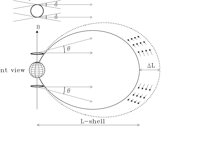
Figure 1: Cartoon showing the geometry of the stellar auroral radio emission. The geometry of the emission beam pattern (ray path deflection angle $\theta$ and opening angle $\delta$) and the auroral ring are displayed. The grey arrows represent the direction of propagation of the rays. The dipole magnetic field lines that identify the auroral cavity are pictured. The small arrows directed toward the star represent the non-thermal electron population that can develop the unstable energy distribution able to drive the ECM emission mechanism.

The hot MCP stars have their magnetospheres dominated by a radiatively-driven stellar wind extending for tens of stellar radii (Trigilio et al., 2004; Leto et al., 2006), whereas many UCDs are very fast rotators, with their magnetospheres dominated by rotation (Schrijver, 2009). The role of the rotational speed to explain the UCD radio activity has been highlighted by many authors (Berger et al., 2008b; McLean et al., 2012). In MCP-type stars, current sheets are formed by the magnetic field lines breaking near the Alfven radius. Similarly in fast-rotating UCDs, there are field-aligned current systems related to the co-rotation breakdown of the magnetospheric plasma, which becomes centrifugally unstable at a distance of tens of stellar radii far from the surface (Nichols et al., 2012). In both cases, electrons can be accelerated up to relativistic energies. Moreover, Nichols et al. (2012) estimate that the power of the electric current systems generated in the fast-rotating magnetospheres is able to sustain the radio luminosity of the UCDs. This non-thermal electron population can develop an unstable energy distribution able to drive the Electron Cyclotron Maser emission observed in some UCDs. These electrons eventually propagate into the deeper magnetospheric regions radiating because of the incoherent gyro-synchrotron mechanism.

The scenario described above is sketched in Fig. 1. The efficiency of the conversion mechanism of the rotationally-induced magnetospheric current systems in radio power decreases with the increasing amount of plasma trapped in the magnetosphere, as a consequence of the reduction of the magnetospheric size due to the larger plasma density (Nichols, 2011; Nichols et al., 2012). The plasma density in the magnetosphere may not be stable over time, if it is provided by a mechanism external to the star, such as a volcanic planet. This may also explain the episodic/seasonal behaviour of the auroral radio emission of the UCDs. This is the case for Jupiter, where the auroral emission is directly affected by the density changes in Io’s plasma torus due to the volcanic activity of this moon (Bonfond et al., 2012; Yoneda et al., 2013). Therefore, by assuming an external volcanic body as the plasma source in the UCD radio-loud magnetospheres, it is possible to explain the unstable auroral radio emission from this kind of objects.

3 The auroral radio emission model

The visibility of the planetary auroral radio emission and the corresponding spectral shape have been successfully modeled for Jupiter (Hess et al., 2008, 2010; Ray & Hess, 2008; Cecconi et al., 2012), and Saturn (Lamy et al., 2008). Following a similar approach, in Paper I we developed a 3D model to study the detectability conditions of the ECM pulses arising from a laminar auroral cavity within a dipolar-shaped stellar magnetosphere. In particular, we proved how the study of the auroral radio-emission features can give hints about the geometry of the overall magnetospheric topology. A section of the auroral radio emission model is sketched in Fig. 1.

Due to the laminar structure of the auroral source region, the emission beam pattern of the amplified radiation will be strongly anisotropic (Louarn & Le Queau, 1996a, b) (see the top view of the ring in Fig. 1). It has been theoretically confirmed that the auroral radio emission is mainly amplified in the direction tangent to the cavity wall (Speir et al., 2014). For a given stellar geometry (rotation axis inclination $i$ and tilt of the dipole axis $\beta$), the model is able to reproduce the auroral radio emission pulse shape and its phase occurrence as a function of the free parameters that control the emission beam pattern. These parameters are the deflection angle $\theta$ and the beaming angle $\delta$. The parameter $\theta$ is the angle between the wave vector $\mathbf{k}$ and the direction perpendicular to the magnetic field vector (roughly shown in the front view of the auroral source region in Fig. 1). The angle $\delta$ quantifies the angular width of the emission beam pattern tangentially directed along the auroral ring.

Table 1: Stellar parameters of TVLM 513-46546.

Fixed Parameters
$R_{\ast}$ - stellar radius [R⊙]	0.103a
$P_{\mathrm{rot}}$ - rotation period [hr]	1.959574b
$i$ - rotation axis inclination [degree]	70
$B_{\mathrm{p}}$ - polar magnetic field [Gauss]	3000c
$\Delta\theta$ - hollow cone width [degree]	4d
Free Parameters	Range	Step
$L$-shell [R∗]	15–40e	5
$\theta$ - deflection angle [degree]	0–25	2.5
$\delta$ - beaming angle [degree]	5–30	5
$\beta$ - magnetic axis obliquity [degree]	0–355	5

• (a) Hallinan et al., 2008; (b) Wolszczan & Route, 2014; (c) Hallinan et al., 2007; (d) Berger et al., 2008a; (e) Nichols et al., 2012.

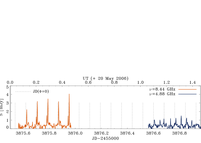
Figure 2: Stokes I measurements of TVLM 513-46546 performed with the VLA at 4.88 (C band) and 8.44 GHz (X band) during two consecutive days. Data already published by Hallinan et al. (2007). Phase bin equal to 0.004. Average time 3 minutes.

Given the frequency $\nu$ and the polar magnetic field strength $B_{\mathrm{p}}$, the grid points where the condition $\nu=s\nu_{\mathrm{B}}$ is verified ($s$ harmonic number) define auroral rings, northern and southern, located above the polar caps, centred on the magnetic dipole axis, and parallel to the magnetic equatorial plane. As a consequence of the magnetic field strength decreasing outwards (for a simple dipole, $B\propto r^{-3}$), the frequency of the auroral radiation originating in rings close to the stellar surface is higher than the radiation emitted in farther rings. The grid points of the magnetospheric cavity where the auroral radio emission can take place are quantified by the $L$-shell parameter of the innermost magnetic field line (that is the distance to the star from the point where the magnetic field line crosses the magnetic equator) and the shell thickness $\Delta L$; these parameters are clearly pictured in Fig. 1.

The model simulation of the auroral radio emission as a function of $\beta$, pointed out that a strict relation between the detectability of the ECM pulses and the ray path deflection ($\theta$) exists. The analysis performed in Paper I showed the existence of two families of auroral light curves: light curves having two doubly-peaked pulses per stellar rotation, with each single peak of opposite polarisation sign; light curves characterised by two single peaks that can be left- or right-hand circularly polarised. The doubly-peaked pulses point to the contributions of the two stellar hemispheres with opposite magnetic field orientation: the auroral radio emission from the northern hemisphere is right-hand circularly polarised (Stokes V ($\mathrm{RCP}-\mathrm{LCP}$) $>0$), while the southern emission is left-hand circularly polarised (Stokes V $<0$).

Given the rotation axis inclination $i$, the phase separation between the peaks with opposite polarisation signs depends on the magnetic axis obliquity ($\beta$) and on the direction of propagation of the wave ($\theta$). The auroral light curves showing only singly-polarised pulses are related to those stellar geometries characterised by a lower tilt of the magnetic dipole axis. In these cases, the effective magnetic field strength does not invert its sign as the star rotates (magnetic curves without zeros) and the auroral beam pattern arising from only one stellar hemisphere will cross the line of sight, if characterised by the appropriate ray path deflection. In general, the deflection angle $\theta$ controls the detectability and the phase location of the auroral pulses, while the beam size of the auroral emission ($\delta$) is directly related to the phase width of the single pulses. The main result obtained in Paper I is that the phase location of the auroral radio pulses provides strong constraints on the geometry of the stellar magnetospheres.

3.1 Simulations of the TVLM 513-46546 auroral radio emission

With the aim to investigate the overall physical conditions of the UCD magnetospheres, we now apply the 3D model of the stellar auroral radio emission to a typical Ultra Cool Dwarf emitting coherent ECM pulses. Among the members of this class of stars emitting auroral radio emission, the M8.5-type dwarf TVLM 513-46546 is the best studied in the radio regime, from 327 MHz (Jaeger et al., 2011) to 95 GHz (Williams et al., 2015b). This source is characterised by quiescent (incoherent) and coherent radio emission. Highly circularly polarised (both left- and right-hand) coherent pulses have been observed in C and X band with the VLA, EVN, and Arecibo radio telescope in many epochs (Berger, 2002; Hallinan et al., 2006, 2007; Berger et al., 2008a; Forbrich & Berger, 2009; Doyle et al., 2010; Yu et al., 2011; Kuznetsov et al., 2012; Route & Wolszczan, 2013; Wolszczan & Route, 2014; Lynch, Mutel & Güdel, 2015; Gawroński, Goździewski & Katarzyński, 2017), but the star was also observed in quiescent status over 6 consecutive rotational periods (Osten et al., 2006). The rotation period of TVLM 513-46546 was derived through diagnostic methods based on infrared photometric monitoring (Lane et al., 2007; Littlefair et al., 2008; Harding et al., 2013). The coherent pulses were phase-folded with the same period. This indicates that the pulsed ECM emission from TVLM 513-46546 is a clear consequence of the stellar rotation (Hallinan et al., 2007), like a light-house effect.

TVLM 513-46546 has a high value of the projected rotational velocity ($v\sin i\approx 60~{}\mathrm{km\,s^{-1}}$; Mohanty & Basri, 2003). Its rotational period ($P_{\mathrm{rot}}$) is about 1.96 hr and is stable over a time scale close to a decade (Wolszczan & Route, 2014). As its radius, we take $R_{\ast}=0.103$ R_⊙, the mean of the values given by Hallinan et al., 2008. The combination of these parameters implies a very large inclination of the rotation axis, $i=70^{\circ}$ (derived from the relation: $v\sin i=2\pi R_{\ast}\sin i/P_{\mathrm{rot}}$). To estimate the stellar magnetospheric size, we take advantage of the analysis performed on this target by Nichols et al. (2012). According to the authors, who adopt a polar field strength $B_{\mathrm{p}}=3000$ Gauss (Hallinan et al., 2007), the magnetic latitude of the last closed field line lies in the range 75^∘–81^∘. From the dipole field line equation, we know $r=L\cos^{2}\lambda$, where $r$ and $\lambda$ are the distance to the centre of the star and the magnetic latitude, respectively. The magnetic latitudes above correspond to a magnetospheric size in the range $\approx 15$–40 stellar radii. The thickness of the auroral cavity ($\Delta L$) has been assumed about 40% of the magnetospheric size, on average. This value has been estimated roughly from the magnetic-latitude range of the transition region where the plasma coronation breakdown occurs ($\lesssim 2.5$ degree, Nichols et al., 2012). As highlighted in Paper I, this parameter has no effect on the simulated auroral radio emission features, hence we fix its value to 40% of the $L$-shell.

In the following simulation step, we fix $B_{\mathrm{p}}=3000$ Gauss. The polar field strength directly affects the spatial location and size of the auroral ring where the ECM emission at a given frequency $\nu$ takes place. As discussed in Paper I, the auroral radio emissions arising from a given magnetospheric cavity, but originating at different heights above the stellar surface, is characterised by almost indistinguishable ECM pulse profiles. This prevents us from giving a priori strong constraints on $B_{\mathrm{p}}$ and/or on the harmonic number $s$, only on the basis of the auroral radio emission detection at a given frequency. The assumed magnetic field strength corresponds to a polar gyro-frequency $\nu_{\mathrm{B}}=8.4$ GHz, whereas at lower magnetic latitudes the auroral source location falls inside the star (for a simple magnetic dipole the equatorial field strength is equal to half of the polar one). To reproduce the auroral radiation at 8.4 GHz outside the stellar surface, we assume that the ECM emission occurs at the second harmonic of the local gyro-frequency, which is equivalent to assuming first-harmonic ECM emission from a dipolar magnetosphere with $B_{\mathrm{p}}=6000$ Gauss.

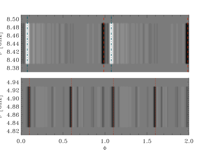
Figure 3: Phase folded light curve of TVLM 513-46546 for the circularly polarised flux (Stokes V). Bottom panel: C band, top panel: X band. Phase bin equal to 0.004.

In the model simulation performed here, we take the angles $\theta$ and $\delta$ that control the auroral radio emission beaming as free parameters. The parameter $\Delta\theta$ is the thickness of the conical sheet where the radiation generated by the elementary ECM-amplification process is beamed. This is related to the velocity of the unstable electron population as follows: $\Delta\theta\approx v/c$ (Melrose & Dulk, 1982). The energy of the emitting electron (about 1 keV) was estimated on the basis of the TVLM 513-46546 X-ray measurements (Berger et al., 2008a). The above electron energy corresponds to an emitting conical sheet $\approx 4^{\circ}$ thick. The last free parameter is the tilt angle $\beta$ of the magnetic dipole axis with respect to the rotation axis.

The model free parameters, the adopted ranges of values, and the corresponding simulation step are summarised in Table 1, for a total of $\approx 2.5\times 10^{4}$ simulated auroral radio light curves. To properly sample the thin auroral cavity close to the stellar surface, the sampling step was taken equal to 0.0225 R_∗.

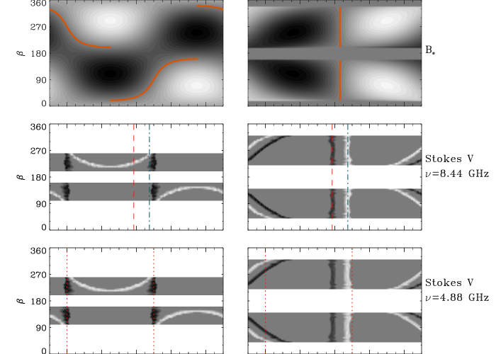
Figure 4: Dynamic synthetic auroral light curves for the C ($\nu=4.88$ GHz, bottom panels) and X band ($\nu=8.44$ GHz, middle panels) obtained as a function of the angle $\beta$. The dotted vertical lines locate the phase occurrence of the 4.88 GHz auroral pulses. The left- and right-handed circularly polarised pulse components at 8.44 GHz are represented with dashed and dot-dashed lines, respectively. The variation of the effective magnetic curve is displayed in the top panels. For the explanation of the 2 cases analysed see the text.

Table 2: Model solutions.

			Case 1: constraints from $\nu=4.88$ GHz				Case 2: constraints from $\nu=8.44$ GHz
$\beta$	$|\beta|$		$\theta$	$\delta$	Pulses		$\theta$	$\delta$	Pulses	$\Delta\Phi$
[degree]	[degree]		[degree]	[degree]			[degree]	[degree]
40	40		-	-	-		10.0	15	RCP+LCP	$-0.001$
45	45		-	-	-		10.0	15	RCP+LCP	0.010
50	50		-	-	-		12.5	15	RCP+LCP	0.020
55	55		-	-	-		12.5	20	RCP+LCP	0.029
60	60		-	-	-		15.0	20	RCP+LCP	0.036
65	65		-	-	-		15.0	20	RCP+LCP	0.043
70	70		-	-	-		15.0	20	RCP+LCP	0.049
75	75		-	-	-		15.0	20	RCP+LCP	0.054
80	80		-	-	-		15.0	20	RCP+LCP	0.060
85	85		-	-	-		15.0	20	RCP+LCP	0.065
90	90		-	-	-		15.0	20	RCP+LCP	0.070
95	85		-	-	-		15.0	20	RCP+LCP	0.075
100	80		5.0	10	RCP+LCP		15.0	20	RCP+LCP	0.080
105	75		5.0	10	RCP+LCP		15.0	20	RCP+LCP	0.086
110	70		7.5	10	RCP+LCP		15.0	20	RCP+LCP	0.091
115	65		7.5	15	RCP+LCP		15.0	20	RCP+LCP	0.097
$120^{{\dagger}}$	60		10.0	15	RCP+LCP		15.0	20	RCP+LCP	0.104
125	55		12.5	20	RCP+LCP		12.5	20	RCP+LCP	0.111
130	50		12.5	20	RCP+LCP		12.5	15	RCP+LCP	0.119
135	45		15.0	20	RCP+LCP		10.0	15	RCP+LCP	0.129
140	40		15.0	20	RCP+LCP		10.0	15	RCP+LCP	0.141
145	35		15.0	20	RCP+LCP		-	-	-	-
150	30		17.5	20	LCP		-	-	-	-
155	25		20.0	20	LCP		-	-	-	-
160	20		20.0	20	LCP		-	-	-	-
200	20		20.0	20	LCP		-	-	-	-
205	25		20.0	20	LCP		-	-	-	-
210	30		17.5	20	LCP		-	-	-	-
215	35		15.0	20	RCP+LCP		-	-	-	-
220	40		15.0	20	RCP+LCP		10.0	15	RCP+LCP	$-0.359$
225	45		15.0	20	RCP+LCP		10.0	15	RCP+LCP	$-0.371$
230	50		12.5	20	RCP+LCP		12.5	15	RCP+LCP	$-0.381$
235	55		12.5	20	RCP+LCP		12.5	20	RCP+LCP	$-0.389$
240	60		10.0	15	RCP+LCP		15.0	20	RCP+LCP	$-0.396$
245	65		7.5	15	RCP+LCP		15.0	20	RCP+LCP	$-0.403$
250	70		7.5	10	RCP+LCP		15.0	20	RCP+LCP	$-0.409$
255	75		5.0	10	RCP+LCP		15.0	20	RCP+LCP	$-0.414$
260	80		5.0	10	RCP+LCP		15.0	20	RCP+LCP	$-0.420$
265	85		-	-	-		15.0	20	RCP+LCP	$-0.425$
270	90		-	-	-		15.0	20	RCP+LCP	$-0.430$
275	85		-	-	-		15.0	20	RCP+LCP	$-0.435$
280	80		-	-	-		15.0	20	RCP+LCP	$-0.440$
285	75		-	-	-		15.0	20	RCP+LCP	$-0.446$
290	70		-	-	-		15.0	20	RCP+LCP	$-0.451$
295	65		-	-	-		15.0	20	RCP+LCP	$-0.457$
300	60		-	-	-		15.0	20	RCP+LCP	$-0.464$
305	55		-	-	-		12.5	20	RCP+LCP	$-0.471$
310	50		-	-	-		12.5	15	RCP+LCP	$-0.480$
315	45		-	-	-		10.0	15	RCP+LCP	$-0.490$
320	40		-	-	-		10.0	15	RCP+LCP	$-0.499$

• ^† Parameters adopted for the simulations of the dynamic spectra performed in Sec. 4, and for the simulations of the X band ($\nu=8.44$ GHz) light curves performed in Sec. 6

3.2 VLA observations of TVLM 513-46546

To identify the set of free parameters able to reproduce the TVLM 513-46546 auroral radio emission, the model simulations must be compared with real multi-wavelength observations of this target. As previously highlighted, the radio emission features of the UCDs are not stable within all the observing epochs. With the aim to minimise the source variability, we selected a data set where the source TVLM 513-46546 was characterised by an almost stable auroral radio emission lasting for several stellar rotation periods. The observing epoch here analysed refers to the VLA measurements of TVLM 513-46546 performed on May 2006 at 8.44 ($\approx 9.75$ hours on May 20th) and 4.88 GHz ($\approx 9.75$ hours on May 21st), within a bandwidth 100 MHz wide, already published by Hallinan et al. (2007). These data have been re-analysed using the standard procedures of the Astronomical Image Processing System (AIPS). The observed light curves for the Stokes I in C (4.88 GHz) and X (8.44 GHz) bands are shown in Fig. 2.

We analyse the present observing epoch because TVLM 513-46546 has passed through a stable active phase, showing ECM pulses at every rotation period. This could help us to simulate the true modulation effect of its auroral radio emission without suffering from the intrinsic source variability. The measurements performed on May 20th at 8.44 GHz lasted about 5 consecutive rotation periods and periodic doubly-peaked pulses are clearly detected. Periodic pulses have been clearly detected also at 4.88 GHz, during the other 5 consecutive rotation periods observed on May 21st, but with a lower peak level (see Fig. 2).

These VLA measurements were phase folded using the ephemeris given by Wolszczan & Route (2014):

$\mathrm{MJD}=2\,456\,188.65+0.0816489E~{}~{}\mathrm{[days]}$.

The phase-folded light curves for the circularly polarised flux density (Stokes V), are shown in Fig. 3 for both C and X bands. As discussed by Hallinan et al. (2007), the doubly-peaked pulses detected in X band have opposite polarisation signs (see Fig. 3 top panel), and lie in the range of phases $\approx 0.95$–1.1. The light curve for the C band is instead characterised by two pulses per spin period that are left-hand circularly polarised ($\Phi\approx 0.1$ and $\Phi\approx 0.6$, Fig. 3 bottom panel). Both pulses have a similar phase duration of about 5% of the rotational period.

3.3 Comparison between simulations and observations

In the next step, we compare the model simulations with the observations, assuming that the source is stable within the analysed epoch. The differences between the two observing bands are assumed as an intrinsic frequency-dependent effect.

The analysis of the auroral radio emission from TVLM 513-46546 aims at achieving a deep knowledge of its magnetosphere. First of all, we noticed that the size of the auroral cavity has null effect on the simulated pulses, confirming the results obtained in Paper I. Above $\approx 10$ R_∗ the $L$-shell parameter does not affect the phase location and the shape of the ECM pulses. The features of the auroral radio emission from TVLM 513-46546 (described in Sec. 3.2) indicate that the magnetic curve extremes should be located at intermediate phases between the two pulses observed in C band. On the other hand, the doubly-peaked structure (with single peaks of opposite polarisation) detected in the X band gives a clear indication that it is sampling the rotational transition from the southern to the northern stellar hemisphere. In fact, each stellar hemisphere contributes to the auroral radio emission with radiation of opposite polarisation. The null of the magnetic curve will then be falling at an intermediate phase between the pulses of opposite signs detected in X band.

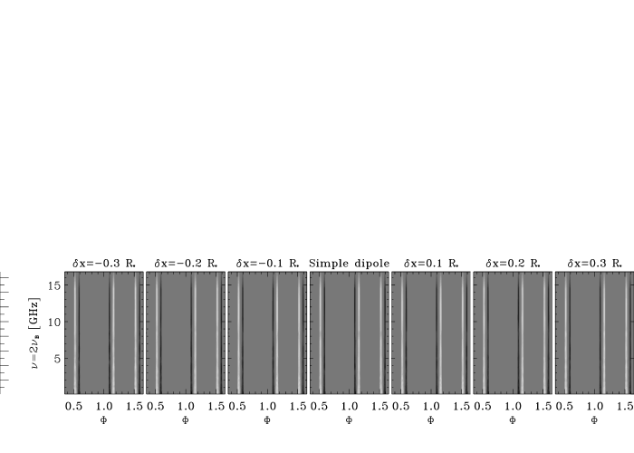
Figure 5: Simulated dynamic spectra of the auroral radio emission of TVLM 513-46546 as a function of the dipole shift. Dipole shifted along the $x$-axis: top panels. Dipole shifted along the $y$-axis: middle panels. Dipole shifted along the $z$-axis: bottom panels. The further axes displayed on the left side of the figures indicates the auroral radio emission frequency in case of ECM at the first harmonic of the local gyro-frequency. The corresponding distances of the radiating layers are listed in the right panels axes.

Following these two robust observational constraints, we separately analyse the case of a magnetic stellar geometry with a $B$ maximum at $\Phi\approx 0.85$ (Case 1) and the case where the stellar geometry is characterised by a $B$ null at $\Phi\approx 0.025$ (Case 2). The simulated light curves of the auroral radio emission (for the C and X bands), that verify the imposed conditions, are shown in Fig. 4. The left panels of Fig. 4 show the magnetic curves (top panel) and the modelled auroral light curves, for the X (middle panel) and C (bottom panel) bands. These curves simulate the auroral pulses from a magnetosphere with an effective magnetic field curve characterised by extremes falling at intermediate phases between the C band peaks. The right panels of Fig. 4 show the simulation from a magnetosphere characterised by an effective magnetic curve with a null between the doubly-peaked pulses detected in X band. The magnetic curves that do not invert the sign of the effective magnetic field strength (absence of nulls) are not shown. This explains the grey bands of the top right panel of Fig. 4.

In Table 2, we summarise the model solutions achieved separately for the two cases. For Case 2, the parameter $\Delta\Phi$ is also reported. This parameter is the phase shift between the phase location of the magnetic null (negative to positive magnetic field strength) for the two cases analysed. The parameter can be visually estimated by looking at the solid lines in the top panels of Fig. 4. It also quantifies the different spatial orientation of the magnetospheres that satisfies the imposed conditions related to the two geometrical cases under analysis. The magnitude of the phase shift is necessary to locate exactly the phase position of the 8.44 GHz doubly-peaked auroral pulse and is a function of the dipole tilt $\beta$. We found that the values of this parameter that are able to simulate the observed auroral features in both the C and the X bands lie in the ranges $100^{\circ}$–$140^{\circ}$ and $220^{\circ}$–$260^{\circ}$, corresponding to an absolute value of the tilt $\beta$ between the dipole and the rotation axis in the range $40^{\circ}<|\beta|<80^{\circ}$. A less tilted dipolar magnetosphere is not able to reproduce the auroral pattern observed at 8.44 GHz, whereas a larger misalignment of the oblique rotator cannot reproduce the timing of the pulses detected at 4.88 GHz.

Those simulations performed assuming a simple dipole indicate that a phase lag must be introduced between the light curves at the two simulated frequencies, as evidenced by $\Delta\Phi\neq 0$. This suggests that the orientations of the magnetospheres able to reproduce the C and the X bands are not the same. It seems that there is not a common dipolar geometry able to reproduce simultaneously the phase locations of the auroral pulses detected at 4.88 and 8.44 GHz.

4 Auroral radio emission from a non-dipolar magnetosphere

The model used to simulate the auroral radio emission of TVLM 513-46546 was developed under the simplified hypothesis of magnetic field dipolar topology. But the true magnetic field topology of this fully convective ultra cool dwarf could be far from a simple dipole. Recently the magnetic field generation in the low mass rapidly rotating fully convective stars has been simulated using three-dimensional magnetohydrodynamic models (Yadav et al., 2015). These simulations were able to reproduce the kGauss level of the magnetic field strength measured in some UCDs (Reiners & Basri, 2007, 2010), and the dipole-dominated magnetic field topology often observed in the mid M dwarfs (Donati et al., 2006; Morin et al., 2008a, b), but was also able to simultaneously simulate the presence of a small scale (toroidal) magnetic component, that characterises some late M type dwarfs (Morin et al., 2010).

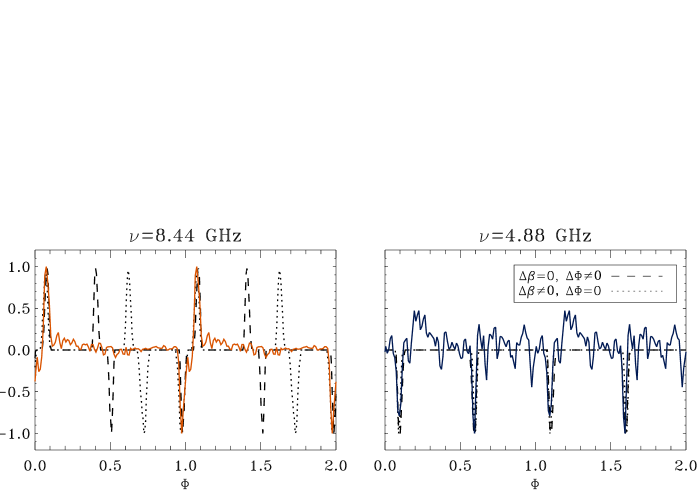
Figure 6: Comparison between the observed and the simulated auroral radio light curves of TVLM 513-46546. Auroral emission at 8.44 GHz (X band): left panel. Auroral emission at 4.88 GHz (C band): right panel. The dashed line refers to the simulations performed assuming a common magnetospheric geometry for the X and C band emission; to reproduce the observed timing of the auroral pulses, we introduced a phase-lag between the light curves simulated at the two frequencies. The dotted line refers to simulations arising from magnetospheres with different dipole tilt; in this case, there is no phase lag between the light curves simulated at the X and C bands. The C band synthetic curves were simulated assuming a dipole shifted along the dipole axis ($z$-axis) toward the south pole ($\delta z=-0.3$ R_∗). The X band simulations were performed assuming a simple dipole, which is equivalent to assume a dipole shifted along the $x$ or $y$-axes.

To take into account the non-dipolar topology of the UCD magnetic field, we modified the model described in Paper I to reproduce the auroral radio emission from a stellar magnetosphere shaped like an offset dipole. This could be assumed as a first approximation of a non-dipolar magnetic field topology, and was commonly used to reproduce the complex magnetic field curves measured in some hot magnetic stars (Hatzes, 1997; Glagolevskij, 2011; Oksala et al., 2012, 2015).

In the following, we analyse the frequency dependence of the stellar auroral radio emission visibility as a function of the dipole shift, along and across the axis passing through the centre of the star and parallel to the dipole magnetic axis. The stellar reference frame ($Oxyz$) is anchored with the stellar centre, has the $z$-axis parallel or coincident with the dipole axis, and the $x$-axis is located in the plane passing through the $z$-axis and containing the rotation axis. Details of the method used are given in Appendix A.

In Fig. 5, we show the simulated dynamical spectrum of the auroral radio emission from the magnetosphere of TVLM 513-46546 shaped like an offset dipole, and constrained to have the maximum magnetic field strength at the stellar surface not exceeding 3000 Gauss. The frequency range analysed is 16.88–0.1 GHz (8.44–0.05 GHz if the auroral emission is generated at the first harmonic of the local gyro-frequency). The higher frequency limit has been chosen on the basis of the value of the first harmonic of the gyro-frequency at the stellar surface ($B_{\mathrm{p}}=3000$ Gauss), whereas the low-frequency limit is close to the lower limit of the frequency range of the new-generation Earth-based low-frequency radio interferometers, such as the Low-Frequency Array (LOFAR; van Haarlem et al., 2013), the Murchison Widefield Array (MWA; Tingay et al., 2013), or the forthcoming Square Kilometre Array (SKA). The selected frequency range corresponds to the heights above the stellar surface that lie in the range $\approx 0$–4.5 [R_∗]. The simulations have been performed assuming for each analysed frequency the same emission beam pattern (in particular $\delta=15^{\circ}$ and $\theta=10^{\circ}$) and a common tilt of the magnetic axis ($|\beta|=60^{\circ}$). The simulations have been performed varying the dipole shift along the $xyz$-axes in the range from $-0.3$ to 0.3 [R_∗], with a step of 0.1 [R_∗].

The results of the dynamical spectra simulations from an offset-dipole are shown in Fig. 5. By looking at the figure, it is clear that the dipole offset along the $x$-axis or the $y$-axis has negligible effect on the simulated dynamic spectra and consequently on the auroral light-curve shape. In these cases, the corresponding simulated dynamic spectra are almost indistinguishable from the case of auroral emission from a simply dipolarly-shaped magnetosphere. When the dipole is shifted along the $z$-axis, coinciding with the dipole axis, this determines a north-south asymmetry that significantly affects the stellar auroral radio-emission visibility (see bottom panels of Fig. 5). The spectral dependence of the auroral radio emission arising from each stellar hemisphere becomes progressively asymmetric as the dipole shift increases. The auroral radio emission arising from the hemisphere where the dipole approaches the stellar surface is almost unchanged, whereas the emission from the opposite hemisphere progressively disappears, as the radio frequency increases. This effect depends on the amplitude of the dipole shift from the centre of the star.

To deeply explore the effect of the offset dipole on the auroral radio emission visibility from TVLM 513-46546, we performed simulations, tuned at the C and X observing bands, using the parameters listed in Table 2. The dipole location was shifted along the $xyz$-axes. These new sets of simulations are pictured in Figs. 13 and 14.

As examples of the simulated auroral radio light curves, we show in Fig. 6 the observed auroral emission with two representative simulated curves superimposed; the left panel refers to the pulses detected at 8.44 GHz, the right panel to that at 4.88 GHz. The two sets of model parameters used to simulate the auroral light curves shown in Fig. 6 were selected to reproduce two possible cases. In the first case, we simulated light curves at 4.88 and 8.44 GHz without phase lag, but the two corresponding stellar geometries are not the same ($\Delta\Phi=0$ and $\Delta\beta\neq 0$): the adopted dipole tilts are $\beta=40^{\circ}$ at 8.44 GHz and $\beta=100^{\circ}$ at 4.88 GHz ($\Delta\beta$ minimun). In the second case, we simulated the auroral emission at the two observing frequencies using the same stellar geometry (in particular we assumed $\beta=120^{\circ}$), but we needed to introduce a phase lag between the two light curves at the two frequencies ($\Delta\beta=0$ and $\Delta\Phi\neq 0$). The corresponding combination of the parameters that control the auroral beam pattern are listed in Table 2.

The 4.88 GHz synthetic curves in Fig. 6 were obtained using a dipole shifted along the dipole axis (in particular $\delta z=-0.3$ R_∗). The curves at 8.44 GHz was instead obtained assuming a simple dipole, which is equivalent to the cases of an offset-dipole along the $x$ or $y$-axes. The effect of the dipole shift along the $z$-axis makes it easier to reproduce the auroral peaks detected at the lower frequency (4.88 GHz). In fact, the auroral component arising from the northern hemisphere, expected RCP circularly polarised, is naturally suppressed by the displacement of the dipole in the direction to the south pole. The auroral features detected at the higher frequencies (8.44 GHz) are instead not compatible with an offset dipole along the polar axis. In fact, a general result of our simulations is that if the northern signature of the auroral emission at 4.88 GHz disappears, then there cannot be auroral radio emission radiated at frequencies higher than 4.88 GHz.

In the case of the auroral radio emission from an offset dipole, we have not found a common magnetospheric geometry that is able to simultaneously reproduce the timing and pattern of the auroral pulses detected at the two observing radio frequencies (4.88 and 8.44 GHz). We reach the same conclusion obtained for the case of the auroral radio emission arising from a simple dipolar magnetosphere (Sec. 3). The geometry of the TVLM 513-46546 magnetosphere able to reproduce the auroral pulses detected at 8.44 GHz is not the same as that adopted to simulate the 4.88 GHz pulses.

5 The magnetosphere of TVLM 513-46546

Like the case of Jupiter, where the study of the planet auroral radio emission was able to constrain the topology of its magnetosphere (Hess et al., 2010, 2011), the analysis of the stellar auroral radio emission arising from the UCD TVLM 513-46546 can be used to obtain indirect information regarding the overall field topology of the stellar magnetosphere. The auroral radio emission gives a snapshot of the stellar magnetic field topology at the epoch of its detection, and its modelling has been already used as a method to describe the field topology of UCD magnetospheres (Metodieva et al., 2017).

To use this coherent phenomenon as a tool to investigate the stellar magnetospheric configuration, it is necessary to assume the temporal stability of the stellar magnetic-field topology over the time range spanned by the measurements. In the case of TVLM 513-46546, even though the two bands are not observed simultaneously, this is a fully sensible hypothesis, also supported by the almost simultaneous C and X broad-band observations performed with the Karl G. Jansky Very Large Array (JVLA) during other active epochs of TVLM 513-46546, which display a very similar behaviour (Lynch et al., 2015). This similarity supports the hypothesis of the temporal stability of the overall magnetic-field topology of the TVLM 513-46546 magnetosphere, over a time of $\approx 10$ years.

5.1 Torqued magnetosphere

The modelling of the phase occurrence of the TVLM 513-46546 pulses (Sections 3 and 4) highlights that the beams of the auroral emission at 8.44 (X band) and 4.88 GHz (C band) have to be misaligned. As discussed in Paper I, the elementary physical process responsible for the stellar auroral radio emission is the Electron Cyclotron Maser (ECM). The orientation of the highly-beamed ECM emission pattern is strongly related to the orientation of the magnetic-field vector in the region where it takes place. The phase lag of the 4.88 GHz pulses could then be explained as a consequence of a different orientation of the magnetic-field vector with respect to the auroral region where the 8.44 GHz emission takes place. This is displayed in Fig. 7, where the orientations of the auroral beams at the two radio frequencies here analysed are shown. The figure is related to the minimum value of $\Delta\Phi$ listed in Table 2 ($\Delta\Phi=0.08$ with $\beta=100^{\circ}$). It is a consequence that the magnetic field lines passing trough the cavity boundaries where the two frequencies arise have to be bent. The dynamics of the plasma of the fast rotating UCD TVLM 513-46546 could give rise to a torqued magnetosphere, like in Jupiter (Hill et al., 1974; Hill, 1979). In principle, the auroral radio emission arising from a torqued magnetosphere could explain the timing of the radio pulses from TVLM 513-46546, but this scenario is affected by a paradox.

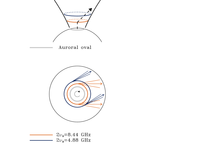
Figure 7: Top panel, side view of the auroral cavity that radiates at 4.88 and 8.44 GHz (assuming $B_{\mathrm{p}}=3000$ [Gauss]). The footprint at the stellar surface is also pictured (auroral oval). In the bottom panel is shown the top view of the auroral cavity. The auroral beam pattern at the two analysed frequencies are shown. The corresponding bended magnetic field line is schematically pictured in the top panel (dashed line).

In the case of a simple dipolar magnetic topology (Sec. 3), our simulations evidence that there is no stellar geometry able to produce LCP C band auroral radio emission and simultaneously LCP+RCP X band pulses. To reproduce auroral radio emission arising at a given radio frequency from only one hemisphere, one needs to assume an offset dipole along the polar axis ($z$-axis), see Sec. 4. Due to the direct stellar magnetic-field strength dependence, the X band (8.44 GHz) pulses originate from a magnetospheric region closer to the stellar surface, when compared with the location of the ring in which the C band (4.88 GHz) pulses arise. In the top panel of Fig. 7, we show the side view of the auroral rings above the magnetic pole where the pulsed emission of TVLM 513-46546 originated. The simulations with an offset dipole show that the auroral component arising from the hemisphere from which the dipole is moving away suffers from a high-frequency cutoff, as the dipole is shifted along the polar axis (see bottom panels of Fig. 5). The auroral emission at the radio frequencies generated close to the star are affected earlier by the offset dipole.

The paradox is that while the auroral emission at 8.44 GHz arising from the northern hemisphere should be suppressed, the RCP component (Stokes $\mathrm{V}>0$) of the X band auroral pulse is instead clearly detected (left panel of Fig. 6).

5.2 Two distinct auroral cavities

As previously discussed (Sec. 4), the magnetic-field topology of fast-rotating fully-convective low-mass stars could be characterised by the coexistence of large- and small-scale magnetic fields (Yadav et al., 2015). The large-scale field component is well described by a magnetic field with an overall axial symmetry (dipole or offset dipole), whereas the small-scale magnetic-field components have a toroidal topology. For the fast-rotating UCD TVLM 513-46546, it is therefore reasonable to assume a similar magnetic-field configuration.

The difference between the C and X band TVLM 513-46546 auroral emission could be explained if the coherent pulses at 4.88 and 8.44 GHz originate from two different auroral cavities, related to two distinct magnetic-field components. The cavity where the LCP pulses at 4.88 GHz originate would be related to a large magnetic cavity with footprints close to the poles, shaped like a dipole shifted along the polar axis. The LCP+RCP 8.44 GHz auroral pulses would instead arise from a more internal cavity, related to small-scale magnetic structures (like magnetic loops with equator-ward footprints). If the regions with opposite magnetic-field polarity of this small-scale auroral cavity both have magnetic-field strength large enough to radiate auroral radio emission at 8.44 GHz, then auroral pulse components of opposite polarisations will be detectable. The meridian plane containing the magnetic-field lines delimiting the small-scale auroral cavity may not be closely related with the geometry of the large-scale magnetic-field topology. The large- and small-scale auroral cavities could then be described by two distinct magnetic-dipole orientations. The possible existence of two distinct auroral cavities could therefore explain the phase lag of the 4.88 GHz pulses with respect to those detected at 8.44 GHz.

The non-detection in the C band of the auroral features observed in the X band (LCP+RCP auroral pulse), and viceversa, can be used to constrain the magnetic-field strength of the footprints of the auroral cavities. In the case of the loss-cone driven ECM emission mechanism, the deflection angle $\theta$ is directly related to the hollow cone half-aperture $\theta_{\mathrm{B}}$, where the radiation amplified by the elementary emission process is beamed (in the case of the northern hemisphere auroral emission $\theta=90^{\circ}-\theta_{\mathrm{B}}$). Furthermore, the hollow cone half-aperture is a function of the frequency of the amplified radiation as follows: $\cos\theta_{\mathrm{B}}=v/c\sqrt{1-\nu_{\mathrm{B}}/\nu_{\mathrm{B_{max}}}}$ (Hess et al., 2008), with $v$ the speed of the unstable electrons and $\nu_{\mathrm{B_{max}}}$ gyro-frequency at the stellar surface. The model free parameters ($\theta$ and $\delta$) that reproduce the auroral radio emission detected at 8.44 GHz are reported in Table 2. In the cases of the solutions for the X band, if the emission beam pattern is deflected of further 2.5–5 degrees it does not intercept the line of sight and the auroral radio emission will not be detectable. Assuming that the 4.88 GHz emission suffers from the above determined further deflection, it is then possible to estimate the gyro-frequency at the stellar surface and then the magnetic field strength by using the relation between $\theta_{\mathrm{B}}$ and $\nu_{\mathrm{B_{max}}}$ written above, given the deflection angles at two different values of the gyro-frequency. The corresponding values of the magnetic-field strength at the stellar surface lie in the range $\approx 2000$–3300 Gauss. The estimation above gives only a rough constraint to the magnetic-field strength. To obtain a more refined magnetic-field strength estimation at the footprints of the equator-ward toroidal magnetic-field lines, it is necessary to measure the high-frequency cutoff of the auroral pulses of opposite polarisation. This measurement can be obtained only by acquiring the wide-band dynamical spectrum of the stellar auroral radio emission.

At the opposite of the 8.44 GHz emission, the 4.88 GHz coherent pulses take place in the large auroral cavity ($L=15$–40 R_∗ corresponding to $75^{\circ}<\lambda<81^{\circ}$) and do not have a counterpart at 8.44 GHz (Fig. 3 and Fig. 6). This high frequency cutoff can be easily explained if the magnetic field strength at the south pole is $<1500$ Gauss. In this case, the second harmonic at the stellar surface is $<8.44$ GHz and the corresponding ECM emission will be not amplified. If the amplified emission frequency is the first harmonic of the local gyro-frequency, then the estimated values of the magnetic field strengths double.

Figure 8: Density of the refractive plasma as a function of the incident angle able to deflect the X band ($\nu=8.44$ GHz) auroral emission, amplified by a pure horseshoe driven ECM mechanism, of the values that fit the observations.

The discussion made so far has been done under the assumption of vacuum propagation. The possible existence of layers of thermal plasma around the star implies the deflection of the ray path. This additional contribution to the ray path deflection needs a lower hollow-cone half aperture (for the loss-cone driven ECM emission mechanism) to make the auroral radio emission of the innermost cavity undetectable at the lower frequency ($\nu\leq 8.44$ GHz), thus causing the enhancement of the magnetic-field strength at the stellar surface.

The refractive effects are quantified by the Snell law: $\sin\alpha_{\mathrm{r}}=\sin\alpha_{\mathrm{i}}/n_{\mathrm{refr}}$, where $\alpha_{\mathrm{i}}$ and $\alpha_{\mathrm{r}}$ are the angles of incidence and refraction and $n_{\mathrm{refr}}$ the refractive index of the medium. In the case of the extraordinary magneto-ionic mode and for a propagation parallel to the local magnetic field, the refractive index can be written as $n_{\mathrm{refr}}^{2}=1-\nu_{\mathrm{p}}^{2}/(\nu^{2}-\nu\nu_{\mathrm{B}})$ ($\nu_{\mathrm{p}}\approx 9\times 10^{-6}\sqrt{N_{\mathrm{e}}}$ GHz plasma frequency of the thermal electrons with number density $N_{\mathrm{e}}$). If the auroral radio emission is amplified by a pure horseshoe-driven ECM elementary emitting process, the ray path is perpendicular to the local magnetic field at all frequencies. Under this assumption, it is possible to evaluate the electron number density necessary to deflect the horseshoe-driven auroral emission exactly of the angle $\theta$, reported in Table 2. In Fig. 8 we show the electron number density of the refractive layer, that deflects the auroral ray path generated at 8.44 GHz, as a function of the incident angle. The values of electron density thus estimated are incompatible with the wave propagation at 4.88 GHz. In fact, the lower frequency waves cannot freely propagate at the corresponding refraction indices. This allows us to exclude the horseshoe-driven ECM as the leading emission mechanism, confirming the conclusion of Lynch et al. (2015) that the auroral radio emission of TVLM 513-4654 is driven by the loss-cone instability. However, the presence of a lower density refractive plasma ($N_{\mathrm{e}}<10^{10}$ cm^-3) that concurs to the ray path defection of the auroral plasma cannot be ruled out. Furthermore, the spatial orientation of such refraction planes can introduce a frequency-dependent longitudinal deflection of the auroral radiation. This effect can take into account the measured phase shift between the light curves at 4.88 and 8.44 GHz.

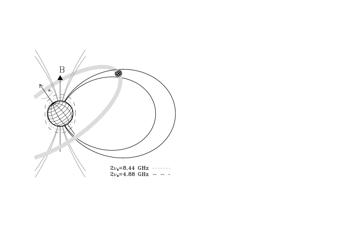
Figure 9: Planet orbit within the magnetosphere of TVLM 513-46546; angles and size are not in scale. The magnetic field lines that are crossed by the planet are displayed using the thick black lines. The magnetic field lines of the cavity with footprints at high magnetic latitudes are shown by the light grey magnetic field lines. The cross section of the equipotential surface of a simple dipole with $B_{\mathrm{P}}=3000$ Gauss is also displayed. The magnetic strengths analysed correspond to the second harmonic of the local gyro-frequency that are equal to 4.88 and 8.44 GHz.

6 Planet-induced auroral emission

To explain the observed differences between the auroral pulses detected at 4.88 and 8.44 GHz (the phase lag and the circularly polarised features), we have examined two possible scenarios in the previous section. In particular, we propose the existence of two distinct auroral cavities, where the emission at the two observing frequencies originates.

The analysis performed in the Sec. 3 and Sec. 4 highlights how the auroral radio emission arising from the whole stellar magnetosphere generates two pulses per stellar rotation, each pulse being singly or doubly peaked with opposite polarisation sense. On the contrary, the auroral features of TVLM 513-46546 detected at 8.44 GHz are characterised by only one doubly-peaked pulse per stellar rotation. Such observational evidence could be explained if the auroral cavity, where the 8.44 GHz emission originates, is constrained within a small range of magnetic longitudes.

To explain some features of the auroral radio emission of UCDs, some authors have proposed a scenario like the Io-Jupiter interaction, where the Io-DAM emission originates in the Io’s flux tube. Recently, Hallinan et al. (2015) suggested the existence of magnetic interaction between the stellar magnetosphere and one orbiting exoplanet to explain the auroral radio emission modulation of the UCD LSR J1835+3259. This supports the idea that, at the bottom of the main sequence, the stellar auroral radio emission can be also powered by the magnetic interactions with rocky planets orbiting around ultra cool and brown dwarfs. The indication of the existence of big dust grains (millimetre size) in debris disks around brown dwarfs (Ricci et al., 2012, 2013) makes it possible to form rocky planets around very low-mass UCD stars. Direct confirmation of the existence of rocky planets around the UCDs is given by the recent discovery of Earth like planets orbiting around the M8 type dwarf 2MASS J23062928-0502285 (TRAPPIST-1) (Gillon et al., 2017).

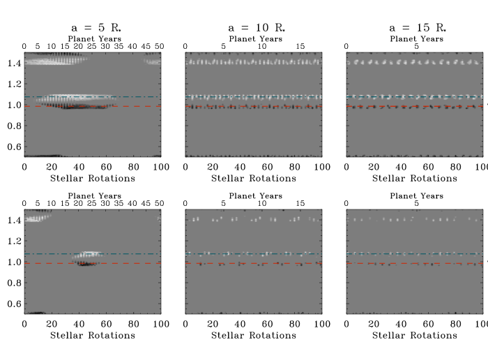
Figure 10: Simulated evolution of the auroral radio light curve of TVLM 513-46546. The planet orbital plane was assumed coinciding with the stellar rotation plane. The light curves are calculated over a time range that spans 100 stellar rotations. The displayed dynamic light curves simulate the auroral radio emission arising from a magnetic flux tube triggered by an orbiting planet. The simulated light curve changes as a function of the planet position inside the stellar magnetosphere. Different sizes of the exoplanet orbital radius have been analysed, the corresponding values of planetary revolution periods are reported in the top x-axis of the figures. The simulations have been performed assuming two different values of the thickness of the flux tube, $\Delta=90^{\circ}$ (top panels) and $\Delta=30^{\circ}$ (bottom panels). The dashed and the dot-dashed horizontal lines represent, respectively, the left- and right-handed circularly polarised pulse components detected at 8.44 GHz.

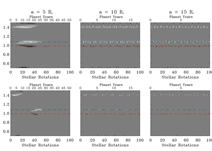
Figure 11: Caption similar to the case of Fig. 10. The simulations pictured in figure were obtained assuming an orbiting plane inclined of $30^{\circ}$ respect to the star rotation plane.

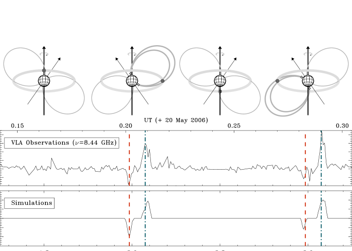
Figure 12: Top panels: cartoon showing the magnetospheric orientation of TVLM 513-46546 and the corresponding planet orbital position able to trigger the stellar auroral radio emission beamed along directions observable from the Earth. Middle panel: light curve of TVLM 513-46546 observed at 8.44 GHz lasting 2 consecutive stellar rotations. Bottom panel: two consecutive simulated auroral light curves captured from an active season of the star. The simulations of these light curves have been carried out assuming the closer orbital configuration and the slimmer flux tube size; simulations shown on the bottom left panel of Fig. 10. The dashed and the dot-dashed vertical lines individuate, respectively, the left- and the right-handed circularly polarised pulse components detected at 8.44 GHz. The cartoon and the simulations refer to the case of planet orbital plane coinciding with the stellar rotation plane.

We analyse if the auroral radio emission induced by the star-planet interaction could be applied to the case of TVLM 513-46546. Hess & Zarka (2011) have extensively analysed the auroral radio emission induced by the star planet interaction as a tool to derive information regarding the geometry of the system. The authors take into account two possible origins of the auroral radio emission: the case of auroral radio emission from the star induced by the exoplanet (analogous to the case of auroral radio emission in Jupiter, controlled by the moon Io) and the case of emission from the magnetosphere of the exoplanet induced by the stellar wind. The high-frequency cutoff of the auroral radio emission is directly related to the magnetic-field strength at the surface of the object where it takes place, be it the star or the planet. The magnetic-field strength of exoplanets is expected to be comparable to the magnitude of the magnetic-field strength of Jupiter (few Gauss). The auroral radio emission from the exoplanet, powered by the wind of the parent star (Nichols & Milan, 2016), can be explored in the low-frequency radio domain. Because of the strength of the magnetic-field deduced from the analysis of the auroral radio emission in TVLM 513-46546 (at the kGauss level), the case of the auroral radio emission arising from the stellar flux tube crossing the exoplanet seems more plausible. This scenario is shown in Fig. 9, where it is possible to distinguish two auroral cavities. The poleward cavity where the 4.88 GHz originates is related to the centrifugally-opened field lines. Far from the star, these lines locate the system of currents generated by the centrifugal force (Nichols et al., 2012). The equatorward cavity, responsible of the 8.44 GHz auroral emission, is instead related to the flux tube excited by the planet. The combined auroral emissions arising from the flux tubes crossing the planet and from the auroral cavity involving the whole magnetosphere could be responsible for the different auroral features observed at 4.88 and 8.44 GHz in TVLM 513-46546.

The stellar auroral radio emission triggered by an external body is modulated by the orbital period of the planet (Hess & Zarka, 2011). To check if the planet-induced auroral radio emission could be a plausible scenario for TVLM 513-46546, we performed simulations of the auroral radio emission arising only from the flux tube excited by a small body orbiting close to the star, not from the full auroral ring. The frequency of the simulated auroral radio emission is equal to 8.44 GHz, and the field topology of the small scale stellar magnetic loops was approximated by a simple dipole. The upper limit to the orbital radius ($a$) of the planet is assumed less or equal to the minimum magnetospheric size adopted in the previous simulations (15 R_∗). This is to take into account the results obtained by Kuznetsov et al. (2012) who conclude that an external body $\approx 24$ stellar radii away from TVLM 513-46546 would not be able to explain the timing of its auroral radio emission. The analysed values of the planet orbital radius $a$ are: 5, 10, and 15 stellar radii. Two possible inclinations of the orbital plane have been taken into account: the case of a planet orbiting in the plane defined by the stellar rotation and the case of a planet with orbital plane inclined of $30^{\circ}$.

The stellar mass of TVLM 513-46546 is about 0.07 M_⊙ (Dahn et al., 2002). Applying the third Kepler’s law, the chosen values of the orbital radii give planet orbital periods of 1.98, 5.61, and 10.31 times the stellar rotation period, respectively ($P_{\mathrm{rot}}\approx 1.96$ hours). For the magnetic sector of the active flux tube, two cases have been analysed. In the first one, the angle at the centre ($\Delta$) of the magnetic sector is fixed equal to $90^{\circ}$, similar to the longitudinal extension of the tail following the spot of Io’s induced aurora, as observed in the ultraviolet images of Jupiter (Clarke et al., 2002). In the other case, the angle $\Delta$ is assumed equal to $30^{\circ}$. We adopt $\beta=120^{\circ}$ (central value of the estimated range given in Table 2, equivalent to a dipole absolute tilt of $60^{\circ}$). The corresponding parameters that control the auroral beam pattern ($\delta$ and $\theta$) are reported in Table 2. We discard the hypothesis $\beta=360^{\circ}-120^{\circ}=240^{\circ}$, because this assumption implies a too large $\Delta\Phi$ value.

For the cases analysed here, we simulated the light curves as a function of the planet orbital position. Such simulated dynamic auroral light curves are shown in Figs. 10 and 11. In the case of auroral emission induced in the thicker flux tube ($\Delta=90^{\circ}$), we find a high occurrence of the phenomenon; see the top panels of Fig. 10 and Fig. 11. In particular, in the case of the planet orbital plane coinciding with the stellar rotation plane, during 100 consecutive stellar rotations the pulses are detectable in many stellar periods. The percentage of periods characterised by at least one pulse are: 82% assuming planet orbital radius $a=5$ R_∗ (82% RCP, 74% LCP); 91% with $a=10$ R_∗ (91% RCP, 89% LCP); 80% with $a=15$ R_∗ (78% RCP, 77% LCP). The auroral pulse detection rate, estimated for the case of the orbital plane inclined of $30^{\circ}$, are instead: 78% with $a=5$ R_∗ (68% RCP, 60% LCP); 91% with $a=10$ R_∗ (91% RCP, 69% LCP); 80% with $a=15$ R_∗ (78% RCP, 62% LCP). In the case of auroral radio emission arising from a planet flux tube followed by a long tail, the simulations generally predict light curves characterised by the occurrence of two pulses (doubly or singly peaked) per stellar rotation. An exception to this are the simulations in which the planet is closer to the star (5 R_∗), predicting periods during which we observe two pulses per stellar rotation, periods with one pulse per rotation, and quiet periods. Such seasonal periodicity of the pulse occurrence is clearly highlighted only in this case. The analysis of the occurrence of the auroral emission simulated in the case of the slimmer flux tube ($\Delta=30^{\circ}$), bottom panels of Fig. 10 and Fig. 11, shows a lower detection rate. In the case of orbital plane coinciding with the stellar rotation plane the detection rates are: 43% with $a=5$ R_∗ (41% RCP, 35% LCP); 49% with $a=10$ R_∗ (36% RCP, 32% LCP); 42% with $a=15$ R_∗ (31% RCP, 27% LCP). Whereas in the case of orbital plane inclined of $30^{\circ}$, the detection rates are: 41% with $a=5$ R_∗ (41% RCP, 18% LCP); 47% with $a=10$ R_∗ (37% RCP, 16% LCP); 36% with $a=15$ R_∗ (25% RCP, 16% LCP). This happens because in the case of the thick flux tube ($\Delta=90^{\circ}$) it is possible to have a number of planet orbital positions able to cause a detectable auroral radio emission larger than that obtainable in the case of a thin flux tube ($\Delta=30^{\circ}$). We also note that, for the adopted stellar geometry, the detection of right-hand circularly polarised (RCP) pulses is favoured for every combination of the model parameters chosen to characterise the planet-induced auroral emission. These conclusions hold for both the considered orbital plane inclinations, even though, by assuming the inclined orbital plane, we simulate a lower occurrence of the auroral radio emission.

In the case of the slimmer flux tube, the simulated auroral radio emission looks like a periodic phenomenon. The simulations predict two pulses per spin period, occurring every $\approx 3$ stellar rotations, in the case of a planet orbiting 10 R_∗ far from the star, and every $\approx 5$ stellar rotations, in the case of a planet orbiting 15 R_∗ far from the star. In these two cases, the planet covers a full orbit every 5.61 and 10.31 stellar rotation periods, respectively, and it can take the appropriate position twice per stellar period. When the planet is closest to the star (orbital radius equal to 5 R_∗ and revolution period about 3 hours and 52 minutes), we simulate a clear seasonal periodicity of the pulse occurrence (bottom left panels of Fig. 10 and Fig. 11), similarly to the thicker flux tube case. Even in this case the seasonal modulation of the planet-induced auroral radio emission predicts active and quiet periods, without observable pulses. In the case of a close planet, the active periods are characterised by light curves with a single pulse. The adjacent active phases show peaks of reversed polarisation signs (right-left instead of left-right and vice versa). The active phase taken into exam shows a left-right pulse (Fig. 3 top panel), while in another epoch a right-left pulse has also been found in TVLM 513-46546 (measurements in C band performed with the Arecibo radiotelescope; Kuznetsov et al., 2012). On the basis of these observed features, the planet-induced TVLM 513-46546 auroral emission is well reproduced, among the chosen orbital radii, by the closest planet configuration: $a=5$ R_∗. To quantify the flux tube angular size, a systematic search of the auroral radio emission detection rate is needed.

Similarly to the Sun-like magnetic cycle, it has been theoretically predicted that also in the case of fully-convective slowly-rotating late-type stars the magnetic-field axis periodically changes its orientation, reverting the north to south magnetic polarity (Yadav et al., 2016). Such possible magnetic-polarity reversal, acting also in the case of the fast rotating UCDs, was claimed as the origin of the detection in different observing epochs of auroral pulses with opposite polarisation sense (Route, 2016). Our analysis highlights that the planet-induced stellar auroral radio emission scenario is also able to explain this observational evidence.

The planet-induced simulated auroral light curves covering two consecutive rotation periods are displayed in Fig. 12 (bottom panel), the simulations shown in the figure refer to the case of the planet orbital plane coinciding with the stellar rotation plane. These can be compared with the observed 8.44 GHz light curve (middle panel) and with the corresponding stellar magnetosphere orientation and planet orbital position (top panel). Despite the favourable orientation of the stellar magnetosphere, the planet-induced auroral pulses are not detected close to the rotational phases $\Phi\approx 1.5$ and $\Phi\approx 2.5$; see Fig. 12 top panels. This is because the flux tube crossed by the planet does not lie on the plane of the sky. At phases $\Phi\approx n\times 1$ ($n$ integer), this flux tube is instead roughly placed on the sky plane and the planet-induced auroral radio emission is then observable. The planet orbital revolution period is about twice the stellar rotation period. Therefore, at every stellar rotation the planet covers about half of its orbit. This implies that the previous planet flux tube orientation repeats at every full stellar rotation.

To search for a companion orbiting around TVLM 513-46546, observations were conducted using the Very Long Baseline Interferometry (VLBI) technique. In particular, measurements have been performed with the Very Long Baseline Array (VLBA) (Forbrich & Berger, 2009; Forbrich, Berger & Reid, 2013) and with the European VLBI Network (EVN) (Gawroński et al., 2017) interferometers. The VLBI measurements rule out the case of the existence of a companion as massive as Jupiter or more, with a long orbital period (years). Unfortunately, the VLBI astrometric sensitivity was not enough to confirm or rule out the possible existence of a low mass exoplanet orbiting close to the star.

7 Summary and outlook

In this paper, we have presented the simulation of the fully-polarised radio pulses of the well-known UCD TVLM 513-46546, observed by Hallinan et al. (2007) in May 2006. We have used the 3D model introduced in Leto et al. (2016) to reproduce the pulse profile of the auroral radio emission arising from a dipolar cavity. In this paper, this model has been improved to simulate the auroral radio emission from a magnetosphere shaped like an offset-dipole. Our analysis has been able to investigate the magnetic-field topology of the magnetosphere in TVLM 513-46546, giving an indirect estimation of its strength. We have also been able to infer some constraints on the number density of the thermal electrons trapped inside.

The scenario of the stellar auroral radio emission induced by an orbiting planet has also been examined. By interacting with the magnetic field of TVLM 513-46546, this planet would induce ECM emission within the crossed flux tube, like the interaction of Jupiter’s magnetosphere with its moons. The simulations of the auroral light-curve time evolution is compatible with the observed one, suggesting that the planet-induced auroral radio emission is a plausible scenario to produce some spectral components of the auroral radio emission in TVLM 513-46546. If the existence of such a planet is confirmed, the study of the temporal evolution of the stellar auroral radio emission would be a powerful tool for the detection of exoplanets. As already pointed out by Hess & Zarka (2011), it is necessary to perform long-term monitoring of the stellar auroral radio emission to acquire more information about the orbital parameters of the planet.

Although in the last few years the improvement of observational capabilities in the infrared allowed the detection of a number of UCDs, the number of these stars in which radio emission has been detected is still limited by their intrinsic weakness as radio sources. It is thus likely that the sensitivity of the existing instruments in many cases does not allow us to detect radio emission from UCDs, which introduces a strong selection bias in our knowledge of the radio emission of very late-type main sequence stars.

With its unprecedented sensitivity and field of view, the Square Kilometre Array (SKA) will be an ideal instrument for deep surveys. Searching for radio emission from UCDs, SKA will extend the sample population and allow the detection of low flux density rotational modulation (few percent in amplitude), which is crucial to assess the stellar geometry. Also, the ability of the SKA to make simultaneous multi-frequency measurements with great sensitivity will make it possible to study the temporal and spectral evolution of the auroral radio emission observed in UCDs. In fact, only using simultaneous multi-frequency measurements it should be possible to disentangle the contributions to the auroral radio emission from the open field lines and from the possible planet flux tube.

In addition, the SKA will open a window onto radio frequencies previously unexplored at high sensitivity. This makes SKA the most powerful instrument to hunt for stellar and planet coherent emission in the radio sky. Following the ECM theory, the amplified frequency escaping from the magnetosphere is directly related to the magnetic field strength (Wu & Lee, 1979; Melrose & Dulk, 1982). For example, pulses attributed to ECM emission have been observed at kHz and MHz frequencies from the magnetised planets of our solar system (Zarka, 1998). We put forward that this will open up the catalogue of potential candidates for detection of such kind of emission not only through the population of UCDs, but also among the exoplanets orbiting around stars of spectral type similar to our Sun. The possible exoplanetary auroral radio emission can be triggered by the interaction of the exoplanet magnetosphere with the radiatively-driven wind arising from the parent star (Zarka, 2007). If we search for auroral radio emission from exoplanets with polar strengths similar to those of the magnetised planets in the solar system, the ECM emission process will operate in a frequency range that only SKA will cover with high sensitivity and resolution.

Appendix A Offset dipole: procedures

The orientation of a magnetosphere shaped like an oblique rotator is defined by the rotation axis inclination respect to the line of sight (angle $i$), the tilt angle of the magnetic axis respect to the rotation axis ($\beta$), and the rotational phase ($\Phi$). In the case of a central dipole, the visibility of the auroral radio emission as a function of the stellar geometry was analysed in Paper I. In the following, we summarise the procedures used in this paper to simulate the auroral radio emission arising from a stellar magnetosphere shaped like a non-central dipole.

To calculate the magnetic field vector generated by an offset-dipole, the magnetic dipole moment $\vec{m}$ is located in a generic grid point ($O^{\prime}$) within the star, identified by its spatial coordinates $(\delta x,\delta y,\delta z)$ in the native reference frame $Oxyz$, where the origin $O$ coincides with the centre of the star, the $z$-axis is parallel or coincident with the dipole axis, and the $x$-axis lies into the plane parallel to the $z$-axis and containing the rotation axis.

In the reference frame anchored with the offset-dipole, the new coordinates $(X,Y,Z)$ of the grid points are defined by the simple coordinates translation $(x+\delta x,y+\delta y,z+\delta z)$. In the translated $O^{\prime}XYZ$ reference frame, the $Z$-axis coincides with the dipole axis and the $X$-axis is located in the plane passing through the $Z$-axis and parallel to (or containing) the rotation axis. The corresponding magnitude of the magnetic dipole moment is defined as follows:

$$m=\frac{1}{2}B_{\mathrm{p}}(R_{\ast}-\delta r_{\mathrm{Z}})$$

where $\delta r_{\mathrm{Z}}$ is the distance of the offset dipole from the stellar surface along the direction parallel to $Z$-axis, and $B_{\mathrm{p}}$ is the polar magnetic field strength, that was fixed equal to 3000 Gauss.

The three components $(B_{\mathrm{X}},B_{\mathrm{Y}},B_{\mathrm{Z}})$ of the magnetic field vector are calculated in each grid point taking into account the non-central position of the magnetic dipole moment. In the new reference frame $O^{\prime}XYZ$, the magnetic vector components are easily calculated using the equations of the simple dipole (see Appendix A.2 of Trigilio et al., 2004).

The magnetic vectorial field is then rotated in the observer reference frame $Ox^{\prime}y^{\prime}z^{\prime}$, where the origin $O$ coincides with the centre of the star, the $x^{\prime}$-axis is parallel to the line of sight, and the plane $y^{\prime}z^{\prime}$ coincides with the plane of the sky. The method was described in the Appendix A.3 of Trigilio et al. (2004).

In the reference frame ($O^{\prime}XYZ$) anchored with the offset-dipole, it is also possible to locate the grid points falling inside the auroral cavity using the equation of the dipolar magnetic field lines, defined by using the equation $r^{\prime}=L\cos^{2}\lambda$, where $r^{\prime}$ is the distance of the grid points to the origin $O^{\prime}$ (where $\vec{m}$ is located). Following the method described in Paper I, it is then possible to find those grid points that radiate auroral radio emission within a beam pattern that intercepts the line of sight and that are tuned at the assigned simulation radio frequency $\nu$. To take into account the non-central position of the magnetic-dipole moment ($O^{\prime}\neq O$), the distance to the centre of the star from the grid points that are able to radiate detectable auroral radio emission has to be larger than the stellar radius. The star shadowing effect has also been taken into account.

Appendix B Offset dipole: simulations

The simulations of the auroral radio emission visibility from a non central dipolar field were performed assuming the model parameters listed in Table 2. The effects of the dipole shift along the $x$, $y$ and $z$-axes were analysed. The dipole was shifted along the $xyz$-axes in the range from $-0.3$ to 0.3 [R_∗], with a step of 0.1 [R_∗]. The simulated light curves, referring to the two cases analysed in Sec. 3.3, are shown in Figs. 13 and 14 as a function of the dipole shift value.

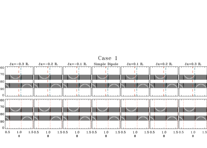
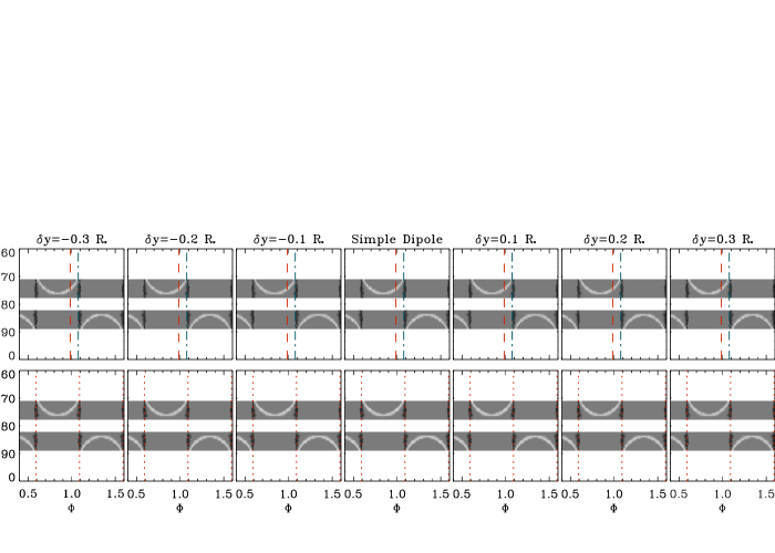
Figure 13: Simulations of the dynamical auroral light curves at the X and C bands (8.44 and 4.88 GHz respectively), similar to the simulations from a simple dipole shown in Fig. 4. The adopted sets of the model parameters are listed in Table 2. The auroral radio emission simulations here displayed explore the effects of the dipole shift along the $x$, $y$ and $z$-axes. The simulations shown in figure refer to the Case 1 described in Sec. 3.3.

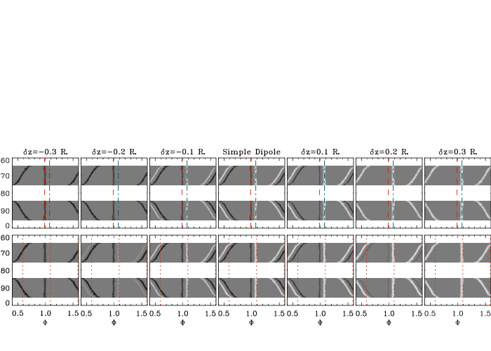
Figure 14: Same caption of Fig. 13, but simulations referred to the Case 2 described in Sec. 3.3.

References

- Antonova et al. (2008) Antonova A., Doyle J.G., Hallinan G., Bourke S., Golden A., 2008, A&A, 487, 317
- Antonova et al. (2013) Antonova A., Hallinan G., Doyle J.G., Yu S., Kuznetsov A., Metodieva Y., Golden A., Cruz K.L., 2013, A&A, 549, 131
- Babcock (1949) Babcock H.W., 1949, Observ. 69, 191
- Benz & Guedel (1994) Benz A.O., Guedel M., 1994, A&A, 285, 621
- Berger et al. (2001) Berger E., Ball S., Becker K.M., et al., 2001, Nature, 410, 338
- Berger (2002) Berger E., 2002, ApJ, 572, 503
- Berger (2006) Berger E., 2006, ApJ, 648, 629
- Berger et al. (2008a) Berger E., Gizis J.E., Giampapa M.S., et al., 2008a, ApJ, 673, 1080
- Berger et al. (2008b) Berger E., Basri G., Gizis J.E., et al., 2008b, ApJ, 676, 1307
- Berger et al. (2010) Berger E., Basri G., Fleming T.A., et al., 2010, ApJ, 709, 332
- Bonfond et al. (2012) Bonfond B., D. Grodent D., Gerard J.-C., et al., 2012, GeoRL, 39, 1105
- Burgasser & Putman (2005) Burgasser A.J., Putman M.E., 2005, ApJ, 626, 486
- Burgasser et al. (2015) Burgasser A.J., Melis C., Todd J., Gelino C.R., Hallinan G., Gagliuffi D.B., 2015, AJ, 150, 180
- Cecconi et al. (2012) Cecconi B., Hess S., Hérique A., et al., 2012, P&SS, 61, 32
- Chandra et al. (2015) Chandra P., Wade G.A., Sundqvist J.O., et al., 2015, MNRAS, 452, 1245
- Chabrier & Kuker (2006) Chabrier G, Kuker M., 2006, A&A, 446, 1027
- Clarke et al. (2002) Clarke J.T., Ajello J., Ballester G., et al., 2002, Nature, 415, 997
- Christensen et al. (2009) Christensen U.R., Holzwarth V., Reiners A., 2009, Nature, 457, 167
- Dahn et al. (2002) Dahn C.C., Harris H.C., Vrba F.J., et al., 2002, AJ, 124, 1170
- Donati et al. (2006) Donati J.-F., Forveille T., Collier Cameron A., et al., 2006, Sci, 311, 633
- Donati et al. (2008) Donati J.-F., Morin J., Petit P., et al., 2008, MNRAS, 390, 545
- Doyle et al. (2010) Doyle J.G., Antonova A., Marsh M.S., Hallinan G., Yu S., Golden A., 2010, A&A, 524, 15
- Drake et al. (1987) Drake S.A., Abbot D.C., Bastian T.S., Bieging J.H., Churchwell E., Dulk G., Linsky J.L, 1987, ApJ, 322, 902
- Ergun et al. (2000) Ergun R.E., Carlson C.W., McFadden J.P., Bieging J.H., Delroy G.T., 2000, ApJ, 538, 456
- Forbrich & Berger (2009) Forbrich J., Berger E., 2009, ApJ, 706, L205
- Forbrich et al. (2013) Forbrich J., Berger E., Reid M., 2013, ApJ, 777, 70
- Gawroński et al. (2017) Gawroński M.P., Goździewski K., Katarzyński K., 2017, MNRAS, 466, 4211
- Gillon et al. (2017) Gillon M., Triaud A.H.M.J., Demory B.-O., et al., 2017, Nature, 542, 456
- Gizis et al. (2016) Gizis J.E., Williams P.K.G., Burgasser A.J., et al., 2016, AJ, 152, 123
- Glagolevskij (2011) Glagolevskij Y.V., 2011, AstBu, 66, 144
- Guedel & Benz (1993) Guedel M., Benz A.O., 1993, ApJ, 405, L63
- Hallinan et al. (2006) Hallinan G., Antonova A., Doyle J.G., Bourke S., Brisken W.F., Golden A., 2006, ApJ, 653, 690
- Hallinan et al. (2007) Hallinan G., Bourke S., Lane C., et al., 2007, ApJ, 663, L25
- Hallinan et al. (2008) Hallinan G., Antonova A., Doyle J.G., Bourke S., Lane C., Golden A., 2008, ApJ, 684, 644
- Hallinan et al. (2015) Hallinan G., Littlefair S.P., Cotter G., et al., 2015, Nature, 523, 568
- Harding et al. (2013) Harding L.K., Hallinan G., Boyle R.P., Golden A., Singh N., Sheehan B., Zavala R.T., Butler R., 2013, ApJ, 779, 101
- Hatzes (1997) Hatzes A.P., 1997, MNRAS, 288, 153
- Hess et al. (2008) Hess S., Cecconi B., Zarka P., 2008, GeoRL, 35, L13107
- Hess et al. (2010) Hess S.L.G., Pétin, Zarka P., Bonfond B., Cecconi B., 2010, P&SS, 58, 1188
- Hess & Zarka (2011) Hess S., Zarka P., 2011, A&A, 531, 29
- Hess et al. (2011) Hess S., Bonfond B., Zarka P., Grodent D., 2011, J. Geophys. Res., 116, A05217
- Hill, Dessler & Michel (1974) Hill T.W, Dessler A.J., Michel F.C., 1974, GeoRL, 1, 3
- Hill (1979) Hill T.W, 1979, J. Geophys. Res, 84, 6554
- Jaeger et al. (2011) Jaeger T.R., Osten R.A., Lazio T.J., Kassim N., Mutel R.L., 2011, AJ, 142, 189
- Kao et al. (2016) Kao M.M., Hallinan G., Pineda J.S., Escala I., Burgasser A. Bourke S., Stevenson D., 2016, ApJ, 818, 24
- Kuker & Rudiger (1999) Kuker M., Rudiger G., 1999, A&A, 346, 922
- Kuznetsov et al. (2012) Kuznetsov A.A., Doyle J.G., Yu S., Hallinan G., Antonova A., Golden A., 2012, ApJ, 746, 99
- Lamy et al. (2008) Lamy L., Zarka P., Cecconi S., Hess S., Prangé, 2008, J. Geophys. Res., 113, A10213
- Lane et al. (2007) Lane C., Hallinan G., Zavala R.T., et al., 2007, ApJ, 668, L163
- Leone (1991) Leone F., 1991, A&A, 252, 198
- Leone & Umana (1993) Leone F., Umana G., 1993, A&A, 268, 667
- Leone et al. (1994) Leone F., Trigilio C., Umana G., 1994, A&A, 283, 908
- Leto et al. (2006) Leto P., Trigilio C., Buemi C.S., Umana G., Leone F., 2006, A&A, 458, 831
- Leto et al. (2012) Leto P., Trigilio C., Buemi C.S., Leone F., Umana G., 2012, MNRAS, 423, 1766
- Leto et al. (2016) Leto P., Trigilio C., Buemi C.S., Umana G., Ingallinera A., Cerrrigone L., 2016, MNRAS, 459, 1159 (Paper I)
- Leto et al. (2017) Leto P., Trigilio C., Oskinova L., et al., 2017, MNRAS, 467, 2820
- Lynch et al. (2015) Lynch C., Mutel R.L., Güdel M., 2015, ApJ, 802, 106
- Lynch et al. (2016) Lynch C., Murphy T., Ravi V., Hobbs G., Lo K., Ward C., 2016, MNRAS, 457, 1224
- Linsky et al. (1992) Linsky J.L., Drake S.A., Bastian S.A., 1992, ApJ, 393, 341
- Littlefair et al. (2008) Littlefair S.P., Dhillon V.S., Marsh T.R., Shahbaz T., Mart n E.L., Copperwheat C., 2008, MNRAS, 391, L88
- Lo et al. (2012) Lo K.K., Bray J.D., Hobbs G., et al., 2012, MNRAS, 421, 3316
- Louarn & Le Queau (1996a) Louarn P., Le Queau D., 1996a, P&SS, 44, 199
- Louarn & Le Queau (1996b) Louarn P., Le Queau D., 1996b, P&SS, 44, 211
- McLean et al. (2011) McLean M., Berger E., Irwin J., Forbrich J., Reiners A., 2011, ApJ, 741, 27
- McLean et al. (2012) McLean M., Berger E., Reiners A., 2012, ApJ, 746, 23
- Melrose & Dulk (1982) Melrose D.B., Dulk G.A., 1982, ApJ, 259, 844
- Menietti et al. (2011) Menietti J.D., Mutel R.L., Christopher I.W., Hutchinson K.A., Sigwarth J.B, 2011, J. Geophys. Res., 116, A12219
- Metodieva et al. (2017) Metodieva Y.T., Kuznetsov A.A., Antonova A.E., Doyle J.G., Ramsay G., Wu K., 2017, MNRAS, 465, 1995
- Mohanty & Basri (2003) Mohanty S., Basri G., 2003, ApJ, 583, 451
- Morin et al. (2008a) Morin J., Donati J.-F., Forville T., et al., 2008a, MNRAS, 384, 77
- Morin et al. (2008b) Morin J., Donati J.-F., Petit P., et al., 2008b, MNRAS, 390, 567
- Morin et al. (2010) Morin J., Donati J.-F., Petit P., et al., 2010, MNRAS, 407, 2269
- Mutel et al. (2008) Mutel R.L., Christopher I.W., Pickett J.S., 2008, GeoRL, 35, L07104.
- Nichols (2011) Nichols J.D., 2011, MNRAS, 414, 2125
- Nichols et al. (2012) Nichols J.D., Burleigh M.R., Casewell S.L., Cowley S.W.H., Wynn G.A., Clarke J.T., Westand A.A., 2012, ApJ, 760, 59
- Nichols & Milan (2016) Nichols J.D., Milan S.E., 2016, MNRAS, 461, 2353
- Oksala et al. (2012) Oksala M.E., Wade G.A., Townsend R.H.D., et al., 2012, MNRAS, 419, 959
- Oksala et al. (2015) Oksala M.E., Kochukhov O., Krticka J., et al., 2015, MNRAS, 451, 2015
- Osten et al. (2006) Osten R.A., Hawley S.L., Bastian T.S., Reid I.N., 2006, ApJ, 637, 518
- Queinnec & Zarke (1998) Queinnec J., Zarka P., 1998, J. Geophys. Res., 103, A11
- Ray & Hess (2008) Ray L.C., Hess S., 2008, J. Geophys. Res., 113, A11218
- Ravi et al. (2010) Ravi V., Hobbs G., Wickramasinghe D., Champion D.J., Keith M., 2010, MNRAS, 408, L99
- Reiners & Basri (2007) Reiners A., Basri G., 2007, ApJ, 656, 1121
- Reiners & Basri (2010) Reiners A., Basri G., 2010, ApJ, 710, 924
- Ricci et al. (2012) Ricci L., Testi L., Natta A., Scholz A., de Gregorio-Monsalvo I., 2012, ApJ, 761, L20
- Ricci et al. (2013) Ricci L., Isella A., Carpenter J.M., Testi L., 2013, ApJ, 764, L27
- Route & Wolszczan (2012) Route M., Wolszczan A., 2012, ApJ, 747, L22
- Route & Wolszczan (2013) Route M., Wolszczan A., 2013, ApJ, 773, 18
- Route & Wolszczan (2016) Route M., Wolszczan A., 2016, ApJ, 821, L21
- Route (2016) Route M., 2016, ApJ, 830, L27
- Schmidt et al. (2007) Schmidt S.J., Cruz K.L., Bongiorno B.J., Liebert J., Reid I.N., 2007, ApJ, 133, 2258
- Schrijver (2009) Schrijver C.J., 2009, ApJ, 773, L148
- Speir et al. (2014) Speir D.C., Bingham R., Cairns R.A., Vorgul I., Kellett B.J., Phelps A.D.R., Ronald K., 2014, Physical Review Letters, 113, 155002
- Tingay et al. (2013) Tingay S.J., Goeke R., Bowman J.D., et al., 2013, PASA, 30, e007
- Trigilio et al. (2000) Trigilio C., Leto P., Leone F., Umana G., Buemi C., 2000, A&A, 362, 281
- Trigilio et al. (2004) Trigilio C., Leto P., Umana G., Leone F., Buemi C.S., 2004, A&A, 418, 593
- Trigilio et al. (2008) Trigilio C., Leto P., Umana G., Buemi C.S., Leone F., 2008, MNRAS, 384, 1437
- Trigilio et al. (2011) Trigilio C., Leto P., Umana G., Buemi C.S., Leone F., 2011, ApJ, 739, L10
- van Haarlem et al. (2013) van Haarlem M.P., Wise M.W., Gunst A.W., et al., 2013, A&A, 556, A2
- Vorgul & Helling (2016) Vorgul I., Helling Ch., 2016, MNRAS, 458, 104
- Williams et al. (2014) Williams P.K.G., Cook B.A., Berger E., 2014, ApJ, 785, 9
- Williams et al. (2015a) Williams P.K.G., Berger E., Irwin J., Berta-Thompson Z.K., Charbonneau D., 2015, ApJ, 799, 192
- Williams et al. (2015b) Williams P.K.G., Casewell S.L., Stark C.R., Littlefair S.P., Helling Ch., Berger E., 2015, ApJ, 815, 64
- Williams & Berger (2015) Williams P.K.G., Berger E., 2015, ApJ, 808,189
- Williams et al. (2017) Williams P.K.G., Gizis J.E., Berger E., 2017, ApJ, 834, 117
- Winglee & Pritchett (1986) Winglee R.M., Pritchett P.L., 1986, J. Geophys. Res., 91, 13531
- Wolszczan & Route (2014) Wolszczan A., Route M., 2014, ApJ, 788, 23
- Wu & Lee (1979) Wu C.S., Lee L.C., 1979, ApJ, 230, 621
- Yadav et al. (2015) Yadav R.K., Christensen U.R., Morin J., Gastine T., Reiners A., Poppenhaeger K., Scott J.W., 2015, ApJ, 813, L31
- Yadav et al. (2016) Yadav R.K., Christensen U.R., Scott J.W., Poppenhaeger K., 2016, ApJ, 833, L28
- Yoneda et al. (2013) Yoneda M., Tsuchiya F., Misawa H., Bonfond C., Tao C., Kagitani M., Okano S., 2013, GeoRL, 40, 671
- Yu et al. (2011) Yu S., Hallinan G., Doyle J.G., et al., 2011, A&A, 525, A39
- Zarka (1998) Zarka P., 1998, J. Geophys. Res., 103, 20159
- Zarka (2007) Zarka P., 2007, P&SS, 55, 598