Multiscale modeling via split-step methods in neural firing

Abstract

Neuronal models based on the Hodgkin-Huxley equation form a fundamental framework in the field of computational neuroscience. While the neuronal state is often modeled deterministically, experimental recordings show stochastic fluctuations, presumably driven by molecular noise from the underlying microphysical conditions. In turn, the firing of individual neurons gives rise to an electric field in extracellular space, also thought to affect the firing pattern of nearby neurons.

We develop a multiscale model which combines a stochastic ion channel gating process taking place on the neuronal membrane, together with the propagation of an action potential along the neuronal structure. We also devise a numerical method relying on a split-step strategy which effectively couples these two processes and we experimentally test the feasibility of this approach. We finally also explain how the approach can be extended with Maxwell’s equations to allow the potential to be propagated in extracellular space.

Keywords: Computational neuroscience, Hodgkin-Huxley equation, Stochastic simulation, Multiphysics coupling, Lie-Trotter splitting.

AMS subject classification: 65C20, 92C20 (primary); 65C40, 65L99 (secondary).

1 Introduction

Neurons are responsible for encoding information in the central nervous system. Lower level functions are many times gathered at specific parts of the brain, processing information received from neurons throughout the body, often by means of signaling nerves, which are bundles of axons that reach out from the neurons. Higher level functions depend on remarkably larger and complex networks of neurons with various types of feedback loops.

The chemical connections between neurons are handled via synapses, where neurotransmitters are extruded into the extracellular space by the presynaptic neuron. The neurotransmitters form a part of a chemical process which may initiate a potential wave into the postsynaptic neuron — this wave is known as the action potential. During the action potential, the membrane potential quickly rises and falls, and the resulting signal propagates along the cell [29]. The process that underlies this propagation is the regulation of ion concentrations in both the intracellular cytoplasm and the extracellular space caused by integral membrane proteins called ion channels.

There are many variants of ion channel proteins, whose functions are only recently better understood through studies using experimental techniques such as X-ray crystallography [30]. To our current understanding, ion channels reside at one of many conformal states, which are either closed (non-conducting) or open (conducting). If the conformal state is open, ions are allowed to pass through pathways called pores from the extra- to the intracellular space, or in the opposite direction. If the conformal state is closed, ions are blocked from entering the channel [21]. Ion channels become activated either in response to a chemical ligand binding, or in response to voltage changes on the membrane [21, 29], so-called voltage-gated ion channels. In this work, we focus on voltage-gated ion channels, which are important for the initiation and the propagation of action potentials along the neuronal fiber.

Mathematical models of neurons were initially formed by measuring electrically induced responses of a neuron using techniques such as the voltage- or current clamp. From those experiments, transition properties and parameters of single channel gating could be identified [21].

Historically, models of firing neurons were formulated as ordinary differential equations (ODEs). However, in some specific cases experimental as well as theoretical findings suggest that the gating of ion channels is more accurately described by a stochastic process. The variance of the gating process, also known as the channel noise, is thought to be important for information processing in the dendrites and explain different phenomena regarding action potential initiation and propagation [32, 35, 15, 5]. For example, it has been shown that intrinsic noise is essential for the existence of subthreshold oscillations in stellate cells [10], that it contributes to irregular firing of cortical interneurons [33], and that it can explain firing correlation in auditory nerves [27].

Another important aspect of neuronal modeling is the investigation of action potentials propagating outward the neuron into the extracellular space. Simulations of such extracellular fields is one of the important methods used in computational neuroscience [12]. Common usage includes the validation of experimental methods such as EEG and extracellular spike recordings, or in the modeling of physiological phenomena which can not be easily investigated empirically [11].

In this paper we present a novel three-stage multiscale modeling framework consisting of the following components: (a) on the microscale, the gating process of the ion channels is governed by a continuous-time discrete-state Markov chain, (b) on the intermediate scale, the current-balance and the cable equation which are responsible for the action potential initiation and propagation is integrated in time as an ODE, (c) on the macroscale, the propagation of the trans-membrane current into an electrical field in extracellular space is achieved using partial differential equations (PDEs).

In §2 the three modeling layers are explained in some detail. The numerical method via split-step modeling is summarized in §3, where we also explain how the spatial coupling is achieved efficiently. We illustrate our method by some relevant examples in §4 and offer a concluding discussion in §5.

2 Neuronal modeling at different scales

We now describe the modeling framework at the individual scales, including the associated modeling assumptions. The microscale physics in the form of continuous-time Markov chains (CTMC) for the ion channels and the associated ion currents are discussed in §2.1, the ODE-model for the action potential along the neuronal geometry in §2.2, and the PDE-model of the extracellular electric field via Maxwell’s equations in §2.3. For convenience, a schematic explanation of the modeling framework is found in Figure 2.1.

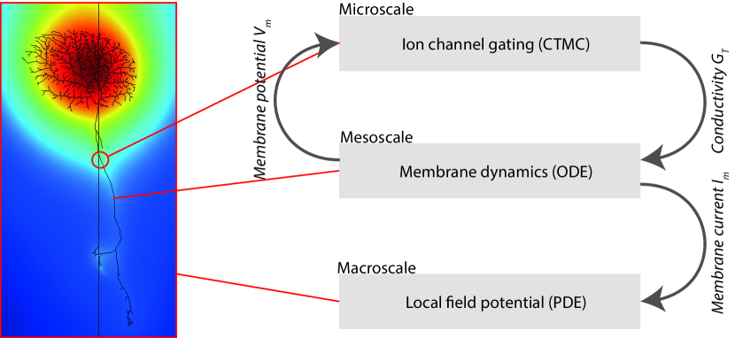
Figure 2.1: Schematic overview of the proposed multiscale modeling framework. The CTMC solution on the microscale depends on the membrane voltage that is computed on the mesoscale. This coupling is bidirectional; the mesoscale solution depends on the microscopic stochastic ion current. The macroscopic solution considered here depends solely on the mesoscopic membrane current.

2.1 Microscale: ion channel gating

The gating of voltage-dependent ion-channels is modeled by a Markov process. Hodgkin and Huxley [22] first proposed that the gating is governed by a set of gating variables. We assume that each gating variable takes values in a discrete state space and that a single combination of gating variables corresponds to an open and conducting ion channel [21].

$m_{0}h_{0}$ (A–B)¡=¿[$3\alpha_{m}$][$\beta_{m}$] $m_{1}h_{0}$ (B–C)¡=¿[$2\alpha_{m}$][$2\beta_{m}$] $m_{2}h_{0}$ (C–D)¡=¿[$\alpha_{m}$][$3\beta_{m}$] $m_{3}h_{0}$ (@A–E)¡=¿[$\alpha_{h}$][$\beta_{h}$][-90] $m_{0}h_{1}$ (@B–F)¡=¿[$\alpha_{h}$][$\beta_{h}$][-90] $m_{1}h_{1}$ (@C–G)¡=¿[$\alpha_{h}$][$\beta_{h}$][-90] $m_{2}h_{1}$ (@D–H)¡=¿[$\alpha_{h}$][$\beta_{h}$][-90] $\mathbf{m_{3}h_{1}}$ (@E–@F)¡=¿[$3\alpha_{m}$][$\beta_{m}$] (@F–@G)¡=¿[$2\alpha_{m}$][$2\beta_{m}$] (@G–@H)¡=¿[$\alpha_{m}$][$3\beta_{m}$]

Figure 2.2: Kinetic scheme for the $m_{3}h_{1}$ sodium channel gating proposed by Hodgkin and Huxley [22]. Only the gating state $m_{3}h_{1}$ represents an open ion channel, for all other states the ion channel is closed.

The gating states and the transitions between them can be written in the form of a kinetic scheme. An example for the voltage-gated $m_{3}h_{1}$ sodium channel is depicted in Figure 2.2. The notation for the channel states indicates that there are two involved gating variables $m$ and $h$, where variable $m$ takes one of four states and, independently, variable $h$ takes one of two states. In total we thus arrive at 8 states with a total of 10 reversible transitions, see Figure 2.2. The total number of channels in the open state $m_{3}h_{1}$ implies a certain conductivity as will be detailed below. The transition rates between the states depend on the membrane voltage and on the state itself. When these transitions take place in a microscopic environment where molecular noise is present, a continuous-time Markov chain (CTMC) is the most suitable model.

$S_{1}$ (A–B)¡=¿ $S_{2}$ (B–C)¡=¿ $S_{3}$ (C–D)¡=¿ $S_{4}$ (@A–E)¡=¿[-90] $S_{5}$ (@B–F)¡=¿[-90] $S_{6}$ (@C–G)¡=¿[-90] $S_{7}$ (@D–H)¡=¿[-90] $\mathbf{S_{8}}$ (@E–@F)¡=¿ (@F–@G)¡=¿ (@G–@H)¡=¿

Figure 2.3: An equivalent scheme to Figure 2.2, where each combination of gating variables corresponds to a discrete state of a Markov chain.

We rewrite such schemes in a general, yet more manageable notation as follows. Assign the different combinations of gating variables an individual state $S_{i}$, $i=1,2,\ldots,M_{\mbox{\scriptsize{states}}}$. For the sodium scheme in Figure 2.2 there are 8 states and only the state $S_{8}$ corresponds to an open and conducting ion channel. The resulting equivalent scheme is shown in Figure 2.3 and an exemplary set of transitions and rates is

$$S_{3} \longrightarrow S_{4}\text{, rate: }\alpha_{m}(V_{m}),$$ (2.1)

$$S_{3} \longrightarrow S_{2}\text{, rate: }2\beta_{m}(V_{m}),$$ (2.2)

$$S_{3} \longrightarrow S_{7}\text{, rate: }\alpha_{h}(V_{m}),$$ (2.3)

where $V_{m}$ is the membrane potential at the location of the ion channel. For this particular example, the transition rates used by Hodgkin and Huxley are [22]

$$\alpha_{m}(V_{m}) =\frac{0.1(V_{m}+40)}{1-e^{-(V_{m}+40)/10}},$$ (2.4)

$$\beta_{m}(V_{m}) =4e^{-(V_{m}+65)/18},$$ (2.5)

$$\alpha_{h}(V_{m}) =0.07e^{-(V_{m}+65)/20},$$ (2.6)

$$\beta_{h}(V_{m}) =\frac{1}{1+e^{-(V_{m}+35)/10}}.$$ (2.7)

The rates (2.4)–(2.7) were originally obtained by empirical fitting to experimental data and are formulated relative to the resting potential of the particular neuron model. We consider a small neural compartment $a$, obtained from a discretization of the neuronal fiber into small enough segments such that the potential is approximately constant within each compartment. Let there be a total of $N^{a}$ ion channels of the considered type (e.g. the $m_{3}h_{1}$ sodium channel) on the compartmental surface. At any instant in time $t$, let $s_{i}$ be the number of channels in state $S_{i}$, $i=1,2,\ldots,M_{\mbox{\scriptsize{states}}}$. The scheme in Figure 2.3 now directly translates into Markovian transition rules for the states $s\in\mathbf{Z}_{+}^{8}$, i.e. the ion-channel counts, thus defining a CTMC $(t,s)\in\mathbf{R}_{+}\times\mathbf{Z}_{+}^{8}$.

To model the electrophysiological properties of the ion channel, we define the single open channel conductance $\gamma$, as well as the neuronal membrane area $A^{a}$ such that the area density of ion channels is $\varrho^{a}=N^{a}/A^{a}$. If $O^{a}$ is the count of the open ion channels, e.g., for the above example this is $O^{a}=S^{a}_{8}$, we arrive at the total conductance

$$G^{a}=\frac{O^{a}}{N^{a}}\varrho^{a}A^{a}\gamma.$$ (2.8)

Next, the trans-membrane current produced by the ion channel is given by Ohm’s law,

$$I^{a}=G^{a}(V^{a}_{m}-E),$$ (2.9)

where $E$ is the reverse potential of the ion channel, that is, the membrane potential under which the trans-membrane current $I^{a}$ is zero, and where $V^{a}_{m}$ is the membrane potential in compartment $a$.

In the macroscopic setting proposed by Hodgkin and Huxley [22], the transitions between the gating states happened according to first order reaction kinetics. The fraction of closed channels $(1-o^{a})$ becomes open with rate $\alpha$ and the fraction of open channels $o^{a}$ becomes closed with rate $\beta$. Note that $\alpha$ and $\beta$ may be voltage-dependent for specific types of ion-channels, as in (2.1)–(2.7). The resulting ODE for each macroscopic gating variable $o^{a}$ can then be written as

$$\frac{do^{a}}{dt}=\alpha(1-o^{a})-\beta o^{a}.$$ (2.10)

Under the macroscopic formulation, the ratio of open channels is approximated as

$$\frac{O^{a}}{N^{a}}\approx\prod_{i=1}^{M}\limits[o^{a}_{i}]^{p_{i}},$$ (2.11)

where $M$ is the number of gating particles for the particular ion channel model, and $p_{i}$ is the exponent of the $i$th gating variable $o_{i}$.

As a concrete example, the sodium channel $m_{3}h_{1}$ depicted in Figure 2.2 is gated by gating variables $m$ and $h$, which in the macroscopic formulation have an exponent of three and one, respectively. In relation to (2.11) this means that $o_{1}=m$ with $p_{1}=3$, and $o_{2}=h$ with $p_{2}=1$, where $m$ and $h$ are here just symbols denoting the concentration of the gating variables. The ratio of open channels is then approximated as

$$\frac{O_{Na}}{N_{Na}}\approx m^{3}h^{1},$$ (2.12)

and the deterministic gating function for each variable obeys

$$\frac{dm}{dt} =\alpha_{m}(1-m)-\beta_{m}m,$$ (2.13)

$$\frac{dh}{dt} =\alpha_{h}(1-h)-\beta_{h}h,$$ (2.14)

where $\alpha$ and $\beta$ are the voltage dependent transition rates defined in (2.4)–(2.7). Solving (2.13)–(2.14) and using (2.9) thus constitutes the classical Hodgkin-Huxley ODE model for the ionic current. By rather evolving the Markov chain defined implicitly in Figure 2.3 and using (2.8)–(2.9), a stochastic current is defined. This stochastic model is the result of the microphysical assumption of discrete ion states obeying Markovian (memoryless) transition rules. For large enough numbers of ion channels, a transition into the corresponding deterministic model can be expected under rather broad conditions [14]. When a fine enough compartmentalization of a particular neuron is made, however, the stochastic model can be expected to be more realistic in the sense that the effects missing in a corresponding deterministic model can not be ignored.

We now proceed to discuss the appropriate model for evolving the resulting current, be it stochastic or deterministic, over the neuronal morphology.

2.2 Intermediate scale: current-balance and cable equation

On the intermediate scale, we solve for the current-balance equation of the neuron, describing the relation between the membrane voltage and the different current sources. We first take the ionic current sources from the microscale into account. We next model the capacitance of the membrane, a so-called passive neuronal property. As the neuronal morphology is divided into several compartments we also include a term for the propagation of voltage between the compartments, resembling the cable equation.

As before, denote the compartments by the index $a\in\{1,\ldots,M_{\mbox{\scriptsize{compartments}}}\}$. For each connection between compartments, an entry is made in the adjacency matrix $\mathcal{A}$ [9]. Typically, a compartment is connected to two or three neighbors. If a compartment is connected to only a single neighbor, it represents one of the end-points of the neuron. An example is found in Figure 2.4.

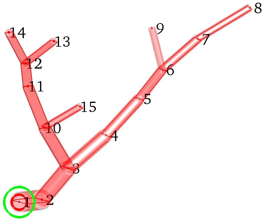
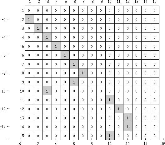
Figure 2.4: Geometry of a neuron and the associated adjacency matrix $\mathcal{A}$ (figure adapted from [9]). A nonzero entry in $\mathcal{A}$ implies a connection between the corresponding compartments.

The current flowing in each compartment is composed from different components. The current source of compartment $a$ is the total axial current with respect to its connected compartments $b\in\mathcal{B}(a)$. Note that as $\mathcal{A}$ represents a directed graph, the connected component $b\in\mathcal{B}(a)$ represents in-neighbors that are connected via an edge in the direction to vertex $a$, as well as out-neighbors which are connected by an edge outwards of vertex $a$. According to Ohm’s law the current equals

$$I^{a}_{axial}=\sum_{b\in\mathcal{B}(a)}G^{a}_{b}(V^{a}_{m}-V^{b}_{m})=\sum_{b\in\mathcal{B}(a)}G^{a}_{b}V^{a}_{m}-\sum_{b\in\mathcal{B}(a)}G^{a}_{b}V^{b}_{m},$$ (2.15)

where $G^{a}_{b}$ is the conductance between compartments $a$ and $b$, and where $V^{a}_{m}$ is the trans-membrane potential of compartment $a$.

We then add the ionic currents computed at the microscale. For the sake of generality we extend the previous notation of a single type of ion channel into $c$ types, $\mathcal{T}=\{T^{1},\ldots,T^{c}\}$, acting simultaneously. Generalizing (2.9) we arrive at the total ionic current

$$I^{a}_{ionic}=\sum_{T}G^{a}_{T}(V^{a}_{m}-E_{T}).$$ (2.16)

We now deviate slightly from the discussion and first consider a space-continuous solution obtained by solving for the propagation of the potential on a line oriented along the $x$-axis. Adding the axial current flux $I_{axial}$, the total trans-membrane current flux $I_{m}$, and a possibly additional external current source $I_{inj}$ gives

$$C_{m}\frac{d}{dt}V_{m} =I_{inj}-I_{m}-I_{axial},$$ (2.17)

where $C_{m}$ is the capacitance of the neuronal membrane. We have that the gradient of the inter-compartmental leakage current $I_{L}$ is

$$\frac{\partial I_{L}}{\partial x}=-I_{m}.$$ (2.18)

The leakage current accounts for the ions that diffuse out of the intracellular space due to the natural permeability of the neuronal membrane.

Given a suitable resting potential, Ohm’s law is

$$I_{L}=G_{L}\frac{\partial V_{m}}{\partial x}.$$ (2.19)

Substituting $I_{m}$ from (2.17) using (2.18)–(2.19), we get what is commonly referred to as the cable equation,

$$G_{L}\frac{\partial^{2}V_{m}}{\partial x^{2}}=C_{m}\frac{\partial V_{m}}{\partial t}-I_{inj}+I_{axial}.$$ (2.20)

Given the parabolic character of this equation, the Crank-Nicholson scheme [8] is a natural choice when designing numerical methods.

Turning now to the compartment-discrete version, the leakage current in each compartment $a$ is given as

$$I^{a}_{L}=G^{a}_{L}(V^{a}_{m}-E^{a}_{L}),$$ (2.21)

where the membrane leakage conductivity $G^{a}_{L}$ and the leak reverse potential $E^{a}_{L}$ are regarded as constants.

The total trans-membrane current flux now becomes

$$I^{a}_{m}=I^{a}_{L}+I^{a}_{ionic}=(G^{a}_{L}+\sum_{T}G^{a}_{T})V^{a}_{m}-(G^{a}_{L}E^{a}_{L}+\sum_{T}G^{a}_{T}E_{T}).$$ (2.22)

In order to solve for the membrane potential in each compartment $a$, we start from a discrete version of (2.17), using (2.15) and (2.22),

$$C^{a}_{m}\frac{d}{dt}V^{a}_{m} =I^{a}_{inj}-I^{a}_{m}-I^{a}_{axial}=I^{a}_{inj}-(I^{a}_{L}+\sum_{T}I^{a}_{T})-I^{a}_{axial}$$ (2.23)

$$=I^{a}_{inj}+(G^{a}_{L}E^{a}_{L}+\sum_{T}G^{a}_{T}E_{T})-(G^{a}_{L}+\sum_{T}G^{a}_{T})V^{a}_{m}$$

$$\phantom{=}-\sum_{b}G^{a}_{b}V^{a}_{m}+\sum_{b}G^{a}_{b}V^{b}_{m}.$$ (2.24)

To summarize, on the intermediate scale we insert the stochastic conductivity $G^{a}_{T}$ computed from (2.8) into (2.16) and solve the current-balance equation (2.23) for each of the neural compartments. We simultaneously solve for the trans-membrane current defined in (2.22), to be coupled into the macroscopic field — next to be discussed.

2.3 Macroscale: extracellular field potentials

To simulate spatially non-homogeneous distributions of electrical fields produced by single neurons and neuronal networks, we use an electrostatic formulation of Maxwell’s equations to be discretized with finite elements. We solve for the electric field intensity $\mathbf{E}$ in terms of the electric scalar potential $V$,

$$\mathbf{E}=-\nabla V.$$ (2.25)

The relevant dynamic form of the continuity equation with current sources $Q_{j}$ is given by

$$\nabla\cdot\mathbf{J}=-\frac{\partial\rho}{\partial t}+Q_{j},$$ (2.26)

with $\mathbf{J}$ and $\rho$ the current density and electric charge density, respectively. Further constitutive relations include

$$\mathbf{D}=\varepsilon_{0}\varepsilon_{r}\mathbf{E},$$ (2.27)

and Ohm’s law

$$\mathbf{J}=\sigma\mathbf{E},$$ (2.28)

in which $\mathbf{D}$ denotes the electric flux density. Finally, Gauss’ law states that

$$\nabla\cdot\mathbf{D}=\rho.$$ (2.29)

Upon taking the divergence of (2.28) and using the continuity equation (2.26) we get

$$\nabla\cdot(\sigma\mathbf{E})=-\frac{\partial\rho}{\partial t}+Q_{j}.$$ (2.30)

Rewriting the electric charge density using Gauss’ law together with the constitutive relation (2.27) and finally applying the gauge condition (2.25) twice we arrive at the time-dependent potential formulation

$$-\nabla\cdot\left(\sigma\nabla V+\varepsilon_{0}\varepsilon_{r}\frac{\partial}{\partial t}\nabla V\right)=Q_{j}.$$ (2.31)

The values for the electric conductivity $\sigma$ and the relative permittivity $\varepsilon_{r}$ were obtained from [2]. The source currents $Q_{j}$ are computed from the compartmental model described in §2.2. Specifically, in compartment $a$, we put

$$Q_{j}(t) =\frac{I_{m}^{a}(t)}{A^{a}},$$ (2.32)

where $I_{m}^{a}(t)$ is obtained by solving (2.22) and where we recall that $A^{a}$ is the area of the neuronal membrane in compartment $a$.

The boundary conditions here are homogeneous Neumann conditions (electric isolation) everywhere except in a single point which we take to be ground ($V=0$). In all our simulations this point was placed at the axis of rotation of the enclosing cylindrical extracellular space, and directly underneath the neuronal geometry. This procedure ensures that the formulation has a unique solution; without this specification it is otherwise only specified up to a constant.

3 Numerical modeling

The processes at the three scales, that is, the microphysics of the ion channel gating, the neuron current at the intermediate scale, and the propagation of the electric field, all take place in continuous time. Also, all processes formally affect eachother through two-way couplings.

In §3.1 we discuss the numerical coupling of the ion channel gating and the cable equation via a split-step strategy. In §3.2 the propagation of the electric potential into extracellular space is summarized and here we also explain how the often rather complicated neuronal geometry is handled. To simplify matters, we will disregard the usually much weaker coupling from the external electric field back to the gating process.

3.1 Numerical coupling of firing processes

To get to grip with the details of the coupling between the ion channel gating process and the propagation of the action potential along the neuron we need a more compact notation as follows. In compartment $a$, denote by $\mathbb{X}^{a}(t)$ the gating state, that is, the number of channels being in each of the different states at time $t$. For our sodium channel example we have $\mathbb{X}^{a}(t)=[s_{1}^{a},s_{2}^{a},\ldots,s_{8}^{a}](t)^{T}$. The CTMC may be written compactly as

$$d\mathbb{X}^{a}(t) =\mathbb{S}\boldsymbol{\mu}^{a}(\mathbb{X}^{a},V_{m}^{a};\,dt),$$ (3.1)

for $$a=1,\ldots,M_{\mbox{\scriptsize{compartments}}} \mathbb{S} M_{\mbox{\scriptsize{states}}}\times N_{\mbox{\scriptsize{transitions}}} (\mathbb{X}^{a},V_{m}^{a}) \boldsymbol{\mu}^{a} N_{\mbox{\scriptsize{transitions}}} S_{3}\longrightarrow S_{4}$$, and where is an matrix of integer transition coefficients. The dependency on the state is implicit in the random counting measure associated with an -dimensional Poisson process. As a concrete example, the transition in (2.1) satisfies

$$\mathbb{E}[\boldsymbol{\mu}^{a}_{i}(\mathbb{X}^{a},V_{m}^{a};\,dt)] =\mathbb{E}[\mathbb{X}^{a}_{3}\,\alpha_{m}(V_{m}^{a})]\,dt,$$ (3.2)

with

$$\mathbb{S}_{3,i}=-\mathbb{S}_{4,i}=-1,$$ (3.3)

that is, with the understanding that (2.1) is the $i$th transition according to some given ordering. Since the process is a Poisson process, (3.2) expresses independent exponentially distributed waiting times of intensity $\alpha_{m}(V_{m}^{a})$ for each of the $\mathbb{X}^{a}_{3}$ possible transitions of type $S_{3}\longrightarrow S_{4}$.

The propagation of the action potential can similarly be written in more compact ODE notation,

$$dV_{m}^{a}(t) =G(\mathbb{X}^{a},V_{m}^{a},\{V_{m}^{b}\}_{b\in\mathcal{B}(a)})\,dt,$$ (3.4)

where $G$ is just the current-balance equation (2.23) and which depends on the state $(\mathbb{X}^{a},V_{m}^{a})$ via (2.8), (2.16), and (2.22), respectively.

Eqs. (3.1) and (3.4) form a coupled CTMC-ODE model which falls under the scope of Piecewise Deterministic Markov Processes (PDMPs) and for which numerical methods have been investigated [31]. A highly accurate implementation is possible through event-detection in traditional ODE-solvers. This, however, has a performance drawback since the ODE-solver must continuously determine to sufficient accuracy what micro-event happens when. In the experiments in §4 we have chosen to rely on a simple split-step strategy as follows. Given a discrete time-step $\Delta t$, and $t_{n+1}=t_{n}+\Delta t$,

$$\mathbb{X}^{a}_{n+1} =\mathbb{X}^{a}_{n}+\int_{t_{n}}^{t_{n+1}}\mathbb{S}\boldsymbol{\mu}^{a}(\mathbb{X}^{a}(s),V_{m,n}^{a};\,ds),$$ (3.5)

$$V_{m,n+1}^{a} =V_{m,n}^{a}+\int_{t_{n}}^{t_{n+1}}G(\mathbb{X}^{a}_{n+1},V_{m}^{a}(s),\{V_{m}^{b}(s)\}_{b\in\mathcal{B}(a)})\,ds.$$ (3.6)

That is, (3.5) evolves the CTMC (3.1) keeping the voltage potential fixed at its value from the previous time-step $t_{n}$. Similarly, (3.6) evolves the ODE (3.4) while keeping the state of the ion channels fixed at the time-step $t_{n+1}$. Importantly, the usually more expensive stochastic simulation in (3.5) is fully decoupled as it only depends on the state of the compartment $a$. The global step is achieved separately by solving the connected ODE in (3.6), and is usually quite fast.

The approximation (3.5)–(3.6) can be understood as a split-step method and may also be analyzed as such [13, 6]. The order of the approximation can then be expected to be $1/2$ in the root mean-square sense,

$$\mathbb{E}[\|\mathbb{X}_{n}-\mathbb{X}(t_{n})\|^{2}+\|V_{m,n}-V_{m}(t_{n})\|^{2}]\leq C\Delta t.$$ (3.7)

Although it appears to be difficult to increase the stochastic order of this approximation, the accuracy is likely going to increase by turning to symmetric Strang-type splitting methods for the stochastic part [13], possibly also adopting a higher order scheme for the ODE-part. However, the efficiency of such an approach ultimately depends on the strength of the nonlinear feedback terms and is difficult to analyze a priori. In the present proof-of-concept context we aim at a convergent and consistent coupling for which (3.5)–(3.6) are a suitable starting point. We thus postpone the investigation of more advanced integration methods for another occasion.

3.2 Spatial extension of the firing process

The modeling in §2.2 did not take into account a possible free-space potential $V_{ext}$, external to the cell. The necessary modifications to incorporate this are as follows. For $x\in\Omega\subset\mathbf{R}^{3}$, let $V_{ext}(x)$ be a given external potential and denote by $V_{ext}^{a}$ the value at compartment $a$. Then replace (2.23) with

$$I^{a}_{m} =I^{a}_{L}+I^{a}_{ionic}+I^{a}_{ext}$$ (3.8)

$$=(G^{a}_{L}+\sum_{T}G^{a}_{T})V^{a}_{m}-(G^{a}_{L}E^{a}_{L}+\sum_{T}G^{a}_{T}E_{T})+G^{a}_{m}V^{a}_{ext}.$$

for $G^{a}_{m}$ the membrane transneuronal conductivity. With this modification, (2.23) propagates the effect of the given external field $V_{ext}(x)$ along the neuron.

In §2.3 we discussed how the effect of a trans-membrane current propagates into extracellular space as an electric potential $V$ (cf. (2.31)–(2.32)). With the previous discussion in mind, the following two-way coupling thus emerges: the solution of the current-balance equation (2.23) yields a current source, which feeds into (2.32). In turn, this implies an external potential $V_{ext}:=V$, obtained by solving (2.31), finally to be inserted into (3.8) above. The full model coupling thus arrived at takes the schematic form

$$\mbox{\S\ref{sec:microscale}}\xrightleftharpoons{\hphantom{MM}}\mbox{\S\ref{sec:mesoscale}}\xrightleftharpoons{\hphantom{MM}}\mbox{\S\ref{sec:macroscale}}.$$ (3.9)

It is certainly possible to devise a numerical method using a similar split-step strategy as in §3.1 for this full coupling. As mentioned before, to simplify we shall assume that the feedback from the external field and onto the neuron is weak, such that $V_{ext}\approx 0$ in (3.8) and we thus consider the simplified model (see also Figure 2.1)

$$\mbox{\S\ref{sec:microscale}}\xrightleftharpoons{\hphantom{MM}}\mbox{\S\ref{sec:mesoscale}}\xrightarrow{\hphantom{MM}}\mbox{\S\ref{sec:macroscale}}.$$ (3.10)

This assumption is valid whenever the simulation consists of a small number of neighboring neurons, but becomes inaccurate if a large number of nearly parallel neurons is considered. See [1, 4] for a further discussion. It follows that the solution of the field potential $V$ can be done “offline”. That is, this problem may be solved in isolation using a pre-recorded current source $I_{m}^{a}(t)$ obtained from the split-step method described in §3.1.

The three-dimensional neuronal geometry was constructed in Comsol Multiphysics with the help of the interface to Matlab (“LiveLink”) by morphological additions and Boolean unification of simple geometric objects, representing neuronal compartments. The TREES Toolbox [9] was used to conveniently access the geometrical properties of single compartments over the Matlab interface. More specifically, the geometry was constructed by parsing the adjacency graph $\mathcal{A}$. Starting from the initial node of the graph, this procedure makes sure that each compartment is connected to the same neighbors as in the numerical model for the axial current flow in (2.15).

In an initial attempt, we aimed to represent the 3D geometry as an exact counterpart of the compartmental model, where each compartment is understood as a cylinder with a certain length and diameter. If the direction of the main axes of any two joining cylinders differed, a sphere was added in between the cylinders, followed by a removal of all interior boundaries. Although this created a direct volumetric representation of the neuronal compartments, the approach is difficult to generalize to neuronal branches with a more complicated connectivity. The reason is that the triangulation of the final object becomes extremely difficult to achieve as the mesh engine insists on fully resolving the curvature. See Figure 3.1 for an example of a problematic mesh, emerging at the intersection of a cylinder and a sphere.

A second and more successful attempt was made by which three-dimensional curves made up of line segments for each compartment was constructed. This simplifies the meshing process immensely, since the extracellular mesh is not constrained by high-curvature cylindrical boundaries. Implicit here is the assumption that the neuron is very thin compared to the external length-scale of practical interest. This is valid as the diameter of a dendritic structure is $\approx 1\mu m$ and the considered extracellular space is typically in the range of several $mm$ [12]. In Figure 3.2 we show examples of both approaches.

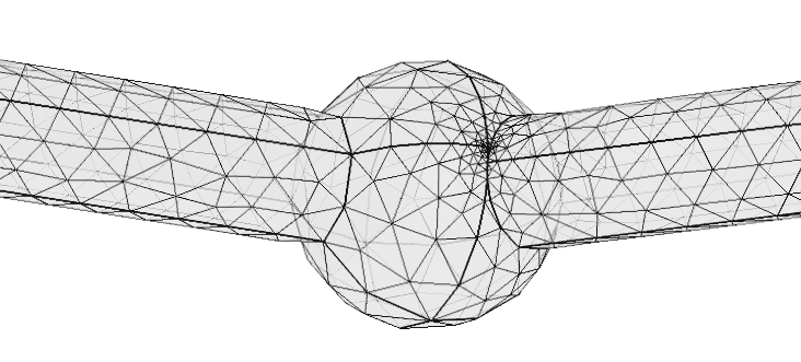
Figure 3.1: Example of a problematic mesh at the intersection of two cylindrical compartments.

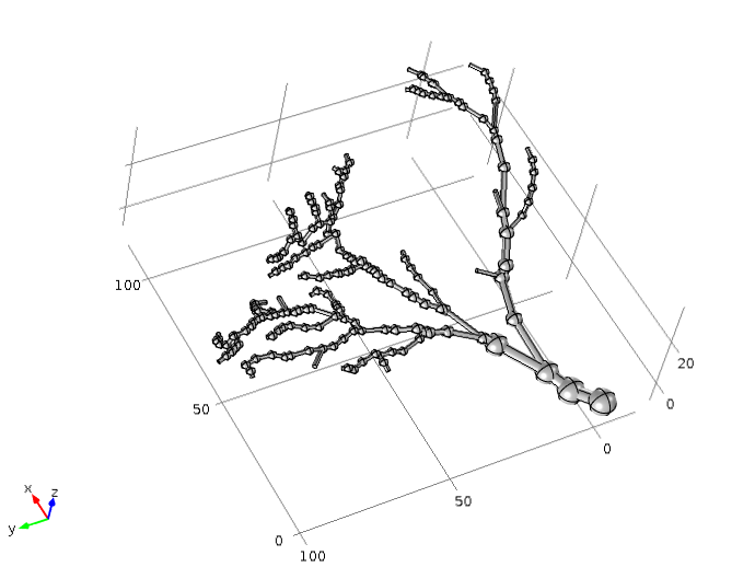
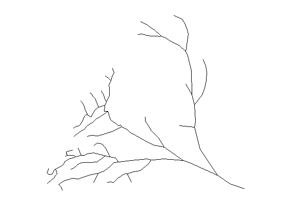
Figure 3.2: Example of a neuronal morphology created with cylindrical objects (left), and with curves (right).

4 Experiments

We devote this section to some feasibility experiments of the method proposed. In §4.1 we look in some detail at the coupling of the microscopic and intermediate scales. Using the stochastic currents so computed, the induced electrical field is propagated outside the neuron in §4.2.

4.1 Micro-meso coupling

In this section we provide numerical experiments of the coupling between the microscopic scale, introduced in §2.1, and the mesoscopic scale, introduced in §2.2. We simulate the classical squid model proposed by Hodgkin and Huxley [22], which is also a part of a widely used benchmark for neuronal simulators [3]. The model includes two types of voltage-gated ion channels, $Na^{+}$ and $K^{+}$ ions, which in our case are both modeled as continuous-time Markov processes (cf. §2.1). The kinetic gating scheme for the $Na^{+}$ channel is shown in Figure 2.2. The $K^{+}$ channel follows a similar scheme, but has only four discrete gating states $S_{1},\ldots,S_{4}$, of which only the state $S_{4}$ is open. The transition rates in this case are voltage-dependent as follows [22]

$$\alpha_{n}(V_{m}) =\frac{0.01(V_{m}+10)}{e^{(V_{m}+10)/10}-1},$$ (4.1)

$$\beta_{n}(V_{m}) =0.125e^{(V_{m}/80)}.$$ (4.2)

Note the similar form of (4.1) to (2.4) and (4.2) to (2.5), respectively, which is due to using the same empirical fitting procedure. The density of the ion channels is $\varrho_{K}=30\leavevmode\nobreak\ \mu$m^-2 and $\varrho_{Na}=330\leavevmode\nobreak\ \mu$m^-2, respectively [21]. The single channel conductance equals $\gamma^{K}=360/30\leavevmode\nobreak\ pS$, and $\gamma^{Na}=1200/330\leavevmode\nobreak\ pS$, while the reversal potentials are $E_{K}=-77\leavevmode\nobreak\ mV$ and $E_{Na}=50\leavevmode\nobreak\ mV$ [3].

The parameters for the intermediate scale are as follows. The specific membrane capacitance $c_{m}=1\mu F(cm)^{-2}$, resting potential $E_{r}=-65\leavevmode\nobreak\ mV$, cytoplasm resistivity $\varrho_{c}=100\leavevmode\nobreak\ \Omega cm$, specific leak conductance $g_{L}=40000^{-1}\leavevmode\nobreak\ S(cm)^{-2}$ and leak reversal potential $E_{L}=-65\leavevmode\nobreak\ mV$ [3]. We let the model be confined to a cylindrical geometry with a length of $1\leavevmode\nobreak\ mm$ and a diameter of $1\leavevmode\nobreak\ \mu m$. The cylinder is compartmentalized into $M_{\mbox{\scriptsize{compartments}}}$ sub-cylinders of equal length and diameter. The root node is ignited by a current injection of $0.1\leavevmode\nobreak\ nA$.

In practice we use the Gillespie’s “Direct Method” [17] to evolve (3.5) and the Crank-Nicholson scheme [8] to solve (3.6), relying on the fact that the latter is linear in $V_{m}^{a}$.

In Figure 4.1 we show the numerical solution of the coupled model, overlaid with the deterministic solution where ion channels are described by ODEs as in (2.13)–(2.14). We show three traces of the membrane voltage $V_{m}$ in one neuronal compartment over time, where the injected current has been varied from a lower value ($0.045nA$) to a larger value ($0.1nA$). The dynamics of the stochastic model for the initial current injections clearly differ from the dynamics of the deterministic one, where a single spike or a train of spikes can be triggered in the stochastic representation, while no spike can be obtained in the deterministic one. At the higher amount of current injection, we observe a trace with similar characteristics for both model representations, but with an increasingly different phase shift.

In Figure 4.2 we show a numerical convergence study of the coupled model, concerning two method parameters. We show how the interspike interval (ISI) changes as a function of the coupling time step $\Delta t$, as well as the discretization of the geometry $\Delta x$. The ISI is defined as the duration between the peaks of two spikes. As the neuronal firing is now a stochastic process, the ISI will be a distribution, and hence we present the first and second moments. We find that, for the study of the coupling time step, the ISI appears to be well resolved at $\Delta t=10^{-1}\leavevmode\nobreak\ ms$ for the spatial discretization presented. For the spatial discretization, we find that the ISI distributions do not significantly differ for a voxel length of under 1$\mu m$.

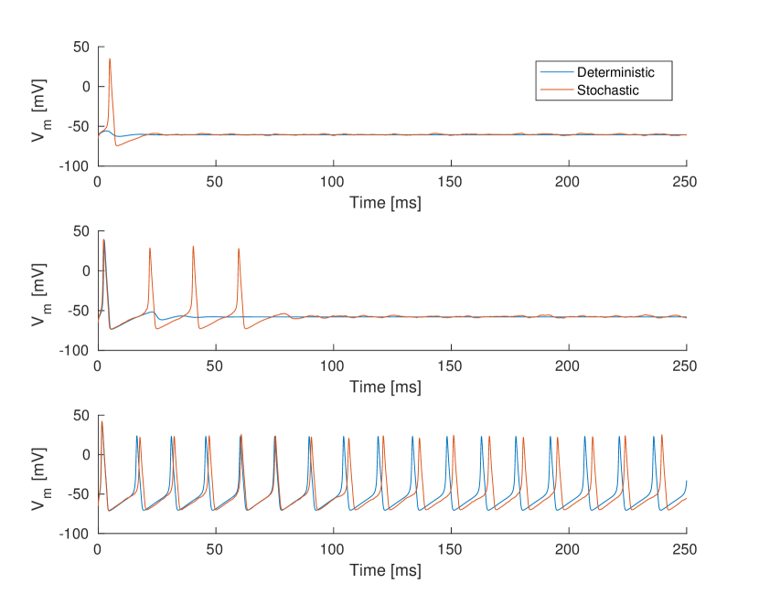
Figure 4.1: Membrane voltage behavior around threshold current. The accuracy of the deterministic solver was verified with the reference solution of Rallpack 3. In all cases the discretization is $\Delta t=0.05$ and $\Delta x=0.05$. Upper: injected current is $I_{inj}=0.045$ $nA$, middle: injected current is $I_{inj}=0.063$ $nA$, lower: injected current is $I_{inj}=0.1$ $nA$.

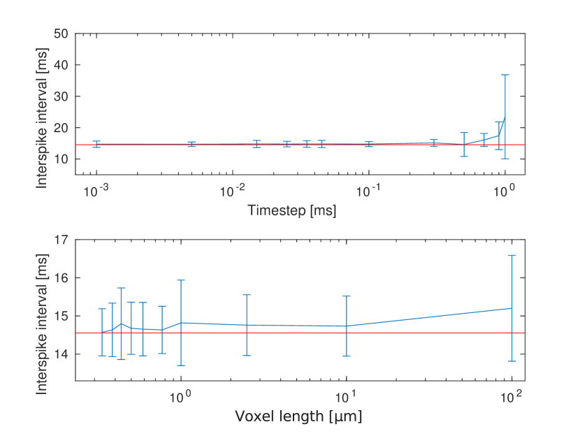
Figure 4.2: Top: The mean interspike interval (ISI) $\pm$ standard error as a function of the time step $\Delta t$. The compartment length is here $\Delta x=0.02$. Bottom: The ISI as a function of the compartment length $\Delta x$ at a time step $\Delta t=0.05$. The red line represents the interspike interval from the Rallpack 3 reference solution [3]. The number of trajectories in all runs is $N=40$.

4.2 Three-scale coupling

For this example we took the morphological description of a pyramidal CA1 neuron from [28], which contains about 1500 compartments. We re-sampled the geometry in order to aggregate short compartments of sizes less than $50\leavevmode\nobreak\ \mu m$ into larger compartments, leading to a final representation consisting of approximately 400 compartments. Although the reduction might alter the properties of the model and more evolved protocols for compartment reduction could be used [20, 26], we ignore the induced discretization error here since the purpose of the model is to demonstrate the overall numerical method.

We solved (3.5) and (3.6) over the morphology, incorporating the active properties described in §4.1. Next, we scaled the transmembrane currents $I_{m}(t)$ (cf. (2.32)) and mapped this to the corresponding curve segment as a current source $Q_{j}(t)$ [7]. It can be noted in passing that we here assume that transmembrane currents are the only cause of change of extracellular potential, which is not the case in a real neuron, as for example synaptic calcium-mediated currents are suspected to contribute to a large fraction of the extracellular signature [4].

Equipped with the source currents (2.32), the formulation (2.31) is efficiently solved by Comsol’s “Time discrete solver”, which is based on the observation that the variable $W:=\Delta V$ satisfies a simple ODE. Solving for $W$ in an independent manner up to some time $t$, it is then straightforward to solve a single static PDE to arrive at the potential $V$ itself. For the Time discrete solver the time-step was set to $\Delta t$ as used in the split-step method, thus ensuring a correct transition to the macroscopic scale.

A tetrahedral mesh [23] was applied to discretize space (using the “finest” mesh setting; resolution of curvature 0.2, resolution of narrow regions 0.8). The simulations were verified against coarser mesh settings in order to ensure a practically converged solution.

The result of the simulation is visualized in Figure 4.3. We have inserted four “point probes” at a radial distance of $1000\leavevmode\nobreak\ \mu m$ to the neuron, measuring the extracellular voltage at single points. The electric potential thus monitored by the probes is shown in Figure 4.4.

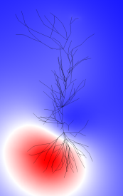
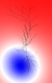
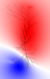
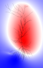
Figure 4.3: Solution of the full three-scale model framework: propagation of an extracellular action-potential into homogeneous extracellular space.

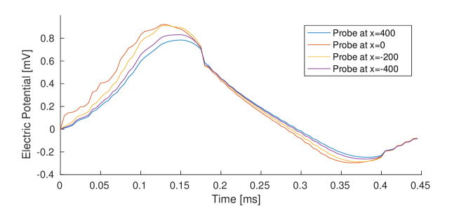
Figure 4.4: Electric potential (mV) in the four point probes placed around the neuron.

5 Conclusions

In this paper we have proposed a model framework for neuronal firing processes consisting of three layers: on the microscale, ion channel gating is modeled as a continuous-time Markov chain. On the intermediate scale, the currents produced by open channels are integrated into the current-balance equation proposed by Hodgkin and Huxley. Finally, on the macroscale, the outward current of neurons are propagated into extracellular space, simulating the emission of an extracellular potential. We have also described a numerical approach to the coupling of the different scales and indicated through computational results the feasibility of the overall approach.

To date, several exact and approximate simulation methods [16, 5, 25, 18] of stochastically gated ion channel models have been proposed. However, to our knowledge, the coupling between the microscopic gating layer and the mesoscopic layer describing the action potential initiation and propagation, has not yet been rigorously studied. In this paper, we provide the formulation of the coupling as a split-step method and moreover numerically observe the convergence of the method with respect to the size of the coupling time-step as well as the spatial discretization. We show that the distribution of interspike intervals may be significantly affected by the choice of the coupling time-step, but does not appear to depend strongly on the spatial discretization. Finally, we discuss the theory and praxis of incorporating the macroscopic scale into the model, including the spatial representation of neuronal compartments and appropriate numerical procedures for the simulation of the local field potential (LFP) propagation.

While it has often been taken for granted that ion channel gating occurs deterministically, accumulating research evidence indicates that the presence of stochasticity significantly influences the neuronal behavior [32, 35, 15]. In turn, neurons respond with a high level of variability to the repeated presentation of equal stimuli. This leads to remarkable difficulties in studying the link between single cell biophysical properties and their function in larger neuronal networks, both in health and disease. Additionally, a recent study [5] has shown that stochastic ion channel gating largely differs not only between different neuronal cell types, but also locally between different parts of the neuron. Given the technical difficulties of assessing the signal channel properties of smaller neuronal compartments such as axons and dendrites, developing reliable mathematical models is essential to tackle this problem.

Several studies [32, 35, 15, 5, 33, 27] have demonstrated how incorporation of channel noise into the Hodgkin and Huxley equations could resemble multiple realistic neuronal behaviors. Although it is not the scope of this work to mimic any particular experimental problem, but rather to provide a modeling framework that could be used by a diverse group of scientists in the future, we foresee multiple interesting applications. For example, it was shown previously [24, 34, 35] that the stochastic nature of voltage-gated ion channels in the medial entorhinal cortex stellate cells are crucial for generating subthreshold oscillations in theta ($\approx 8$Hz) frequency range. These intrinsic oscillations in stellate cells were suggested to generate theta oscillations in vivo LFP [34]. It is well established that theta oscillatory activity in vivo provides a temporal window in which spatial and declarative memories are formed [19]. Thus, our framework could be used to test the link between the stochastic nature of single channels in specific cell types and their effect at both the cellular and the network level.

Availability and reproducibility

The computational results can be reproduced within the upcoming release 1.4 of the URDME open-source simulation framework, available for download at www.urdme.org.

References

- Anastassiou et al. [2011] C. A. Anastassiou, R. Perin, H. Markram, and C. Koch. Ephaptic coupling of cortical neurons. Nature Neuroscience, 14(2):217–223, 2011.
- Bédard et al. [2004] C. Bédard, H. Kröger, and A. Destexhe. Modeling extracellular field potentials and the frequency-filtering properties of extracellular space. Biophysical Journal, 86(3):1829–1842, 2004.
- Bhalla et al. [1992] U. S. Bhalla, D. H. Bilitch, and J. M. Bower. Rallpacks: a set of benchmarks for neuronal simulators. Trends in Neurosciences, 15(11):453 – 458, 1992.
- Buzsáki et al. [2012] G. Buzsáki, C. A. Anastassiou, and C. Koch. The origin of extracellular fields and currents — EEG, ECoG, LFP and spikes. Nature Reviews Neuroscience, 13(6):407–420, 2012.
- Cannon et al. [2010] R. C. Cannon, C. O’Donnell, and M. F. Nolan. Stochastic Ion Channel Gating in Dendritic Neurons: Morphology Dependence and Probabilistic Synaptic Activation of Dendritic Spikes. PLoS Computational Biology, 6(8), 2010.
- Chevallier and Engblom [2017] A. Chevallier and S. Engblom. Pathwise error bounds in multiscale variable splitting methods for spatial stochastic kinetics, 2017. Accepted for publication in SIAM J. Numer. Anal. Available at https://arxiv.org/abs/1607.00805.
- Com [2012] AC/DC Module User’s Guide. Comsol, 2012. Version 4.3.
- Crank and Nicolson [1947] J. Crank and P. Nicolson. A practical method for numerical evaluation of solutions of partial differential equations of the heat-conduction type. Advances in Computational Mathematics, 6(1):207–226, 1947.
- Cuntz et al. [2010] H. Cuntz, F. Forstner, A. Borst, and M. Häusser. One Rule to Grow Them All: A General Theory of Neuronal Branching and Its Practical Application. PLoS Computational Biology, 6(8), 2010.
- Dorval and White [2005] A. D. Dorval and J. A. White. Channel noise is essential for perithreshold oscillations in entorhinal stellate neurons. The Journal of Neuroscience: The Official Journal of the Society for Neuroscience, 25(43):10025–10028, 2005.
- Einevoll et al. [2010] G. T. Einevoll, D. K. Wójcik, and A. Destexhe. Modeling extracellular potentials. Journal of Computational Neuroscience, 29(3):367–369, 2010.
- Einevoll et al. [2013] G. T. Einevoll, C. Kayser, N. K. Logothetis, and S. Panzeri. Modelling and analysis of local field potentials for studying the function of cortical circuits. Nature Reviews Neuroscience, 14(11):770–785, 2013.
- Engblom [2015] S. Engblom. Strong convergence for split-step methods in stochastic jump kinetics. SIAM Journal of Numerical Analysis, 53(6):2655–2676, 2015.
- Ethier and Kurtz [1986] S. N. Ethier and T. G. Kurtz. Markov Processes: Characterization and Convergence. Wiley series in Probability and Mathematical Statistics. John Wiley & Sons, New York, 1986.
- Faisal et al. [2008] A. A. Faisal, L. P. J. Selen, and D. M. Wolpert. Noise in the nervous system. Nature Reviews Neuroscience, 9(4):292–303, 2008.
- Fox [1997] R. F. Fox. Stochastic versions of the Hodgkin-Huxley equations. Biophysical Journal, 72(5):2068–2074, May 1997.
- Gillespie [1977] D. T. Gillespie. Exact stochastic simulation of coupled chemical reactions. Journal of Physical Chemistry, 81(25):2340–2361, 1977.
- Goldwyn et al. [2011] J. H. Goldwyn, N. S. Imennov, M. Famulare, and E. Shea-Brown. Stochastic differential equation models for ion channel noise in Hodgkin-Huxley neurons. Physical Review. E, Statistical, Nonlinear, and Soft Matter Physics, 83(4 Pt 1):041908, 2011.
- Hartley et al. [2014] T. Hartley, C. Lever, N. Burgess, and J. O’Keefe. Space in the brain: how the hippocampal formation supports spatial cognition. Philosophical Transactions of the Royal Society of London. Series B, Biological Sciences, 369(1635):20120510, 2014.
- Hendrickson et al. [2011] E. B. Hendrickson, J. R. Edgerton, and D. Jaeger. The capabilities and limitations of conductance-based compartmental neuron models with reduced branched or unbranched morphologies and active dendrites. Journal of Computational Neuroscience, 30(2):301–321, 2011.
- Hille [1992] B. Hille. Ionic Channels of Excitable Membranes. Sinauer Associates, 1992.
- Hodgkin and Huxley [1952] A. L. Hodgkin and A. F. Huxley. A quantitative description of membrane current and its application to conduction and excitation in nerve. The Journal of Physiology, 117(4):500–544, 1952.
- Jin [2002] J. Jin. The Finite Element Method in Electromagnetics. John Wiley & Sons, New York, 2nd edition, 2002.
- Klink and Alonso [1993] R. Klink and A. Alonso. Ionic mechanisms for the subthreshold oscillations and differential electroresponsiveness of medial entorhinal cortex layer II neurons. Journal of Neurophysiology, 70(1):144–157, 1993.
- Linaro et al. [2011] D. Linaro, M. Storace, and M. Giugliano. Accurate and fast simulation of channel noise in conductance-based model neurons by diffusion approximation. PLoS Computational Biology, 7(3):e1001102, 2011.
- Marasco et al. [2013] A. Marasco, A. Limongiello, and M. Migliore. Using Strahler’s analysis to reduce up to 200-fold the run time of realistic neuron models. Scientific Reports, 3:srep02934, 2013.
- Moezzi et al. [2016] B. Moezzi, N. Iannella, and M. D. McDonnell. Ion channel noise can explain firing correlation in auditory nerves. Journal of Computational Neuroscience, 41(2):193–206, 2016.
- Morse et al. [2010] T. M. Morse, N. T. Carnevale, P. G. Mutalik, M. Migliore, and G. M. Shepherd. Abnormal Excitability of Oblique Dendrites Implicated in Early Alzheimer’s: A Computational Study. Frontiers in Neural Circuits, 4, 2010.
- Purves [2012] D. Purves. Neuroscience. Sinauer Associates, 2012. 4th Edition.
- Rees et al. [2000] D. C. Rees, G. Chang, and R. H. Spencer. Crystallographic Analyses of Ion Channels: Lessons and Challenges. Journal of Biological Chemistry, 275(2):713–716, 2000.
- Riedler [2013] M. G. Riedler. Almost sure convergence of numerical approximations for piecewise deterministic Markov processes. Journal of Computational and Applied Mathematics, 239(0):50–71, 2013.
- Schneidman et al. [1998] E. Schneidman, B. Freedman, and I. Segev. Ion channel stochasticity may be critical in determining the reliability and precision of spike timing. Neural Computation, 10(7):1679–1703, 1998.
- Stiefel et al. [2013] K. M. Stiefel, B. Englitz, and T. J. Sejnowski. Origin of intrinsic irregular firing in cortical interneurons. Proceedings of the National Academy of Sciences of the United States of America, 110(19):7886–7891, 2013.
- White et al. [1998] J. A. White, R. Klink, A. Alonso, and A. R. Kay. Noise from voltage-gated ion channels may influence neuronal dynamics in the entorhinal cortex. Journal of Neurophysiology, 80(1):262–269, 1998.
- White et al. [2000] J. A. White, J. T. Rubinstein, and A. R. Kay. Channel noise in neurons. Trends in Neurosciences, 23(3):131–137, 2000.