Energetics of H₂ clusters from density functional and coupled cluster theories

Abstract

We use coupled-cluster quantum chemical methods to calculate the energetics of molecular clusters cut out of periodic molecular hydrogen structures that model observed phases of solid hydrogen. The hydrogen structures are obtained from Kohn-Sham density functional theory (DFT) calculations at pressures of 150, 250 and 350 GPa, which are within the pressure range in which phases II, III and IV are found to be stable. The calculated deviations in the DFT energies from the coupled-cluster data are reported for different functionals, and optimized functionals are generated which provide reduced errors. We give recommendations for semi-local and hybrid density functionals that are expected to accurately describe hydrogen at high pressures.

The phase diagram of solid hydrogen has been studied theoretically using a number of approaches such as density functional theory (DFT) Jones_2015 , diffusion quantum Monte Carlo (DMC) Ceperley_Alder_1980 , Foulkes_RMP_2001 , and path integral molecular dynamics (PIMD) methods PIMD_Marx_1996 , PIMD_Kitamura_2000 , PIMD_H_Chen_2013 , PIMD_H_Li_2013 . The hexagonal structure of phase I of solid hydrogen was obtained from experiment long ago Silvera_1980 , Mao_1994 . Structures for solid hydrogen at high-pressures have been proposed from the DFT-based ab initio random structure searching method silane_Pickard_2006 , structure_search_Pickard_2011 , structure_search_Needs_2016 . These structures provide models for phases III III_H_Pickard_2007 , IV DFT_H_IV_Pickard_2012 and, with less certainty, for phase II DFT_H_II_2009 of solid hydrogen which are in reasonable agreement with the available vibrational data from infra-red and Raman spectroscopy Dalladay-Simpson_2016 , Zha_experiment_phase_IV_2013 , Howie_phase_IV_H_and_D_2012 , Loubeyre_H_2002 , Zha_IR_360_GPa_2012 , Howie_Mixed_Molecular_and_Atomic_Phase_hydrogen_2012 , Eremets_Conductive_dense_hydrogen_2011 , Goncharov_vibron_H2_D2_200GPa_2011 . A hexagonal structure has recently been proposed as a model for the low-pressure range of phase III Monserrat_2016 , but it is not considered in this work. DMC has been used to benchmark DFT results for solid hydrogen at high pressures H_He_McMahon_2012 , Morales_2013 , QMC_bulk_H_Azadi_2014 , Clay_2014 , QMC_bulk_H_Drummond_2015 , although the expense of the DMC calculations means that only very limited data could be generated.

Here we construct exchange-correlation functionals that can be expected to provide an accurate description of the energetics of the structures mentioned above within DFT. Two accurate hybrid functionals are provided, denoted O₁ and O₁-D3, for use without and with dispersion corrections, respectively. We also provide accurate generalized gradient approximation (GGA) functionals (though less accurate than their hybrid counterparts), denoted O₃ and O₃-D3, for use without and with dispersion corrections, respectively. DMC energies are computed using orbitals generated with one of the functionals and compared with results from coupled cluster singles, doubles, and perturbative triples [CCSD(T)] in order to further assess the accuracy of the hydrogen functionals.

I Generation of H₂ cluster geometries

We use small molecular hydrogen clusters as reference systems to construct our DFT functionals. We extract cluster geometries from stable bulk DFT structures obtained with the PBE semi-local density functional by taking spherical cuts of each system containing up to 24 hydrogen atoms. Total energy calculations for a variety of clusters of hydrogen molecules are carried out at the level of CCSD(T) and DFT. The coupled cluster and DFT calculations are performed using the MOLPRO code molpro .

The procedure for generating cluster geometries is designed to give reasonably compact and symmetric structures and is as follows. For a bulk structure, atomic pairs closer than $0.85$ Å are classified as molecules. The distance parameter used in this classification is chosen so that all atoms are classified as a member of only one molecule. The center of mass of each H₂ molecule and the midpoint between the center of mass of pairs of molecules is then recorded.

For clusters with an even number of molecules, a sphere is centered at each midpoint and expanded until it contains the required number of hydrogen atoms, $N$. For clusters with an odd number of molecules, a sphere is placed at the center of mass of each H₂ molecule and expanded until it contains $N$ hydrogen atoms. This procedure is carried out for each midpoint/center-of-mass, and we select the point about which the magnitude of the first moment of the selected atomic positions is minimized. This process preserves much of the symmetry of the underlying bulk structure, and supplies compact clusters representing each structure.

Clusters are generated from the bulk structures of symmetries $P2_{1}c$-24, $C2/c$-24, and $Pc$-48, which model, respectively, phases II, III, and IV of hydrogen, while $Cmca$-12 and $Cmca$-4 are other low-energy structures that have been found in structure searches. (Note that in this notation the number of atoms in the primitive unit cell is given following the space group designation.) The five structures are calculated using DFT at pressures of 150, 250, and 350 GPa, which covers the experimentally relevant high-pressure regime. Clusters containing 1–12 pairs of hydrogen atoms are generated from each of these structures, providing a total of 180 clusters.

II Extrapolation and error assessment for CCSD(T) and DFT

CCSD(T) calculations are performed to provide reference energies for each cluster which accurately include many-body effects. These reference energies are then compared with DFT energies for several exchange-correlation functionals. The cc-pV$n$Z Gaussian basis sets are used basis_dunning_1992 , together with extrapolation to the complete basis set (CBS) limit. Note that $n={\rm D},{\rm T},{\rm Q},5,6,\ldots$ specifies the largest value of the angular momentum index $l$ in the basis set.

A variety of procedures are available in the literature to extrapolate CCSD(T) results to the CBS limit cbslim_feller_2013 . We employ a computationally expensive extrapolation procedure, which we refer to as “accurate extrapolation”, for small clusters containing 2–8 hydrogen atoms. These “accurate” total energies are then used to validate an empirical, but computationally cheaper, extrapolation procedure that is applied to all cluster sizes, which we refer to as “efficient extrapolation”.

The CCSD(T) energy is given by

$$E_{\rm CCSD(T)}=E_{\rm HF}+E_{\rm S}+E_{\rm D}+E_{\rm(T)}\;,$$ (1)

where $E_{\rm HF}$ is the Hartree-Fock (HF) energy, $E_{\rm S}$ is the second-order contribution to the correlation energy due to double excitations of opposite-spin electrons, $E_{\rm D}$ is the second-order contribution to the correlation energy due to double excitations of like-spin electrons, and $E_{\rm(T)}$ is the perturbative triple-excitation correlation energy. We extrapolate the CCSD(T) energies of the smaller clusters to the CBS limit using analytic forms justified by the expected asymptotic behavior of the components of the CCSD(T) energy extrap_ranasinghe_2013 ,

$$E_{\rm HF}(n) = E_{\rm HF}(\infty)+a_{0}e^{-b_{0}\sqrt{n}}\;,$$ (2)

$$E_{\rm S}(n) = E_{\rm S}(\infty)+a_{1}\left(n+c_{1}\right)^{-3}+b_{1}\left(n+c_{1}\right)^{-5}\;,$$ (3)

$$E_{\rm D}(n) = E_{\rm D}(\infty)+a_{2}\left(n+c_{2}\right)^{-5}+b_{2}\left(n+c_{2}\right)^{-7}\;,$$ (4)

$$E_{\rm(T)}(n) = E_{\rm(T)}(\infty)+a_{3}\left(n+c_{3}\right)^{-3}+b_{3}\left(n+c_{3}\right)^{-5}\,,\;\;\;\;$$ (5)

where the left-hand sides of the equations are the components of the CCSD(T) energy evaluated with the cc-pV$n$Z basis set, $\{a_{i},b_{i},c_{i}\}$ are fitting parameters describing the variation of the energy components with $n$, and $E_{\rm HF}(\infty)$, $E_{\rm S}(\infty)$, $E_{\rm D}(\infty)$, and $E_{\rm(T)}(\infty)$ are the extrapolated energy components, which are treated as fitting parameters. Values of the left-hand sides are collected from CCSD(T) calculations using basis sets with $n={\rm T},{\rm Q},5,6$, and a least-squares fit for each component then provides the estimated CBS total energy.

This extrapolation is expected to be accurate due to the analytically justified forms for each component of the total energy, and because including higher order terms in the correlation energy expressions ensures that the variation of energy with basis set size is accurately described for the smaller basis sets. The absolute deviation $|E_{\rm CCSD(T)}(6)-E_{\rm CCSD(T)}(\infty)|$ is expected to severely overestimate the error in this extrapolation process, hence the mean and maximum absolute deviations of $4.6$ and $5.4$ meV/[H₂] for clusters of 2–8 hydrogen atoms reliably validate this finite basis correction.

Next, we use these “accurate” total energies to validate a computationally cheaper extrapolation method for application to the full set of clusters. The variation of the total energy with basis set is dominated by the $E_{\rm S}(n)$ term, hence we take the lowest-order part of $E_{\rm S}(n)$ to construct our estimated CBS limit, $E_{\rm est}$. We also estimate an extrapolation error interval by using similar forms with different powers to define upper and lower limits, $E_{\rm u}$ and $E_{\rm l}$, with values of the powers chosen so that the estimated range includes the “accurate” estimates for the small clusters of 2–8 hydrogen atoms.

The resulting “efficient extrapolation” procedure takes the form

$$E_{\rm u}(n) = E_{\rm u}(\infty)+a_{\rm u}\left(n+n_{0}\right)^{-\frac{5}{2}}\;,$$ (6)

$$E_{\rm est}(n) = E_{\rm est}(\infty)+a_{\rm est}\left(n+n_{0}\right)^{-3}\;,$$ (7)

$$E_{\rm l}(n) = E_{\rm l}(\infty)+a_{\rm l}\left(n+n_{0}\right)^{-\frac{7}{2}}\;,$$ (8)

where $E_{\rm u}(\infty)$, $E_{\rm est}(\infty)$, $E_{\rm l}(\infty)$, $a_{\rm u}$, $a_{\rm est}$ and $a_{\rm l}$ are fitting parameters, and $n_{0}$ is fixed to the average value of $c_{1}$ in Eq. (3), with $n_{0}=-0.838$. The two free parameters in each equation are obtained for each cluster from CCSD(T) energies calculated using the two largest available basis sets, resulting in an estimated CBS limit given by $E_{\rm est}(\infty)$ and an estimated error of $[E_{\rm u}(\infty)-E_{\rm l}(\infty)]/2$.

For the subset of small clusters with $N=2$–8 the “efficient” procedure provides total energies that agree with the “accurate” values to within the estimated error ranges. The mean absolute errors for small clusters using “efficient” (TQ), (Q5) and (56) extrapolation are $6.1$, $2.6$, and $1.0$ meV/[H₂], respectively, where we use the notation $(n_{1}n_{2})$ to denote “efficient extrapolation” from results with the cc-pV$n_{1}$Z and cc-pV$n_{2}$Z basis sets. The “efficiently” estimated energies and confidence intervals for each small cluster geometry are shown in Fig. 1 as a deviation from the “accurate” estimates.

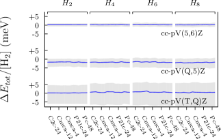
Figure 1: “Efficient” estimates of CCSD(T) total energies, and the associated confidence intervals, plotted as the deviation from “accurate” total energies. Estimates are given for three different pairs of basis sets, and for geometries containing 8 hydrogen atoms or fewer. The gray shaded regions show the error ranges associated with the “efficient extrapolation” procedure.

The convergence of the DFT total energies with basis set is exponential due to the correlation being contained in the exchange-correlation functional rather than the wave function itself. Consequently, extrapolation using only Eq. (2) provides accurate estimates of the CBS limit (replacing $E_{\rm HF}$ with the DFT energy). In a similar manner to the CCSD(T) calculations, we begin with an “accurate” estimate of the finite basis correction for the geometries with $N=2$–12. The CBS total energy is provided by a least-squares fit of Eq. (2) to results obtained with the $n={\rm D},{\rm T},{\rm Q},5$ basis sets, and with all parameters free.

The absolute deviation $|E_{\rm KS}(5)-E_{\rm KS}(\infty)|$ is expected to severely overestimate the extrapolation error, hence mean and maximum absolute deviations of $1.4$ and $4.4$ meV/[H₂] for clusters of 2–12 hydrogen atoms reliably validate this finite-basis correction. Note that these mean and maximum deviations are taken over all of the exchange-correlation functionals considered as well as the range of cluster sizes.

Then, we construct an “efficient” estimate of the CBS limit by two-point extrapolation using Eq. (2) with $b_{0}$ fixed to its average value for the “accurate” extrapolations, where $b_{0}=6.707$. Upper and lower limits are provided by extrapolation using the maximum and minimum $b_{0}$ values ($b_{0}=8.247$ and $4.257$). This provides estimated values and error ranges in a similar manner to the CCSD(T) approach, with mean errors of $19.7$, $2.6$, and $0.9$ meV/[H₂] for (DT), (TQ), and (Q5) extrapolations, respectively.

Further basis set errors are expected to remain after extrapolation due to superposition and the finite range of the cc-pV$n$Z basis sets. These are found to be negligible (see Supplementary Material supplementary ).

III Optimum exchange-correlation functionals

Eight new exchange-correlation functionals are constructed by taking the components of the B3LYP functional B3LYP_Kim_1994 and determining their coefficients by minimizing the average difference between the CCSD(T) and DFT energies using an iterative approach. At iteration $i$, the total DFT energy provided by these B3LYP-like functionals is of the form

$$E_{\rm KS}[\rho_{i}] = T[\rho_{i}]+V[\rho_{i}]+\alpha_{0}^{(i)}E_{\rm x}^{\rm HF}[\rho_{i}]+$$

$$\alpha_{1}^{(i)}E_{\rm x}^{\rm B88}[\rho_{i}]+\alpha_{2}^{(i)}E_{\rm x}^{\rm LDA}[\rho_{i}]+$$

$$\alpha_{3}^{(i)}E_{\rm c}^{\rm LYP}[\rho_{i}]+\alpha_{4}^{(i)}E_{\rm c}^{\rm LDA}[\rho_{i}]+E_{\rm D3}\;,$$

where $\rho_{i}$ is the electronic density, $\alpha_{j}^{(i)}$ are linear parameters, $E_{\rm x}^{\rm HF}$ is the exact Hartree-Fock exchange energy, $E_{\rm x}^{\rm B88}$ and $E_{\rm c}^{\rm LYP}$ are the BLYP-parameterized exchange and correlation functionals, and $E_{\rm x}^{\rm LDA}$ and $E_{\rm c}^{\rm LDA}$ are the parameterized local density approximation (LDA) exchange and correlation functionals. The final term is a dispersion correction, $E_{\rm D3}$.

The iterative method works as follows. Parameter values at the start of iteration $i$, $\{\alpha_{j}^{(i)}\}$, provide a DFT density $\rho_{i}$. We then define the penalty function,

$$P_{i}\left(\{\alpha_{j}^{(i)}\}\right)=\sum_{k}\left[\frac{E^{k}_{\rm KS}[\rho_{i}]\left(\{\alpha_{j}^{(i)}\}\right)-E^{k}_{\rm CCSD(T)}}{N_{k}}\right]^{2},$$ (10)

where index $k$ runs over all 180 clusters considered, and $E^{k}_{\rm CCSD(T)}$ is the best available “efficiently extrapolated” CCSD(T) energy for the $k$th cluster. “Efficient” (DT) extrapolation of DFT energies is used to limit the computational cost.

The penalty function is then minimized with respect to $\{\alpha_{j}^{(i)}\}$ with the density fixed to $\rho_{i}$. Due to linearity this is easily achieved using matrix diagonalization, and provides the optimum fixed-density parameters for $\rho_{i}$, $\{\alpha_{j}^{(i+1)}\}$. This process is then repeated until the variation in parameter values and total energies is sufficiently small.

Four of the eight optimum functionals generated (O₁, O₂, O₃, and O₄) do not include dispersion corrections ($E_{\rm D3}=0$), while the rest (O₁-D3, O₂-D3, O₃-D3, and O₄-D3) include that of Grimme et al. disp_Grimme_2010 . Dispersion corrections optimized for each functional are used when available, and when unavailable BLYP corrections are used for GGA functionals (LDA, PW91, O₃-D3 and O₄-D3) and B3LYP corrections for hybrid functionals (SOGGA11-X, B3H, M08-SO, O₁-D3 and O₂-D3).

We generate four hybrid functionals that include exact exchange [O₁(-D3) and O₂(-D3)] and four GGA functionals that exclude exact exchange [O₃(-D3) and O₄(-D3)]. Four of the functionals are constrained to obey the homogeneous electron gas (HEG) limit [O₂(-D3) and O₄(-D3)], and the remaining four [O₁(-D3) and O₃(-D3)] are not required to obey the HEG limit.

Convergence is rapid for all eight functionals, with changes in the total energy falling to less than $10^{-3}$ meV/[H₂] after four iterations. Optimum parameters and constraints are reported in Table 1.

The error in the total energy estimates used for optimization is small. The CBS total energies obtained with (DT) extrapolation incur a maximum estimated error of 36 meV/[H₂]. This is an overestimate; the maximum difference between energies obtained using (DT) extrapolation and those obtained using larger basis sets (see the next section) is 8 and 13 meV/[H₂] for the optimum functionals that satisfy or do not satisfy the HEG limit, respectively.

	Exchange						Correlation
Functional	$\alpha_{0}$		$\alpha_{1}$		$\alpha_{2}$		$\alpha_{3}$		$\alpha_{4}$
O1	$0$.	$60354910205605$	$0$.	$14589659222789$	($1-\alpha_{0}-\alpha_{1}$)		$0$.	$54819918079350$	($1-\alpha_{3}$)
O2	$0$.	$76679614121531$	$-0$.	$84277505048128$	$1$.	$05244207765216$	$-1$.	$85005839047496$	$2$.	$33023683529908$
O3	($0$)		$0$.	$79872851641853$	($1-\alpha_{0}-\alpha_{1}$)		$0$.	$61544187700225$	($1-\alpha_{3}$)
O4	($0$)		$1$.	$29167530141040$	$-0$.	$25869459399816$	$2$.	$03890740504165$	$-0$.	$86103233660732$
O1-D3	$0$.	$49200298266553$	$0$.	$34311594882336$	($1-\alpha_{0}-\alpha_{1}$)		$0$.	$67727856886346$	($1-\alpha_{3}$)
O2-D3	$0$.	$61183767165887$	$-0$.	$39108315837275$	$0$.	$76213024756349$	$-1$.	$10597328426091$	$1$.	$72092162085949$
O3-D3	($0$)		$0$.	$90916334640647$	($1-\alpha_{0}-\alpha_{1}$)		$0$.	$78790801474948$	($1-\alpha_{3}$)
O4-D3	($0$)		$1$.	$38553958317866$	$-0$.	$35884244275049$	$2$.	$16733823510143$	$-0$.	$96208190626903$
B3LYP	$0$.	$20000000000000$	$0$.	$72000000000000$	$0$.	$08000000000000$	$0$.	$81000000000000$	$0$.	$19000000000000$

Table 1: Parameters that define the optimized functionals used. Parameters for the standard B3LYP functional are also shown, for comparison.

IV Results

We quantify the performance of exchange-correlation functionals by their ability to reproduce the CCSD(T) total energies for the H₂ clusters. In addition to our optimum functionals, we test 11 standard functionals readily available in the literature: one LDA, four GGA, and six hybrid functionals that combine exact exchange and semi-local exchange-correlation functionals. We test the functionals with and without dispersion corrections, providing a total of 30 distinct DFT Hamiltonians (see Table 2).

Functional	Type
LDA	Local
PBE PBE_Perdew_1996	GGA
BLYP BLYP_Becke_1988	GGA
revPBE PBEREV_Zhang_1998	GGA
PW91 PW91_Perdew_1992	GGA
O3(-D3)	GGA
O4(-D3)	GGA
PBE0 PBE0_Adamo_1999	Hybrid
SOGGA11-X SOGGA11_Peverati_2011	Hybrid
B3H B3H_chermette_1997	Hybrid
B97 B97_Grimme_2006	Hybrid
B3LYP B3LYP_Kim_1994	Hybrid
M08-SO M08set_Zhao_2008	Hybrid (meta)
O1(-D3)	Hybrid
O2(-D3)	Hybrid

Table 2: Functionals used and their types.

Calculations are performed using cc-pV$n$Z basis sets with different $n$ for different clusters, and for CCSD(T) and DFT. “Efficient” extrapolation to the CBS limit, together with the estimation of the extrapolation error, is performed as described previously.

In the CCSD(T) calculations we use (56), (Q5), and (TQ) extrapolations for clusters of $N=2$–$8$, $10$–$12$, and $14$–$24$ atoms, respectively, obtaining mean basis set errors in the extrapolated total energies of $1.0$, $2.9$, and $7.3$ meV/[H₂]. In the DFT calculations we use (Q5) and (TQ) extrapolations for clusters of $N=2$–$12$ and $14$–$24$ atoms, respectively, obtaining mean errors in the DFT energies of $0.9$ and $2.6$ meV/[H₂]. (For DFT mean values of errors are evaluated over all functionals, as well as geometries.) This energy resolution is sufficient to assess the accuracy of exchange-correlation functionals.

Each error is quantified as the deviation of the DFT energy from the CCSD(T) energy, $\Delta=E_{\rm KS}-E_{\rm CCSD(T)}$. Errors for each functional are summarized as both the mean and maximum absolute difference for all clusters in Fig. 2 for functionals with and without dispersion corrections.

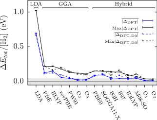
Figure 2: Maximum and mean absolute differences between DFT and CCSD(T) total energies for a variety of exchange-correlation functionals, both including ($\Delta_{\rm DFT{\mathchar 45\relax}D3}$) and excluding ($\Delta_{\rm DFT}$) dispersion corrections. The maximum and mean is taken over the 180 geometries considered, and basis set errors are almost imperceptible. Differences in the gray shaded region denote an accuracy of better than the chemical accuracy tolerance of $1$ kcal mol${}^{-1}=43$ meV/[H₂].

As expected, LDA energies are significantly worse than those from all GGA and hybrid functionals, resulting in a peak error of ${\sim}1$ eV/[H₂] for H₂ that slowly falls with increasing cluster size. Most of the LDA error may be identified with an imperfect correction to the self-interaction (SI) included in the Coulomb potential for DFT as this results in an error of $1.2$ eV/[H₂] for an isolated hydrogen atom. The improved accuracy of the non-LDA functionals is, in part, due to their improved treatment of SI.

The general trend in Fig. 2 is for hybrid functionals to be more accurate than GGA functionals, with the optimized functionals providing the smallest errors for both types. However, there is considerable overlap between errors for the two functional types. Of the hybrid functionals, only B3LYP and the optimized functionals are more accurate than the optimized GGA functionals, whether or not dispersion is present.

Given the fitting procedure and the extra variational freedom allowed by relaxing the HEG limit, we would expect O₂-D3 and O₄-D3 functionals to reproduce the CCSD(T) results to the highest accuracy. This is the case, with the lowest peak error for the hybrid functionals of 32(3) meV/[H₂] provided by O₂-D3, and the lowest peak error for the GGA functionals of 92(3) meV/[H₂] provided by O₄-D3. However, the O₁-D3 and O₃-D3 functionals, which are constrained to reproduce the HEG limit, perform only marginally worse, with peak errors of 35(3) meV/[H₂] and 104(3) meV/[H₂], respectively.

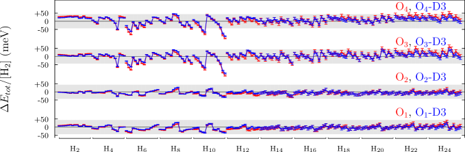
Figure 3: Deviation of DFT total energies from the CCSD(T) total energies. Results with (blue) and without (red) dispersion are shown. Values and errors bars are obtained using the “efficient” estimates described in the text, and differences in the gray shaded regions denote an accuracy of better than the chemical accuracy tolerance of $1$ kcal mol${}^{-1}=43$ meV/[H₂].

Dispersion provides no consistent improvement to the performance of the functionals considered. The introduction of dispersion increases the peak error for 5 of the 15 functionals, leaves it unchanged for another 5, and decreases it for the other 5 functionals. Unsurprisingly, functionals optimized with dispersion give marginally better results when applied with dispersion than without, and vice versa. This effect is not shown in the figures.

In order to gain further insight into the performance of the functionals, in Fig. 3 we plot the deviation of the DFT energies using the O_n(-D3) functionals from the CCSD(T) energies for each of the 180 clusters. Data generated with and without dispersion exhibit the same structure, confirming that dispersion has a small effect on the results. Overall, the hybrid functionals reproduce the CCSD(T) for all clusters to within chemical accuracy, typically associated with a tolerance of 1 kcal mol${}^{-1}=43$ meV/[H₂].

For the optimum GGA functionals, O₃(-D3) and O₄(-D3), the deviations from CCSD(T) are larger in magnitude, occasionally exceeding the chemical accuracy tolerance, and display more structure than those for the hybrid functionals. Figure 3 shows segments of steep (approximately) linear variation with the pressure of the underlying bulk structure, where each segment is associated with a different symmetry and cluster size. This dependence is barely apparent for the hybrid functionals.

The inaccuracy of the functionals considered is most apparent for cluster with 4–10 hydrogen atoms, and particularly for the H₁₀ clusters. This characteristic feature is identifiable for all of the GGA functionals considered, and for most of the hybrid functionals [it is not apparent for the B3H, M08-SO, O₁(-D3), and O₂(-D3) functionals].

For a number of the functionals [though not the O_n(-D3)] there is an underlying linear variation of error with cluster size. This observation, together with the known inadequate description of SI by DFT, suggests that the SI error should be included in our assessment of the accuracy of the functionals.

We estimate the SI error as the difference between the total DFT energy of an isolated hydrogen atom evaluated with each functional (using an $n=6$ finite basis set that results in a negligible basis set error) and the exact analytic energy.

Figure 4 shows the resulting SI error for each functional (dispersion is zero for an isolated atom, so there are only 19 distinct total energies to consider). The greatest SI error arises for the LDA functional. For the optimum functionals the SI error is consistently decreased by including Hartree-Fock exchange and not enforcing the HEG limit. Of all the functionals considered the SI error is smallest for the O₂ and O₂-D3 hybrid functionals, taking values of $13$ and $3$ meV/[H₂], respectively.

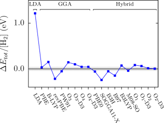
Figure 4: Self-interaction errors for an isolated hydrogen atom for the 19 functionals considered in the text, and using the exact density. Points within the gray shaded region denote a self-interaction error smaller than the chemical accuracy tolerance of 1 kcal mol${}^{-1}=43$ meV/[H₂].

Since we are seeking an accurate functional for systems very unlike the HEG, relaxing the requirement that the HEG limit is conserved in the functionals is justified. However, it is reasonable to expect that a physically realistic functional will not radically misrepresent the HEG. Whether this is so may be assessed by summing the exchange and correlation coefficients in Table 1. For all of the optimized functionals the HEG exchange is well preserved, with total HEG exchange deviating from the true value by less than 4%. The HEG correlation is significantly less accurate when the HEG limit is not enforced, deviating from the true value by more than 17% for the GGA functionals, and more than 38% for the hybrid functionals.

The proposed functionals can be used to generate single-particle orbitals for quantum Monte Carlo calculations Foulkes_RMP_2001 , which is particularly useful for studies of crystalline hydrogen structures, such as those of Refs. QMC_bulk_H_Drummond_2015, and QMC_bulk_H_Azadi_2014, , which require more accuracy than afforded by DFT and much larger systems sizes than are accessible with CCSD(T). In order to assess the accuracy of the functionals in this context we perform diffusion Monte Carlo (DMC) calculations using the casino code CASINO_review for the H₆, H₁₂, and H₂₄ clusters using single-particle orbitals generated with the O₃ GGA functional. The orbitals are cusp-corrected Ma_cusps_2005 to prevent divergences of the local energy at electron-nucleus coalescence points, and used in a Slater-Jastrow Drummond_jastrow_2005 , LopezRios_jastrow_2011 trial wave function, whose parameters are optimized using linear least-squares energy minimization Umrigar_emin_2007 , Toulouse_emin_2007 at the variational Monte Carlo level. The DMC energies are obtained using the recent modifications of Zen et al. Zen_timestep_2016 , and extrapolated to zero timestep Lee_strategies_2011 and infinite population size; additional details are given in the Supplementary Material supplementary .

The DMC energies, shown in Fig. 5, are higher than the CCSD(T) energies for all 45 clusters. Each of the successive S, D, and (T) contributions to the CCSD(T) energy is about an order of magnitude smaller than the previous one, which is expected in well-converged calculations, hence the missing correlation energy in our CCSD(T) results may reasonably be identified with the basis set error. Figure 5 also shows close agreement between DMC and CCSD energies, strongly suggesting that the small correlation energy absent from our DMC results can be identified with the triple excitations included in CCSD(T).

The energy differences CCSD(T) and DMC are smaller than $1$ kcal mol^-1, indicating that the single-particle orbitals generated with the O₃ functional are an excellent choice for performing accurate DMC calculations. The pressure dependence of the DMC energies can be attributed to the loss of accuracy of the DMC method at higher pressures.

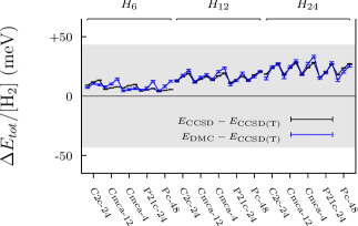
Figure 5: DMC and CCSD energies relative to CCSD(T) for the H₆, H₁₂, and H₂₄ clusters using single-particle orbitals obtained with the O₃ GGA functional. The error bars represent the statistical uncertainty in the DMC data, and the estimated basis-set extrapolation error in the CCSD data. All energy differences are smaller than the chemical accuracy tolerance of $1$ kcal mol${}^{-1}=43$ meV/[H₂] indicated by the gray shaded region.

In summary, the optimized functionals provide the best description of the total energies for the 180 clusters considered, with optimized hybrid functionals being the most accurate. Relaxing the natural requirement that the functionals reproduce the HEG limit provides an insignificant or small increase in the accuracy of the functionals, at the cost of an inaccurate description of the HEG correlation. Dispersion corrections are small for the optimized functionals.

These points suggest that the functionals of choice for hydrogen systems is the hybrid functional O₁(-D3), with O₃(-D3) a second choice if a GGA is preferred. The two different forms are available for application with or without dispersion corrections. With dispersion excluded, these provide an accuracy of better than 118(3) and 36(1) meV/[H₂] for GGA and hybrid functionals, respectively. With dispersion included, these provide an accuracy of better than 104(3) and 35(3) meV/[H₂] for GGA and hybrid functionals, respectively.

There are several obvious options to improve the accuracy of optimized functionals for hydrogen clusters. The most evident improvement would be to reduce the remnant of basis set error that arises from the extrapolation to the CBS limit used during functional optimization. This would be computationally expensive, and is probably not significant given that the structure shown in Fig. 4 is accurately reproduced by (DT), (TQ), or (Q5) extrapolation, so is not due to basis set error. Another simple option would be to dynamically allocate weights in the optimization process in order to equalize the distribution of errors between clusters. This would reduce the peak error at the cost of introducing a larger error for clusters containing 12 hydrogen atoms or more.

Perhaps the most promising option for improving the functionals would be to add more variational freedom to the optimized functional. The simplest approach would be to include other parameterizations of semi-local functionals, including meta terms, as this would preserve the linearity of the optimization we rely on within the iterative optimization process. A more general approach would be to directly optimize the enhancement factors present within the functional forms, introducing non-linearity into each optimization iteration. Similarly, the screening parameters present in the dispersion correction may also be optimized, but it seems likely that this will only provide a marginal improvement in the accuracy of the energies.

- [1] R. O. Jones, Rev. Mod. Phys. 87, 897 (2015).
- [2] D. M. Ceperley and B. J. Alder, Phys. Rev. Lett. 45, 566 (1980).
- [3] W. M. C. Foulkes, L. Mitas, R. J. Needs, and G. Rajagopal, Rev. Mod. Phys. 73, 33 (2001).
- [4] D. Marx and M. Parrinello, J. Chem. Phys. 104, 4077 (1996).
- [5] H. Kitamura, S. Tsuneyuki, T. Ogitsu, and T. Miyake, Nature 404, 259 (2000).
- [6] J. Chen, X.-Z. Li, Q. Zhang, M. I. J. Probert, C. J. Pickard, R. J. Needs, A. Michaelides, and E. Wang, Nat. Commun. 4, 2064 (2013).
- [7] X.-Z. Li, B. Walker, M. I. J. Probert, C. J. Pickard, R. J. Needs, and A. Michaelides, J. Phys.: Condens. Matter 23, 085402 (2013).
- [8] I. F. Silvera, Rev. Mod. Phys. 52, 393 (1980).
- [9] H.-K. Mao and R. J. Hemley, Rev. Mod. Phys. 66, 671 (1994).
- [10] C. J. Pickard and R. J. Needs, Phys. Rev. Lett. 97, 045504 (2006).
- [11] C. J. Pickard and R. J. Needs, J. Phys.: Condens. Matter 23, 053201 (2011).
- [12] R. J. Needs and C. J. Pickard, APL Materials 4, 053210 (2016).
- [13] C. J. Pickard and R. J. Needs, Nature Physics 3, 473 (2007).
- [14] C. J. Pickard, M. Martinez-Canales, and R. J. Needs, Phys. Rev. B 85, 214114 (2012); Erratum Phys. Rev. B 86, 059902(E) (2012).
- [15] C. J. Pickard and R. J. Needs, Phys. Status Solidi B 246, 536 (2009).
- [16] P. Dalladay-Simpson, R. T. Howie, and E. Gregoryanz, Nature 529, 63 (2016).
- [17] C.-S. Zha, Z. Liu, M. Ahart, R. Boehler, and R. J. Hemley, Phys. Rev. Lett. 110, 217402 (2013).
- [18] R. T. Howie, T. Scheler, C. L. Guillaume, and E. Gregoryanz, Phys. Rev. B 86, 214104 (2012).
- [19] P. Loubeyre, F. Occelli, and R. LeToullec, Nature 416, 613 (2002).
- [20] C.-S. Zha, Z. Liu, and R. J. Hemley, Phys. Rev. Lett. 108, 146402 (2012).
- [21] R. T. Howie, C. L. Guillaume, T. Scheler, A. F. Goncharov, and E. Gregoryanz, Phys. Rev. Lett. 108, 125501 (2012).
- [22] M. Eremets and I. Troyan, Nat. Mater. 10, 927 (2011).
- [23] A. F. Goncharov, R. J. Hemley, and H.-K. Mao, J. Chem. Phys. 134, 174501 (2011).
- [24] B. Monserrat, R. J. Needs, E. Gregoryanz, and C. J. Pickard, Phys. Rev. B 94, 134101 (2016).
- [25] J. M. McMahon, M. A. Morales, C. Pierleoni, and D. M. Ceperley, Rev. Mod. Phys. 84, 1607 (2012).
- [26] M. A. Morales, J. M. McMahon, C. Pierleoni, and D. M. Ceperley, Phys. Rev. B 87, 184107 (2013).
- [27] S. Azadi, B. Monserrat, W. M. C. Foulkes, and R. J. Needs, Phys. Rev. Lett. 112, 165501 (2014).
- [28] R. C. Clay, J. Mcminis, J. M. McMahon, C. Pierleoni, D. M. Ceperley, and M. A. Morales, Phys. Rev. B 89, 184106 (2014).
- [29] N. D. Drummond, B. Monserrat, J. H. Lloyd-Williams, C. J. Pickard, P. López Ríos, and R. J. Needs, Nat. Commun. 6, 7794 (2015).
- [30] H.-J. Werner, P. J. Knowles, R. Lindh, F. R. Manby, M. Schütz et al., molpro version 2012.1, a package of ab initio programs, http://www.molpro.net.
- [31] T. H. Dunning Jr., J. Chem. Phys. 90, 1007 (1989); R. K. Kendall, T. H. Dunning, and R. J. Harrison, J. Chem. Phys. 96, 6796 (1992).
- [32] D. Feller, J. Chem. Phys. 138, 074103 (2013).
- [33] D. S. Ranasinghe and G. A. Petersson, J. Chem. Phys. 138, 144104 (2013).
- [34] See Supplementary Material at [URL] for additional information, including a discussion of Gaussian basis-set errors, details of the DMC calculations, and full geometries of the 15 crystalline systems considered.
- [35] K. Kim and K. D. Jordan, J. Phys. Chem. 98, 10089 (1994); P. J. Stephens, F. J. Devlin, C. F. Chabalowski, and M. J. Frisch, J. Phys. Chem. 98, 11623 (1994).
- [36] S. Grimme, J. Antony, S. Ehrlich, and H. Krieg, J. Chem. Phys. 132, 154104 (2010).
- [37] J. P. Perdew, K. Burke, and M. Ernzerhof, Phys. Rev. Lett. 77, 3865 (1996); Phys. Rev. Lett. 78, 1396 (1997).
- [38] C. Lee, W. Yang, and R. G. Parr, Phys. Rev. B 37, 785 (1988); A. D. Becke, Phys. Rev. A 38, 3098 (1988).
- [39] Y. Zhang and W. Yang, Phys. Rev. Lett. 80, 890 (1998).
- [40] J. P. Perdew, J. A. Chevary, S. H. Vosko, K. A. Jackson, M. R. Pederson, D. J. Singh, and C. Fiolhais, Phys. Rev. B 46, 6671 (1992).
- [41] C. Adamo and V. Barone, J. Chem. Phys. 110, 6158 (1999).
- [42] R. Peverati, Y. Zhao, and D. G. Truhlar, J. Phys. Chem. Lett. 2, 1991 (2011); R. Peverati and D. G. Truhlar, J. Chem. Phys. 135, 191102 (2011).
- [43] H. Chermette, H. Razafinjanahary, and L. Carrion, J. Chem. Phys. 107, 10643 (1997).
- [44] S. Grimme, J. Comp. Chem. 27, 1787 (2006); S. Grimme, S. Ehrlich, and L. Goerigk, J. Comp. Chem. 32, 1456 (2011).
- [45] Y. Zhao and D. G. Truhlar, J. Chem. Theory Comput. 4, 1849 (2008).
- [46] R. J. Needs, M. D. Towler, N. D. Drummond, and P. López Ríos, J. Phys.: Condens. Matter 22, 023201 (2010).
- [47] A. Ma, M. D. Towler, N. D. Drummond, and R. J. Needs, J. Chem. Phys. 122, 224322 (2005).
- [48] N. D. Drummond, M. D. Towler, and R. J. Needs, Phys. Rev. B 70, 235119 (2004).
- [49] P. López Ríos, P. Seth, N. D. Drummond, and R. J. Needs, Phys. Rev. E 86, 036703 (2012).
- [50] C. J. Umrigar, J. Toulouse, C. Filippi, S. Sorella and R. G. Hennig, Phys. Rev. Lett. 98, 110201 (2007).
- [51] J. Toulouse and C. J. Umrigar, J. Chem. Phys. 126, 084102 (2007).
- [52] A. Zen, S. Sorella, M. J. Gillan, A. Michaelides, and D. Alfè, Phys. Rev. B 93, 241118(R) (2016).
- [53] R. M. Lee, G. J. Conduit, N. Nemec, P. López Ríos, and N. D. Drummond, Phys. Rev. E 83, 066706 (2011).