The Galaxy End Sequence

Abstract

A common assumption is that galaxies fall in two distinct regions on a plot of specific star-formation rate (SSFR) versus galaxy stellar mass: a star-forming Galaxy Main Sequence (GMS) and a separate region of ‘passive’ or ‘red and dead galaxies’. Starting from a volume-limited sample of nearby galaxies designed to contain most of the stellar mass in this volume, and thus being a fair representation of the Universe at the end of $\simeq$12 billion years of galaxy evolution, we investigate the distribution of galaxies in this diagram today. We show that galaxies follow a strongly curved extended GMS with a steep negative slope at high galaxy stellar masses. There is a gradual change in the morphologies of the galaxies along this distribution, but there is no clear break between early-type and late-type galaxies. Examining the other evidence that there are two distinct populations, we argue that the ‘red sequence’ is the result of the colours of galaxies changing very little below a critical value of the SSFR, rather than implying a distinct population of galaxies, and that Herschel observations, which show at least half of early-type galaxies contain a cool interstellar medium, also imply continuity between early-type and late-type galaxies. This picture of a unitary population of galaxies requires more gradual evolutionary processes than the rapid quenching processes needed to to explain two distinct populations. We challenge theorists to reproduce the properties of this ‘Galaxy End Sequence’.

1 Introduction

During the last decade, astronomers have developed a simple phenomenological model of galaxy evolution. In this model, star-forming galaxies lie on the ‘galaxy main sequence’ (henceforth GMS), a distinct region in a plot of star-formation rate versus galaxy stellar mass (e.g. Noeske et al. 2007; Daddi et al. 2007; Elbaz et al. 2007; Rodighiero et al. 2011; Whitaker et al. 2012; Lee et al. 2015). Over cosmic time, the GMS gradually moves downwards in star-formation rate, decreasing by a factor of $\simeq$20 from a redshift of 2 to the current epoch (Daddi et al. 2007), with the cause of the evolution in the GMS being the gradual decrease in the gas content of galaxies (Tacconi et al. 2010; Dunne et al. 2011; Genzel et al. 2015; Scoville et al. 2016). An individual galaxy evolves along the GMS until some process quenches the star-formation, and the galaxy then moves rapidly (in cosmic terms) across the diagram to the region occupied by ‘red and dead’ or ‘passive’ galaxies.

Much of the physics behind this phenomenological model is unknown. The GMS is not as narrow as the stellar main sequence, with a dispersion in the logarithm of star-formation rate of $\simeq$0.2 (Speagle et al. 2014), and it is still debated whether the GMS has any physical significance (Gladders et al. 2013; Abramson et al. 2016). Peng et al. (2010) have shown many of the statistical properties of star-forming and passive galaxies can be explained if both the star-formation rate and the probability of quenching are proportional to the galaxy’s stellar mass, but the physics behind both proportionalities are unknown. Although it is clear that the increased star-formation rates in high-redshift galaxies are largely due to their increased gas content, there is also evidence that the star-formation efficiency is increasing with redshift (Rowlands et al. 2014; Santini et al. 2014; Genzel et al. 2015; Scoville et al. 2016), and so either the physics of star formation or the properties of the interstellar gas (Papadopoulos and Geach 2012) must be changing with redshift in some unknown way.

Another big unknown is the role played by galaxy morphology. Investigations using imaging with the Hubble Space Telescope have shown that at high redshift the galaxies on the GMS are mostly late-type galaxies, galaxies dominated by disks, while the galaxies that have been quenched are mostly early-type galaxies, galaxies dominated by bulges (Pannella et al. 2009; Wuyts et al. 2011; Lang et al. 2014; Whitaker et al. 2015; Schreiber et al. 2016). Therefore, in this paradigm, the process that quenches the star formation also has to change the galaxy’s morphology. Possibilies include, but are not restricted to, galaxy merging (Toomre 1977) and the rapid motion of star-forming clumps towards the centre of the galaxy (Noguchi 1999; Bournaud et al. 2007; Genzel et al. 2011, 2014). This transformative process is of great importance for the galaxy population as a whole, since the bolometric energy output from the different morphological classes implies that while $\simeq$80% of stars were formed in disk-dominated galaxies, only $\simeq$50% of stars in the universe today are in these systems (Eales et al. 2015).

In this paper, we take a different approach to previous studies of the GMS. These studies have been designed to study the process of galaxy evolution, and it has therefore been important to include large numbers of star-forming galaxies since star formation is one of the main drivers of this evolution. In this paper we consider the galaxy population that the evolutionary processes have produced in the Universe today. Since the result of $\simeq$12 billion years of star formation are the stellar masses of galaxies today, we start from a survey that, rather than being designed to include star-forming galaxies, was designed to include most of the stellar mass in the Universe today. The Herschel Reference Survey (HRS; Boselli et al. 2010) is a volume-limited sample of 323 galaxies selected in the near-infrared K-band, which we show in this paper is equivalent to a selection based on galaxy stellar mass. We use the extensive photometry that exists for this sample, from the ultraviolet to the far-infrared, to estimate the star-formation rates and stellar masses of the HRS galaxies. Using these estimates, we investigate the distribution of these galaxies in a plot of specific star-formation rate versus galaxy stellar mass, and for the first time we investigate how galaxy morphology varies along this distribution. We show that the properties of this distribution set a number of awkward challenges for theorists and observers attempting to produce a comprehensive model of galaxy evolution.

We assume a Hubble constant of $\rm 67.3\ km\ s^{-1}\ Mpc^{-1}$ (Planck Collaboration 2014).

2 The Herschel Reference Survey

The Herschel Reference Survey consists of 323 galaxies with distances between 15 and 25 Mpc and with a near-infrared K-band limit of $K<8.7$ for early-type galaxies (E, S0 and S0a) and $K<12$ for late-type galaxies (Sa-Sd-Im-BCD). More details of the selection criteria are given by Boselli et al. (2010). The sample was designed to be a volume-limited sample of galaxies selected on the basis of stellar mass and suitable for an observing programme with the Herschel Space Observatory (Pilbratt et al. 2010). The flux limits were applied in the K-band to (a) minimize the effect of dust and (b) produce a sample effectively selected on the basis of galaxy stellar mass. The different flux limits for early-type and late-type galaxies were chosen to avoid the sample being dominated by low-mass early-type galaxies, which would have been hard to detect with Herschel. In Appendix A we investigate how much of the stellar mass in the volume of space covered by the survey is actually contained in the HRS galaxies. One bias in the survey is that the HRS volume contains the Virgo Cluster, and so the HRS is somewhat biased towards galaxies in denser environments.

3 MAGPHYS

The HRS now has high-quality photometry in 21 photometric bands, including photometric measurements with GALEX (Cortese et al. 2012a), SDSS (Cortese et al. 2012a), 2MASS (Skrutskie et al. 2006), Spitzer/IRAC (Sheth et al. 2010), WISE (Ciesla et al. 2014), Spitzer/MIPS (Bendo et al. 2012), Herschel/PACS (Cortese et al. 2014) and Herschel/SPIRE (Ciesla et al. 2012). The quality of the photometry makes the HRS ideal for the application of a galaxy modelling program such as MAGPHYS (Da Cunha et al. 2008). Very briefly, MAGPHYS is based on a simple model of the phases of the ISM. The program generates 50,000 possible models of the spectral energy distribution of the unobscured stellar population, ultimately based on the stellar synthesis models of Bruzual and Charlot (2003), and the same number of models of the dust emission from the interstellar medium. By linking the two sets of models using a dust obscuration model that balances the radiation absorbed at the shorter wavelengths with the energy emitted in the infrared, the program generates a very large number of templates which are fitted to the photometric measurements. From the quality of the fits between the templates and the measurements, the program produces probability distributions for many of the important global properties of each galaxy, such as the star-formation rate, stellar mass, total mass of dust etc. The initial mass function on which MAGPHYS is based is that of Chabrier (2003).

Figure 1: The stellar mass of an HRS galaxy estimated by MAGPHYS plotted against the stellar mass estimated by Cortese et al. (2012b). The latter estimates have been corrected to the value of the Hubble Constant we use in this paper. The line is the line that best fits the data and is given by $log_{10}M_{*}(C12)=1.034log_{10}M_{*}(MAGPHYS)-0.36$.

De Vis et al. (2016) give a detailed description of the application of MAGPHYS to the HRS. De Vis et al. did not appy MAGPHYS to four sources (HRS 138, 150, 183 and 241) because the appearance of their spectral energy distributions indicated that either the dust is heated by an AGN or a hot X-ray halo or part of the far-infrared emssion is from synchrotron radiation, neither of which is included in the MAGPHYS model. As our estimate of each galaxy parameter, we have used the median value from the probability distribution produced by MAGPHYS for that parameter. Our estimate of the star-formation rate in each galaxy corresponds to the average star-formation rate over the last $10^{8}$ years.

As a basic check on the estimates provided by this complex model, we compared the MAGPHYS estimates of the galaxy stellar mass with those estimated using a different method. Cortese et al. (2012b) estimated galaxy stellar masses for the HRS galaxies from the i-band luminosities and a relation between mass-to-light ratio and g-i colour from Zibetti et al. (2009). Figure 1 shows a comparison between these estimates and the MAGPHYS estimates, after correcting the estimates from Cortese et al. to the value of the Hubble Constant that we assume here. The best-fit line to the points (see figure caption) shows that at a galaxy stellar mass of $\rm 10^{10}\ M_{\odot}$ estimated by MAGPHYS, the galaxy stellar mass estimated by Cortese et al. is about 5% lower. But apart from this systematic discrepancy (unimportant for the purposes of this paper), the agreement between the two sets of galaxy stellar masses is remarkably good.

We do not have independent measurements of the star-formation rate with which to test the MAGPHYS estimates for the HRS galaxies. However, Davies et al. (2016) did an extensive comparison of the different methods that have been used for estimating star-formation rates. They estimated the star-formation rate for $\simeq$4000 star-forming galaxies using 12 different methods. As their ‘gold standard’, they adopted their own model based on the radiative transfer model of Popescu et al. (2011). They used this model to recalibrate the empirical methods, such as the relationship between H$\alpha$ luminosity and star-formation rate (see below). After recalibration, they found, not surprisingly, that the slope of the relationship between star-formation rate and galaxy stellar mass was very similar for the different methods. The relationship from the MAGPHYS method, which was not corrected, has a very similar slope (their Figure 10), which gives us reassurance that the use of MAGPHYS will not lead to a bias in the relationship between specific star-formation rate and galaxy stellar mass.

4 Results

We have used the MAGPHYS estimates to show the positions of all the HRS galaxies in a plot of specific star-formation rate against galaxy stellar mass (Fig. 2). We have used the morphological classification of each galaxy (Boselli et al. 2010) to divide the galaxies into eight classes: a) E and E/S0; b) S0; c) S0a and Sa; d) Sab and Sb; e) Sbc; f) Sc and Scd; g) Sd and Sdm; h) I, I0, Sm and Im. We chose these groups to represent steps along the traditional Hubble sequence, and the points in Fig. 2 have been coloured to show the galaxies in the different classes.

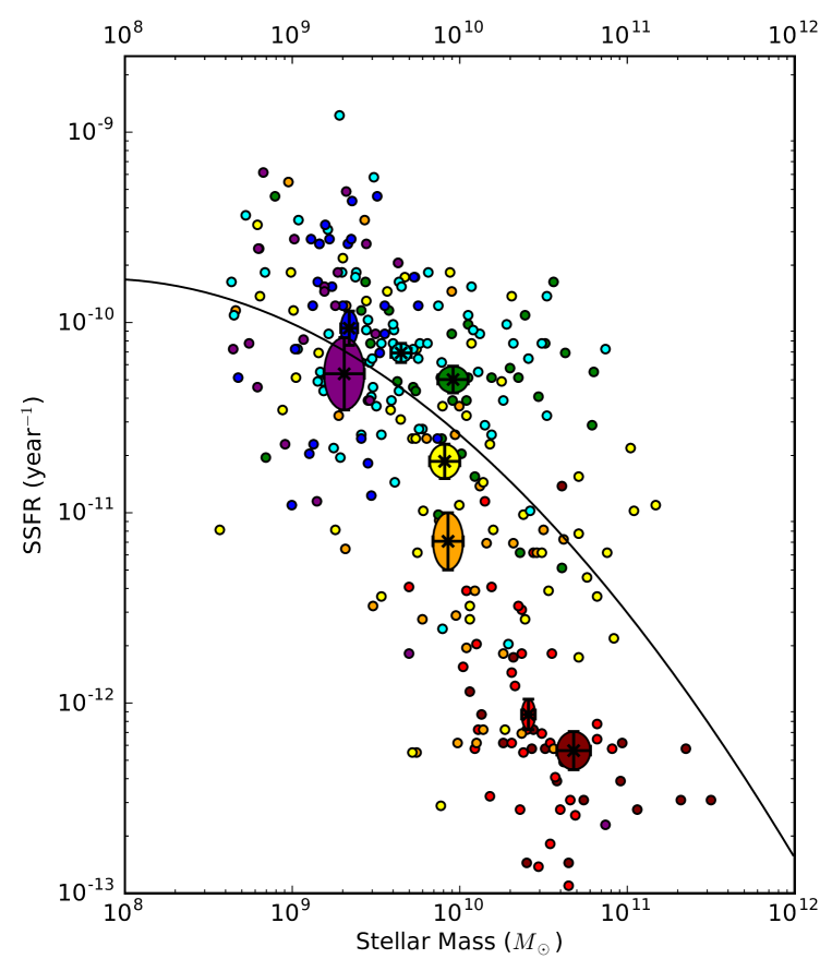
Figure 2: Plot of specific star-formation rate (star-formation rate divided by stellar mass) plotted against galaxy stellar mass. We have used the morphological classification of each galaxy (Boselli et al. 2010) to colour each galaxy point using the following code: maroon - E and E/S0; red - S0; orange - S0a and Sa; yellow - Sab and Sb; green - Sbc; cyan - Sc and Scd; blue - Sd, Sdm; purple - I, I0, Sm and Im. The coloured ellipses show the $1\sigma$ error region on the mean position for each morphological class (Table 1), with the colours being the same as for the individual galaxies. The line is the second-order polynomial that gives the best fit to the data (see text for details) and has the form: $log_{10}SSFR=-10.59-0.76(log_{10}M_{*}-10.0)-0.176(log_{10}M_{*}-10.0)^{2}$.

Before considering the significance of this diagram, there are two key observational issues to consider. The first of these is the completeness of the diagram in terms of galaxy stellar mass. In Appendix A we describe a detailed investigation of the completeness of the HRS for both late-type and early-type galaxies. We show that the HRS will include all galaxies in the HRS volume down to galaxy stellar masses of $\simeq 8\times 10^{8}\ M_{\odot}$ for late-type galaxies and $\simeq 2\times 10^{10}\ M_{\odot}$ for early-type galaxies. Thus the HRS will have missed early-type galaxies in the bottom left-hand corner of Fig. 2. However, there is very little stellar mass in these omitted galaxies, and we show in Appendix A that the mean galaxy stellar mass of the early-type galaxies included in the HRS is very similar to the mean galaxy stellar mass that would have been measured if we had detected all early-type galaxies down to a galaxy stellar masse of $10^{8}\ M_{\odot}$. Three of the four early-type galaxies without MAGPHYS estimates (Section 3) have galaxy stellar masses $>10^{11}\ M_{\odot}$, so their omission will have slightly reduced the mean galaxy stellar mass, offsetting the first effect.

Table 1: Morphological Classes

Morphological	No.	Mean $\rm log_{10}(M_{*})$	Mean $\rm log_{10}(SSFR)$
class
E,ES0	18	10.68$\pm$0.10	-12.25$\pm$0.10
S0	34	10.41$\pm$0.04	-12.06$\pm$0.08
S0a,Sa	32	9.93$\pm$0.09	-11.15$\pm$0.15
Sab,Sb	55	9.91$\pm$0.09	-10.73$\pm$0.09
Sbc	33	9.96$\pm$0.09	-10.30$\pm$0.07
Sc,Scd	70	9.65$\pm$0.06	-10.16$\pm$0.05
Sd,Sdm	29	9.34$\pm$0.05	-10.03$\pm$0.09
Sm,Im,I,I0	22	9.31$\pm$0.12	-10.27$\pm$0.19

The second issue is the accuracy of the specific star-formation rates (SSFR) for galaxies with very low values of SSFR. The median error given by MAGPHYS on $\rm log_{10}(SSFR)$ for galaxies with $\rm-12.0<log_{10}(SSFR)<-11.0$ is 0.23 but increases to 0.39 for galaxies with $\rm log_{10}(SSFR)<-12.0$. The values of SSFR for the galaxies in the lower part of the distribution in Fig. 2 are thus very uncertain. However, in this region of the diagram the distribution of galaxies is almost vertical, and since the estimates of the galaxy stellar mass are much more accurate than the SSFR estimates, it seems unlikely that the large SSFR errors are leading to an erroneous conclusion about the shape of the galaxy distribution. Other methods for estimating the star-formation rate also have great difficulty in providing useful measurements for early-type galaxies with $\rm log_{10}(SSFR)<-12.0$ (e.g. Davis et al. 2014).

There are two things about the diagram that meet the eye. The first is that the galaxy distribution appears curved. To test this statistically, we fitted both a second-order polynomial and a straight line to the points by minimimising the sum of chi-squared in the y-direction. The curve in Fig. 2 is the best-fitting second-order polynomial. The reduction in chi-squared obtained by fitting the polynomial rather than the straight line was $\Delta\chi^{2}\simeq 56$. Since $\Delta\chi^{2}$ is distributed as $\chi^{2}$ with one degree of freedom, the reduction in $\chi^{2}$ obtained from fitting a second-order polynomial rather than a straight line is highly significant, and thus there is strong statistical evidence that the data is better represented by a curve than a straight line. We reached a similar conclusion from minimising $\chi^{2}$ in the x-direction. The distribution in Fig. 2 is not the same as the star-forming main sequence since we have plotted every galaxy in the figure rather than defining a subset of star-forming galaxies. However, we note that there is other evidence that the distribution of galaxies in this diagram is curved, whether only star-forming galaxies are plotted (Whitaker et al. 2014; Lee et al. 2015; Schreiber et al. 2016; Tomczak et al. 2016) or all galaxies are plotted (Gavazzi et al. 2015).

Second, the galaxy morphologies appear to change systematically from the top left to the bottom right of the distribution. To make this clearer, we have calculated the mean values of $\rm log_{10}(SSFR)$ and $\rm log_{10}(stellar\ mass)$ for each morphological class. The values are given in Table 1 and plotted in Figure 2 with their $1\sigma$ error ellipses. The diagram shows that as we move from top left to bottom right along the galaxy distribution we also gradually move along the traditional Hubble sequence.

The HRS volume contains the Virgo Cluster. The HRS does not contain enough galaxies to carry out an investigation of how the properties of the galaxy population depend on environment (e.g. Casado et al. 2015). However, we can investigate whether the trends in Figure 2 are entirely due to the result of the galaxies in Virgo. To do this, we have removed the HRS galaxies whose motions are claimed by Boselli et al. (2010) to be dominated by peculiar motions in Virgo, which consists of the galaxies in Virgo A and B, the north and east clouds and the southern extension. This reduces the HRS by $\simeq 50\%$ to 154 galaxies. In Figure 3 we plot SSFR versus galaxy stellar mass for the remaining galaxies. The same trends are visible.

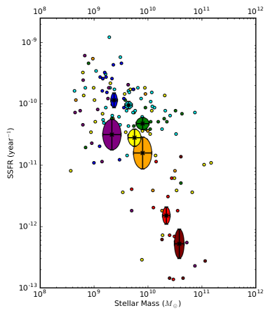
Figure 3: Plot of specific star-formation rate (star-formation rate divided by galaxy stellar mass) plotted against galaxy stellar mass for the galaxies in the HRS outside the Virgo Cluster (see text for details). We have used the morphological classification of each galaxy (Boselli et al. 2010) to colour each galaxy point using the following code: maroon - E and E/S0; red - S0; orange - S0a and Sa; yellow - Sab and Sb; green - Sbc; cyan - Sc and Scd; blue - Sd, Sdm; purple - I, I0, Sm and Im. The coloured ellipses show the $1\sigma$ error region on the mean position for each morphological class with the colours being the same as for the individual galaxies.

We have compared our results with other attempts to plot this diagram using samples from the nearby Universe. In our own investigation we have plotted all galaxies in this diagram rather than defining a subset of star-forming galaxies, which makes it tricky to compare our results with previous investigations of the GMS. Two techniques for defining the star-forming GMS are to select galaxies with an H$\alpha$ equivalent width above some critical value or to select galaxies with colours bluer than some critical value (Speagle et al. 2014). The effect of both criteria is to remove many of the lower points in Figure 2. For example, a critical H$\alpha$ equivalent width of 10Å corresponds to an SSFR of $\rm 3\times 10^{-11}\ year^{-1}$ (Casado et al. 2015), which would remove the bottom half of Figure 2. There is a similar effect with colour cuts. For example, Eales et al. (2016) have plotted this diagram using $\simeq$3000 galaxies selected from the Herschel ATLAS survey, showing that $\simeq$20-30% of the galaxies detected by Herschel would have been classified as ‘passive galaxies’ using optical criteria even though they still have large reservoirs of gas and are still forming stars.

However, there are three recent studies with which we can compare our results. First, Gavazzi et al. (2015) and Eales et al. (2016) have plotted this diagram using samples selected from HI flux and submillimetre flux, respectively, both making no attempt to remove ‘passive galaxies’. Their results are shown in Fig. 4. In both cases, they found a distribution with a similar to shape to what we find here but offset to higher values of SSFR. A possible explanation of the offset is if these two samples are biased toward galaxies with large gas reservoirs and thus larger values of SSFR. Fortunately, we can test this hypothesis because Eales et al. (2016) investigated this effect by fitting a polynomial to their diagram in two ways: not weighting the data points and weighting the datapoints by the inverse of the accessible volume for each galaxy. The two curved lines in Figure 4 show the two fits. Whereas the line from the unweighted fit is offset from our results, the line from the weighted fit follows our distribution well.

The third study is the H$\alpha$ study of Renzini and Peng (2015). The authors attempted to overcome the problem of the rather arbitrary criterion for removing ‘passive galaxies’ by fitting the ridge line of the star-forming main sequence. We have plotted their results over the range of galaxy stellar mass covered by their study, both the relationship they give for the relationship between SSFR and galaxy stellar mass and also one we have recalculated from their relationship using the the recalibration of the relationship between H$\alpha$ luminosity and star-formation rate derived by Davies et al. (2016). The two relationships have a significant offset and have different slopes, showing some of the uncertainty of these studies. Chang et al. (2015) have compared the star-formation rates used by Renzini and Peng with estimates for the same galaxies from MAGPHYS, finding that the latter are lower by $\simeq 0.22$ in $\rm log_{10}(SFR)$, which partly explains the offset between the H$\alpha$ relationship and the HRS points. Another possible explanation for an offset is the rapid low-redshift evolution seen in the Herschel surveys (Dye et al. 2010; Dunne et al. 2011; Eales et al. 2016; Marchetti et al. 2016). Marchetti et al. found that total far-infrared luminosity, which is often used to estimate the star-formation rate of a galaxy (Kennicutt 1998), is proportional to $(1+z)^{6}$. Even though the upper redshift limit of the sample used by Renzini and Peng is only $0.085$, by this redshift, with such rapid evolution, the star-formation rates of galaxies will have increased by $0.21$ in $\rm log_{10}(SFR)$ relative to those in a truly local sample such as the HRS. The combination of the offset between the MAGPHYS and H$\alpha$ estimates of the star-formation rate found by Chang et al. (2015) and the effect of the rapid low-redshift evolution is probably enough to bring the H$\alpha$ GMS into reasonable agreement with the HRS GMS.

Given the uncertainties, there seems reasonable agreement between the different studies of the GMS in the low-redshift Universe.

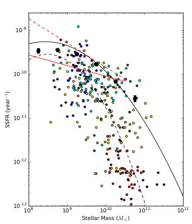
Figure 4: Plot of specific star-formation rate (star-formation rate divided by galaxy stellar mass) plotted against galaxy stellar mass for the galaxies in the HRS. The key for the meaning of the colours of the points is given in the caption to Fig. 2. The large black points show the results for the HI-selected sample of Gavazzi et al. (2015). The solid black line shows the fit to the $\simeq$3000 galaxies selected from the Herschel ATLAS survey (Eales et al. 2016). The dashed line show the fit to the datapoints from the same survey but with the contribution of each galaxy to the fit weighted by the inverse of the galaxy’s accessible volume. The red line shows the fit to the star-forming main sequence from Renzini and Peng (2015). The dashed red line shows the fit for the same sample after it has been recalculated using the recalibration of the relationship between H$\alpha$ luminosity and star-formation rate from Davies et al. (2016).

5 Discussion

Our starting point in this investigation was very different from investigations of the star-forming GMS, because we are interested in what is left in the Universe after $\simeq$12 billion years of star formation rather than in the galaxies producing the stars. We showed in the last section that when a number of obvious and not-so-obvious effects are taken into account, there is fairly good agreement from the different studies of the distribution of galaxies in the plot of galaxy stellar mass versus SSFR in the Universe today. The two clear trends with morphology that are seen in Figure 2, that the specific star-formation rate falls and the galaxy stellar mass rises as one moves along the Hubble sequence from late-type to early-type galaxies, are not new (Devereux and Hameed 1997; Kennicutt 1998; Dressler 2007). The only new things we have done are to show this information on the standard diagram used to interpret galaxy evolution, and to start from a survey that provides a fairly complete census of the stellar mass in the local volume. The main importance of this diagram is that any viable model of galaxy evolution must end up with this distribution of galaxy properties. The main practical limitation of our work is that although we have accurate estimates of the stellar masses of the the early-type galaxies, their star-formation rates are often uncertain. Future observations, in particular with the JWST, will be necessary to delineate the lower part of the distribution.

Galaxy evolution is now often considered in terms of two distinct populations: star-forming and ‘passive galaxies’, which are usually assumed to correspond to late-type galaxies (henceforth LTGs) and early-type galaxies (henceforth ETGs). However, there is no clear evidence for this in Figure 2. There is a possible clump of ETGs in Fig. 2 at $\rm SSFR<10^{-12}\ year^{-1}$ but this is where the values of SSFR are extemely inaccurate, and otherwise there is a gradual change in morphology along the distribution. In H$\alpha$ surveys there is often also often a clump of points around an SSFR of $\rm\simeq 10^{-12}\ year^{-1}$ (e.g. Renzini and Peng 2015), but such values of SSFR correspond to extremely low values of the H$\alpha$ equivalent width ($\sim 1\AA$), and often the clump appears to be a set of upper limits rather than measurements (Renzini and Peng 2015). Establishing whether there are two distinct populations is, of course, of great importance for understanding the physics of galaxy evolution. The existence of two populations is usually explained by a rapid quenching process (e.g. Peng et al. 2010) whereas the existence of a single population with gradually changing properties would require more gentle evolutionary processes.

When one looks in the literature there is a surprising amount of recent evidence for a unitary population of galaxies. For example, Casado et al. (2015), using H$\alpha$ equivalent width as a measure of SSFR and optical luminosity as a measure of galaxy stellar mass, find that field galaxies follow a similar smooth curved distribution to the one we see here (their Figure 8). The ATLAS^3D survey, a volume-limited survey of 260 nearby ETGs similar in many respects to the HRS, has revealed that 86% of ETGs have the velocity field expected for a rotating disk (Emsellem et al. 2011), and for 92% of these ‘fast rotators’ there is also photometric evidence for a stellar disk (Krajnovic et al. 2013). Cappellari et al. (2013) have used the ATLAS^3D results to propose that there is a gradual change in galaxy properties from LTGs to ETGs rather than a dichotomy at the ETG/LTG boundary, with the only exception being the 14% of the ETGs that are ‘slow-rotators’, for which there is generally (but not always) no photometric evidence for a stellar disk (Krajnovic et al. 2013). Cortese et al. (2016), using integral-field spectroscopy from the SAMI survey, have also recently argued that, based on their kinematic properties, LTGs and fast-rotator ETGs form a continuous class of objects.

Other evidence comes from surveys of the interstellar medium (ISM) in ETGs. The ATLAS^3D survey has detected molecular gas in 22% of ETGs (Young et al. 2011), and interferometric observations of the ETGs generally show a rotating disk similar to what is seen in LTGs (Davis et al. 2013). To date, the most sensitive way of detecting the ISM in ETGs has been to use the Herschel Space Observatory to observe the continuum dust emission. Smith et al. (2012) detected dust emission from 50% of the HRS ETGs, and Herschel observations of a much larger sample of ETGs drawn from the ATLAS^3D survey have detected a similar percentage (Smith et al. in preparation). The big increase in detection rate from ground-based CO observations to Herschel observations suggests that the common assumption that ETGs do not contain a cool interstellar medium is largely a function of instrumental sensitivity, and that if we had more sensitive instruments we would find an even higher fraction of ETGs with evidence for a cool ISM. These recent observations of the ISM in ETGs therefore suggest that, although ETGs generally contain less cool gas than LTGs, there is a gradual change in the properties of the cool ISM along the Hubble sequence.

There are two obvious counter-arguments. The first is the claim that the apparent continuity between the ISM properties of ETGs and LTGs is misleading because the gas in ETGs has mostly been acquired as the result of recent mergers. The evidence for this is that $\simeq$24% of ETGs have a difference of $>$30 degrees between the position angles of the stellar and gas rotational axes (Davis et al. 2011). Although this is clearly evidence that some gas in ETGs has been acquired from mergers, in the vast majority of the galaxies in the sample of Davis et al. (33 out of 38) the gas is misaligned by less than 90 degrees, such that the gas rotation vector is still broadly pointing in the same direction as that of the stars (23 of the galaxies have the position angles of the two axes being within 10 degrees of parallel, three have the position angles within 10 degrees of anti-parallel). This suggests that the effect of gas acquired from mergers is mostly to perturb a pre-existing ISM: if the galaxy contained no gas before the merger, the gas rotation vector would have an equal probability of being misaligned by less than and more than 90 degrees. Numerical simulations show that the torque between the acquired gas and the quadrupolar gravitational potential of the stars will eventually bring the two rotational axes into alignment, whether parallel or anti-parallel, but this process acts over long timescales, typically $\sim$2Gyr (van de Voort et al. 2015).

The second counter-argument is that ETGs form a narrow ‘red sequence’ in colour plots (e.g. Bell et al. 2004), suggesting that ETGs form a distinct separate population to LTGs. We show in Appendix B that below a specific star-formation rate of $\rm\simeq 5\times 10^{-12}\ year^{-1}$ the relationship between colour and specific star-formation rate is so weak that, even if galaxies have a uniform distribution of specific star-formation rate, they will still follow a narrow red sequence in colour plots.

Our results and the other recent results described above suggest that late-type galaxies and most early-types (with the possible exception of the 14% of ETGs that are slow rotators) occupy a single continuum. In this picture, a rapid quenching process in which gas is ejected from a late-type galaxy, converting it into a ‘red-and-dead’, ‘passive’, or ‘quiescent’ galaxy, is not required, instead some more gradual evolutionary process, which we will call ‘slow quenching’.

There are other observational results both in favour of and against this hypothesis. Casado et al. (2015) combined H$\alpha$ observations, sensitive to very recent periods of star formation, with optical colours, sensitive to periods of star formation at earlier times, with the aim of looking for sudden changes in the star-formation rate that might indicate rapid quenching. They found no evidence for any such process in low-density environments, although they did find evidence for a rapid quenching process in dense environments. Using a similar technique, Schawinski et al. (2014) found evidence for slow quenching in late-type galaxies but rapid quenching in early-type galaxies. Peng, Maiolino and Cochrane (2015) have used the metallicity distributions of star-forming and quiescent galaxies to argue that the evolution from one population to the other must have occurred over $\simeq$4 billion years - evidence for slow quenching. Schreiber et al. (2016) concluded that at high redshift the decrease in the slope of the star-forming GMS at high galaxy stellar masses can be explained by slow quenching. Although the same problems of measuring accurate values for galaxies with low values of SSFR exist at high redshift, there is some evidence for two distinct populations in the results of Elbaz et al. (2007; their Fig. 17) and of Magnelli et al. (2014; their Fig. 2), supporting rapid quenching. One possible way to reconcile all these results would be if most galaxies evolve by gradual processes (slow quenching) with the 14% of ETGs that are slow rotators being produced by a rapid quenching process.

In summary, we have shown that after 12 billion years of evolution the galaxies in the local volume follow a curved distribution in a plot of SSFR versus galaxy stellar mass, with galaxy morphology changing gradually along this distribution. Any viable theory of galaxy evolution must be able to reproduce the properties of this distribution. Our results and other recent results cast doubt on the idea that there are two distinct populations of galaxies and suggest that most galaxies occupy a single continuum. These results suggest that catastrophic quenching is not required to explain the properties of most of the galaxy population and (to steal a geological term) a more uniformitarian approach is required.

Appendix A How much of the stellar mass in the local volume is contained in the galaxies in the Herschel Reference Survey?

The Herschel Reference Survey consists of 323 galaxies with distances between 15 and 25 Mpc and with a near-infrared K-band limit of $K_{lim}<8.7$ for early-type galaxies (E, S0 and S0a) and $K_{lim}<12$ for late-type galaxies (Sa-Sd-Im-BCD). We have used the following method to estimate how the completeness of the HRS in this volume of space depends on the galaxy stellar mass.

Figure A1 shows the absolute K-band magnitude plotted against the galaxy stellar mass estimate from the MAGPHYS model for the HRS galaxies. The relation is tight and there is no obvious difference in the relationship between early-type and late-type galaxies. The straight line in the figure, which is the best fit to the data and was obtained by minimizing the root-mean-squared-deviations in absolute magnitude, has the following equation:

$$M_{K}=-2.26\times log_{10}(M_{*})+0.07$$ (1)

The completeness of the HRS, $C(M_{*})$, in this volume of space is given by:

$$C(M_{*})={\int^{D_{max}(M_{*})}_{15Mpc}D^{2}dD\over\int^{25Mpc}_{15Mpc}D^{2}dD}$$ (2)

in which $D_{max}(M_{*})$ is the lower of 25 Mpc and $D_{lim}$, where $D_{lim}$ is given by

$$D_{lim}=10^{{K_{lim}-M_{K}(M_{*})-25\over 2.5}}$$ (3)

Figure A2 shows how the completeness of the HRS depends on galaxy stellar mass for late-type galaxies (blue line) and early-type galaxies (red line). The figure shows that the HRS is complete for late-type galaxies for galaxy stellar masses above $\simeq 8\times 10^{8}\ M_{\odot}$ and for early-type galaxies for galaxy stellar masses above $\simeq 2\times 10^{10}\ M_{\odot}$. The implication of the completeness limit for early-type galaxies is that the HRS will have missed early-type galaxies in the lower left-hand corner of Fig. 2.

Is this a big concern? One way to address this question is to consider what fraction of the total mass in the population of early-type galaxies is included in the galaxies detected in the HRS. In making this estimate, we make the assumption that the galaxy stellar mass functions given by Baldry et al. (2012) for optically-red and optically-blue galaxies are appropriate for early-type and late-type galaxies, respectively. Suppose $f(M_{*})$ is the fraction of the total galaxy stellar mass in galaxies with $M>M_{*}$ that is enclosed in the HRS volume and is actually included in the HRS galaxies. This is given by

$$f(M_{*})={\int^{\infty}_{M_{*}}M_{*}\phi(M_{*})\int^{D_{max}(M_{*})}_{15Mpc}D^{2}dDdM_{*}\over\int^{\infty}_{M_{*}}M_{*}\phi(M_{*})dM_{*}\int^{25Mpc}_{15Mpc}D^{2}dD}$$ (4)

in which $\phi(M_{*})$ is the galaxy stellar mass function for either early-type or late-type galaxies.

The results for early-type and late-type galaxies are shown by the dashed red and blue lines in Fig. A2. The figure shows that $\simeq$90% of the total stellar mass in early-type galaxies with galaxy stellar masses $>10^{8}\ M_{\odot}$ is contained in the galaxies actually detected in the HRS. The reason this percentage is so high is because the galaxy stellar mass function for early-type galaxies has a maximum at a galaxy stellar mass of $\simeq 10^{10.5}\ M_{\odot}$, and so even though the HRS completely misses early-type galaxies in the lower left-hand corner of Fig. 2 the actual stellar mass contained in these omitted galaxies is very small.

Another question to ask is whether the horizontal position of the lower part of the galaxy distribution in Fig. 2, the part traced by early-type galaxies, has been biased by the omission of low-mass early-types. To estimate this we have calculated, first, the mean galaxy stellar mass of the early-type galaxies detected in the HRS and then, using the formalism above, the mean mass that we would have measured if we had detected all early-type galaxies with galaxy stellar masses $>10^{8}\ M_{\odot}$. The two vertical lines in Fig. A2 show the two estimates. The lines are very close, showing that the omission of low-mass galaxies has not distorted our perception of the position of the galaxy distribution.

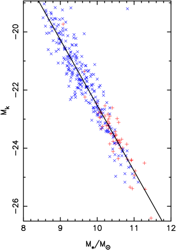
Figure 5: Plot of absolute K-band magnitude versus the galaxy stellar mass estimated from the MAGPHYS model (§3) for the galaxies in the Herschel Reference Survey. The blue crosses represent late-type galaxies and the red crosses early-type galaxies. The equation of the line, which was fit to the points by minimizing the root mean squared deviations in absolute magnitude, is $M_{K}=-2.26\times log_{10}(M_{*})+0.07$.

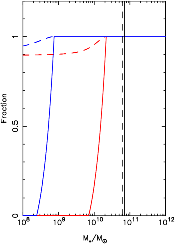
Figure 6: The fraction of galaxies in the HRS volume that are actually included in the HRS plotted against galaxy stellar mass for late-type (solid blue line) and early-type galaxies (solid red line). The dashed lines show the predictions for the fraction of the cumulative galaxy stellar mass (the total galaxy stellar mass above the plotted value) in the HRS volume that is included in the HRS late-type galaxies (dashed blue line) and early-type galaxies (dashed red line). The vertical solid line shows the mean galaxy stellar mass of the early-type galaxies in the HRS; the vertical dashed line shows the predicted mean galaxy stellar mass if the HRS had detected all early-type galaxies with galaxy stellar masses $>10^{8}\ M_{\odot}$.

Appendix B The Cause of the Red Sequence

In this section we show that a population of galaxies that is uniformly distributed in the logarithm of specific star-formation (SSFR) rate will naturally produce a ‘red sequence’ in a colour diagram. We started with a single stellar population from Bruzual and Charlot (2003) with a Salpeter initial mass function and solar metallicity. We then constructed a large number of models for the star-formation history of a galaxy which were designed to produce the full range of SSFR observed in the universe today. These models have no great physical significance and the model from Bruzual and Charlot (1983) was selected fairly randomly, since the goal of the modelling was to see whether a red sequence could be produced even for a uniform distribution in SSFR, not that every possible galaxy-evolution model would produce a red sequence.

Our models of the star-formation history of a galaxy consisted of two sets. In the first set, we assumed that the galaxy formed 12 Gyr ago and that the star-formation rate is proportional to $e^{-{t\over\tau}}$, where $t$ is the time since the formation of the galaxy and $\tau$ is a constant. In this set, we used 1000 values of $\tau$ equally spread logarithmically between 0.5 and 40 Gyr. Since this set could not produce very high values of SSFR, we also constructed a second set of models. In a model in this second set the star-formation history has two components. The first component is an old component, with the exponential form given above and a value of $\tau$ of 40 Gyr. The second component is a burst of star formation that occurs during the last $1.0\times 10^{8}$ years. We constructed a sequence of models, in which the star-formation rate in the burst ranged from 0.01 to $100$ times the star-formation rate at that time in the old component.

Figure 7: Distribution of colour predicted by the models described in the text for a population of galaxies with $log_{10}SSFR$ uniformly spread between -14.0 and -8.5. The solid line shows the predicted distribution for $u-r$ colours and the dashed line for $g-r$ colours.

For each model, we calculated the colour and the SSFR at the current epoch. From the two sets of models, we derived a look-up table linking SSFR and colour. We then assumed a population of galaxies with $\rm log_{10}SSFR$ uniformly spread between -14.0 and -8.5. We then used the look-up table to predict the distribution of colours for this population. Fig. B1 show the predicted distribution of $u-r$ and $g-r$ colour. In both cases, there is a clear red sequence. The explanation of the red sequence is straightforward. Below a SSFR of $\rm\simeq 5\times 10^{-12}\ year^{-1}$, colour depends very weakly on SSFR, so all galaxies below this value of SSFR have virtually the same colour. Therefore, the existence of a red sequence is not a sign of a single homogeneous class of galaxies but merely that there are a large number of galaxies with values of SSFR below this value.

It is worth pointing out that the corresponding colour limit for a young stellar population could have produced a ‘blue sequence’ but in practice does not. The youngest possible population of stars would be one containing only O stars. Such a population would have colours of $u-r\simeq-1.22$ and $g-r\simeq-0.58$. These colours, however, are much bluer than the bluest galaxies in the ‘blue cloud’ (Baldry et al. 2012).

Another way that has been used to show the existence of two distinct populations of galaxies - star-forming and ‘passive’ - is to measure the size of the 4000 Å break from spectra from the Sloan Digital Sky Survey (Kauffmann et al. 2003). Kauffmann et al. used the parameter $D_{n}$, which is the ratio of the average flux density, $F_{\nu}$, in the wavelength range $4000<\lambda<4100\ \AA$ to the average flux density in the wavelength range $3850<\lambda<3950\ \AA$. Galaxies fall nicely into two distinct areas on a plot of $D_{n}$ verses stellar mass (see Fig. 1 of Kauffmann et al.). We repeated our modelling in exactly the same way as before except that this time we calculated the relationship between SSFR and $D_{n}$. Figure B2 shows the predicted distribution of $D_{n}$ for a population of galaxies with $\rm log_{10}SSFR$ uniformly spread between -14.0 and -8.5. There is a clear peak, again a consequence of the weak dependence between $D_{n}$ and SSFR below a value of SSFR of $\rm\simeq 2\times 10^{-12}\ year^{-1}$.

Figure 8: Distribution of the strength of the 4000 Å break predicted by the models described in the text for a population of galaxies with $log_{10}SSFR$ uniformly spread between -14.0 and -8.5.

References

- Abramson et al. (2016) Abramson, L.E. et al. 2016, arXiv:1604.00016
- Baldry et al. (2012) Baldry, I.K. et al. (2012), MNRAS, 441, 2440
- Bell et al. (2004) Bell, E.F. et al. 2004, ApJ, 608, 752
- Bendo et al. (2012) Bendo, G., Galliano, F. & Madden, S.C. 2012, MNRAS, 423, 197
- Boselli et al. (2010) Boselli, A. et al. 2010, PASP, 122, 261
- Bournaud et al. (2007) Bournaud, F., Elmgreen, B.G. & Elmgreen, D.M. 2007, ApJ, 670, 237
- Bruzual and Charlot (2003) Bruzual, G. & Charlot, S. 2003, MNRAS, 344, 1000
- Cappellari et al. (2013) Cappellari, M. et al. 2013, MNRAS, 432, 1862
- Casado et al. (2015) Casado, J., Acasibar, Y., Gavilan, M., Terlevich, R., Terlevich, E., Hoyos, C. & Diaz, A.I. 2015, MNRAS, 451, 888
- Chabrier (2003) Chabrier, G. 2003, PASP, 115, 763
- Chang et al. (2015) Chang, Y.-Y., van der Wel, A., Da Cunha, E. & Rix, H.-W. 2015, ApJ suppl. 219, 8
- Ciesla et al. (2012) Ciesla, L. et al. 2012, A&A, 543, 161
- Ciesla et al. (2014) Ciesla, L. et al. 2014, A&A, 565, 128
- Cortese et al. (2012a) Cortese, L. et al. 2012a, A&A, 544, 101
- Cortese et al. (2012b) Cortese, L. et al. 2012b, A&A, 540, 52
- Cortese et al. (2014) Cortese, L. et al. 2014, MNRAS, 440, 942
- Cortese et al. (2016) Cortese, L. et al. 2016, MNRAS, 463, 170
- Da Cunha et al. (2008) Da Cunha, E., Charlot, S. and Elbaz, D. 2008, MNRAS, 388, 1595
- Daddi et al. (2007) Daddi, E. et al. 2007, ApJ, 670, 156
- Davies et al. (2016) Davies, L.J.M. et al. 2016, MNRAS, 461, 458
- Davis et al. (2011) Davis, T.A. et al. 2011, MNRAS, 417, 882
- Davis et al. (2013) Davis, T.A. et al. 2013, MNRAS, 429, 534
- Davis et al. (2013) Davis, T.A. et al. 2014, MNRAS, 444, 3427
- De Vis et al. (2016) De Vis, P. et al. 2016, MNRAS, in press (arXiv: 1610.01038)
- Devereux and Hameed (2007) Devereux, N.A. and Hameed, S. 1997, AJ, 113, 599
- Dressler (2007) Dressler, A. 2007, From Stars to Galaxies: Building the Pieces to Build Up the Universe, ASP Conference Series, 374, 415
- Dunne et al. (2011) Dunne, L. et al. 2011, MNRAS, 417, 1510
- Dye et al. (2010) Dye, S. et al. 2010, AA, 518, L10
- Eales et al. (2015) Eales, S.A. et al. 2015, MNRAS, 452, 3489
- Eales et al. (2016) Eales, S.A. et al. submitted to MNRAS
- Elbaz et al. (2007) Elbaz, D. et al. 2007, A&A, 468, 33
- Emsellem et al. (2011) Emsellem, E. et al. 2011, MNRAS, 414, 888
- Gavazzi et al. (2015) Gavazzi, G. et al. 2015, A&A, 580, 116
- Genzel et al. (2011) Genzel, R. et al. 2011, ApJ, 733, 30
- Genzel et al. (2014) Genzel, R. et al. 2014, ApJ, 785, 75
- Genzel et al. (2015) Genzel, R. et al. 2015, ApJ, 800, 20
- Gladders et al. (2013) Gladders, M.D. et al. 2013, ApJ, 770, 64
- Kauffmann (2003) Kauffmann, G. et al. (2003), MNRAS, 341, 54
- Kennicutt (1998) Kennicutt, R.C. 1998, ARAA, 36, 189
- Krajnovic et al. (2013) Krajnovic, D. et al. 2013, MNRAS, 432, 1768
- Lang et al. (2014) Lang, P. et al. 2014, ApJ, 788, L11
- Lee et al. (2015) Lee, N. et al. 2015, ApJ, 801, 80
- Magnelli (2014) Magnelli, B. et al. 2014, A&A, 561, 86
- Marchetti et al. (2016) Marchetti, L. et al. 2016, MNRAS, 456, 1999
- Noguchi (1999) Noguchi, M. 1999, ApJ, 514, 77
- Noeske et al. (2007) Noeske, K.G. et al. 2007, ApJ, 660, L43
- Pannella et al. (2009) Pannella, M. et al. 2009, ApJ, 701, 787
- Papadopoulos and Geach (2012) Papadopoulos, P. and Geach, J.E. 2012, ApJ, 757, 157
- Peng et al. (2010) Peng, Y.-J. et al. 2010, ApJ, 721, 193
- Peng et al. (2015) Peng, Y., Maiolino, R. & Cochrane, R. 2015, Nature, 521, 192
- Pilbratt et al. (2010) Pilbratt, G. et al. 2010, A&A, 518, L1
- Planck Collaboration (2014) Planck Collaboration 2014, A&A, 571, 26
- Popescu et al. (2011) Popescu, C.C., Tuffs, R.J., Dopita, M.A., Fischera, J., Kylafis, N.D. and Madore, B.F. 2011, A&A, 527, 109
- Renzini and Peng (2015) Renzini, A. & Peng, Y. 2015, ApJ, 801, L29
- Rodighiero et al. (2011) Rodighiero, G. et al. 2011, ApJ, 739, 40
- Rowlands et al. (2014) Rowlands, K. et al. 2014, MNRAS, 441, 1017
- Santini et al. (2014) Santini, P. et al. 2014, A&A, 562, 30
- Schawinski et al. (2014) Schawinski, K. et al. 2014, MNRAS, 440, 889
- Schreiber et al. (2016) Schreiber, C. et al. 2016, A&A, 589, 35
- Scoville et al. (2016) Scoville, N. et al. 2016, ApJ, 820, 83
- Sheth et al. (2010) Sheth, K. et al. PASP, 122, 1397
- Skrutskie et al. (2006) Skrutskie, M.F. et al. 2006, AJ, 131, 1163
- Smith et al. (2012) Smith, M.W.L. et al. 2012, ApJ, 748, 123
- Speagle et al. (2014) Speagle, J.S., Steinhardt, C.L., Capak, P.L. & Silverman, J.D. 2014, ApJS, 214, 15
- Tacconi et al. (2010) Tacconi, L. et al. 2010, Nature, 463, 781
- Tomczak et al. (2016) Tomczak, A. et al. 2016, ApJ, 817, 118
- Toomre (1977) Toomre, A. 1977, Evolution of Galaxies and Stellar Populations, Proceedings of a Conference at Yale University, edited by B.M. Tinsley and R.B. Larson (Yale University Observatory, New Haven, Conn.), 401
- van de Voort et al. (2015) van der Voort, F. et al. 2011, MNRAS, 451, 3269
- Wang et al. (2016) Wang, L. et al. 2016, MNRAS, submitted
- Whitaker et al. (2012) Whitaker, K. et al. 2012, ApJ, 754, 29
- Whitaker et al. (2014) Whitaker, K. et al. 2014, ApJ, 795, 104
- Whitaker et al. (2015) Whitaker, K. et al. 2015, ApJ, 811, L12
- Wuyts et al. (2011) Wuyts, S. et al. 2011, ApJ, 742, 20
- Young et al. (2011) Young, L.M. et al. 2011, MNRAS, 414, 940
- Zibetti et al. (2009) Zibetti, S., Charlot, S. & Rix, H.-W. 2009, MNRAS, 400, 1181