1 Introduction

The existence of a Dark Matter (DM) component of the Universe is confirmed by several astrophysical and cosmological probes, e.g. the CMB [1] and structure formation. Particle physics solutions to the DM problem mostly rely on the existence of a new particle that is stable on cosmological scales thanks to a symmetry, and with weak enough interactions with Standard Model (SM) states to evade constraints from direct and indirect searches. From the model-building point of view, these requirements are naturally satisfied by a “hidden” sector whose states are singlets with respect to the SM symmetry group. In this kind of a setup, stable particles of the hidden sector are Dark Matter candidates.

Despite the different symmetry groups acting on the visible and hidden sectors, renormalizable interactions can arise among them. The dimension–4 operators relevant to our study are obtained by combining the gauge invariant dimension two terms $H^{\dagger}H$ and $B^{\mu\nu}$ with similar dimension-two operators formed by the states of the hidden sector. The strength of such “portal” interactions can be sufficient to bring the visible and hidden sectors in thermal equilibrium in the Early Universe and realize the WIMP paradigm. In addition, the DM candidates retain interactions with the visible particles at present times, which could be within the reach of the current and future searches for new particles.

In the simplest models of this type, the hidden sector is populated (effectively) by a single field which constitutes DM. The lowest order Higgs portal operators mediating interactions between the DM and the SM states then read $H^{\dagger}H|\chi|^{2}$ or $H^{\dagger}HV^{\mu}V_{\mu}$, with $\chi$ and $V^{\mu}$ being a scalar and a vector DM candidate, respectively, see e.g. [2, 3, 4, 5, 6, 7, 8, 9]. These simple set–ups are currently under pressure from constantly improving experimental constraints. Indeed, by crossing symmetry arguments, there is a relation between the DM pair annihilation cross-section at freeze-out, responsible for the relic density, and the processes potentially responsible for detection signals, such as scattering on nuclei, probed by Direct Detection experiments, or production at colliders. Null results of the latter then rule out large portions of the parameter space favoured by the thermal WIMP paradigm [15, 16]. If the s-wave DM annihilation cross section remains substantial at present times, the model can also be probed by Indirect Detection experiments. These considerations motivate exploration of richer hidden sector structures. For example, additional annihilation channels into dark sector states can deplete the DM relic density without changing its interactions with the visible sector while satisfying the experimental constraints [17, 18].

More generally, there is no a priori reason for the DM of the Universe to be composed of a single field. Multi-component DM frameworks, with two or more particles contributing a non-negligible fraction to the total relic density $\Omega_{\rm DM,\rm tot}h^{2}\approx 0.12$, offer interesting perspectives. The relation between the annihilation cross section and the current detection signals has to be properly reconsidered. Some work in this direction has been carried out in [20, 19], where the discovery potential of the current and future experimental facilities and the capability of discriminating multicomponent DM from single–component DM have been studied. We note that multicomponent DM emerges in various particle physics models (see e.g. [21, 22, 23, 24]).

In this work, we will investigate multicomponent DM emerging from a hidden sector endowed with gauge symmetry. Such systems enjoy natural discrete symmetries which can act as DM stabilizers. Indeed, it was noted in [6] and detailed in [8] that a hidden sector consisting of a U(1) gauge field $A_{\mu}$ and a single complex scalar which breaks the symmetry spontaneously has the symmetry

$$Z_{2}~{}:~{}~{}~{}A_{\mu}\rightarrow-A_{\mu}\;.$$ (1)

As a result, the massive vector field $A_{\mu}$ is stable and can constitute DM. This idea generalizes to non–Abelian gauge symmetries as well. In particular, hidden SU(N) sectors with a minimal matter content necessary to break the gauge symmetry completely, that is $N-1$ scalar $N$-plets, are endowed with a $Z_{2}\times Z_{2}^{\prime}$ symmetry [25]

$$Z_{2}~{}:~{}~{}~{}A_{\mu}^{a}\rightarrow(-1)^{n_{a}}A_{\mu}^{a}\;,$$

$$Z_{2}^{\prime}~{}:~{}~{}~{}A_{\mu}^{a}\rightarrow(-1)^{n_{a}^{\prime}}A_{\mu}^{a}\;,$$ (2)

where $A_{\mu}^{a}$ is the gauge field, $a$ is the adjoint group index and $n_{a},n_{a}^{\prime}$ take on values 0,1 depending on $a$. One of the $Z_{2}$’s corresponds to complex conjugation of the SU(N) group elements, while the other is a gauge transformation. In the SU(2) case, the symmetry enlarges in fact to custodial SO(3) [6] (see also [26, 27]), while for larger groups it is part of a global unbroken $U(1)\times Z_{2}^{\prime}$. Since the SM fields are neutral under the above symmetries, $A_{\mu}^{a}$ cannot decay into the visible sector particles and therefore can constitute dark matter. Note that since the symmetry is $Z_{2}\times Z_{2}^{\prime}$, one expects at least $two$ different DM components, in contrast to traditional $Z_{2}$–invariant WIMP models. The exact composition depends on the details of the spectrum. In particular, the SU(3) example studied in [25] has only vector DM with two components being degenerate in mass and the third one being somewhat lighter. These states interact with the visible sector through the Higgs portal operators. A related study has recently appeared in [28].

In our current study, we explore a qualitatively different case of mixed spin DM, that is containing both spin 1 and spin 0 components. We employ the model of [25] in a different parametric regime, where a stable pseudoscalar is lighter than the gauge field with the same $Z_{2}\times Z_{2}^{\prime}$ quantum numbers. In this case, the pseudoscalar as well as the gauge fields with distinct $Z_{2}\times Z_{2}^{\prime}$ quantum numbers constitute DM. The resulting phenomenology is very different from that of [25]. In particular, we find that there are substantial regions of parameter space where the direct detection cross section is suppressed.

We stress that although we study a specific model of multicomponent DM, many of the results presented here are of general relevance. In particular, depending on the composition of DM, the direct detection signal strength varies drastically, over orders of magnitude, and is often consistent with thermal relic DM abundance. Such behaviour is specific to more complicated hidden sectors within our framework and reflects the possibility that common models may oversimplify the DM properties.

One of the novel aspects of our study is that multicomponent DM is a natural consequence of our UV–complete framework, due to $Z_{2}\times Z_{2}^{\prime}$ being part of the Yang–Mills symmetries. This is in contrast to more conventional models where the two DM components have different origins such as the mixed axion–neutralino DM scenario [29, 30]. Consequently, the contributions of the components to the total DM density are controlled by a set of the UV parameters. In our study, much emphasis will be given to the analysis of the DM production processes (as opposed to the approach of [20, 19]). We solve numerically the coupled Boltzmann equations and calculate the individual relic abundances as a function of the parameters of the model. The composition of DM can be very different in different parameter regions and in some of them both DM components give comparable contributions. We then study the Direct Detection constraints and observe an interesting effect. As long as the SM Higgs mixes predominantly with one of the hidden scalar fields, the direct detection is highly suppressed in the parameter regions where DM is mostly spin-0. It can be so small that even future detectors like XENON1T [31] will not be able to probe it. This is one of the main results of our study.

The paper is structured as follows. The model is introduced in Section 2. Section 3 is devoted to a detailed discussion of the relic DM density calculations and the Direct Detection limits. We also comment on the possibility of detecting one of the components through Indirect Detection. Our results are summarized in Section 4.

2 The SU(3) hidden sector model

The purpose of this section is to briefly summarise our model, mostly following Ref. [25]. The hidden sector of the model is endowed with SU(3) gauge symmetry, which is broken spontaneously (to nothing) by two hidden triplets $\phi_{1}$ and $\phi_{2}$. This is the minimal setup that allows one to make all the SU(3) gauge fields massive.

The Lagrangian of the model is

$${\cal L}_{\rm SM}+{\cal L}_{\rm portal}+{\cal L}_{\rm hidden}\;,$$ (3)

where

$$-{\cal L}_{\rm SM} \supset V_{\rm SM}=\frac{\lambda_{H}}{2}|H|^{4}+m_{H}^{2}|H|^{2}\;,$$ (4a)

$$-{\cal L}_{\rm portal} =V_{\rm portal}=\lambda_{H11}\,|H|^{2}|\phi_{1}|^{2}+\lambda_{H22}\,|H|^{2}|\phi_{2}|^{2}-(\lambda_{H12}\,|H|^{2}\phi_{1}^{\dagger}\phi_{2}+{\textrm{h.c.}})\;,$$ (4b)

$${\cal L}_{\rm hidden} =-\frac{1}{2}\textrm{tr}\{G_{\mu\nu}G^{\mu\nu}\}+|D_{\mu}\phi_{1}|^{2}+|D_{\mu}\phi_{2}|^{2}-V_{\rm hidden}\,.$$ (4c)

Here, $G_{\mu\nu}=\partial_{\mu}A_{\nu}-\partial_{\nu}A_{\mu}+i\tilde{g}[A_{\mu},A_{\nu}]$ is the field strength tensor of the SU(3) gauge fields $A_{\mu}^{a}$ with gauge coupling $\tilde{g}$, $D_{\mu}\phi_{i}=\partial_{\mu}\phi_{i}+i\tilde{g}A_{\mu}\phi_{i}$ is the covariant derivative of $\phi_{i}$, $H$ is the Higgs doublet, which in the unitary gauge can be written as $H^{T}=(0,v+h)/\sqrt{2}$, and the most general renormalisable hidden sector scalar potential is given by

$$V_{\rm hidden}(\phi_{1},\phi_{2}) =m_{11}^{2}|\phi_{1}|^{2}+m_{22}^{2}|\phi_{2}|^{2}-(m_{12}^{2}\phi_{1}^{\dagger}\phi_{2}+{\textrm{h.c.}})$$

$$+\frac{\lambda_{1}}{2}|\phi_{1}|^{4}+\frac{\lambda_{2}}{2}|\phi_{2}|^{4}+\lambda_{3}|\phi_{1}|^{2}|\phi_{2}|^{2}+\lambda_{4}|\phi_{1}^{\dagger}\phi_{2}|^{2}$$

$$+\left[\frac{\lambda_{5}}{2}(\phi_{1}^{\dagger}\phi_{2})^{2}+\lambda_{6}|\phi_{1}|^{2}(\phi_{1}^{\dagger}\phi_{2})+\lambda_{7}|\phi_{2}|^{2}(\phi_{1}^{\dagger}\phi_{2})+{\textrm{h.c.}}\right]\,.$$ (5)

The fields $\phi_{1}$ and $\phi_{2}$ are responsible for the spontaneous breaking of the hidden SU(3) symmetry. In the unitary gauge, they can be written as

$$\phi_{1}={1\over\sqrt{2}}\,\left(\begin{array}[]{c}0\\ 0\\ v_{1}+\varphi_{1}\end{array}\right)\,,\quad\phi_{2}={1\over\sqrt{2}}\,\left(\begin{array}[]{c}0\\ v_{2}+\varphi_{2}\\ v_{3}+\varphi_{3}+i\varphi_{4}\end{array}\right)~{},$$ (6)

where the $v_{i}$ are real VEVs and $\varphi_{i}$ are real scalar fields. Here we assume the $CP$ symmetry in the scalar sector, i.e. that the couplings are real and $\varphi_{4}$ attains no VEV. As a consequence there is no mixing between the CP-even scalar fields $\varphi_{1-3}$ and the CP-odd scalar $\varphi_{4}$. This allows for the possibility that $\varphi_{4}$ is stable.

A minor technical complication that occurs in this model is that the quadratic part of the Lagrangian is not diagonal, due to the mixing terms

$$\mathcal{L}\supset\frac{\tilde{g}v_{2}}{2}A^{\mu\,6}\partial_{\mu}\varphi_{4}-\frac{\tilde{g}v_{3}}{\sqrt{3}}A^{\mu\,8}\partial_{\mu}\varphi_{4}+\frac{\tilde{g}v_{3}}{2}A^{\mu\,7}\partial_{\mu}\varphi_{2}-\frac{\tilde{g}v_{2}}{2}A^{\mu\,7}\partial_{\mu}\varphi_{3}\,.$$ (7)

These terms of the form $\kappa_{ai}A_{\mu}^{a}\partial^{\mu}\varphi^{i}$ can be removed by the transformation

$$A^{a}_{\mu}\rightarrow\tilde{A}^{a}_{\mu}=A^{a}_{\mu}+\partial_{\mu}Y^{a},\quad\textrm{with}\quad Y^{a}\equiv(\mathcal{M})^{-1}_{ab}\kappa_{bi}\varphi_{i}\,,$$ (8)

where $\mathcal{M}$ is the mass matrix of the hidden gauge bosons. This leaves $\mathcal{M}$ unchanged. After the above transformation the kinetic terms of the $\varphi_{i}$ are not canonically normalised anymore so that a further transformation

$$\varphi_{i}\rightarrow\tilde{\varphi}^{i}=\omega_{ik}\varphi^{k}\;,\quad\textrm{where}\quad(\omega^{T}\omega)_{ij}\equiv\delta_{ij}-\kappa^{T}_{ia}{\cal M}^{-1}_{ab}\kappa_{bj}\,,$$ (9)

is needed to make the quadratic part of the Lagrangian canonically normalised. To stress its special role as a DM candidate, we relabel

$$\chi\equiv\tilde{\varphi}_{4}\,.$$ (10)

To simplify the analysis, in the rest of the paper we assume that the couplings $m_{12}^{2},\lambda_{H12},\lambda_{6},\lambda_{7}$ in the scalar potential, as well as the VEV $v_{3}$, are small but non-vanishing. If they did vanish, the system would attain an additional unwanted $Z_{2}$ symmetry $\phi_{2}\rightarrow-\phi_{2}$, which would lead to extra stable particles and change the phenomenology of the model. In the limit of small $v_{3}$, the only gauge-scalar mixing terms are $A^{\mu\,6}\partial_{\mu}\varphi_{4}$ and $A^{\mu\,7}\partial_{\mu}\varphi_{3}$ so that $\tilde{\varphi}_{1}\simeq\varphi_{1}$ and $\tilde{\varphi}_{2}\simeq\varphi_{2}$.

The mass matrix for the (pseudo)scalar fields reads:

$$-\mathcal{L}\supset\frac{1}{2}\Phi^{T}m_{\mathrm{{\it CP}-even}}^{2}\Phi+\frac{1}{4}\left(\lambda_{4}-\lambda_{5}\right)(v_{1}^{2}+v_{2}^{2})\chi^{2},$$ (11)

where $\Phi=(h,\varphi_{1},\varphi_{2},\tilde{\varphi_{3}})^{T}$. In the limit $v_{3}\ll v_{1},v_{2}$, we get

$$m_{\mathrm{{\it CP}-even}}^{2}=\left(\begin{array}[]{cccc}\lambda_{H}v^{2}&\lambda_{H11}vv_{1}&\lambda_{H22}vv_{2}&0\\ \lambda_{H11}vv_{1}&\lambda_{1}v_{1}^{2}&\lambda_{3}v_{1}v_{2}&0\\ \lambda_{H22}vv_{2}&\lambda_{3}v_{1}v_{2}&\lambda_{2}v_{2}^{2}&0\\ 0&0&0&(\lambda_{4}+\lambda_{5})(v_{1}^{2}+v_{2}^{2})/2\end{array}\right).$$ (12)

We see that $\tilde{\varphi}_{3}$ does not mix with the other states and is a mass eigenstate. The other mass eigenstates are obtained by diagonalising the upper $3\times 3$ sub-matrix. For further simplification, we will assume that the (1,2) and (2,3) entries of $m_{\mathrm{{\it CP}-even}}^{2}$ are much smaller than the other matrix elements, which can be achieved with sufficiently small $\lambda_{H11}$ and $\lambda_{3}$. Then $\varphi_{1}$ is approximately a mass eigenstate, which we call ${\cal H}$ (to be consistent with the notation in Ref. [25]), and $m_{{\cal H}}^{2}=\lambda_{1}v_{1}^{2}$. The other two mass eigenstates are

$$h_{1}\simeq c_{\theta}h-s_{\theta}\varphi_{2}~{},$$

$$h_{2}\simeq s_{\theta}h+c_{\theta}\varphi_{2}~{},$$ (13)

with

$$m_{h_{1},h_{2}}^{2}\simeq\frac{1}{2}\left(\lambda_{2}v_{2}^{2}+\lambda_{H}v^{2}\right)\mp\frac{\lambda_{2}v_{2}^{2}-\lambda_{H}^{2}v^{2}}{2c_{2\theta}}~{},$$

$$\tan 2\theta\simeq\frac{2\lambda_{H22}vv_{2}}{\lambda_{2}v_{2}^{2}-\lambda_{H}^{2}v^{2}}\,.$$ (14)

The eigenstate $h_{1}$ is identified with the 125 GeV Higgs boson and, consequently, its couplings are required to be SM-like. This translates into the requirement $s_{\theta}\lesssim 0.3$ (see e.g. [32]).

We now turn to the vectors. In the limit $v_{3}\ll v_{1},v_{2}$ the vector sector is composed of 6 pure states which form 3 mass degenerate pairs with masses

$$m_{A^{1}}^{2}=m_{A^{2}}^{2}=\frac{\tilde{g}^{2}}{4}v_{2}^{2},\quad m_{A^{4}}^{2}=m_{A^{5}}^{2}=\frac{\tilde{g}^{2}}{4}v_{1}^{2},\quad m_{A^{6}}^{2}=m_{A^{7}}^{2}=\frac{\tilde{g}^{2}}{4}(v_{1}^{2}+v_{2}^{2})\,,$$ (15)

and two mixed eigenstates

$$A_{\mu}^{3\,^{\prime}}=A_{\mu}^{3}\cos\alpha+A_{\mu}^{8}\sin\alpha~{},$$

$$A_{\mu}^{8\,^{\prime}}=A_{\mu}^{8}\cos\alpha-A_{\mu}^{3}\sin\alpha~{},$$ (16)

where

$$\alpha=\left\{\begin{array}[]{ll}\frac{1}{2}\arctan\left(\frac{\sqrt{3}v_{2}^{2}}{2v_{1}^{2}-v_{2}^{2}}\right)&\textrm{for}\quad v_{2}^{2}\leq 2v_{1}^{2}\vspace{5pt}\\ \frac{1}{2}\arctan\left(\frac{\sqrt{3}v_{2}^{2}}{2v_{1}^{2}-v_{2}^{2}}\right)+\frac{\pi}{2}&\textrm{for}\quad v_{2}^{2}>2v_{1}^{2}~{},\end{array}\right.$$ (17)

so that $\alpha\in(0^{\circ},60^{\circ})$. The masses are

$$m_{A^{3\,^{\prime}}}^{2}=\frac{\tilde{g}^{2}v_{2}^{2}}{4}\left(1-\frac{\tan\alpha}{\sqrt{3}}\right),\,\,\,\,\,m_{A^{8\,^{\prime}}}^{2}=\frac{\tilde{g}^{2}v_{1}^{2}}{3}\frac{1}{1-\frac{\tan\alpha}{\sqrt{3}}}\,.$$ (18)

Our setup enjoys a $Z_{2}\times Z^{{}^{\prime}}_{2}$ symmetry (cf. Eq. (2)). The $Z_{2}^{\prime}$ acts as complex conjugation, which is an outer automorphism of SU(3), while the $Z_{2}$ is a gauge transformation that acts non–trivially only on the upper entry of the SU(3) triplets. They are inherent in the Yang–Mills system and remain unbroken by interactions with matter in our minimal setting.

This discrete symmetry is in fact part of a global $U(1)\times Z_{2}^{\prime}$ preserved by the vacuum. The global U(1)

$$U=e^{i\beta/3}\;{\rm diag}(e^{-i\beta},1,1)$$ (19)

is a subgroup of the SU(3) hidden gauge symmetry and acts on the gauge fields as $A_{\mu}\to UA_{\mu}U^{\dagger}$. This corresponds to $(A_{1,4},A_{2,5})\to(\cos\beta A_{1,4}-\sin\beta A_{2,5},\sin\beta A_{1,4}+\cos\beta A_{2,5})$ and leaves $A_{3,6,7,8}$ invariant. The scalar sector Eq. (5) possesses an independent global U(1)^′ symmetry $\phi_{1,2}\to e^{i\gamma}\;\phi_{1,2}$. Since $U$ acts effectively as an overall phase transformation on the scalar fields of the form Eq. (6), the vacuum preserves a combination of U(1) and U(1)^′. This symmetry ensures, for instance, that $m_{A_{1}}=m_{A_{2}}$ and $m_{A_{4}}=m_{A_{5}}$ (see [25]).

Although the unbroken symmetry is $U(1)\times Z_{2}^{\prime}$, for our purposes it suffices to consider its subgroup $Z_{2}\times Z^{{}^{\prime}}_{2}$. The corresponding charges are given in Table 1.

gauge eigenstates	mass eigenstates	$Z_{2}\times Z_{2}^{\prime}$
$h,\varphi_{1-3},A_{\mu}^{7}$	$h_{1,2},{\cal H},{\tilde{\varphi}}_{3},\tilde{A}_{\mu}^{7}$	$(+,+)$
$A_{\mu}^{1},A_{\mu}^{4}$	$A_{\mu}^{1},A_{\mu}^{4}$	$(-,-)$
$A_{\mu}^{2},A_{\mu}^{5}$	$A_{\mu}^{2},A_{\mu}^{5}$	$(-,+)$
$\varphi_{4},A_{\mu}^{3},A_{\mu}^{6},A_{\mu}^{8}$	$\chi,A_{\mu}^{\prime 3},\tilde{A}_{\mu}^{6},A_{\mu}^{\prime 8}$	$(+,-)$

Table 1: $Z_{2}\times Z_{2}^{\prime}$ charges of the scalars and hidden vectors.

The lightest vector state is always $A^{3\,^{\prime}}$. It is however not necessarily stable since $|D_{\mu}\phi_{2}|^{2}$ generates the coupling

$${\cal L}\supset(1+r)\frac{\tilde{g}}{\sqrt{3}}\sin\alpha\left(\chi A_{\mu}^{3\,^{\prime}}\partial^{\mu}\tilde{\varphi}_{3}-\chi\leftrightarrow\tilde{\varphi}_{3}\right)~{},$$ (20)

where

$$r\equiv v_{2}^{2}/v_{1}^{2}\,,$$ (21)

allowing for the decay $A^{3\,^{\prime}}\rightarrow\chi+{\tilde{\varphi}_{3}}\rightarrow\chi+{\rm SM}$ if $m_{A^{3\,^{\prime}}}>m_{\chi}$. Here ${\tilde{\varphi}_{3}}$ is produced off-shell and leads to the SM final states since the coupling of ${\tilde{\varphi}_{3}}$ to $h_{1},h_{2}$ is nonzero for $v_{3}\neq 0$.

The masses of $A^{3\,^{\prime}}$ and $\chi$ are related by

$$\frac{m_{\chi}^{2}}{m^{2}_{A^{\prime 3}}}=\frac{\lambda_{4}-\lambda_{5}}{\tilde{g}^{2}}f(r)\,,\quad\textrm{with}\quad f(r)=\frac{3(r+1)}{r+1-\sqrt{1+r(r-1)}}\,.$$ (22)

The decay $A^{3\,^{\prime}}\rightarrow\chi$ + SM is thus kinematically open if $\lambda_{4}-\lambda_{5}<\tilde{g}^{2}/f(r)$. For $r$ around unity, one has $f(r)=6+\mathcal{O}((1-r)^{2})$, while for $r\ll 1$, $f(r)\simeq 2/r+\mathcal{O}(1)$. If one requires $\chi$ to be part of DM, relatively small $\tilde{g}$ necessitates therefore very small $\lambda_{4}-\lambda_{5}$.

In summary, our SU(3) hidden sector adds to the particle content the following states: 8 massive vector bosons, three scalars $h_{2},{\cal H},\tilde{\varphi}_{3}$ and one pseudo-scalar $\chi$. Given the charges under the $Z_{2}\times Z_{2}^{{}^{\prime}}$ symmetry and the mass relations of Eqs. (15,18,22), different states can contribute to Dark Matter. The options are summarized in Table 2. In all cases, DM consists of 3 states. Since $A_{1},A_{2}$ are degenerate in mass, one may introduce a formal analog of the $W^{\pm}$ bosons via the linear combinations $A_{1}\pm iA_{2}$ even though $A_{1},A_{2}$ have different parities. We find that such a redefinition facilitates numerical computations, in particular, what concerns the software Micromegas. This allows for the treatment of $A_{1},A_{2}$ as an effectively single (complex) DM component. A similar redefinition can be applied to another mass degenerate pair $A_{4},A_{5}$ .

	Case I	Case II	Case III	Case IV
parameter	$v_{2}<v_{1}$	$v_{2}>v_{1}$	$v_{2}<v_{1}$	$v_{2}>v_{1}$
choice	$\lambda_{4}-\lambda_{5}$ small	$\lambda_{4}-\lambda_{5}$ small	$\lambda_{4}-\lambda_{5}\geq\mathcal{O}(1)$	$\lambda_{4}-\lambda_{5}\geq\mathcal{O}(1)$
dark matter	$A_{\mu}^{1}$,$A_{\mu}^{2}$,$\chi$	$A_{\mu}^{4}$,$A_{\mu}^{5}$,$\chi$	$A_{\mu}^{1}$,$A_{\mu}^{2}$,$A_{\mu}^{\prime 3}$	$A_{\mu}^{4}$,$A_{\mu}^{5}$,$A_{\mu}^{\prime 3}$

Table 2: DM composition for different parameter choices (cf. Eq. (22)).

The four possible cases can be understood as follows. For $v_{2}<v_{1}$ ($v_{1}<v_{2}$) the degenerate pair $A_{1,2}$ ($A_{4,5}$) is stable, because these are the lightest states with a given non–trivial $Z_{2}\times Z_{2}^{{}^{\prime}}$ charge. The only possible decay would be of the type $A_{1}\rightarrow A_{2}A_{3}$ which is kinematically forbidden. The other stable state of the hidden sector is either $\chi$ or $A^{3\,^{\prime}}$, depending on the value of $\lambda_{4}-\lambda_{5}$. The purely vectorial DM case was studied in [25]. In this work, we will instead focus on case I, with mixed scalar–vector DM.

3 Multicomponent Dark Matter Phenomenology

Many of the important features of our model can be obtained by taking the limit $v_{1}\gg v_{2}$. This reduces the number of states relevant to DM phenomenology to the DM candidates $A_{1,2}$ and $\chi$, two mediators $h_{1}$ and $h_{2}$, and the state $A_{3}$ whose mass is between that of $A_{1,2}$ and $\chi$. We discuss this limit in the next subsection. Afterwards, we also consider the case $v_{1}\simeq v_{2}$ where all hidden states play a role and highlight the differences between these two limits.

3.1 Case $v_{1}\gg v_{2}$

For $v_{1}\gg v_{2}$, the mass scales of $A_{1,2}$,$A^{{}^{\prime}}_{3}$ on one hand and $A_{4-7},A^{{}^{\prime}}_{8}$ on the other hand are split, with the latter being higher by a factor of order $v_{1}/v_{2}$. The same happens in the scalar sector where the states ${\cal H},{\tilde{\varphi}}_{3}$ are parametrically heavier than $h_{1,2}$. On the other hand, since we are interested in a relatively light $\chi$, we take a small enough value of $\lambda_{4}-\lambda_{5}$ to keep its mass below that of $A^{{}^{\prime}}_{3}$ (cf. Eq. (22)). In practice, $v_{1}/v_{2}\simeq 3-5$ is sufficiently large to neglect the heavier states, while we take $v_{1}/v_{2}=10$ in our numerical studies.

For $v_{1}\gg v_{2}(\gg v_{3})$, the relevant for our purposes Lagrangian is given by

$$\mathcal{L}=\mathcal{L}_{\rm DM}+\mathcal{L}_{\scriptscriptstyle h\text{-}\rm SM\text{-}SM}+\mathcal{L}_{h\text{-}h\text{-}h}\;,$$ (23)

where we neglect the $h^{4}$–type couplings which do not contribute significantly to the DM relic density computations. Here, the DM Lagrangian, containing the mass terms and the $h_{1},h_{2}$ interaction terms, is

$$\mathcal{L}_{\rm DM} =\frac{1}{2}m_{A}^{2}\sum_{a=1,2}A^{a}_{\mu}A^{a\mu}-\frac{1}{2}m_{\chi}^{2}\chi^{2}$$ (24)

$$+\left[\frac{\tilde{g}\,m_{A}}{2}\left(-h_{1}s_{\theta}+h_{2}c_{\theta}\right)+\frac{\tilde{g}^{2}}{8}\left(h_{1}^{2}s^{2}_{\theta}-2h_{1}h_{2}s_{\theta}c_{\theta}+h_{2}^{2}c^{2}_{\theta}\right)\right]\sum_{a=1,2}A^{a}_{\mu}A^{a\mu}$$

$$+\left[\frac{\tilde{g}(1+r)}{2m_{A}}\left(-h_{1}s_{\theta}m_{h_{1}}^{2}+h_{2}c_{\theta}m_{h_{2}}^{2}\right)-\frac{1}{4}\left(\lambda_{\chi\chi 11}h_{1}^{2}+2\lambda_{\chi\chi 12}h_{1}h_{2}+\lambda_{\chi\chi 22}h_{2}^{2}\right)\right]\chi^{2}\,,$$

where

$$\lambda_{\chi\chi 11} =(1+r)\frac{\tilde{g}}{2m_{A}v}s_{\theta}\left(c^{3}_{\theta}(m_{h_{2}}^{2}-m_{h_{1}}^{2})+\frac{\tilde{g}v}{2m_{A}}s_{\theta}(s^{2}_{\theta}m_{h_{1}}^{2}+c^{2}_{\theta}m_{h_{2}}^{2})\right)~{},$$ (25a)

$$\lambda_{\chi\chi 12} =(1+r)\frac{\tilde{g}}{2m_{A}v}s_{\theta}c_{\theta}\left(s_{\theta}c_{\theta}(m_{h_{2}}^{2}-m_{h_{1}}^{2})-\frac{\tilde{g}v}{2m_{A}}(s^{2}_{\theta}m_{h_{1}}^{2}+c^{2}_{\theta}m_{h_{2}}^{2})\right)~{},$$ (25b)

$$\lambda_{\chi\chi 22} =(1+r)\frac{\tilde{g}}{2m_{A}v}c_{\theta}\left(s^{3}_{\theta}(m_{h_{2}}^{2}-m_{h_{1}}^{2})+\frac{\tilde{g}v}{2m_{A}}c_{\theta}(s^{2}_{\theta}m_{h_{1}}^{2}+c^{2}_{\theta}m_{h_{2}}^{2})\right)\,.$$ (25c)

The couplings of $h_{1}$ and $h_{2}$ to SM matter are given by

$$\mathcal{L}_{\scriptscriptstyle h\text{-}\rm SM\text{-}SM}={h_{1}c_{\theta}+h_{2}s_{\theta}\over v}\left[2m_{W}^{2}W_{\mu}^{+}W^{\mu-}+m_{Z}^{2}Z_{\mu}Z^{\mu}-\sum_{f}m_{f}\bar{f}f\right]\,.$$ (26)

The remaining term ${\cal L}_{h\text{-}h\text{-}h}$ represents the trilinear couplings among $h_{1}$ and $h_{2}$,

$${\cal L}_{h\text{-}h\text{-}h}=-{\kappa_{111}\over 6}v~{}h_{1}^{3}-{\kappa_{112}\over 2}v~{}h_{1}^{2}h_{2}-{\kappa_{221}\over 2}v~{}h_{2}^{2}h_{1}-{\kappa_{222}\over 6}v~{}h_{2}^{3}~{},$$ (27)

where

$$\kappa_{111} ={3m_{h_{1}}^{2}\over v^{2}}\left(c^{3}_{\theta}-s^{3}_{\theta}\frac{\tilde{g}v}{2m_{A}}\right)~{},$$ (28a)

$$\kappa_{112} ={2m_{h_{1}}^{2}+m_{h_{2}}^{2}\over v^{2}}s_{\theta}c_{\theta}\left(c_{\theta}+s_{\theta}\frac{\tilde{g}v}{2m_{A}}\right)~{},$$ (28b)

$$\kappa_{221} ={m_{h_{1}}^{2}+2m_{h_{2}}^{2}\over v^{2}}s_{\theta}c_{\theta}\left(s_{\theta}-c_{\theta}\frac{\tilde{g}v}{2m_{A}}\right)~{},$$ (28c)

$$\kappa_{222} ={3m_{h_{2}}^{2}\over v^{2}}\left(s^{3}_{\theta}+c^{3}_{\theta}\frac{\tilde{g}v}{2m_{A}}\right)~{}\,.$$ (28d)

Note that the quartic couplings $\lambda_{H},\lambda_{2},\lambda_{H22}$ do not explicitly appear in the above interaction terms since they are fixed in terms of $v,m_{h_{1}},m_{h_{2}},\sin\theta,\tilde{g}$ and $m_{A}$:

$$\lambda_{H}=\frac{c^{2}_{\theta}m_{h_{1}}^{2}+s^{2}_{\theta}m_{h_{2}}^{2}}{v^{2}}~{},$$

$$\lambda_{2}=\tilde{g}^{2}\frac{s^{2}_{\theta}m_{h_{1}}^{2}+c^{2}_{\theta}m_{h_{2}}^{2}}{4m_{A}^{2}}~{},$$

$$\lambda_{H22}=\tilde{g}s_{2\theta}\frac{m_{h_{2}}^{2}-m_{h_{1}}^{2}}{4vm_{A}}\,.$$ (29)

The couplings in Eq. (23) therefore are a function of the 5 new physics parameters $m_{\chi},m_{A},m_{h_{2}},\tilde{g},\sin\theta$. The hidden sector gauge coupling $\tilde{g}$ acts as an overall normalization parameter for the DM interactions.

In what follows, we analyze how the DM relic density is generated as well as the constraints and prospects for Direct DM Detection.

3.1.1 Relic density

In conventional WIMP scenarios, the DM relic density is inversely proportional to the thermally averaged DM annihilation cross-section into SM fermions. In the case of multicomponent DM, the situation is more involved since there are additional important processes such as conversion of one DM component into another. This complicates the analysis and we therefore solve the system of Boltzmann equations numerically (cf. [17, 33, 28]).

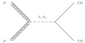
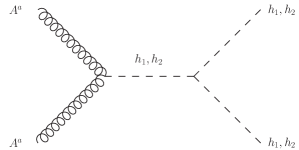
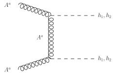
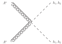
Figure 1: Pair annihilation processes for the vectorial DM component.

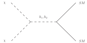
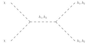
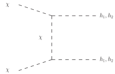
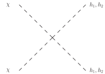
Figure 2: Pair annihilation processes for the scalar DM component.

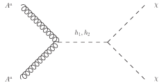
Figure 3: Vector DM to scalar DM conversion.

The Boltzmann equations are dictated by three types of processes:

• Pair annihilation of both DM components into SM fermions, gauge and Higgs bosons

• Conversion of one DM component into another: $AA\leftrightarrow\chi\chi$

• Semi–(co)annihilation (cf. [34, 35]): $AA\rightarrow A_{3}h_{1,2}$ and $AA_{3}\rightarrow Ah_{1,2}$ which changes the abundances of both the vector and the scalar component

The relevant diagrams for the annihilation processes of the two DM components are presented in Figs. 1-3, while the (subleading) semi–annihilation processes are not shown explicitly. The Boltzmann equations can be written as

$$\frac{dY_{A}}{dx} =-\overline{\langle\sigma v\rangle}_{AA\rightarrow XX}\left(Y_{A}^{2}-Y_{A,\rm eq}^{2}\right)-\overline{\langle\sigma v\rangle}_{AA\rightarrow\chi\chi}\left(Y_{A}^{2}-\frac{Y_{A,\rm eq}^{2}}{Y_{\chi,\rm eq}^{2}}Y_{\chi}^{2}\right)$$ (30)

$$\qquad-\overline{\langle\sigma v\rangle}_{AA\rightarrow A_{3}h_{1,2}}\left(Y_{A}^{2}-\frac{Y_{\chi}}{Y_{\chi,\rm eq}}Y^{2}_{A,\rm eq}\right),$$

$$\frac{dY_{\chi}}{dx} =-\overline{\langle\sigma v\rangle}_{\chi\chi\rightarrow XX}\left(Y_{\chi}^{2}-Y_{\chi,\rm eq}^{2}\right)+\overline{\langle\sigma v\rangle}_{AA\rightarrow\chi\chi}\left(Y_{A}^{2}-\frac{Y_{A,\rm eq}^{2}}{Y_{\chi,\rm eq}^{2}}Y_{\chi}^{2}\right)$$

$$\qquad-\overline{\langle\sigma v\rangle}_{AA_{3}\rightarrow Ah_{1,2}}Y_{A}Y_{A_{3},\rm eq}\left(\frac{Y_{\chi}}{Y_{\chi,\rm eq}}-1\right)+\overline{\langle\sigma v\rangle}_{AA\rightarrow A_{3}h_{1,2}}\left(Y_{A}^{2}-\frac{Y_{\chi}}{Y_{\chi,\rm eq}}Y^{2}_{A,\rm eq}\right),$$

where $Y_{i}=n_{i}/s$ with $n_{i}$ being the corresponding number density and $s$ being the entropy, $x=m_{A}/T$ and

$$\overline{\langle\sigma v\rangle}(x)=\frac{\langle\sigma v\rangle s}{Hx}\Big{|}_{T=m_{A}/x}\,,$$ (31)

where $H$ is the Hubble rate.

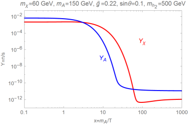
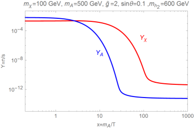
Figure 4: Solutions of the Boltzmann equations for two benchmark parameter values. In each panel, the red and blue curves represent the abundances of the $\chi$ and $A$ DM components, respectively.

The resulting evolution of the yields $Y_{i}$ for two benchmark parameter choices is shown in Fig. 4. In the right panel, the relic density of the two components evolves similarly to that of conventional WIMPs, i.e. it tracks the equilibrium distribution at Early times until decoupling. In the left panel, we see some modifications to this behaviour. In particular, the pseudoscalar DM components annihilates very efficiently through the $h_{1}$ resonance which depletes its energy density, while at late times the $\chi$ fraction of the DM number density increases due to the conversion process of Fig. 3. In this case, the heavier DM component gives the dominant contribution to the DM density.

Our numerical analysis (see below for more details) shows that the contribution of the processes $AA\rightarrow A_{3}h_{1,2}$ and $AA_{3}\rightarrow Ah_{1,2}$ is negligible over most of the parameter space. For a qualitative discussion of our numerical results, one may thus approximate the total DM relic density by the sum of the following two contributions [37],

$$\Omega_{\rm DM,tot}h^{2} \approx 8.8\times 10^{-11}\,{\mbox{GeV}}^{-2}\left[{\left(\bar{g}_{\rm eff,A}^{1/2}\int_{T_{0}}^{T_{f,A}}\!\!\langle\sigma v\rangle_{A}\frac{dT}{m_{A}}\right)}^{-1}\!\!\!\!+{\left(\bar{g}^{1/2}_{\rm eff,\chi}\int_{T_{0}}^{T_{f,\chi}}\!\!\langle\sigma v\rangle_{\chi}\frac{dT}{m_{\chi}}\right)}^{-1}\right]$$

$$\approx 8.8\times 10^{-11}\,{\mbox{GeV}}^{-2}\left[\frac{x_{f,A}}{\bar{g}_{\rm eff,A}^{1/2}\left(a_{A}+x_{f,A}^{-1}b_{A}\right)}+\frac{x_{f,\chi}}{\bar{g}_{\rm eff,\chi}^{1/2}\left(a_{\chi}+x_{f,\chi}^{-1}b_{\chi}\right)}\right],$$ (32)

where $T_{f,\chi},T_{f,A}$ are the freeze-out temperatures of the two DM components, $T_{0}$ is the present time temperature and $g_{\rm eff,A,\chi}$ are the effective degrees of freedom in the Early Universe. In the second line of Eq. (3.1.1), we have used the velocity expansion $\langle\sigma v\rangle\simeq a+2b/x$ (using $\sigma v\simeq a+bv^{2}/3$ and $\langle v^{2}\rangle=6/x$, cf. e.g. [38]) and $x_{f,i}=m_{i}/T_{f,i}$.

In this work we only consider the case $m_{\chi}<m_{A}$ as required by our model. Indeed, $A_{3}$ is always lighter than $A_{1,2}$ with our SU(3) breaking mechanism and $\chi$ must be lighter than $A_{3}$ to be stable. Hence, we include the conversion process $AA\rightarrow\chi\chi$, but not the reverse (at least at late times).

The relevant annihilation cross-sections are s-wave dominated, i.e. the coefficients $a_{\chi,A}$ are not suppressed. At leading order in velocity expansion, they read

• Pseudoscalar component:

  $$\langle\sigma v\rangle_{\chi\chi\rightarrow\bar{f}f}= \sum_{f}\frac{\tilde{g}^{2}N_{c}^{f}}{4\pi v^{2}}s^{2}_{2\theta}\ {\left(1-\frac{m_{f}^{2}}{m_{\chi}^{2}}\right)}^{3/2}\frac{m_{f}^{2}m_{\chi}^{4}{\left(m_{h_{1}}^{2}-m_{h_{2}}^{2}\right)}^{2}}{{m_{A}^{2}\left(m_{h_{1}}^{2}-4m_{\chi}^{2}\right)}^{2}{\left(m_{h_{2}}^{2}-4m_{\chi}^{2}\right)}^{2}}~{},$$

  $$\langle\sigma v\rangle_{\chi\chi\rightarrow W^{+}W^{-}}= \frac{\tilde{g}^{2}}{2\pi v^{2}}s^{2}_{2\theta}\sqrt{1-\frac{m_{W}^{2}}{m_{\chi}^{2}}}\left(1-\frac{m_{W}^{2}}{m_{\chi}^{2}}+\frac{3}{4}\frac{m_{W}^{4}}{m_{\chi}^{4}}\right)\times$$

  $$\quad\frac{{m_{\chi}^{6}\left(m_{h_{1}}^{2}-m_{h_{2}}^{2}\right)}^{2}}{{m_{A}^{2}\left(m_{h_{1}}^{2}-4m_{\chi}^{2}\right)}^{2}{\left(m_{h_{2}}^{2}-4m_{\chi}^{2}\right)}^{2}}~{},$$

  $$\langle\sigma v\rangle_{\chi\chi\rightarrow ZZ}= \frac{\tilde{g}^{2}}{4\pi v^{2}}s^{2}_{2\theta}\sqrt{1-\frac{m_{Z}^{2}}{m_{\chi}^{2}}}\left(1-\frac{m_{Z}^{2}}{m_{\chi}^{2}}+\frac{3}{4}\frac{m_{Z}^{4}}{m_{\chi}^{4}}\right)\times$$

  $$\quad\frac{{m_{\chi}^{6}\left(m_{h_{1}}^{2}-m_{h_{2}}^{2}\right)}^{2}}{{m_{A}^{2}\left(m_{h_{1}}^{2}-4m_{\chi}^{2}\right)}^{2}{\left(m_{h_{2}}^{2}-4m_{\chi}^{2}\right)}^{2}}~{}.$$ (33)

• Vector component:

  $$\langle\sigma v\rangle_{AA\rightarrow\bar{f}f}= \sum_{f}\frac{\tilde{g}^{2}N_{c}^{f}}{48\pi v^{2}}s^{2}_{2\theta}{\left(1-\frac{m_{f}^{2}}{m_{A}^{2}}\right)}^{3/2}\frac{{m_{f}^{2}m_{A}^{2}\left(m_{h_{1}}^{2}-m_{h_{2}}^{2}\right)}^{2}}{{\left(m_{h_{1}}^{2}-4m_{A}^{2}\right)}^{2}{\left(m_{h_{2}}^{2}-4m_{A}^{2}\right)}^{2}}~{},$$

  $$\langle\sigma v\rangle_{AA\rightarrow W^{+}W^{-}}= \frac{\tilde{g}^{2}}{24\pi v^{2}}s^{2}_{2\theta}\sqrt{1-\frac{m_{W}^{2}}{m_{A}^{2}}}\left(1-\frac{m_{W}^{2}}{m_{A}^{2}}+\frac{3}{4}\frac{m_{W}^{4}}{m_{A}^{4}}\right)\times$$

  $$\frac{{m_{A}^{4}\left(m_{h_{1}}^{2}-m_{h_{2}}^{2}\right)}^{2}}{{\left(m_{h_{1}}^{2}-4m_{A}^{2}\right)}^{2}{\left(m_{h_{2}}^{2}-4m_{A}^{2}\right)}^{2}}$$

  $$\langle\sigma v\rangle_{AA\rightarrow ZZ}= \frac{\tilde{g}^{2}}{48\pi v^{2}}s^{2}_{2\theta}\sqrt{1-\frac{m_{Z}^{2}}{m_{A}^{2}}}\left(1-\frac{m_{Z}^{2}}{m_{A}^{2}}+\frac{3}{4}\frac{m_{Z}^{4}}{m_{A}^{4}}\right)\times$$

  $$\frac{{m_{A}^{4}\left(m_{h_{1}}^{2}-m_{h_{2}}^{2}\right)}^{2}}{{\left(m_{h_{1}}^{2}-4m_{A}^{2}\right)}^{2}{\left(m_{h_{2}}^{2}-4m_{A}^{2}\right)}^{2}}~{},$$

  $$\langle\sigma v\rangle_{AA\rightarrow\chi\chi}= \frac{\tilde{g}^{4}}{768\pi m_{A}^{2}}\sqrt{1-\frac{m_{\chi}^{2}}{m_{A}^{2}}}\times$$

  $$\frac{{\left(m_{h_{1}}^{2}m_{h_{2}}^{2}-2m_{A}^{2}(m_{h_{1}}^{2}+m_{h_{2}}^{2})+2m_{A}^{2}(m_{h_{1}}^{2}-m_{h_{2}}^{2})c_{2\theta}\right)}^{2}}{{\left(m_{h_{1}}^{2}-4m_{A}^{2}\right)}^{2}{\left(m_{h_{2}}^{2}-4m_{A}^{2}\right)}^{2}}\,.$$ (34)

The “dark” annihilation process $AA\rightarrow\chi\chi$ can be the most efficient $A$–annihilation channel since it is not suppressed by $\sin^{2}2\theta$, which is subject to rather tight experimental constraints [32]. This is because the process involves only the dark sector states. As a result, the annihilation cross-section of the vector DM component is often enhanced compared to that of the scalar component.

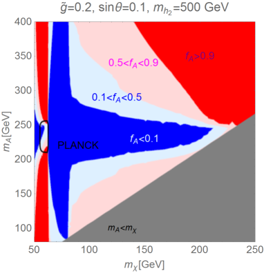
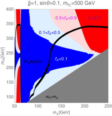
Figure 5: The ratio $f_{A}=\Omega_{A}/\Omega_{\rm tot}$ in the $(m_{\chi},m_{A})$-plane, for $\sin\theta=0.1$, $m_{h_{2}}=500~{}{\rm GeV}$ and $\tilde{g}=0.2$ (left) respectively $\tilde{g}=1$ (right). The blue, light blue, light red and red regions correspond to $f_{A}<0.1$, $0.1<f_{A}<0.5$, $0.5<f_{A}<0.9$ and $f_{A}>0.9$, respectively. In the black regions, the observed total DM relic density is correctly reproduced at the 3 $\sigma$ level.

In Fig. 5, we show the contribution of the vector component to the total DM relic density, $f_{A}=\Omega_{A}/\Omega_{\rm DM,tot}$, in the plane $(m_{\chi},m_{A})$ with fixed $\tilde{g}$, $s_{\theta}$ and $m_{h_{2}}$. We distinguish the following three regions: $f_{A}<0.1$ (blue), $0.1<f_{A}<0.5$ (light blue), $0.5<f_{A}<0.9$ (light red) and $f_{A}>0.9$ (red). The correct DM relic density is only reproduced in the black regions, so the purpose of the plot is to help understand how the composition of DM evolves as a function of parameters.

Since the total DM relic density is given approximately by Eq. (3.1.1) and $x_{f,A}\approx x_{f,\chi}$, $\sqrt{\bar{g}_{\rm eff,A}}\approx\sqrt{\bar{g}_{\rm eff,\chi}}$, $f_{A}$ mostly depends on the ratio of the pair annihilation cross-sections of the two DM components:

$$f_{A}\approx\frac{\frac{\langle\sigma v\rangle_{\chi}}{\langle\sigma v\rangle_{A}}}{1+\frac{\langle\sigma v\rangle_{\chi}}{\langle\sigma v\rangle_{A}}}\;.$$ (35)

An obvious feature of Fig. 5, which follows immediately from the above equation, is that the $A_{\mu}$ DM component dominates when $\chi$ annihilates resonantly, and vice versa. For the regions away from the resonances, a closer inspection of $\frac{\langle\sigma v\rangle_{\chi}}{\langle\sigma v\rangle_{A}}$ is required.

Let us identify qualitative features of $\frac{\langle\sigma v\rangle_{\chi}}{\langle\sigma v\rangle_{A}}$. For the mass range shown in the plot, $\langle\sigma v\rangle_{\chi}$ is dominated by $\langle\sigma v\rangle_{\chi\chi\rightarrow\bar{b}b}$ for $m_{W}>m_{\chi}$ and by $\langle\sigma v\rangle_{\chi\chi\rightarrow WW}$ for $m_{W}<m_{\chi}$. $\langle\sigma v\rangle_{A}$ has contributions from annihilation to both dark and visible sector final states. Which one dominates depends mostly on the ratio $\tan\theta/\tilde{g}$. For instance, one has

$$\frac{\langle\sigma v\rangle_{AA\to W^{+}W^{-}}}{\langle\sigma v\rangle_{AA\to\chi\chi}}=8\frac{\tan^{2}\theta}{\tilde{g}^{2}}\frac{m^{2}_{A}}{v^{2}}\left(1-\frac{m_{\chi}^{2}}{m_{A}^{2}}\right)^{-1/2}\times\left(1+\mathcal{O}\left(\frac{m_{W}^{2}}{m_{A}^{2}},\frac{m_{h_{1}}^{2}}{4m_{A}^{2}},\frac{m_{h_{1}}^{2}}{m_{h_{2}}^{2}}\right)\right).$$ (36)

The ratio $\frac{\langle\sigma v\rangle_{AA\to\bar{b}b}}{\langle\sigma v\rangle_{AA\to\chi\chi}}$ has an additional $m_{b}^{2}/m_{\chi}^{2}$ suppression factor.

• From Eq. (36) we see that in the right plot, where $\tilde{g}\gg\sin\theta$, the dark annihilation $AA\to\chi\chi$ dominates in most mass regions. An exception is the region where $A_{\mu}$ is not much heavier than $\chi$ so that the dark annihilation is phase-space suppressed.

  • For $m_{\chi}>m_{W}$, the ratio $\frac{\langle\sigma v\rangle_{\chi}}{\langle\sigma v\rangle_{A}}$ becomes

    $$\frac{\langle\sigma v\rangle_{\chi\chi\rightarrow W^{+}W^{-}}}{\langle\sigma v\rangle_{AA\rightarrow\chi\chi}} =$$ (37)

    $$\!\!\!\!\!\!\!\!\!\!96\frac{\tan^{2}\theta}{\tilde{g}^{2}}\frac{m^{2}_{\chi}}{v^{2}}\frac{{\left(m_{h_{2}}^{2}-4m_{A}^{2}\right)}^{2}}{{\left(m_{h_{2}}^{2}-4m_{\chi}^{2}\right)}^{2}}\left(1+\mathcal{O}\left(\frac{m_{W}^{2}}{m_{\chi}^{2}},\frac{m_{h_{1}}^{2}}{4m_{\chi}^{2}},\frac{m_{h_{1}}^{2}}{m_{h_{2}}^{2}},\frac{m_{\chi}^{2}}{m_{A}^{2}}\right)\right).$$

    For most parameter ranges of interest, the $A_{\mu}$ annihilation cross section is much larger than that for $\chi$. As a result, $f_{A}<0.1$. This does not however apply to the region $m_{A}^{2}\gg m_{h_{2}}^{2}/4$ (upper part of the plot) in which case the factor $(2m_{A}/m_{h_{2}})^{4}$ can compensate the small ratio $(\tan\theta/\tilde{g})^{2}$.

  • For $m_{\chi}<m_{W}$, the $\chi$ annihilation cross section is suppressed by the $b$–quark mass. The resulting $\frac{\langle\sigma v\rangle_{\chi}}{\langle\sigma v\rangle_{A}}$ and $f_{A}$ are small unless $\chi$ annihilates resonantly.

• In the left plot, $\sin\theta$ and $\tilde{g}$ have similar sizes so that the visible and dark $A_{\mu}$ annihilation channels play in general comparable roles. Two features are clearly visible: resonant $A_{\mu}$ annihilation or $b$–quark mass suppression of $\langle\sigma v\rangle_{\chi}$ for $m_{W}>m_{\chi}$ lead to small $f_{A}$.

We find that the correct relic DM density typically requires sizable $\tilde{g}$ and $s_{\theta}$. If $\tilde{g}$ is too small, the $\chi$ DM component is overproduced. As seen in Fig. 5, at $\tilde{g}=0.2$ one must resort to resonant $\chi$ annihilation to keep its density under control. The DM composition is very sensitive to the exact $\chi$–mass in this case. With a larger gauge coupling, $\tilde{g}=1$, the correct relic density is achieved in substantial regions of parameter space. We find numerically that both DM components can be as heavy as a few hundred GeV, while $\tilde{g}s_{\theta}\gtrsim 0.01$ is required to keep the $\chi$–annihilation efficient. While qualitative features of the plot can be understood semi-analytically, we have performed our numerical analysis using the software Micromegas [39] which is well suited for 2 component DM.

In Fig. 6, we show the contours of correct DM relic density in the $(m_{A},\tilde{g})$-plane (left panels) and $(m_{\chi},\tilde{g})$-plane (right panels). The color coding along the contours indicates the value of $f_{A}$: the red (blue) end of the spectrum refers to vector (pseudoscalar) dominance.

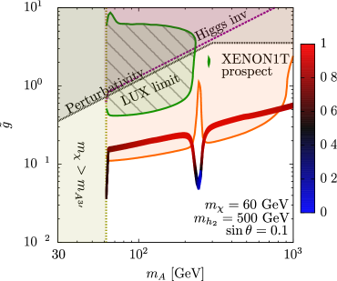
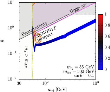
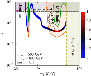
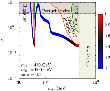
Figure 6: Dark matter constraints in the plane $(m_{A},\tilde{g})$ (upper panel) and $(m_{\chi},\tilde{g})$ (lower panel) for $v_{1}\gg v_{2}$. The blue–red band indicates the correct relic DM density with the blue (red) end of the spectrum referring to the spin-0 (spin-1) component dominance. The other curves mark the following constraints: grey – perturbativity, purple – invisible Higgs decay, green – LUX 2016 direct DM detection, orange – XENON1T direct DM detection prospects.

Many features of the plots can be understood qualitatively. In the upper left panel, the dark annihilation process $AA\rightarrow\chi\chi$ is important, yet the resulting $\chi$ states annihilate very efficiently through the $h_{1}$ resonance into the SM fields. As a result, DM is mostly vector (apart from the small region $m_{A}\simeq m_{h_{2}}/2$). The necessary $\tilde{g}$ at $\sin\theta=0.1$ is smaller than that in [25] due to the availability of the dark annihilation channel, albeit it remains in the same ballpark of ${\cal O}(10^{-1})$. In the right upper panel, the $\chi$ mass moves a bit further from the center of the $h_{1}$ resonance, which changes the DM composition and requires somewhat larger gauge couplings. Nevertheless, the resonance is still efficient and allows one to obtain the correct relic density with a relatively small $\tilde{g}$.

In the lower panels, the relic density band has the resonant structure similar to that of [25]. The narrow $h_{1}$ resonance at $m_{\chi}\simeq m_{h_{1}}/2$ is followed by a much broader resonance around $m_{h_{2}}/2$. The kinks in the band represent new annihilation channels becoming kinematically available, e.g. $\chi\chi\rightarrow h_{1}h_{1}$. In most regions away from the tip of the resonance, DM is predominantly pseudoscalar.

Besides the prospects for direct detection, which will be discussed in the following subsection, Fig. 6 displays the limits from perturbativity of the quartic ($\lambda_{i}<4\pi$) and gauge ($\tilde{g}^{2}_{i}<4\pi$) couplings as well as those from the invisible decay of the 125 GeV Higgs boson. While the former has almost no impact on the region with the correct DM relic density, the latter excludes light values of $m_{\chi}$ below approximately 50 GeV.

3.1.2 Direct detection

In this subsection, we discuss the limits from the LUX experiment [40], as well as prospects for direct detection in XENON1T [31]. The interactions of the pseudoscalar and vector DM components with nuclei are vastly different, thus it is convenient to discuss them separately.

• Scattering of the $\chi$ component:
   
  The spin–independent (SI) $\chi$–nucleon scattering cross-section vanishes at tree-level in the limit of low momentum transfer:

  $$\sigma_{\chi N}\simeq 0\,.$$ (38)

  Thus, the pseudoscalar DM component appears to hide from detection albeit in a different manner compared to the known mechanisms which rely on the pseudo-scalar/axial-vector mediators [41, 42]. The reason for it is a cancellation between the $t$–channel $h_{1}$ and $h_{2}$ contributions which follows from the coupling

  $${\cal L}\supset(1+r)\frac{\tilde{g}}{2m_{A}}\left(-h_{1}m_{h_{1}}^{2}s_{\theta}+h_{2}m_{h_{2}}^{2}c_{\theta}\right)\chi^{2}$$ (39)

  as well as the $h_{1},h_{2}$ couplings to SM matter.

  Since this is an important feature of this model, let us discuss the origin of this ‘blind’ spot in the $\chi$–$N$ scattering in more detail. To this end, let us consider now the $\chi$–nucleon interaction the interaction basis, i.e. before diagonalising the scalar mass matrix. The pseudoscalar $\chi$ interacts with the scalars $\varphi_{1}$ and $\varphi_{2}$ of the dark sector and $h$ of the Standard Model, while only the latter couples to quarks. In the interaction basis, the effective $\chi\chi NN$ coupling is

  $$g_{\chi\chi NN}=(\vec{\kappa}_{\chi})^{\dagger}({\mathbb{m}}^{2})^{-1}\vec{\kappa}_{f}\;,$$ (40)

  with

  $$\vec{\kappa}_{\chi}\propto\left(\begin{array}[]{c}v\,\lambda_{H22}\\ v_{1}(\lambda_{3}+\lambda_{4}-\lambda_{5})\\ v_{2}\,\lambda_{2}\end{array}\right),\quad\vec{\kappa}_{f}\propto\left(\begin{array}[]{c}k\\ 0\\ 0\end{array}\right).$$ (41)

  Here $\vec{\kappa}_{\chi}$ represents the $\chi$ couplings to $h$,$\varphi_{1}$ and $\varphi_{2}$; $\vec{\kappa}_{f}$ gives the fermion couplings of $h$,$\varphi_{1}$ and $\varphi_{2}$; ${\mathbb{m}}^{2}$ is the upper left 3$\times$3 block of the CP-even state mass matrix given in Eq. (12). One now easily finds that

  $$g_{\chi\chi NN}\propto\lambda_{H11}\lambda_{2}-\lambda_{H22}\lambda_{3}\,.$$ (42)

  We see that the reason for $\sigma_{\chi N}\simeq 0$ is that we have taken $\lambda_{H11},\lambda_{3}$ to be negligible. In other words, we have assumed that only one scalar mixing is significant, that is, between $h$ and $\varphi_{2}$, while the $\varphi_{1}-\varphi_{2}$ and $h-\varphi_{1}$ ones are very small. Although this is just a simplifying assumption, it is meaningful as one does not expect all the couplings to be equally significant. The corresponding region of parameter space represents an “alignment limit” where the $3\times 3$ mass matrix turns effectively into a $2\times 2$ one. This yields a simple calculable model, which could perhaps be justified in a framework of a more sophisticated UV completion. Were we to relax our assumption, we would get contributions which are suppressed by the $\varphi_{1}-\varphi_{2}$ and $h-\varphi_{1}$ mixing angles.

• Scattering of the $A_{\mu}$ component:
   
  The $t$–channel exchange of $h_{1},h_{2}$ leads to the following SI scattering cross-section on nuclei:

  $$\sigma_{AN}=\frac{{\tilde{g}}^{2}\mu^{2}_{\rm AN}}{4\pi}s^{2}_{\theta}c^{2}_{\theta}{\left(\frac{1}{m_{h_{1}}^{2}}-\frac{1}{m_{h_{2}}^{2}}\right)}^{2}\Bigl{(}f_{p}Z/A+f_{n}(1-Z/A)\Bigr{)}^{2},$$ (43)

  where $\mu_{\rm AN}=m_{A}m_{N}/(m_{A}+m_{N})$ and

  $$f_{N}=m_{N}\left(\sum_{q=u,d,s}f^{N}_{T_{q}}\frac{y_{q}}{m_{q}}+\frac{2}{27}f^{N}_{T_{G}}\sum_{q=c,b,t}\frac{y_{q}}{m_{q}}\right),\quad\textrm{where}\quad N=n,p$$ (44)

  parametrizes the Higgs-nucleon coupling. (For an up-to-date determination of $f_{N}$ see e.g. [43].) In the above expression, $y_{q}$ are the SM Yukawa couplings, $f^{N}_{T_{q}}$ denotes the contribution of quark $q$ to the mass of the nucleon $N$ and $f^{N}_{T_{G}}=1-\sum_{q=u,d,s}f^{N}_{T_{q}}$.

Since the SI scattering of $\chi$ on nuclei is suppressed, the Direct Detection limits are obtained by comparing the experimental limits to the rescaled cross-section $f_{A}\sigma_{NA}$. The current limits from the LUX experiment and the projected sensitivity of XENON1T are shown in Fig. 6 by green and orange contours, respectively, assuming the exposure time considered in [40]. As discussed in the previous subsection, the $\chi$ component typically dominates the relic DM density which renders the current and future Direct Detection constraints weak to irrelevant.

Furthermore, even the regions dominated by the vector DM component are hard to probe unless one employs 1 ton detectors and a few years of exposure. This is in contrast to “typical” Higgs portal DM models (see e.g. [25]). One reason for the difference is that our setup allows for dark annihilation $AA\rightarrow\chi\chi$ which can be dominant. The presence of this additional channel lowers the gauge coupling $\tilde{g}$ required by the correct relic abundance thereby diminishing the relevance of Direct DM Detection. In addition, a low value of $\sin\theta$ provides another suppression factor compared to the analysis of [25].

Finally, let us note that the unusual shape of the LUX/XENON constraints in Fig. 6 is due to the non–trivial composition of dark matter. For instance, keeping $m_{A}$ and $m_{\chi}$ fixed while increasing $\tilde{g}$ changes the DM composition factor $f_{A}$. At large enough $\tilde{g}$, the dark annihilation channel typically dominates which makes DM mostly pseudoscalar and thus not prone to Direct Detection. This feature is clearly visible in the plots.

3.2 Case $v_{1}\simeq v_{2}$

In this subsection, we repeat our analysis for $v_{1}\simeq v_{2}$. More specifically, we take $v_{1}=1.2\,v_{2}$ in our numerical studies. The main difference from the previous case is that all hidden gauge bosons have comparable masses now, cf. Eq. (15). Also the scalars ${\cal H},{\tilde{\varphi}_{3}}$ are expected to be as heavy as $h_{1},h_{2}$. However, we will focus on the parameter region where ${\cal H},{\tilde{\varphi}_{3}}$ are heavier than the other scalars and their effect can be neglected for our purposes. This is a simplifying assumption which makes our numerical analysis tractable.

3.2.1 Relic density

Although the general structure of the Boltzmann equations (30) is not altered, the larger number of processes makes a semi–analytic treatment very complicated in the case $v_{1}\sim v_{2}$. Therefore we only perform the full numerical analysis with Micromegas. Compared to the $v_{1}\gg v_{2}$ case, the following additional processes occur:

• The gauge bosons $A^{4-7},A^{\prime 8}$, which are not decoupled now, act as additional mediators of annihilation processes and therefore can enhance the annihilation rates of the vector DM component.

• Kinetic mixing terms give rise to additional interactions which scale approximately as $m_{\chi}^{2}/m_{A}^{2}$. Their impact is thus limited unless the two DM components have similar masses.

• Self–interaction of the $A^{i}$ states could a priori lead to a sizeable effect. Our numerical analysis shows, however, that this is not the case.

In Fig. 7, we show the regions of correct DM relic density, for the same sets of parameters as in Fig. 6 (apart from $v_{1}=1.2\,v_{2}$).

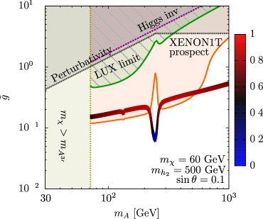
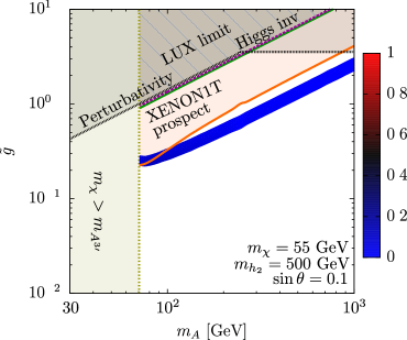
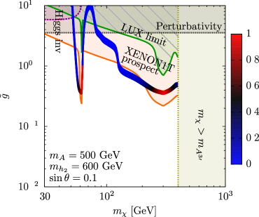
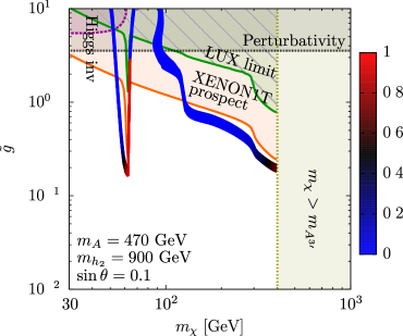
Figure 7: Dark matter constraints as in Fig. 6 for $v_{1}=1.2\,v_{2}.$

We see that the isocontours of correct relic abundance do not differ substantially from those for the case $v_{1}\gg v_{2}$.

3.2.2 Direct detection

As seen from Fig. 7, the Direct Detection limits change substantially. Even though there is a cancellation in $\sigma_{\chi N}$ as described before, for $v_{1}\sim v_{2}$ it is incomplete. The mixing term $A^{\mu\,6}\partial_{\mu}\chi$ is now important since $A^{\mu\,6}$ does not decouple. Eliminating this term by field redefinition leads to an additional coupling that scales as $m_{A^{6}}^{-2}$. The resulting $\chi$–$N$ scattering cross section is then

$$\frac{\sigma_{\chi N}}{\sigma_{AN}}\simeq\frac{m_{\chi}^{2}}{m_{A}^{2}}\left(\frac{v_{2}^{2}}{v_{1}^{2}+v_{2}^{2}}\right)^{2}\,,$$ (45)

where $\sigma_{AN}$ is given by Eq. (43). Unlike in the case $v_{1}\gg v_{2}$ (i.e. $m_{A^{6}}\gg m_{A}$), this cross section is significant. Note that $\sigma_{\chi N}$ is suppressed by the factor $m_{\chi}^{2}/m_{A}^{2}$ with respect to $\sigma_{AN}$.

In the presence of non-negligible scattering cross-sections for both DM components, the analysis of the Direct Detection limits is not straightforward. Such limits are normally given in terms of the DM–nucleon scattering cross-section as a function of the DM mass. In our case, one should compare directly the experimental outcome, i.e. the distribution of events with respect to the recoil energy, with the theoretical prediction

$$\frac{dN}{dE_{R}}=\sum_{i=\chi,A}f_{i}{\left(\frac{dN}{dE_{R}}\right)}_{i}\,.$$ (46)

Here $f_{i}=\Omega_{i}/\Omega_{\rm tot}$ and

$${\left(\frac{dN}{dE_{R}}\right)}_{i}=\frac{\sigma_{iN}\rho_{0}}{2m_{R}^{2}m_{i}}F_{i}^{2}(E_{R})\int_{v_{\mathrm{min}}(E_{R})}^{\infty}\frac{f(v_{i})}{v_{i}}dv_{i}\,,$$ (47)

with $\rho_{0}$ being the experimental value of the local DM density; $m_{R}$ is the reduced mass of the DM–nucleus system, $F_{i}(E_{R})^{2}$ is the form-factor due to the finite size of the nucleus (normalized to $F_{i}(0)^{2}=1$), and $f(v_{i})$ is the DM velocity distribution in the detector frame. A detailed discussion of the Direct Detection limit interpretation for multicomponent DM is given in [20, 19]. Here we have adopted a simple approximate procedure. We have computed the total number of recoil events, obtained by integrating the distribution of Eq. (46) over a suitable range of recoil energies and multiplied the result with the number of nuclei and the exposure time in a given experiment. Given the design similarity between the LUX and XENON1T experiments, we have assumed the upper limit of 3 events for both (with two years of exposure time) [44]. This number takes into account the detector efficiency which is set to 1 in Micromegas.

It is seen from Fig. 7 that the contribution from the pseudoscalar component tightens the limits from DD. Yet, the thermal DM relic density band is still out of reach of LUX. The relevant Direct Detection suppression factors include a low value of $\sin\theta$, $m_{\chi}^{2}/m_{A}^{2}$ for a light $\chi$ component as well as a relatively small $\tilde{g}$ in the domain of the broad resonance $m_{\chi}\sim{\cal O}(m_{h_{2}}/2)$. We find that these factors are efficient enough to make the detection of a light $\chi$ beyond the reach of XENON1T, while some regions with a heavier $\chi$ can be probed. This differs from the pure vector DM case considered in [25].

3.3 Complementarity of direct and indirect detection

In this subsection, we briefly explore the possibility of observing one DM component in Indirect Detection (ID) experiments and the other one through Direct Detection.

As seen in Eqs. (• ‣ 3.1.1,• ‣ 3.1.1), the pair annihilation cross-sections are s-wave dominated and suffer no velocity suppression. Therefore, both the pseudoscalar and the vector DM components can potentially generate an ID (photon) signal from the $\bar{b}b,\bar{t}t,W^{+}W^{-},ZZ,hh$ final states. However, as explained in the previous subsections, the vector component often annihilates into $\chi\chi$ most efficiently. As a result, the ID signal would be suppressed and thus only the pseudoscalar component could potentially be detected. This situation reverses in Direct Detection since the $\sigma_{\chi N}$ cross section is too small.

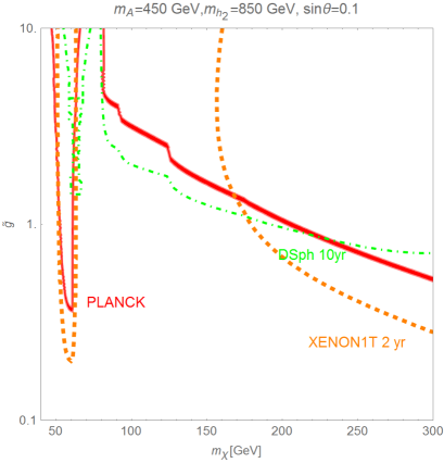
Figure 8: Prospects of detecting directly the vector DM component and indirectly the pseudoscalar DM component. The red band corresponds to the correct total DM relic density, the orange dashed line represents projected DD limits from XENON1T with a 2 year exposure time and the dashed green line shows projected ID limits from FERMI [46] with 10 years of data taking [47].

While a detailed analysis is beyond the scope of this work, we illustrate this point with the following example (Fig. 8). We take $m_{h_{2}}=850~{}{\rm GeV}$, $m_{A}=450~{}{\rm GeV}$, $s_{\theta}=0.1$ and focus on the range $50-300~{}{\rm GeV}$ for the $\chi$ mass. These parameters are chosen in order to have a large pseudoscalar component since the ID rate scales with the square of the DM density.

We see that there are two small regions in Fig. 8 where both ID and DD signals could be detected. The first one is close to the $h_{1}$ resonance, i.e. for $m_{\chi}\simeq 60~{}{\rm GeV}$. This region may in fact be compatible with the Galactic Center gamma-ray excess [48] although reproducing it in vicinity of the s-channel resonances is in general rather contrived [49]. The second region corresponds to masses $m_{\chi}\sim 170-230\,\mbox{GeV}$. In this region, the density fraction of the vectorial DM component is very low, for example, $f_{A}\approx 0.02$ at $m_{\chi}=170\,\mbox{GeV}$. This is compensated by the high DD cross section since the correct relic density requires $\tilde{g}\simeq 1$. Specifically, for $m_{A}=450\,\mbox{GeV}$ and $m_{\chi}=170\,\mbox{GeV}$, one has $f_{A}\sigma_{NA}\approx 7.5\times 10^{-47}\,{\mbox{cm}}^{2}$.

A complication here is that it is very difficult to prove that DD and ID signals come from particles with different masses. One obstacle is the large uncertainty (hundreds of GeV) in the DM mass determination through Direct Detection (cf. eg. [50]). This stems from the very weak dependence of the spectrum of recoil events on the DM mass (for heavy DM). Thus, in practice it would be challenging to prove that Dark Matter is indeed multicomponent.

Further information which can help deciphering the DM composition would be provided by collider experiments. In particular, in certain kinematic regimes, e.g. $m_{h_{2}}>2m_{A}$ and $m_{h_{2}}<300$ GeV, the LHC monojet events with missing energy will be able to probe the hidden sector gauge coupling in the range ${\cal O}(10^{-1})-{\cal O}(1)$ [51]. Similar constraints are obtained in Vector Boson Fusion [52] (see also [53]). Other channels can provide further probes, which will be studied elsewhere.

4 Conclusions

We have studied a simple UV complete set–up which entails naturally multicomponent Dark Matter with spin-1 and spin-0 constituents. The symmetry that stabilizes DM is not put in by hand, but is instead inherent in the Yang–Mills system. The model belongs to the Higgs portal category with the hidden sector consisting of SU(3) Yang–Mills fields as well as the minimal Higgs content to break this symmetry completely. Upon spontaneous gauge symmetry breaking, the system retains a global $U(1)\times Z_{2}^{\prime}$ symmetry (assuming unbroken CP in the hidden sector). We focus on its discrete subgroup $Z_{2}\times Z_{2}^{\prime}$ which can be regarded as a DM stabilizer making the lightest vector fields and a pseudoscalar stable. These play the role of multicomponent Dark Matter.

Even though the theory is rather simple in the UV, the DM phenomenology is very rich offering a number of qualitatively different parametric regimes. For instance, the “dark annihilation” channel, where the heavier DM component pair–annihilates into the lighter component, can play an important role. Dark Matter can be mostly spin-1, mostly spin-0 or mixed. An attractive feature of the model is that the Direct DM Detection rate is suppressed as long as the SM Higgs mixes predominantly with a single scalar of the hidden sector. This phenomenon is qualitatively different from the known DD suppression mechanisms. We find that in many regions of parameter space, the Direct Detection rate is well below the LUX2016 (and sometimes XENON1T) constraint while still consistent with the thermal WIMP paradigm.

This shows, in particular, that the Higgs portal Dark Matter framework offers a number of viable options and the WIMP paradigm is not necessarily in crisis.

Acknowledgements

The authors thank A. Pukhov for his help with the package Micromegas. G.A. acknowledges support from the ERC advanced grant Higgs@LHC. C.G. is grateful to the Mainz Institute for Theoretical Physics (MITP), where a part of this work was done, for its hospitality and partial financial support. C.G. and O.L. acknowledge support from the Academy of Finland, project The Higgs Boson and the Cosmos. This project has received funding from the European Union’s Horizon 2020 research and innovation programme under the Marie Sklodowska-Curie grant agreement No 674896. S.P. is supported by the National Science Centre, Poland, under research grants DEC-2014/15/B/ST2/02157, DEC-2015/19/B/ST2/02848 and DEC-2015/18/M/ST2/00054. T.T. acknowledges support from P2IO Excellence Laboratory (LABEX).

References

- [1] P. A. R. Ade et al. [Planck Collaboration], arXiv:1303.5076 [astro-ph.CO].
- [2] V. Silveira and A. Zee, Phys. Lett. 161B, 136 (1985).
- [3] B. Patt and F. Wilczek, hep-ph/0605188.
- [4] J. March-Russell, S. M. West, D. Cumberbatch and D. Hooper, JHEP 0807 (2008) 058 [arXiv:0801.3440 [hep-ph]].
- [5] S. Andreas, T. Hambye and M. H. G. Tytgat, JCAP 0810 (2008) 034 [arXiv:0808.0255 [hep-ph]].
- [6] T. Hambye, JHEP 0901, 028 (2009) [arXiv:0811.0172 [hep-ph]].
- [7] S. Kanemura, S. Matsumoto, T. Nabeshima and N. Okada, Phys. Rev. D 82 (2010) 055026 [arXiv:1005.5651 [hep-ph]].
- [8] O. Lebedev, H. M. Lee and Y. Mambrini, Phys. Lett. B 707 (2012) 570 [arXiv:1111.4482 [hep-ph]].
- [9] A. Djouadi, O. Lebedev, Y. Mambrini and J. Quevillon, Phys. Lett. B 709, 65 (2012) [arXiv:1112.3299 [hep-ph]].
- [10] Y. G. Kim and K. Y. Lee, Phys. Rev. D 75 (2007) 115012 [hep-ph/0611069].
- [11] L. Lopez-Honorez, T. Schwetz and J. Zupan, Phys. Lett. B 716 (2012) 179 [arXiv:1203.2064 [hep-ph]].
- [12] Y. Farzan and A. R. Akbarieh, JCAP 1210 (2012) 026 [arXiv:1207.4272 [hep-ph]].
- [13] S. Baek, P. Ko, W. I. Park and E. Senaha, JHEP 1305, 036 (2013) [arXiv:1212.2131 [hep-ph]].
- [14] M. Duch, B. Grzadkowski and M. McGarrie, JHEP 1509, 162 (2015) [arXiv:1506.08805 [hep-ph]].
- [15] D. S. Akerib et al. [LUX Collaboration], arXiv:1310.8214 [astro-ph.CO]; D. S. Akerib et al. [LUX Collaboration], arXiv:1512.03506 [astro-ph.CO].
- [16] A. Tan et al. [PandaX-II Collaboration], Phys. Rev. Lett. 117, no. 12, 121303 (2016) [arXiv:1607.07400 [hep-ex]].
- [17] G. Belanger and J. C. Park, JCAP 1203 (2012) 038 doi:10.1088/1475-7516/2012/03/038 [arXiv:1112.4491 [hep-ph]].
- [18] E. Dudas, L. Heurtier and Y. Mambrini, Phys. Rev. D 90 (2014) 035002 [arXiv:1404.1927 [hep-ph]].
- [19] K. R. Dienes, J. Kumar and B. Thomas, Phys. Rev. D 86 (2012) 055016 [arXiv:1208.0336 [hep-ph]].
- [20] S. Profumo, K. Sigurdson and L. Ubaldi, JCAP 0912 (2009) 016 [arXiv:0907.4374 [hep-ph]].
- [21] S. Esch, M. Klasen and C. E. Yaguna, JHEP 1409 (2014) 108 [arXiv:1406.0617 [hep-ph]].
- [22] K. K. Boddy, J. L. Feng, M. Kaplinghat and T. M. P. Tait, Phys. Rev. D 89, no. 11, 115017 (2014) [arXiv:1402.3629 [hep-ph]].
- [23] M. Klasen, F. Lyonnet and F. S. Queiroz, arXiv:1607.06468 [hep-ph].
- [24] A. DiFranzo and G. Mohlabeng, arXiv:1610.07606 [hep-ph].
- [25] C. Gross, O. Lebedev and Y. Mambrini, JHEP 1508 (2015) 158 [arXiv:1505.07480 [hep-ph]].
- [26] A. Karam and K. Tamvakis, Phys. Rev. D 92, no. 7, 075010 (2015) [arXiv:1508.03031 [hep-ph]].
- [27] V. V. Khoze and A. D. Plascencia, arXiv:1605.06834 [hep-ph].
- [28] A. Karam and K. Tamvakis, arXiv:1607.01001 [hep-ph].
- [29] K. J. Bae, H. Baer, A. Lessa and H. Serce, Front. in Phys. 3 (2015) 49 [arXiv:1502.07198 [hep-ph]].
- [30] M. Badziak, A. Delgado, M. Olechowski, S. Pokorski and K. Sakurai, JHEP 1511 (2015) 053 [arXiv:1506.07177 [hep-ph]].
- [31] E. Aprile et al. [XENON Collaboration], JCAP 1604 (2016) no.04, 027 [arXiv:1512.07501 [physics.ins-det]].
- [32] A. Falkowski, C. Gross and O. Lebedev, JHEP 1505 (2015) 057 [arXiv:1502.01361 [hep-ph]].
- [33] M. Aoki, M. Duerr, J. Kubo and H. Takano, Phys. Rev. D 86 (2012) 076015 [arXiv:1207.3318 [hep-ph]].
- [34] F. D’Eramo and J. Thaler, JHEP 1006 (2010) 109 [arXiv:1003.5912 [hep-ph]].
- [35] G. Belanger, K. Kannike, A. Pukhov and M. Raidal, JCAP 1204 (2012) 010 [arXiv:1202.2962 [hep-ph]].
- [36] J. Edsjo and P. Gondolo, Phys. Rev. D 56 (1997) 1879 [hep-ph/9704361].
- [37] P. Gondolo and G. Gelmini, Nucl. Phys. B 360 (1991) 145.
- [38] G. Jungman, M. Kamionkowski and K. Griest, Phys. Rept. 267 (1996) 195 [hep-ph/9506380].
- [39] G. Belanger, F. Boudjema, A. Pukhov and A. Semenov, Comput. Phys. Commun. 192, 322 (2015) [arXiv:1407.6129 [hep-ph]].
- [40] D. S. Akerib et al. [LUX Collaboration], Phys. Rev. Lett. 116 (2016) no.16, 161301 [arXiv:1512.03506 [astro-ph.CO]].
- [41] C. Boehm, M. J. Dolan, C. McCabe, M. Spannowsky and C. J. Wallace, JCAP 1405 (2014) 009 [arXiv:1401.6458 [hep-ph]].
- [42] O. Lebedev and Y. Mambrini, Phys. Lett. B 734, 350 (2014) [arXiv:1403.4837 [hep-ph]].
- [43] A. Crivellin, M. Hoferichter and M. Procura, Phys. Rev. D 89 (2014) 054021 [arXiv:1312.4951 [hep-ph]].
- [44] C. Savage, A. Scaffidi, M. White and A. G. Williams, Phys. Rev. D 92 (2015) no.10, 103519 [arXiv:1502.02667 [hep-ph]].
- [45] Y. Akrami, C. Savage, P. Scott, J. Conrad and J. Edsjo, JCAP 1104 (2011) 012 [arXiv:1011.4318 [astro-ph.CO]].
- [46] M. Ackermann et al. [Fermi-LAT Collaboration], Phys. Rev. D 89 (2014) 4, 042001 [arXiv:1310.0828 [astro-ph.HE]].
- [47] Private communication from German Gomez.
- [48] D. Hooper and L. Goodenough, Phys. Lett. B 697 (2011) 412 [arXiv:1010.2752 [hep-ph]]; D. Hooper and T. Linden, Phys. Rev. D 84 (2011) 123005 [arXiv:1110.0006 [astro-ph.HE]]; K. N. Abazajian and M. Kaplinghat, Phys. Rev. D 86 (2012) 083511 [arXiv:1207.6047 [astro-ph.HE]]; C. Gordon and O. Macias, Phys. Rev. D 88 (2013) 083521 [arXiv:1306.5725 [astro-ph.HE]]. K. N. Abazajian, N. Canac, S. Horiuchi and M. Kaplinghat, Phys. Rev. D 90 (2014) 023526 [arXiv:1402.4090 [astro-ph.HE]]; F. Calore, I. Cholis and C. Weniger, arXiv:1409.0042 [astro-ph.CO].
- [49] C. Cheung, M. Papucci, D. Sanford, N. R. Shah and K. M. Zurek, Phys. Rev. D 90 (2014) 075011 [arXiv:1406.6372 [hep-ph]].
- [50] C. Strege, R. Trotta, G. Bertone, A. H. G. Peter and P. Scott, Phys. Rev. D 86 (2012) 023507 [arXiv:1201.3631 [hep-ph]].
- [51] J. S. Kim, O. Lebedev and D. Schmeier, JHEP 1511, 128 (2015) [arXiv:1507.08673 [hep-ph]].
- [52] C. H. Chen and T. Nomura, Phys. Rev. D 93, no. 7, 074019 (2016) [arXiv:1507.00886 [hep-ph]].
- [53] A. DiFranzo, P. J. Fox and T. M. P. Tait, JHEP 1604, 135 (2016) [arXiv:1512.06853 [hep-ph]].