Essentially high-order compact schemes with application to stochastic volatility models on non-uniform grids

Abstract

We present high-order compact schemes for a linear second-order parabolic partial differential equation (PDE) with mixed second-order derivative terms in two spatial dimensions. The schemes are applied to option pricing PDE for a family of stochastic volatility models. We use a non-uniform grid with more grid-points around the strike price. The schemes are fourth-order accurate in space and second-order accurate in time for vanishing correlation. In our numerical convergence study we achieve fourth-order accuracy also for non-zero correlation. A combination of Crank-Nicolson and BDF-4 discretisation is applied in time. Numerical examples confirm that a standard, second-order finite difference scheme is significantly outperformed.

1 Introduction

We consider the following parabolic partial differential equation for
$u~{}=~{}u(x_{1},x_{2},t)$ in two spatial dimensions and time,

$$du_{\tau}+a_{1}u_{x_{1}x_{1}}+a_{2}u_{x_{2}x_{2}}+b_{12}u_{x_{1}x_{2}}+c_{1}u_{x_{1}}+c_{2}u_{x_{2}}=0\quad\text{in }\Omega\times]0,T]=:Q_{T},$$ (1)

subject to suitable boundary conditions and initial condition $u(x_{1},x_{2},0)=u_{0}(x_{1},x_{2})$ with $T>0$ and $\Omega=\bigl{[}x_{\min}^{(1)},x_{\max}^{(1)}\bigr{]}\times\bigl{[}x_{\min}^{(2)},x_{\max}^{(2)}\bigr{]}\subset\mathbb{R}^{2}$ with $x_{\min}^{(i)}<x_{\max}^{(i)}$ for $i=1,2$. The functions $a_{i}=a_{i}(x_{1},x_{2},\tau)<0$, $b_{12}=b_{12}(x_{1},x_{2},\tau)$, $c_{i}=c(x_{1},x_{2},\tau)$, $d=d(x_{1},x_{2},\tau)$ map $Q_{T}$ to $\mathbb{R}$, and $a_{i}\left(\cdot,\tau\right)$, $b\left(\cdot,\tau\right)$, $c_{i}\left(\cdot,\tau\right)$, and $d\left(\cdot,\tau\right)$ are assumed to be in $C^{2}(\Omega)$ and $u\left(\cdot,t\right)\in C^{6}(\Omega)$ for all $\tau\in]0,T]$. We define a uniform spatial grid $G$ with step size $\Delta x_{k}$ in $x_{k}$ direction for $k=1,2$. Setting $f=-du_{\tau}$ and applying a standard, second-order central difference approximation leads to the elliptic problem

$$f= A_{0}-\frac{a_{1}(\Delta x_{1})^{2}}{12}\frac{\partial^{4}u}{\partial x_{1}^{4}}-\frac{a_{2}(\Delta x_{2})^{2}}{12}\frac{\partial^{4}u}{\partial x_{2}^{4}}-\frac{b_{12}(\Delta x_{1})^{2}}{6}\frac{\partial^{4}u}{\partial x_{1}^{3}\partial x_{2}}$$

$$-\frac{b_{12}(\Delta x_{2})^{2}}{6}\frac{\partial^{4}u}{\partial x_{1}\partial x_{2}^{3}}-\frac{c_{1}(\Delta x_{1})^{2}}{6}\frac{\partial^{3}u}{\partial x_{1}^{3}}-\frac{c_{2}(\Delta x_{2})^{2}}{6}\frac{\partial^{3}u}{\partial x_{2}^{3}}+\varepsilon,$$ (2)

with $A_{0}:=a_{1}D^{c}_{1}D^{c}_{1}U_{i_{1},i_{2}}+a_{2}D^{c}_{2}D^{c}_{2}U_{i_{1},i_{2}}+b_{12}D^{c}_{1}D^{c}_{2}U_{i_{1},i_{2}}+c_{1}D^{c}_{1}U_{i_{1},i_{2}}+c_{2}D^{c}_{2}U_{i_{1},i_{2}}$, where $D_{k}^{c}$ denotes the central difference operator in $x_{k}$ direction, and $\varepsilon\in\mathcal{O}\left(h^{4}\right)$ if $\Delta x_{k}\in\mathcal{O}\left(h\right)$ for $h>0$. We call a finite difference scheme high-order compact (HOC) if its consistency error is of order $\mathcal{O}\left(h^{4}\right)$ for $\Delta x_{1},\Delta x_{2}\in\mathcal{O}\left(h\right)$ for $h>0$, and it uses only points on the compact stencil, $U_{k,p}$ with $k\in\{i_{1}-1,i_{1},i_{1}+1\}$ and $p\in\{i_{2}-1,i_{2},i_{2}+1\}$, to approximate the solution at $\left(x_{i_{1}},x_{i_{2}}\right)\in\overset{\smash{\raisebox{-0.21529pt}{$\scriptstyle\circ$}}}{G}\rule{0.0pt}{8.61108pt}$.

2 Auxiliary relations for higher derivatives

Our aim is to replace the third- and fourth-order derivatives in (1) which are multiplied by second-order terms by equivalent expressions which can be approximated with second order on the compact stencil. Indeed, if we differentiate (1) (using $f=-du_{\tau}$) once with respect to $x_{k}$ ($k=1,2$), we obtain relations

$$\frac{\partial^{3}u}{\partial x_{1}^{3}}= A_{1},\qquad\frac{\partial^{3}u}{\partial x_{2}^{3}}=A_{2},$$ (3)

where we can discretise $A_{i}$ with second order on the compact stencil using the central difference operator. Analogously, we obtain

$$\frac{\partial^{4}u}{\partial x_{1}^{4}}= B_{1}-\frac{b_{12}}{a_{1}}\frac{\partial^{4}u}{\partial x_{1}^{3}\partial x_{2}} \iff\qquad\frac{\partial^{4}u}{\partial x_{1}^{3}\partial x_{2}} =\frac{a_{1}}{b_{12}}B_{1}-\frac{a_{1}}{b_{12}}\frac{\partial^{4}u}{\partial x_{1}^{4}},$$

$$\frac{\partial^{4}u}{\partial x_{2}^{4}}= B_{2}-\frac{b_{12}}{a_{2}}\frac{\partial^{4}u}{\partial x_{1}\partial x_{2}^{3}} \iff\qquad\frac{\partial^{4}u}{\partial x_{1}\partial x_{2}^{3}} =\frac{a_{2}}{b_{12}}B_{2}-\frac{a_{2}}{b_{12}}\frac{\partial^{4}u}{\partial x_{2}^{4}},$$ (4)

$$\frac{\partial^{4}u}{\partial x_{1}^{3}\partial x_{2}}= C_{1}-\frac{a_{2}}{a_{1}}\frac{\partial^{4}u}{\partial x_{1}\partial x_{2}^{3}} \iff\qquad\frac{\partial^{4}u}{\partial x_{1}\partial x_{2}^{3}} =C_{2}-\frac{a_{1}}{a_{2}}\frac{\partial^{4}u}{\partial x_{1}^{3}\partial x_{2}},$$

where we can approximate $B_{k}$ and $C_{k}$ with second order on the compact stencil using the central difference operator. A detailed derivation can be found in [3, 5].

3 Derivation of high-order compact schemes

In general it is not possible to obtain a HOC scheme for (1), since there are four fourth-order derivatives in (1), but only three auxiliary equations for these in (2). Hence, we propose four different versions of the numerical schemes, where only one of the fourth-order derivatives in (1) is left as a second-order remainder term. Using (3) and (2) in (1) we obtain as Version 1 scheme

$$\begin{split}f=&A_{0}-\frac{c_{1}(\Delta x_{1})^{2}}{6}A_{1}-\frac{c_{2}(\Delta x_{2})^{2}}{6}A_{2}-\frac{a_{2}(\Delta x_{2})^{2}}{12}B_{2}-\frac{b_{12}(\Delta x_{2})^{2}}{12}C_{2}\\ &-\frac{a_{1}\left(2a_{2}(\Delta x_{1})^{2}-a_{1}(\Delta x_{2})^{2}\right)}{12a_{2}}B_{1}+\frac{a_{1}\left(a_{2}(\Delta x_{1})^{2}-a_{1}(\Delta x_{2})^{2}\right)}{12a_{2}}\frac{\partial^{4}u}{\partial x_{1}^{4}}+\varepsilon,\end{split}$$ (5)

as Version 2 scheme

$$\begin{split}f=&A_{0}-\frac{c_{1}(\Delta x_{1})^{2}}{6}A_{1}-\frac{c_{2}(\Delta x_{2})^{2}}{6}A_{2}-\frac{a_{1}(\Delta x_{1})^{2}}{12}B_{1}-\frac{b_{12}(\Delta x_{1})^{2}}{12}C_{1}\\ &-\frac{a_{2}\left(2a_{1}(\Delta x_{2})^{2}-a_{2}(\Delta x_{1})^{2}\right)}{12a_{1}}B_{2}+\frac{a_{2}\left(a_{1}(\Delta x_{2})^{2}-a_{2}(\Delta x_{1})^{2}\right)}{12a_{1}}\frac{\partial^{4}u}{\partial x_{2}^{4}}+\varepsilon,\end{split}$$ (6)

as Version 3 scheme

$$\begin{split}f=&A_{0}-\frac{c_{1}(\Delta x_{1})^{2}}{6}A_{1}-\frac{c_{2}(\Delta x_{2})^{2}}{6}A_{2}-\frac{a_{1}(\Delta x_{1})^{2}}{12}B_{1}-\frac{a_{2}(\Delta x_{2})^{2}}{12}B_{2}\\ &-\frac{b_{12}(\Delta x_{2})^{2}}{12}C_{2}+\frac{b_{12}\left(a_{1}(\Delta x_{2})^{2}-a_{2}(\Delta x_{1})^{2}\right)}{12a_{2}}\frac{\partial^{4}u}{\partial x_{1}^{3}\partial x_{2}}+\varepsilon,\end{split}$$ (7)

and, finally, as Version 4 scheme

$$\begin{split}f=&A_{0}-\frac{c_{1}(\Delta x_{1})^{2}}{6}A_{1}-\frac{c_{2}(\Delta x_{2})^{2}}{6}A_{2}-\frac{a_{1}(\Delta x_{1})^{2}}{12}B_{1}-\frac{a_{2}(\Delta x_{2})^{2}}{12}B_{2}\\ &-\frac{b_{12}(\Delta x_{1})^{2}}{12}C_{1}+\frac{b_{12}\left(a_{2}(\Delta x_{1})^{2}-a_{1}(\Delta x_{2})^{2}\right)}{12a_{1}}\frac{\partial^{4}u}{\partial x_{1}\partial x_{2}^{3}}+\varepsilon.\end{split}$$ (8)

Employing the central difference operator with $\Delta x=\Delta y=h$ for $h>0$ to discretise $A_{i},$ $B_{i},$ $C_{i},$ in (5)–(8) and neglecting the remaining lower-order term leads to four semi-discrete (in space) schemes. A more detailed description of this approach can be found in [3, 5]. When $a_{1}\equiv a_{2}$ or $b_{12}\equiv 0$ these schemes are fourth-order consistent in space, otherwise second-order.

In time, we apply the implicit BDF4 method on an equidistant time grid with stepsize $k\in\mathcal{O}\bigl{(}h\bigr{)}$. The necessary starting values are obtained using a Crank-Nicolson time discretisation, where we subdivide the first timesteps with a step size $k^{\prime}\in\mathcal{O}\left(h^{2}\right)$ to ensure the fourth-order time discretisation in terms of $h$.

With additional information on the solution of (1) even better results are possible. If the specific combination of pre-factors in (1) and the higher derivatives in the second-order terms is sufficiently small, the second-order term dominates the computational error only for very small step-sizes $h$. Before this error term becomes dominant one can observe a fourth-order numerical convergence. In this case we call the scheme essentially high-order compact (EHOC).

4 Application to option pricing

In this section we apply our numerical schemes to an option pricing PDE in a family of stochastic volatility models, with a generalised square root process for the variance with nonlinear drift term,

$$dS_{t}= \mu S_{t}{\rm d}t+\sqrt{v_{t}}S_{t}{\rm d}W^{(1)}_{t},\qquad dv_{t}=\kappa v_{t}^{\alpha}\left(\theta-v_{t}\right){\rm d}t+\sigma\sqrt{v_{t}}{\rm d}W^{(2)}_{t},$$

with $\alpha\geq 0$, a correlated, two-dimensional Brownian motion, $dW_{t}^{(1)}dW_{t}^{(2)}=\rho dt$, as well as drift $\mu\in\mathbb{R}$ of the stock price $S$, long run mean $\theta>0$, mean reversion speed $\kappa>0$, and volatility of volatility $\sigma>0$. For $\alpha=0$ one obtains the standard Heston model, for $\alpha=1$ the SQRN model, see [1]. Using Itô’s lemma and standard arbitrage arguments, the option price $V=V(S,v,t)$ solves

$$\frac{\partial V}{\partial t}+\frac{vS^{2}}{2}\frac{\partial^{2}V}{\partial S^{2}}+\rho\sigma vS\frac{\partial^{2}V}{\partial S\partial v}+\frac{\sigma^{2}v}{2}\frac{\partial^{2}V}{\partial v^{2}}+rS\frac{\partial V}{\partial S}+\kappa v^{\alpha}\left(\theta-v\right)\frac{\partial V}{\partial v}-rV=0,$$ (9)

where $S,\sigma>0$ and $t\in\left[0,T\right[$ with $T>0$. For a European Put with exercise price $K$ we have the final condition $V(S,T)=\max\left(K-S,0\right)$. The transformations $\tau=T-t$, $u=e^{r\tau}{V}/{K},$ $\hat{S}=\ln({S}/{K}),$ $y={v}/{\sigma}$ as well as $\hat{S}=\varphi\left(x\right)$ [2], lead to

$$\varphi_{x}^{3}u_{\tau}+\frac{\sigma y}{2}\left[\varphi_{x}u_{xx}+\varphi_{x}^{3}u_{yy}\right]-\rho\sigma y\varphi_{x}^{2}u_{xy}\\ +\left[\frac{\sigma y\varphi_{xx}}{2}+\Bigl{(}\frac{\sigma y}{2}-r\Bigr{)}\varphi_{x}^{2}\right]u_{x}-\kappa\sigma^{\alpha}y^{\alpha}\frac{\theta-\sigma y}{\sigma}\varphi_{x}^{3}u_{y}=0,$$

with initial condition $u(x,y,0)=\max\left(1-e^{\varphi(x)},0\right)$. The function $\varphi$ is considered to be four times differentiable and strictly monotone. It is chosen in such a way that grid points are concentrated around the exercise price $K$ in the $S$–$v$ plane when using a uniform grid in the $x$–$y$ plane.

Dirichlet boundary conditions are imposed at $x=x_{\min}$ and $x=x_{\max}$ similarly as in [2],

$$u(x_{\min},y,\tau)=u(x_{\min},y,0),\quad u(x_{\max},y,\tau)=u(x_{\max},y,0),$$

for all $\tau\in[0,\tau_{\max}]$ and $y\in[y_{\min},y_{\max}].$ At the boundaries ${y=y_{\min}}$ and ${y=y_{\max}}$ we employ the discretisation of the interior spatial domain and extrapolate the resulting ghost-points using

$$U_{i,-1} =3U_{i,0}-3U_{i,1}+U_{i,2}+\mathcal{O}\bigl{(}h^{3}\bigr{)},$$

$$U_{i,M+1} =3U_{i,M}-3U_{i,M-1}+U_{i,M-2}+\mathcal{O}\bigl{(}h^{3}\bigr{)},$$

for $i=0,\ldots,N$. Third-order extrapolation is sufficient here to ensure overall fourth-order convergence [4].

5 Numerical experiments

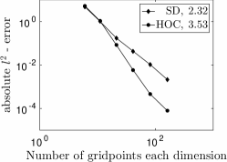
We employ the function $\varphi(x)=\sinh(c_{2}x+c_{1}(1-x))/\zeta,$ where $c_{1}=\text{asinh}(\zeta\hat{S}_{\min})$, $c_{2}=\text{asinh}(\zeta\hat{S}_{\max})$ and $\zeta>0$. We use $\kappa=1.1$, $\theta=0.2$, $v=0.3$, $r=0.05$, $K=100$, $T=0.25$, $v_{\min}=0.1$, $v_{\max}=0.3$, $S_{\min}=1.5$, $S_{\max}=250$, $\rho=0,-0.4$ and $\zeta=7.5$. Hence, $x_{\max}-x_{\min}=y_{\max}-y_{\min}=1$. For the Crank-Nicolson method we use $k^{\prime}/h^{2}=0.4$, for the BDF4 method $k/h=0.1$. We smooth the initial condition according to [6, 3], so that the smoothed initial condition tends towards the original initial condition for $h\rightarrow 0$. We neglect the case $\alpha=0$ (Heston model), since a numerical study of that case has been performed in [2]. In the numerical convergence plots we use a reference solution $U_{\text{ref}}$ on a fine grid ($h=1/320$) and report the absolute $l^{2}$-error compared to $U_{\text{ref}}$. The numerical convergence order is computed from the slope of the linear least square fit of the points in the log-log plot.

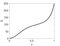
(a) Transformation with $\zeta=7.5$

(b) HOC: $\alpha=0.25$, $\rho=0$

(c) HOC: $\alpha=0.5$, $\rho=0$

(d) HOC: $\alpha=0.75$, $\rho=0$

(e) HOC: SQRN model, $\rho=0$

(f) EHOC: $\alpha=0.25$, $\rho=-0.4$

(g) EHOC: $\alpha=0.5$, $\rho=-0.4$

(h) EHOC: $\alpha=0.75$, $\rho=-0.4$

(i) EHOC: SQRN model, $\rho=-0.4$

Figure 1: Transformation of the spatial grid and numerical convergence plots.

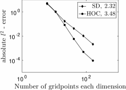
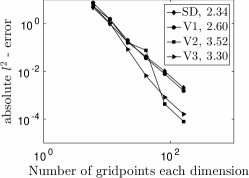
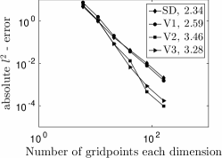
Figure 1(a) shows the transformation from $x$ to $S$. The transformation focuses on the region around the strike price. Figures 1(b), 1(c), 1(d) and 1(e) show that the HOC schemes lead to a numerical convergence order of about $3.5$, whereas the standard, second-order central difference discretisation (SD) leads to convergence orders of about $2.3$, in the case of vanishing correlation. In all cases with non-vanishing correlation ($\rho\neq 0$) we observe only slightly improved convergence for Version 1 (V1) when comparing it to the standard discretisation. Version 2 (V2) and Version 3 (V3), however, lead to similar convergence orders as the HOC scheme, even for non-vanishing correlation. Results of Version 4 are not shown as this scheme shows instable behaviour in this example.

In summary, we obtain high-order compact schemes for vanishing correlation and achieve high-order convergence also for non-vanishing correlation for the family (9) of stochastic volatility model. A standard, second-order discretisation is significantly outperformed in all cases.

Acknowledgment

BD acknowledges support by the Leverhulme Trust research project grant ‘Novel discretisations for higher-order nonlinear PDE’ (RPG-2015-69). CH was supported by the European Union in the FP7-PEOPLE-2012-ITN Program under Grant Agreement Number 304617 (FP7 Marie Curie Action, Project Multi-ITN STRIKE – Novel Methods in Computational Finance).

References

• [1] P. Christoffersen, K. Jacobs and K. Mimouni. Models for S&P500 dynamics: evidence from realized volatility, daily returns, and option prices. Rev. Financ. Stud., 23(8):3141–3189, 2010.
• [2] B. Düring, M. Fournié and C. Heuer. High-order compact finite difference schemes for option pricing in stochastic volatility models on non-uniform grids. J. Comput. Appl. Math., 271(18):247–266, 2014.
• [3] B. Düring and C. Heuer. High-order compact schemes for parabolic problems with mixed derivatives in multiple space dimensions. SIAM J. Numer. Anal., 53(5):2113–2134, 2015.
• [4] B. Gustafsson. The convergence rate for difference approximations to general mixed initial-boundary value problems. SIAM J. Numer. Anal., 18(2):179–190, 1981.
• [5] C. Heuer. High-order compact finite difference schemes for parabolic partial differential equations with mixed derivative terms and applications in computational finance. PhD thesis, University of Sussex, August 2014. http://sro.sussex.ac.uk/49800/
• [6] H.O. Kreiss, V. Thomee and O. Widlund. Smoothing of initial data and rates of convergence for parabolic difference equations. Commun. Pure Appl. Math., 23:241–259, 1970.