Open charm-bottom scalar tetraquarks and their strong decays

Abstract

The mass and meson-current coupling of the diquark-antidiquark states with the quantum numbers $J^{P}=0^{+}$ and quark contents $Z_{q}=[cq][\bar{b}\bar{q}]$ and $Z_{s}=[cs][\bar{b}\bar{s}]$ are calculated using two-point QCD sum rule approach. In calculations the quark, gluon and mixing condensates up to eight dimensions are taken into account. The parameters of the scalar tetraquarks extracted from this analysis are employed to explore the strong vertices $Z_{q}B_{c}\pi$, $Z_{q}B_{c}\eta$ and $Z_{s}B_{c}\eta$ and compute the couplings $g_{Z_{q}B_{c}\pi}$, $g_{Z_{q}B_{c}\eta}$ and $g_{Z_{s}B_{c}\eta}$. The strong couplings are obtained within the soft-meson approximation of QCD light-cone sum rule method: they form, alongside with other parameters, the basis for evaluating the widths of $Z_{q}\to B_{c}\pi$, $Z_{q}\to B_{c}\eta$ and $Z_{s}\to B_{c}\eta$ decays. Obtained in this work results for the mass of the tetraquarks $Z_{q}$ and $Z_{s}$ are compared with available predictions presented in the literature.

I Introduction

During last decade the various experimental collaborations reported on observation of hadronic states, which can not be described as the traditional hadrons composed of two or three valence quarks. Indeed, starting from the discovery of the $X(3872)$ state by the Belle Collaboration Belle:2003 (see, also Ref. D0:2004 ) measurements of various annihilation, collision and decay processes lead to valuable experimental data on the $XYZ$ family of exotic particles.

Situation with the theoretical models, computational methods and schemes proposed to explain observed features of the exotic states is more complicated. One of the essential problems here is revealing the quark-gluon structure of the exotic hadrons. Thus, in accordance with existing theoretical models the exotic hadrons are four-quark (tetraquarks), five-quark (pentaquarks) states, or contain as constituents valence gluons (hybrids, glueballs). The second question is the internal quark-gluon organization and new constituents (diquarks, antidiquarks, conventional mesons, etc.) of the exotic hadrons, as well as a nature of the forces binding them into compact states. Finally, one has to determine computational methods, which can be applied to carry out qualitative analysis these multi-quark systems. In other words, one needs to adapt to the exotic hadrons the well known methods, which were successfully used to explore conventional mesons and baryons, and/or to invent approaches to solve newly emerged problems typical for the exotic states. We have only outlined variety of problems arising when exploring the exotic hadrons. A rather detailed information on these theoretical methods and also on collected experimental data can be found in numerous review papers Refs. Swanson:2006st ; Klempt:2007cp ; Godfrey:2008nc ; Voloshin:2007dx ; Nielsen:2010 ; Faccini:2012pj ; Esposito:2014rxa ; Meyer:2015eta ; Chen:2016qju ; Lebed:2016hpi , including most recent ones Chen:2016qju ; Lebed:2016hpi , and in references therein.

Most of the observed tetraquark states belong to the class of so-called hidden charm or bottom particles containing the $c\bar{c}$ or $b\bar{b}$ pair. But, first principles of QCD do not forbid existence of the open charm (or bottom) or open charm-bottom tetraquarks. Experimental information concerning the open charm tetraquarks is restricted by the observed $D_{s0}^{\star}(2317)$ and $D_{s1}(2460)$ mesons, which are considered as candidates for such exotic states. These particles were explored both as the diquark-antidiquark states and molecules built of the conventional mesons. The only candidate to the open bottom tetraquark is $X(5568)$ state, which is also considering as the first particle containing four valence quarks of different flavors. But experimental status of this particle remains controversial and unclear. Thus, the evidence for this resonance was reported by the D0 Collaboration in Ref. D0:2016mwd , later conformed from analysis of the semileptonic decays of $B_{s}^{0}$ meson in Ref. D0 . At the same time, LHCb and CMS collaborations could not prove an existence of this state on the basis of relevant experimental data [Refs. Aaij:2016iev ; CMS:2016 ]. Numerous theoretical studies of $X(5568)$ state also suffer from contradictory conclusions ranging from conforming its parameters measured by the D0 Collaboration till explaining the observed experimental output by some alternative effects. Avoiding here further details, we refer to original works addressed various aspects of the $X(5568)$ physics, and also to the review paper devoted to the open charm and bottom mesons [Ref. Chen:2016spr ].

The open charm-bottom tetraquarks form the next class of the exotic particles. It is worth noting they have not been discovered experimentally, and to our best knowledge, there are not under consideration candidates for these states. Nevertheless, the open charm-bottom states attracted already interest of theorists, which performed their analysis within both the molecule [Refs. Zhang:2009vs ; Zhang:2009em ; Sun:2012sy ; Albuquerque:2012rq ] and diquark-antidiquark pictures [Refs. Zouzou:1986qh ; SilvestreBrac:1993ry ; Chen:2013aba ] of the tetraquark model. Thus, in Ref. Chen:2013aba the authors considered the scalar and axial-vector open charm-bottom tetraquarks and calculated their masses by means of QCD two-point sum rules. In this article some possible decay channels of these states are emphasized, as well.

In the present work we are going to study the scalar open charm-bottom exotic states $Z_{q}=[cq][\bar{b}\bar{q}]$ and $Z_{s}=[cs][\bar{b}\bar{s}]$ built of the diquarks $[cq],\,[cs]$ and antidiquarks $[\bar{b}\bar{q}],\,[\bar{b}\bar{s}]$, where $q$ is one of the light $u$ and $d$ quarks. First we calculate the masses and meson-current couplings of these still hypothetical tetraquarks. To this end, we utilize QCD two-point sum rule approach, which is one of the powerful nonperturbative methods to calculate the parameters of the hadrons Shifman:1979 . Originally proposed to find masses, decay constants, form factors of the conventional mesons and baryons, it was successfully applied to analyze also exotic tetraquark states, glueballs and hybrid $q\overline{q}g$ resonances in Refs. Shifman:1979 ; Braun:1985ah ; Braun:1988kv ; Balitsky:1982ps ; Reinders:1985 . The QCD two-point sum rule method remains among the fruitful computational tools high energy physics to investigate the exotic states.

Next, we use obtained by this way parameters of the open charm-bottom tetraquarks to explore the strong vertices $Z_{q}B_{c}\pi$, $Z_{q}B_{c}\eta$ and $Z_{s}B_{c}\eta$ and calculate the corresponding couplings $g_{Z_{q}B_{c}\pi}$, $g_{Z_{q}B_{c}\eta}$ and $g_{Z_{s}B_{c}\eta}$ necessary for evaluating the widths of $Z_{q}\rightarrow B_{c}\pi$, $Z_{q}\rightarrow B_{c}\eta$ and $Z_{s}\rightarrow B_{c}\eta$ decays. For these purposes, we employ QCD light-cone sum method and soft-meson approximation suggested and elaborated in Refs. Braun:1989 ; Ioffe:1983ju ; Braun:1995 . This method in conjunction with the soft-meson approximation was adapted for investigation of the strong vertices consisting of a tetraquark and two conventional mesons in Ref. Agaev:2016dev . Later it was applied to calculate the decay width of the $X(5568)$ resonance and its charmed partner state (see, Refs. Agaev:2016ijz ; Agaev:2016lkl ; Agaev:2016urs ). The full version of the light-cone method was employed to analyze the strong vertices containing two tetraquarks, as well as to compute the magnetic moment some of the four-quark states in Refs. Agaev:2016srl and Agamaliev:2016wtt , respectively.

The present work is organized in the following way. In Sec. II we calculate the masses and meson-current couplings of the scalar open charm-bottom tetraquarks. Here we also compare our results with predictions made in other papers. Section III is devoted to computation of the strong couplings corresponding to the vertices $Z_{q}B_{c}\pi$, $Z_{q}B_{c}\eta$ and $Z_{s}B_{c}\eta$. In this section we calculate the widths of the decay modes $Z_{q}\rightarrow B_{c}\pi$, $Z_{q}\rightarrow B_{c}\eta$ and $Z_{s}\rightarrow B_{c}\eta$. It contains also our brief conclusions. We collect the spectral densities obtained in mass sum rules in the Appendix.

II Mass and meson-current coupling

To evaluate the masses and meson-current couplings of the diquark-antidiquark $Z_{q}=[cq][\bar{b}\bar{q}]$ and $Z_{s}=[cs][\bar{b}\bar{s}]$ states we use the two-point QCD sum rules. We present explicitly expressions necessary for computing the mass and meson-current coupling in the case of the exotic $Z_{q}$ state. The similar formulas for the particle $Z_{s}$ can be obtained from a similar manner.

The scalar tetraquark state $Z_{q}=[cq][\bar{b}\bar{q}]$ can be modeled using various interpolating currents [Ref. Chen:2013aba ]. To carry out required calculations we choose the interpolating current in the form

$$J^{q}=q_{a}^{T}C\gamma_{5}c_{b}\left(\overline{q}_{a}\gamma_{5}C\overline{b}_{b}^{T}+\overline{q}_{b}\gamma_{5}C\overline{b}_{a}^{T}\right),$$ (1)

which is symmetric under exchange of the color indices $a\leftrightarrow b$. Here $C$ is the charge conjugation matrix. For simplicity, in what follows we omit the superscript in the expressions.

The correlation function for the current $J^{q}(x)$ is given as

$$\Pi(p)=i\int d^{4}xe^{ipx}\langle 0|\mathcal{T}\{J^{q}(x)J^{q{\dagger}}(0)\}|0\rangle.$$ (2)

To derive QCD sum rule expressions for mass and meson-current coupling the correlation function has to be calculated using both the physical and quark-gluon degrees of freedom.

We compute the function $\Pi^{\mathrm{Phys}}(p)$ by suggesting, that the tetraquarks under consideration are the ground states in the relevant hadronic channels. After saturating the correlation function with a complete set of the $Z_{q}$ state and performing in Eq. (2) integral over $x$ , we get the required expression for $\Pi^{\mathrm{Phys}}(p)$

$$\Pi^{\mathrm{Phys}}(p)=\frac{\langle 0|J^{q}|Z_{q}(p)\rangle\langle Z_{q}(p)|J^{q{\dagger}}|0\rangle}{m_{Z_{q}}^{2}-p^{2}}+...$$

where $m_{Z_{q}}$ is the mass of the $Z_{q}$ state, and dots stand for contributions of the higher resonances and continuum states. We define the meson-current coupling by the equality

$$\langle 0|J^{q}|Z_{q}(p)\rangle=f_{Z_{q}}m_{Z_{q}}.$$

Then in terms of $m_{Z_{q}}$ and $f_{Z_{q}}$ the correlation function takes the simple form

$$\Pi^{\mathrm{Phys}}(p)=\frac{m_{Z_{q}}^{2}f_{Z_{q}}^{2}}{m_{Z_{q}}^{2}-p^{2}}+\ldots$$ (3)

It contains only one term, which is proportional to the identity matrix, and, therefore, can be replaced by the invariant function $\Pi^{\mathrm{Phys}}(p^{2})$. The Borel transformation applied to these invariant function yields

$$\mathcal{B}_{p^{2}}\Pi^{\mathrm{Phys}}(p^{2})=m_{Z_{q}}^{2}f_{Z_{q}}^{2}e^{-m_{Z_{q}}^{2}/M^{2}}+\ldots$$ (4)

In order to obtain the function $\Pi(p)$ using the quark-gluon degrees of freedom, i.e. by employing the light and heavy propagators, we substitute the interpolating current given by Eq. (1) into Eq. (2), and contract the relevant quark fields. As a result, for $\Pi^{\mathrm{QCD}}(p)$ we get:

$$\Pi^{\mathrm{QCD}}(p)=i\int d^{4}xe^{ipx}\left\{\mathrm{Tr}\left[\gamma_{5}\widetilde{S}_{b}^{b^{\prime}b}(-x)\gamma_{5}S_{q}^{aa^{\prime}}(-x)\right]\right.$$

$$\times\mathrm{Tr}\left[\gamma_{5}\widetilde{S}_{q}^{aa^{\prime}}(x)\gamma_{5}S_{c}^{bb^{\prime}}(x)\right]+\mathrm{Tr}\left[\gamma_{5}\widetilde{S}_{b}^{a^{\prime}b}(-x)\right.$$

$$\times\left.\gamma_{5}S_{q}^{b^{\prime}a}(-x)\right]\mathrm{Tr}\left[\gamma_{5}\widetilde{S}_{q}^{aa^{\prime}}(x)\gamma_{5}S_{c}^{bb^{\prime}}(x)\right]$$

$$+\mathrm{Tr}\left[\gamma_{5}\widetilde{S}_{b}^{b^{\prime}a}(-x)\gamma_{5}S_{q}^{a^{\prime}b}(-x)\right]\mathrm{Tr}\left[\gamma_{5}\widetilde{S}_{q}^{aa^{\prime}}(x)\gamma_{5}S_{c}^{bb^{\prime}}(x)\right]$$

$$\left.+\mathrm{Tr}\left[\gamma_{5}\widetilde{S}_{b}^{a^{\prime}a}(-x)\gamma_{5}S_{q}^{b^{\prime}b}(-x)\right]\mathrm{Tr}\left[\gamma_{5}\widetilde{S}_{q}^{aa^{\prime}}(x)\gamma_{5}S_{c}^{bb^{\prime}}(x)\right]\right\},$$

where we employ the notation

$$\widetilde{S}_{q(b)}^{ab}(x)=CS_{q(b)}^{Tab}(x)C,$$ (6)

with $S_{q}(x)$ and $S_{b}(x)$ being the $q$- and $b$-quark propagators, respectively.

We continue by invoking into analysis the well known expressions of the light and heavy quark propagators. For our purposes it is convenient to use the $x$-space expression of the light quark propagators, whereas for the heavy quarks we utilize their propagators given in the momentum space. Thus, for the light quarks we have:

$$S_{q}^{ab}(x)=i\delta_{ab}\frac{\not{x}}{2\pi^{2}x^{4}}-\delta_{ab}\frac{m_{q}}{4\pi^{2}x^{2}}-\delta_{ab}\frac{\langle\overline{q}q\rangle}{12}$$

$$+i\delta_{ab}\frac{\not{x}m_{q}\langle\overline{q}q\rangle}{48}-\delta_{ab}\frac{x^{2}}{192}\langle\overline{q}g\sigma Gq\rangle+i\delta_{ab}\frac{x^{2}\not{x}m_{q}}{1152}\langle\overline{q}g\sigma Gq\rangle$$

$$-i\frac{gG_{ab}^{\alpha\beta}}{32\pi^{2}x^{2}}\left[\not{x}{\sigma_{\alpha\beta}+\sigma_{\alpha\beta}}\not{x}\right]-i\delta_{ab}\frac{x^{2}\not{x}g^{2}\langle\overline{q}q\rangle^{2}}{7776}$$

$$-\delta_{ab}\frac{x^{4}\langle\overline{q}q\rangle\langle g^{2}G^{2}\rangle}{27648}+\ldots$$ (7)

For the heavy $Q=b,\ c$ quark propagator $S_{Q}^{ab}(x)$ we utilize the expression from Ref. Reinders:1984sr .

$$S_{Q}^{ab}(x)=i\int\frac{d^{4}k}{(2\pi)^{4}}e^{-ikx}\Bigg{\{}\frac{\delta_{ab}\left({\not{k}}+m_{Q}\right)}{k^{2}-m_{Q}^{2}}$$

$$-\frac{gG_{ab}^{\alpha\beta}}{4}\frac{\sigma_{\alpha\beta}\left({\not{k}}+m_{Q}\right)+\left({\not{k}}+m_{Q}\right)\sigma_{\alpha\beta}}{(k^{2}-m_{Q}^{2})^{2}}$$

$$+\frac{g^{2}G^{2}}{12}\delta_{ab}m_{Q}\frac{k^{2}+m_{Q}{\not{k}}}{(k^{2}-m_{Q}^{2})^{4}}+\frac{g^{3}G^{3}}{48}\delta_{ab}\frac{\left({\not{k}}+m_{Q}\right)}{(k^{2}-m_{Q}^{2})^{6}}$$

$$\times\left[{\not{k}}\left(k^{2}-3m_{Q}^{2}\right)+2m_{Q}\left(2k^{2}-m_{Q}^{2}\right)\right]\left({\not{k}}+m_{Q}\right)+\ldots\Bigg{\}}.$$

In Eqs. (7) and (LABEL:eq:Qprop) the standard notations

$$G_{ab}^{\alpha\beta}=G_{A}^{\alpha\beta}t_{ab}^{A},\,\,~{}~{}G^{2}=G_{\alpha\beta}^{A}G_{\alpha\beta}^{A},$$

$$G^{3}=\,\,f^{ABC}G_{\mu\nu}^{A}G_{\nu\delta}^{B}G_{\delta\mu}^{C},$$ (9)

are introduced. Here $a,\,b=1,2,3$ and $A,B,C=1,\,2\,\ldots 8$ are the color indices, and $t^{A}=\lambda^{A}/2$ with $\lambda^{A}$ being the Gell-Mann matrices. In the nonperturbative terms the gluon field strength tensor $G_{\alpha\beta}^{A}\equiv G_{\alpha\beta}^{A}(0)$ is fixed at $x=0.$

Parameters	Values
$m_{B_{c}}$	$(6275.1\pm 1.0)~{}\mathrm{MeV}$
$f_{B_{c}}$	$(528\pm 19)~{}\mathrm{MeV}$
$m_{\eta}$	$(547.862\pm 0.017)~{}\mathrm{MeV}$
$m_{\pi}$	$(134.9766\pm 0.0006)~{}\mathrm{MeV}$
$f_{\pi}$	$0.131~{}\mathrm{GeV}$
$m_{b}$	$4.18^{+0.04}_{-0.03}~{}\mathrm{GeV}$
$m_{c}$	$(1.27\pm 0.03)~{}\mathrm{GeV}$
$m_{s}$	$96^{+8}_{-4}~{}\mathrm{MeV}$
$\langle\bar{q}q\rangle$	$(-0.24\pm 0.01)^{3}$ $\mathrm{GeV}^{3}$
$\langle\bar{s}s\rangle$	$0.8\ \langle\bar{q}q\rangle$
$m_{0}^{2}$	$(0.8\pm 0.1)$ $\mathrm{GeV}^{2}$
$\langle\overline{q}g\sigma Gq\rangle$	$m_{0}^{2}\langle\bar{q}q\rangle$
$\langle\overline{s}g\sigma Gs\rangle$	$m_{0}^{2}\langle\bar{s}s\rangle$
$\langle\frac{\alpha_{s}G^{2}}{\pi}\rangle$	$(0.012\pm 0.004)$ $~{}\mathrm{GeV}^{4}$
$\langle g^{3}G^{3}\rangle$	$(0.57\pm 0.29)$ $~{}\mathrm{GeV}^{6}$

Table 1: Input parameters.

Strictly speaking, the QCD sum rule expressions are derived after fixing the same Lorentz structures in the both physical and theoretical expressions of the correlation function. In the case of the scalar particles, as we have just noted, the only Lorentz structure in these expressions is $\sim\mathrm{I}$. Hence, there is only one invariant function $\Pi^{\mathrm{QCD}}(p^{2})$ in theoretical side of the sum rule, which can be represented as the dispersion integral

$$\Pi^{\mathrm{QCD}}(p^{2})=\int_{\mathcal{M}^{2}}^{\infty}\frac{\rho^{\mathrm{QCD}}(s)ds}{s-p^{2}}+...,$$ (10)

where $\mathcal{M}=m_{b}+m_{c}+2m_{q}$, and $\rho^{\mathrm{QCD}}(s)$ is the corresponding spectral density.

The spectral density $\rho^{\mathrm{QCD}}(s)$ is the key ingredient of the sum rule calculations. The technical methods for calculation of the spectral density in the case of the tetraquark states are well known and presented in rather clear form, for example, in Refs. Agaev:2016dev ; Agaev:2016mjb . Therefore, here we omit details of calculations and move the final explicit expressions obtained for $\rho^{\mathrm{QCD}}(s)$ corresponding to $Z_{q}$ state to the Appendix. Let us note only that the spectral density is computed by taking into account condensates up to dimension eight: it depends on the quark, gluon $\langle\overline{q}q\rangle$, $\langle g^{2}G^{2}\rangle$, $\langle g^{3}G^{3}\rangle$ and mixed $\langle\overline{q}g\sigma Gq\rangle$ condensates, and ones due to their products.

Applying the Borel transformation on the variable $p^{2}$ to the invariant function $\Pi^{\mathrm{QCD}}(p^{2})$, equating the obtained expression with $\mathcal{B}_{p^{2}}\Pi^{\mathrm{Phys}}(p)$, and subtracting the contribution arising from higher resonances and continuum states, we find the final sum rules. Thus, the sum rule for the mass of the $Z_{q}$ state reads

$$m_{Z_{q}}^{2}=\frac{\int_{\mathcal{M}^{2}}^{s_{0}}ds\rho^{\mathrm{QCD}}(s)se^{-s/M^{2}}}{\int_{\mathcal{M}^{2}}^{s_{0}}ds\rho^{\mathrm{QCD}}(s)e^{-s/M^{2}}}.$$ (11)

The meson-current coupling $f_{Z_{q}}$ is given by the sum rule:

$$f_{Z_{q}}^{2}m_{Z_{q}}^{2}e^{-m_{Z_{q}}^{2}/M^{2}}=\int_{\mathcal{M}^{2}}^{s_{0}}ds\rho^{\mathrm{QCD}}(s)e^{-s/M^{2}}.$$ (12)

In Eqs. (11) and (12) by $s_{0}$ we denote the threshold parameter, that dissects the contribution of the ground state from one due to the higher resonances and continuum. Here we should remark that in the present work we calculate the meson-current couplings $f_{Z_{q}}$ and $f_{Z_{s}}$ for the first time: they are main input parameters for calculation of the strong coupling constants considered in the next section and were not analyzed in Ref.  Chen:2013aba .

The sum rules contain parameters numerical values of which should be specified. We collect the required information in Table 1. For the vacuum expectation value of the gluon field $\sim g^{3}G^{3}$ we employ the result reported in Ref. Narison:2015nxh . The remaining quark and gluon condensates are well known, and we utilize their standard values. The Table 1 contains also $B_{c}$, $\eta$ and $\pi$ meson masses and decay constants, which will serve as input parameters for computing of the strong couplings and decay widths in the next section (see, Ref. Olive:2016xmw ).

The QCD sum rules depend on the continuum threshold $s_{0}$ and Borel variable $M^{2}$. To extract reliable information from the sum rules we have to choose such regions for $s_{0}$ and $M^{2}$, where the physical quantities under question demonstrate minimal sensitivity on them. It is worth emphasizing, that namely these two parameters are the main sources of uncertainties in QCD sum rule predictions.

According to the method used, the window for the Borel parameter has to provide the convergence of the series of operator product expansion (OPE), and suppression of the higher resonance and continuum contributions to the sum rule. The convergence of OPE, i.e., the exceeding of the perturbative part to the nonperturbative contributions and reducing the contribution with increasing the dimension of the nonperturbative operators are easily achieved for the exotic states like the standard hadrons. However, in the exotic channels the pole contribution to the mass sum rules remains mainly under $50\%$ of the total integral. But, as we will see in the next section, in the case of strong couplings of the exotic states with conventional hadrons the pole contribution exceeds $70\%$ of the whole result. To find the lower boundary for $M^{2}$ we demand convergence of the OPE and exceeding of the perturbative part over the nonperturbative contribution. The upper limit for this parameter is extracted by requiring largest possible pole contribution. As a result, for $M^{2}$, in the mass and meson-current calculations, we fix the following range

$$6.5\ \mathrm{GeV}^{2}\leq M^{2}\leq 7.5\ \mathrm{GeV}^{2}.$$ (13)

The choice of the continuum threshold $s_{0}$ depends on the energy of the first excited state and can be extracted from analysis of the pole/total ratio. This criterium enables us to determine the range of $s_{0}$ as

$$55\ \mathrm{GeV}^{2}\leq s_{0}\leq 57\ \mathrm{GeV}^{2}.$$ (14)

To see how the OPE converges and how large is the pole contribution some plots are in order. We compare the perturbative and nonperturbative contributions to the mass sum rule by varying $M^{2}$ at fixed average value of $s_{0}$, and by varying $s_{0}$ at fixed average $M^{2}$ in the left and right panels of Fig. 1, respectively. The contributions of different nonperturbative operators with respect to $M^{2}$ at average value of the continuum threshold and the same quantity with respect to $s_{0}$ at average value of $M^{2}$ are presented in the left and right panels of Fig. 2, respectively. The pole/total contribution that is shown by PC also on $M^{2}$ and $s_{0}$ are depicted in Fig. 3.

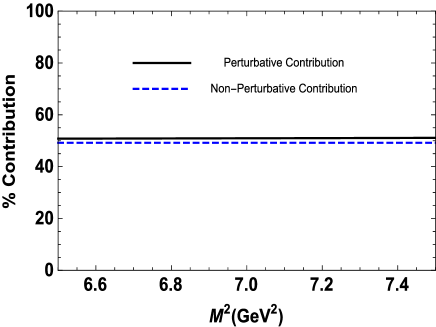
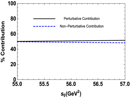
Figure 1: Left: Comparison of the perturbative and nonperturbative contributions to the mass sum rule of $Z_{q}$ with respect to $M^{2}$ at average value of $s_{0}$. Right: The same as left panel but in terms of $s_{0}$ at average value of the Borel parameter $M^{2}$.

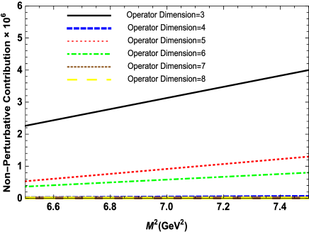
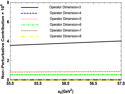
Figure 2: Left: Contribution of different nonperturbative operators to the mass sum rule of $Z_{q}$ with respect to $M^{2}$ at average value of $s_{0}$. Right: The same as left panel but in terms of $s_{0}$ at average value of the Borel parameter $M^{2}$.

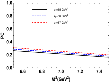
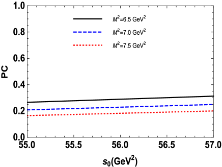
Figure 3: Left: Pole/total contribution for mass sum rule of $Z_{q}$ with respect to $M^{2}$ at different fixed values of $s_{0}$. Right: The same as left panel but in terms of $s_{0}$ at different fixed values of the Borel parameter $M^{2}$.

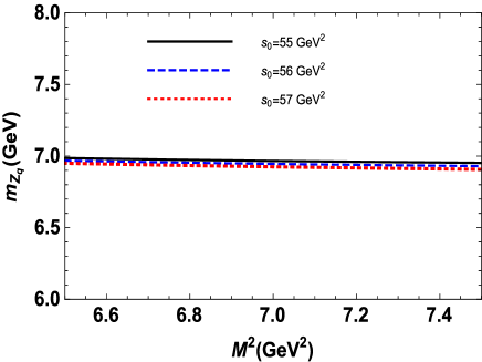
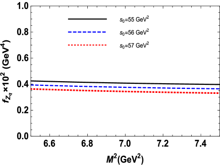
Figure 4: Left: The mass of the $Z_{q}$ state as a function of the Borel parameter $M^{2}$ at various values of $s_{0}$. Right: The meson-current coupling $f_{Z_{q}}$ as a function of the Borel parameter $M^{2}$ at different values of $s_{0}$.

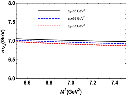
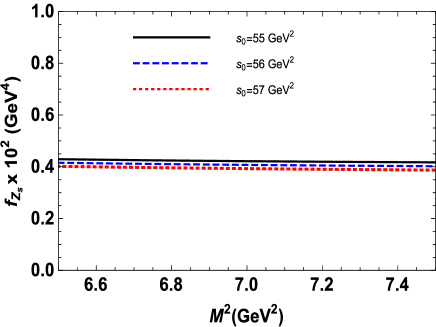
Figure 5: Left: The mass of the $Z_{s}$ state as a function of the Borel parameter $M^{2}$ at various values of $s_{0}$. Right: The meson-current coupling $f_{Z_{s}}$ as a function of the Borel parameter $M^{2}$ at different values of $s_{0}$.

From these figures we see that inside of the working windows for $M^{2}$ and $s_{0}$ , the mass sum rule demonstrates a good convergence and the perturbative part constitutes the main part of the total integral. We reach the PC contribution in the range $(16-31)\%$ for different values of $M^{2}$ and $s_{0}$ in their working regions. We shall also remark that the working regions for the Borel parameter and continuum threshold obtained for $Z_{q}$ state are roughly the same for $Z_{s}$ state and the $SU(3)$ flavor violation is negligible. Similar results for the convergence of OPE and pole contribution in $Z_{q}$ channel are obtained for $Z_{s}$ state as well and the presence of $s$ quark dose not change the situations in the figures 1- 3, considerably.

The results obtained for the mass and meson-current coupling of the $Z_{q}$ and $Z_{s}$ state are plotted in Figs. 4 and 5, and demonstrate mild dependence on $s_{0}$ and $M^{2}$. Our results for the masses and meson-current couplings of the $Z_{q}$ and $Z_{s}$ states are collected in Table 2. Here under $Z_{q}$ we imply both the $Z_{u}$ and $Z_{d}$ states, which in the exact isospin symmetry accepted in this work have identical physical parameters.

The masses of the scalar diquark-antidiquark states with the same contents were calculated in Ref. Chen:2013aba , as well. The authors used QCD two-point sum rule approach, and for the masses of the $Z_{s}$ and $Z_{q}$ states found:

$$m_{Z_{s}}=7.16\pm 0.08\pm 0.06\pm 0.04\,\,\mathrm{GeV},$$ (15)

and

$$m_{Z_{q}}=7.11\pm 0.08\pm 0.06\pm 0.01\,\,\mathrm{GeV}.$$ (16)

As is seen, obtained in this work predictions are consistent with our results within the errors: The slight discrepancies between the predictions of this study on the central values of masses of the states under consideration with our results can be attributed to the fact that in Ref. Chen:2013aba the authors do not take into account some terms in both the light and heavy quark propagators, which are taken into account in the present study. This leads to different working regions of the parameters $s_{0}$ and $M^{2}$ and different situation for the OPE convergence and pole/continuum contribution.

Mass, m.-c. coupling	Results
$m_{Z_{q}}$	$(6.97\pm 0.19)~{}\mathrm{GeV}$
$f_{Z_{q}}$	$(0.38\pm 0.03)\cdot 10^{-2}~{}\mathrm{GeV}^{4}$
$m_{Z_{s}}$	$(7.01\pm 0.21)~{}\mathrm{GeV}$
$f_{Z_{s}}$	$(0.41\pm 0.04)10^{-2}~{}\mathrm{GeV}^{4}$

Table 2: The two-point sum rule prediction for the masses and meson-current couplings of the $Z_{q}$ and $Z_{s}$ states.

III Widths of the $Z_{q}\to B_{c}\pi$, $Z_{q}\to B_{c}\eta$ and $Z_{s}\to B_{c}\eta$ decay channels

In this section we investigate the possible decay channels of the exotic $Z_{s(q)}$ states, and calculate the widths of the modes, which are, in accordance with our results obtained in Sec. II, kinematically allowed.

It is not dificult to see, that the quark content and mass of the $Z_{q}$ state permit its decay to $B_{c}$ and $\pi$ mesons: The producing of the $B_{c}$ and $\eta$ mesons in the decay process is also possible. The tetraquark $Z_{s}$ can decay to $B_{c}$ and $\eta$ mesons. At the same time, the modes $Z_{q}\to B_{c}\eta^{\prime}$ and $Z_{s}\to B_{c}\eta^{\prime}$ are among kinematically forbidden decay channels.

We concentrate here on the $Z_{s}\to B_{c}\eta$ decay channel. To find its width we explore the vertex $Z_{s}B_{c}\eta$ and calculate the strong coupling $g_{Z_{s}B_{c}\eta}$ using the light cone sum rule method and soft-meson approximation. To this end, we introduce the following correlation function

$$\Pi(p,q)=i\int d^{4}xe^{ipx}\langle\eta(q)|\mathcal{T}\{J^{B_{c}}(x)J^{{\dagger}}(0)\}|0\rangle,$$ (17)

where the interpolating current for the $B_{c}$ meson is given as

$$J^{B_{c}}(x)=i\overline{b}_{l}(x)\gamma_{5}c_{l}(x).$$ (18)

The correlation function $\Pi(p,q)$ is the basic component of the sum rule calculations. Expressed in terms of the physical quantities it takes a rather simple form

$$\Pi^{\mathrm{Phys}}(p,q) = \frac{\langle 0|J^{B_{c}}|B_{c}\left(p\right)\rangle}{p^{2}-m_{B_{c}}^{2}}\langle B_{c}\left(p\right)\eta(q)|Z_{s}(p^{\prime})\rangle$$ (19)

$$\times\frac{\langle Z_{s}(p^{\prime})|J^{\dagger}|0\rangle}{p^{\prime 2}-m_{Z}^{2}}+\ldots,$$

where $p$, $q$ and $p^{\prime}=p+q$ are the momenta of $B_{c}$, $\eta$, and the $Z_{s}$ states, respectively. The first term above is the ground state contribution, whereas effects of the higher resonances and continuum states are denoted by the dots.

We define the $B_{c}$ meson matrix element

$$\langle 0|J^{B_{c}}|B_{c}\left(p\right)\rangle=\frac{f_{B_{c}}m_{B_{c}}^{2}}{m_{b}+m_{c}},$$ (20)

with $m_{B_{c}}$ and $f_{B_{c}}$ being the mass and decay constant of the $B_{c}$ meson, and also the matrix element describing the vertex

$$\langle B_{c}\left(p\right)\eta(q)|Z_{s}(p^{\prime})\rangle=g_{Z_{s}B_{c}\eta}p\cdot p^{\prime}.$$ (21)

Then the ground state component of the correlation function can be recast into the form:

$$\Pi^{\mathrm{Phys}}(p,q)=\frac{f_{B_{c}}f_{Z}m_{Z}m_{B_{c}}^{2}g_{Z_{s}B_{c}\eta}}{\left(p^{\prime 2}-m_{Z}^{2}\right)\left(p^{2}-m_{B_{c}}^{2}\right)(m_{b}+m_{c})}p\cdot p^{\prime}.$$ (22)

In the soft-meson limit we apply the restriction $q=0$, which, naturally, leads to equality $p=p^{\prime}$ (for details, see Ref. Agaev:2016dev ). In this approximation the invariant function corresponding to $\Pi^{\mathrm{Phys}}(p,q)$ depends only on the variable $p^{2}$, and is given by the following expression

$$\Pi^{\mathrm{Phys}}(p^{2})=\frac{f_{B_{c}}f_{Z}m_{Z}m_{B_{c}}^{2}g_{Z_{s}B_{c}\eta}}{\left(p^{2}-m_{Z}^{2}\right)\left(p^{2}-m_{B_{c}}^{2}\right)(m_{b}+m_{c})}m^{2}$$

$$+\ldots,$$ (23)

where $m^{2}=\left(m_{Z}^{2}+m_{B_{c}}^{2}\right)/2.$

What is important, now we have to use the one-variable Borel transformation on $p^{2}$, and apply the operator

$$\left(1-M^{2}\frac{d}{dM^{2}}\right)M^{2}e^{m^{2}/M^{2}},$$ (24)

to both sides of the sum rule. The last operation is necessary to remove all unsuppressed contributions emerging in the physical side of the sum rule due to the soft-meson limit (see, Ref. Ioffe:1983ju ).

The second side of the sum rule, i.e. QCD expression for $\Pi^{\mathrm{QCD}}(p,q)$ is:

$$\Pi^{\mathrm{QCD}}(p,q)=i\int d^{4}xe^{ipx}\left\{\left[\gamma_{5}\widetilde{S}_{c}^{ib}(x){}\gamma_{5}\right.\right.$$

$$\left.\times\widetilde{S}_{b}^{bi}(-x){}\gamma_{5}\right]_{\alpha\beta}\langle\eta(q)|\overline{s}_{\alpha}^{a}s_{\beta}^{a}|0\rangle$$

$$\left.+\left[\gamma_{5}\widetilde{S}_{c}^{ib}(x)\gamma_{5}\widetilde{S}_{b}^{ai}(-x){}\gamma_{5}\right]_{\alpha\beta}\langle\eta(q)|\overline{s}_{\alpha}^{a}s_{\beta}^{b}|0\rangle\right\}.$$ (25)

Here by $\alpha$ and $\beta$ are the spinor indices.

We proceed by using the expansion

$$\overline{s}_{\alpha}^{a}s_{\beta}^{b}\rightarrow\frac{1}{4}\Gamma_{\beta\alpha}^{j}\left(\overline{s}^{a}\Gamma^{j}s^{b}\right),$$ (26)

where $\Gamma^{j}$ is the full set of Dirac matrixes, and performing the summation over color indices.

Calculation of the traces over spinor indices, and integration of the obtained integrals in accordance with procedures reported in Ref. Agaev:2016dev enable us to extract the imaginary part of the correlation function $\Pi^{\mathrm{QCD}}(p,q)$. As a result, we find not only the spectral density, but also determine local matrix elements of the $\eta$ meson that form it. Our analysis proves that in the soft-meson limit only the local twist-3 matrix element $\langle\eta(q)|\overline{s}i\gamma_{5}s|0\rangle$ survives and contributes to the spectral density $\rho_{\eta}^{s}(s)$ corresponding to the $Z_{s}B_{c}\eta$ vertex. Within the same approximation the strong couplings of the vertices $Z_{q}B_{c}\eta$ and $Z_{q}B_{c}\pi$ are determined by the matrix elements $\langle\eta(q)|\overline{q}i\gamma_{5}q|0\rangle$ and $\langle\pi(q)|\overline{q}i\gamma_{5}q|0\rangle$, respectively.

Situation with the pion is clear: its matrix element is known, and was used in our previous works to explore decays of other tetraquarks. But the matrix elements of the eta mesons deserve more detailed analysis, which is connected with mixing phenomena in the $\eta-\eta^{\prime}$ system.

The $\eta-\eta^{\prime}$ mixing and $U(1)$ axial anomaly are problems which decisively affect physics of the eta mesons. The $\eta-\eta^{\prime}$ mixing can be described using either the singlet-octet basis of the flavor group $SU_{f}(3)$, or the quark-flavor basis. The latter is founded on the $\bar{s}s$ and $(\bar{u}u+\bar{d}d)/\sqrt{2}$ as the basic states, and is convenient to describe the mixing phenomena of the $\eta-\eta^{\prime}$ system, including mixing of the physical states, decay constants and higher twist distribution amplitudes [Ref. Feldmann:1998vh ; Beneke:2002jn ; Agaev:2014wna ; Agaev:2015faa ].

In the present work we follow this approach and utilize the quark-flavor mixing scheme in our calculations. Then the twist-3 matrix elements of interest are given as

$$2m_{q}\langle\eta(q)|\overline{q}i\gamma_{5}q|0\rangle=\frac{h_{\eta}^{q}}{\sqrt{2}},$$ (27)

$$2m_{s}\langle\eta(q)|\overline{s}i\gamma_{5}s|0\rangle=h_{\eta}^{s},$$ (28)

where the parameters $h_{\eta}^{s(q)}$ are defined by the equalities

$$h_{\eta}^{s(q)} =m_{\eta}^{2}f_{\eta}^{s(q)}-A_{\eta}\,,$$

$$A_{\eta} =\langle 0|\frac{\alpha_{s}}{4\pi}G^{a}_{\mu\nu}\widetilde{G}^{a,\mu\nu}|\eta(p)\rangle,$$ (29)

and $A_{\eta}$ is the matrix element appeared due to the $U(1)$ anomaly .

In Refs. Beneke:2002jn ; Agaev:2014wna ; Agaev:2015faa it was assumed that the parameters $h_{\eta}^{s(q)}$ obey the same mixing scheme as the decay constants of the eta mesons, and hence the following equality holds:

$$\begin{pmatrix}h_{\eta}^{q}&h_{\eta}^{s}\\ h_{\eta^{\prime}}^{q}&h_{\eta^{\prime}}^{s}\end{pmatrix}=\begin{pmatrix}\cos\varphi&-\sin\varphi\\ \sin\varphi&\cos\varphi\end{pmatrix}\begin{pmatrix}h_{q}&0\\ 0&h_{s}\end{pmatrix}.$$ (30)

Here $\varphi$ is the mixing angle in the quark-flavor scheme, $h_{s}$ and $h_{q}$ are input parameters extracted from analysis of the experimental data:

$$h_{q}= (0.0016\pm 0.004)\,\,\mathrm{GeV}^{3},$$

$$h_{s}= (0.087\pm 0.006)\,\,\mathrm{GeV}^{3},$$

$$\varphi= 39.3^{\circ}\pm 1.0^{\circ}.$$ (31)

The details about the local matrix elements of the eta mesons presented above, is sufficient to calculate the spectral densities under investigation. We find:

$$\rho_{\eta}^{s}(s)=\frac{h_{\eta}^{s}}{48m_{s}}L(s),$$ (32)

for the $Z_{s}B_{c}\eta$ vertex,

$$\rho_{\eta}^{q}(s)=\frac{h_{\eta}^{q}}{48\sqrt{2}m_{q}}L(s),$$ (33)

for the $Z_{q}B_{c}\eta$ vertex, and

$$\rho_{\pi}(s)=\frac{f_{\pi}m_{\pi}^{2}}{24\sqrt{2}m_{q}}L(s)$$ (34)

for the $Z_{q}B_{c}\pi$ vertex, where the ”universal” function $L(s)$ has the form

$$L(s) = \frac{1}{\pi^{2}s^{2}}\left[s^{2}+s\left(m_{b}^{2}+6m_{b}m_{c}+m_{c}^{2}\right)-2(m_{b}^{2}-m_{c}^{2})^{2}\right]$$ (35)

$$\times \sqrt{\left(s+m_{b}^{2}-m_{c}^{2}\right)^{2}-4m_{b}^{2}s}+\frac{1}{3}\int\limits_{0}^{1}\frac{dz}{j^{2}z^{2}}$$

$$\times \left\{\langle\alpha_{s}\frac{G^{2}}{\pi}\rangle\left[s(m_{b}^{2}j^{3}+m_{b}m_{c}jz-m_{c}^{2}z^{3})\delta^{(2)}\left(s-\Phi\right)\right.\right.$$

$$+ \left.\left.2\left(m_{b}^{2}j^{3}-m_{c}^{2}z^{3}+m_{b}m_{c}(1+3jz)\right)\delta^{(1)}\left(s-\Phi\right)\right]\right.$$

$$+ \left.\langle g^{3}G^{3}\rangle\frac{1}{5\times 2^{6}\pi^{2}j^{3}z^{3}}\right.$$

$$\times \left.\left\{12j^{2}z^{2}\left[3m_{b}m_{c}(1+5jz(1+jz))\right.\right.\right.$$

$$+ \left.\left.\left.3m_{b}^{2}j^{5}-z\left(3m_{c}^{2}z^{4}+sj(1+jz(7+11jz))\right)\right]\right.\right.$$

$$\times \left.\left.\delta^{(2)}\left(s-\Phi\right)-2jz\left[m_{c}^{3}z^{5}(4m_{b}-7m_{c})\right.\right.\right.$$

$$+ \left.\left.\left.2s^{2}j^{3}z^{3}(2+7jz)+m_{b}^{2}j^{5}\left(7m_{b}^{2}-4m_{b}m_{c}\right.\right.\right.\right.$$

$$+ \left.\left.\left.\left.9s(1-2z)z\right)+9m_{c}sjz^{2}\left(m_{c}z^{3}(2z-1)\right.\right.\right.\right.$$

$$- \left.\left.\left.\left.2m_{b}j(1+3jz)\right)\right]\delta^{(3)}\left(s-\Phi\right)\right.\right.$$

$$+ \left.\left.\left[2m_{b}^{5}m_{c}j^{5}-2m_{c}^{5}m_{b}z^{5}-s^{3}j^{5}z^{5}+6s^{2}j^{3}z^{3}\right.\right.\right.$$

$$\times \left.\left.\left.\left(m_{b}^{2}j^{3}+m_{b}m_{c}jz-m_{c}^{2}z^{3}\right)+sjz\left(4m_{b}^{3}m_{c}j^{4}z\right.\right.\right.\right.$$

$$- \left.\left.\left.\left.7m_{b}^{4}j^{5}-4m_{c}^{3}m_{b}jz^{4}+7m_{c}^{4}z^{5}\right)\right]\delta^{(4)}\left(s-\Phi\right)\right\}\right.$$

$$+ \left.\langle\alpha_{s}\frac{G^{2}}{\pi}\rangle^{2}\frac{m_{b}m_{c}}{3^{3}\times 2}\left[-6jz\delta^{(3)}\left(s-\Phi\right)\right.\right.$$

$$+ \left.\left.2\left(m_{b}m_{c}-s(1+3jz)\right)\delta^{(4)}\left(s-\Phi\right)\right.\right.$$

$$+ \left.\left.s\left(m_{b}m_{c}-sjz\right)\delta^{(5)}\left(s-\Phi\right)\right]\right\},$$

where

$$\Phi = \frac{m_{b}^{2}j-m_{c}^{2}z}{jz},$$

$$j = z-1.$$ (36)

The final sum rule to evaluate the strong coupling reads

$$g_{Z_{s}B_{c}\eta}=\frac{(m_{b}+m_{c})}{f_{B_{c}}f_{Z}m_{Z}m_{B_{c}}^{2}m^{2}}\left(1-M^{2}\frac{d}{dM^{2}}\right)M^{2}$$

$$\times\int_{\mathcal{M}^{2}}^{s_{0}}dse^{(m^{2}-s)/M^{2}}\rho_{\eta}^{s}(s).$$ (37)

The similar expressions are valid for the remaining two couplings $g_{Z_{q}B_{c}\eta}$ and $g_{Z_{q}B_{c}\pi}$, as well.

In order to get the width of the decay $Z_{s}\to B_{c}\eta$ we adapt to this case the expression derived in Ref. Agaev:2016ijz , which takes the form

$$\Gamma\left(Z_{s}\to B_{c}\eta\right)=\frac{g_{Z_{s}B_{c}\eta}^{2}m_{B_{c}}^{2}}{24\pi}\lambda\left(m_{Z},\ m_{B_{c}},m_{\eta}\right)$$

$$\times\left[1+\frac{\lambda^{2}\left(m_{Z_{s}},\ m_{B_{c}},m_{\eta}\right)}{m_{B_{c}}^{2}}\right],$$ (38)

where

$$\lambda(a,\ b,\ c)=\frac{\sqrt{a^{4}+b^{4}+c^{4}-2\left(a^{2}b^{2}+a^{2}c^{2}+b^{2}c^{2}\right)}}{2a}.$$

Parameters required for numerical computations of the decay widths are listed in Table 1. Apart from the standard information it contains also the decay constant $f_{B_{c}}$ of the $B_{c}$ meson, for which we utilize its value derived in the context of the sum rule method in Ref. Baker:2013mwa .

The analysis carried out in accordance with traditional requirements of the sum rule calculations enable us to fix the working windows for the parameters $s_{0}$ and $M^{2}$ in this section. Our analyses show that the same regions for the $M^{2}$ and $s_{0}$ as the mass sum rules in the previous section lead to a better convergence of OPE and a nice pole contribution for the strong coupling constants under consideration. The perturbative-nonperturbative comparison, convergence of nonperturbative series and pole/total ratio as an example for $Z_{q}B_{c}\pi$ vertex are depicted in Figs. 6-8. From these figures we see that the perturbative contribution exceeds the nonperturbative one considerably and the OPE nicely converges. We also get a nice pole contribution of about $70\%$. Similar results are obtained for other vertices.

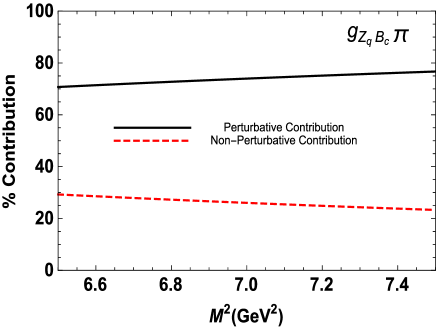
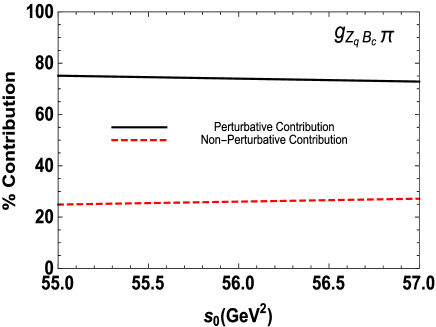
Figure 6: Left: Comparison of the perturbative and nonperturbative contributions to the $Z_{q}B_{c}\pi$ vertex with respect to $M^{2}$ at average value of $s_{0}$. Right: The same as left panel but in terms of $s_{0}$ at average value of the Borel parameter $M^{2}$.

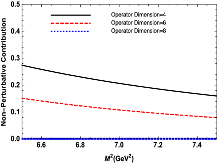
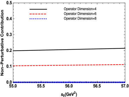
Figure 7: Left: Contribution of different nonperturbative operators to the $Z_{q}B_{c}\pi$ vertex with respect to $M^{2}$ at average value of $s_{0}$. Right: The same as left panel but in terms of $s_{0}$ at average value of the Borel parameter $M^{2}$.

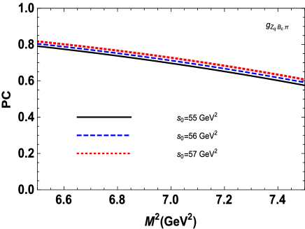
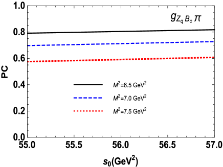
Figure 8: Left: Pole/total contribution of $Z_{q}B_{c}\pi$ vertex with respect to $M^{2}$ at different fixed values of $s_{0}$. Right: The same as left panel but in terms of $s_{0}$ at different fixed values of the Borel parameter $M^{2}$.

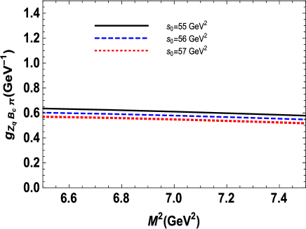
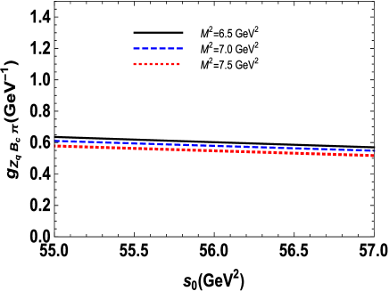
Figure 9: Left: The coupling constant $g_{Z_{q}B_{c}\pi}$ as a function of the Borel parameter $M^{2}$ at various values of $s_{0}$. Right: The coupling constant $g_{Z_{q}B_{c}\pi}$ as a function of threshold $s_{0}$ at various values of $M^{2}$.

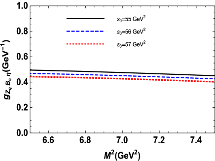
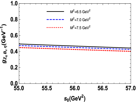
Figure 10: Left: The coupling constant $g_{Z_{q}B_{c}\eta}$ as a function of the Borel parameter $M^{2}$ at various values of $s_{0}$. Right: The coupling constant $g_{Z_{q}B_{c}\eta}$ as a function of threshold $s_{0}$ at various values of $M^{2}$.

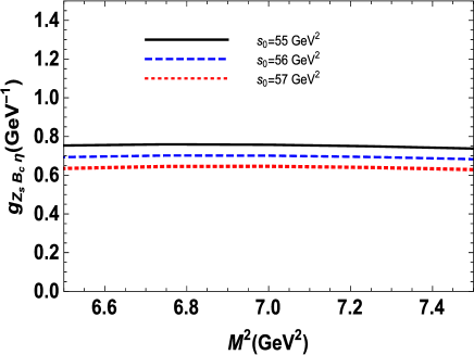
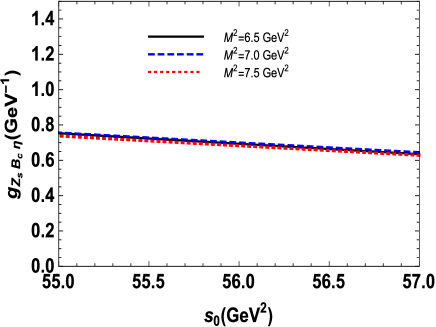
Figure 11: Left: The coupling constant $g_{Z_{s}B_{c}\eta}$ as a function of the Borel parameter $M^{2}$ at various values of $s_{0}$. Right: The coupling constant $g_{Z_{s}B_{c}\eta}$ as a function of threshold $s_{0}$ at various values of $M^{2}$.

Depicted in Figs. 9-11 output of numerical calculations demonstrates the dependence of the strong coupling constants, $g_{Z_{q}B_{c}\pi}$, $g_{Z_{q}B_{c}\eta}$ and $g_{Z_{s}B_{c}\eta}$ on $M^{2}$ and $s_{0}$, which demonstrate good instabilities of the couplings with respect to auxiliary parameters.

The strong couplings and decay widths of the exploring processes are collected in Table 3. The obtained results are typical for the decays of tetraquark states. One of their notable features is the difference between $\Gamma(Z_{q}\to B_{c}\pi)$ and $\Gamma(Z_{q}\to B_{c}\eta)$. In fact, the $Z_{q}$ state may interact with the pion and $\eta$ meson through its $\bar{q}q$ component. But the spectral density of the vertex $Z_{q}B_{c}\eta$ is proportional to $h_{\eta}^{q}$, which numerically is considerably smaller than $f_{\pi}m_{\pi}^{2}$ entering into $\rho_{\pi}(s)$. The reason is a reducing effect of the axial anomaly explicit from Eq. (29).

Strong couplings, Widths	Predictions
$g_{Z_{q}B_{c}\pi}$	$(0.57\pm 0.21)$ $\mathrm{GeV}^{-1}$
$g_{Z_{q}B_{c}\eta}$	$(0.45\pm 0.17)$ $\mathrm{GeV}^{-1}$
$g_{Z_{s}B_{c}\eta}$	$(0.69\pm 0.26)$ $\mathrm{GeV}^{-1}$
$\Gamma(Z_{q}\to B_{c}\pi)$	$(111\pm 49)$ $\mathrm{MeV}$
$\Gamma(Z_{q}\to B_{c}\eta)$	$(43\pm 19)$ $\mathrm{MeV}$
$\Gamma(Z_{s}\to B_{c}\eta)$	$(112\pm 51)$ $\mathrm{MeV}$

Table 3: The strong couplings and decay widths of the $Z_{q}$ and $Z_{s}$ exotic particles obtained within the soft-meson approximation.

Investigation of the open charm-bottom tetraquarks performed in the present work within the diquark-antidiquark picture led to quite interesting predictions. Theoretical exploration of these states using alternative pictures for their internal organization, as well as experimental studies may shed light not only on their parameters but also on properties of the conventional particles.

Appendix A The spectral densities for $Z_{q}$ state

Here we present the results obtained for the two-point spectral density corresponding to the $Z_{q}$ state. We get

$$\rho^{\mathrm{QCD}}(s)=\rho^{\mathrm{pert.}}(s)+\sum_{k=3}^{8}\rho_{k}(s),$$ (A.39)

where by $\rho_{k}(s)$ we denote the nonperturbative contributions to $\rho^{\mathrm{QCD}}(s)$. The explicit expressions for $\rho^{\mathrm{pert}}(s)$ and $\rho_{k}(s)$ are obtained in terms of the integrals of the Feynman parameters $z$ and $w$ as

$$\rho^{\mathrm{pert}}(s) = \frac{1}{2^{8}\pi^{6}}\int\limits_{0}^{1}dz\int\limits_{0}^{1-z}dw\frac{wz}{ht^{8}}\left(m_{b}^{2}tw+m_{c}^{2}tz-shwz\right)^{2}$$

$$\times \left[z^{2}\left(6m_{c}^{2}shtw-7s^{2}h^{2}w^{2}-m_{c}^{4}t^{2}\right)+2m_{b}^{2}twz\left(3shw-m_{c}^{2}t\right)-m_{b}^{4}t^{2}w^{2}\right]\Theta\left[L\left(s,z,w\right)\right],$$

$$\rho_{\mathrm{3}}(s) = \frac{\langle\overline{q}q\rangle}{2^{3}\pi^{4}}\int\limits_{0}^{1}dz\int\limits_{0}^{1-z}dw\frac{\left(m_{b}w+m_{c}z\right)}{t^{5}}\left(2shwz-m_{c}^{2}rz-m_{b}^{2}tw\right)\left(m_{b}^{2}tw+m_{c}^{2}rz-shwz\right)\Theta\left[L\left(s,z,w\right)\right],$$

$$\rho_{\mathrm{4}}(s) = -\frac{\langle\alpha_{s}\frac{G^{2}}{\pi}\rangle}{3\times 2^{9}\pi^{4}}\int\limits_{0}^{1}dz\int\limits_{0}^{1-z}dw\frac{wz}{ht^{6}}\left\{z^{2}\left[30h^{3}s^{2}w^{3}-4sm_{c}^{2}hrw\left(9pw+9wz+4z^{2}\right)\right.\right.$$

$$+ \left.\left.m_{c}^{4}r^{2}\left(9pw+9wz+8z^{2}\right)\right]+2m_{b}^{2}twz\left[m_{c}^{2}t\left(9wz+13w^{2}-9w+4z^{2}\right)-2shw^{2}\left(13w+9z-9\right)\right]\right.$$

$$+ \left.m_{b}^{4}t^{2}w^{3}\left(17w+9z-9\right)\right\}\Theta\left[L\left(s,z,w\right)\right],$$

$$\rho_{\mathrm{5}}(s) = \frac{m_{0}^{2}\langle\overline{q}q\rangle}{2^{5}\times\pi^{4}}\int\limits_{0}^{1}dz\int\limits_{0}^{1-z}dw\frac{h\left(m_{b}w+m_{c}z\right)}{t^{4}}\left(2m_{b}^{2}tw+2m_{c}^{2}rz-3shwz\right)\Theta\left[L\left(s,z,w\right)\right],$$

$$\rho_{\mathrm{6}}(s) = \frac{\langle g_{s}^{3}G^{3}\rangle}{5\times 3\times 2^{12}\pi^{6}}\int\limits_{0}^{1}dz\int\limits_{0}^{1-z}dw\frac{wz}{hf^{2}t^{7}}\left\{28m_{b}^{2}w^{7}f^{5}+zw^{6}f^{5}\left(32m_{b}^{2}+10m_{c}^{2}-21s\right)+w^{5}f^{4}z^{2}\right.$$

$$\times \left.\left[2m_{c}^{2}f+s\left(11w-32\right)+m_{b}^{2}\left(30w+2\right)\right]+2w^{4}z^{3}\left[3m_{b}^{2}j+2s-17m_{b}^{2}w-m_{c}^{2}f^{4}(3w-4)\right.\right.$$

$$+ \left.\left.m_{b}^{2}w^{2}(38-42w+23w^{2}-5w^{3})+2s(11-54w+86w^{2}-59w^{3}+15w^{4})\right]-2w^{3}z^{4}\right.$$

$$\times \left.\left[j^{2}(m_{b}^{2}(19w-4)-3m_{c}^{2}-2s)-2sw(w^{2}-2)(4-7w+4w^{2})+m_{b}^{2}w^{2}(10w^{3}-43w^{2}+73w-61)\right.\right.$$

$$+ \left.\left.m_{c}^{2}w(23-62w+78w^{2}-47w^{3}+11w^{4})\right]+2w^{2}z^{5}\left[m_{b}^{2}j+m_{c}^{2}j^{2}(1-7w)+3m_{b}^{2}j^{2}w(4w-1)\right.\right.$$

$$+ \left.\left.2sj^{2}(31w-8)+m_{b}^{2}w^{3}(56w-14w^{2}-83)+m_{c}^{2}w^{2}(46-70w+49w^{2}-13w^{3})+2sw^{2}(5w+13w^{2}\right.\right.$$

$$- \left.\left.6w^{3}-33)\right]+z^{6}w\left[j^{3}(21s-32m_{c}^{2}+2m_{b}^{2}(6w-5))+j^{2}w(12m_{b}^{2}w(f+w)+s(25+22w)\right.\right.$$

$$+ \left.\left.m_{c}^{2}(78w-90))+w^{3}(2m_{c}^{2}(f-1)(11f-5)+2m_{b}^{2}w(16w-51)+s(163w-19w^{2}-350))\right]\right.$$

$$- \left.z^{7}\left[s(228w^{4}-75w^{5})+26m_{b}^{2}w^{5}+20m_{c}^{2}w^{5}-2j^{2}w^{2}\left(3m_{c}^{2}(f-10)-5m_{b}^{2}w+3s(3+w)\right)\right.\right.$$

$$+ \left.\left.2j^{3}\left(2m_{c}^{2}(12w-7)+3sw+m_{b}^{2}w(5w-2)\right)\right]+z^{8}\left[j^{2}w^{2}(8m_{c}^{2}+15s)+2w^{4}(19s+5m_{c}^{2})\right.\right.$$

$$+ \left.\left.j^{3}\left(m_{c}^{2}(4-10w)-2m_{b}^{2}w+3sw\right)\right]-2j^{3}z^{9}m_{c}^{2}\right\}\Theta\left[L\left(s,z,w\right)\right]$$

$$+ \frac{g_{s}^{2}\langle\overline{q}q\rangle^{2}}{3^{2}\times 2\pi^{4}}\int\limits_{0}^{1}dz\int\limits_{0}^{1-z}dw\frac{h^{2}wz}{t^{5}}\left(2shwz-m_{b}^{2}tw-m_{c}^{2}tz\right)\Theta\left[L\left(s,z,w\right)\right]$$

$$+ \frac{\langle\overline{q}q\rangle^{2}}{6\pi^{2}}\frac{m_{b}m_{c}}{s}\sqrt{(s+m_{b}^{2}-m_{c}^{2})^{2}-4sm_{b}^{2}},$$

$$\rho_{\mathrm{7}}(s) = \frac{\langle\alpha_{s}\frac{G^{2}}{\pi}\rangle\langle\overline{q}q\rangle}{3^{2}\times 2^{5}\pi^{2}}\left\{\int\limits_{0}^{1}dz\int\limits_{0}^{1-z}dw\frac{1}{\left[w^{2}+j(w+z)\right]^{4}}\left\{4m_{b}w^{3}(z^{2}+zf-2wf)+m_{c}z\left[fwz(3-2z-6w)\right.\right.\right.$$

$$+ \left.\left.\left.z^{3}(w-8z+8)-3f^{2}w^{2}\right]\right\}\Theta\left[L\left(s,z,w\right)\right]+\frac{m_{b}+m_{c}}{s^{2}}\left[(m_{b}-m_{c})^{2}-s\right]\sqrt{(m_{b}^{2}-m_{c}^{2}+s)^{2}-4sm_{b}^{2}}\right\},$$

$$\rho_{\mathrm{8}}(s) = -\frac{\langle\alpha_{s}\frac{G^{2}}{\pi}\rangle^{2}}{3^{4}\times 2^{9}\pi^{2}}\int\limits_{0}^{1}dz\int\limits_{0}^{1-z}dw\frac{m_{b}^{2}m_{c}^{2}wz}{h^{4}t^{2}f}\left\{hfwz\left[10\delta^{(1)}\left(s-\Delta\right)+11\delta^{(2)}\left(s-\Delta\right)\right]+2s^{2}t^{2}\delta^{(3)}\left(s-\Delta\right)\right\},$$ (A.40)

where we omitted to show the terms proportional to the $m_{q}$ in order to avoid from very lengthy expressions. Here,

$$L\left(s,z,w\right) = -\frac{f\left[j(w+z)(m_{b}^{2}w+m_{c}^{2}z)+w(m_{b}^{2}w^{2}-shz+m_{c}^{2}wz)\right]}{\left(w^{2}+j(w+z)\right)^{2}},$$

$$\delta^{(n)}\left(s-\Delta\right) = \left(\frac{d}{ds}\right)^{n}\left(s-\Delta\right),$$

$$\Delta = \frac{t(m_{b}^{2}w+m_{c}^{2}z)}{hwz},$$

$$t = w^{2}+(w+z)(z-1),$$

$$r = z^{2}+(w+z)(w-1),$$

$$h = w+z-1,$$

$$f = w-1,$$

$$j = z-1,$$ (A.41)

and $\Theta\left[...\right]$ is the usual unit-step function.

References

- (1) S.-K. Choi et al. [Belle Collaboration], Phys. Rev. Lett. 91, 262001 (2003).
- (2) V. M. Abazov et al. [D0 Collaboration], Phys. Rev. Lett. 93, 162002 (2004); D. Acosta et al. [CDF II Collaboration] Phys. Rev. Lett. 93, 072001 (2004); B. Aubert et al. [BaBar Collaboration], Phys. Rev. D 71, 071103 (2005).
- (3) E. S. Swanson, Phys. Rept. 429, 243 (2006).
- (4) E. Klempt and A. Zaitsev, Phys. Rept. 454, 1 (2007).
- (5) S. Godfrey and S. L. Olsen, Ann. Rev. Nucl. Part. Sci. 58, 51 (2008).
- (6) M. B. Voloshin, Prog. Part. Nucl. Phys. 61, 455 (2008).
- (7) M. Nielsen, F. S. Navarra, and S. H. Lee, Phys. Rep. 497, 41 (2010).
- (8) R. Faccini, A. Pilloni and A. D. Polosa, Mod. Phys. Lett. A 27, 1230025 (2012).
- (9) A. Esposito, A. L. Guerrieri, F. Piccinini, A. Pilloni and A. D. Polosa, Int. J. Mod. Phys. A 30, 1530002 (2015).
- (10) C. A. Meyer and E. S. Swanson, Prog. Part. Nucl. Phys. 82, 21 (2015)
- (11) H. X. Chen, W. Chen, X. Liu and S. L. Zhu, Phys. Rept. 639, 1 (2016).
- (12) R. F. Lebed, R. E. Mitchell and E. S. Swanson, arXiv:1610.04528 [hep-ph].
- (13) V. M. Abazov et al. [D0 Collaboration], Phys. Rev. Lett. 117, 022003 (2016).
- (14) The D0 Collaboration, D0 Note 6488-CONF, (2016).
- (15) R. Aaij et al. [LHCb Collaboration], Phys. Rev. Lett. 117, 152003 (2016).
- (16) The CMS Collaboration, CMS PAS BPH-16-002, (2016).
- (17) H. X. Chen, W. Chen, X. Liu, Y. R. Liu and S. L. Zhu, arXiv:1609.08928 [hep-ph].
- (18) J. R. Zhang and M. Q. Huang, Phys. Rev. D 80, 056004 (2009).
- (19) J. R. Zhang and M. Q. Huang, Commun. Theor. Phys. 54, 1075 (2010)
- (20) Z. F. Sun, X. Liu, M. Nielsen and S. L. Zhu, Phys. Rev. D 85, 094008 (2012)
- (21) R. M. Albuquerque, X. Liu and M. Nielsen, Phys. Lett. B 718, 492 (2012)
- (22) S. Zouzou, B. Silvestre-Brac, C. Gignoux and J. M. Richard, Z. Phys. C 30, 457 (1986).
- (23) B. Silvestre-Brac and C. Semay, Z. Phys. C 59, 457 (1993).
- (24) W. Chen, T. G. Steele and S. L. Zhu, Phys. Rev. D 89, 054037 (2014).
- (25) M. A. Shifman, A. I. Vainshtein and V. I. Zhakharov, Nucl. Phys. B 147, 385 (1979).
- (26) V. M. Braun and A. V. Kolesnichenko, Phys. Lett. B 175, 485 (1986) [Sov. J. Nucl. Phys. 44, 489 (1986)] [Yad. Fiz. 44, 756 (1986)].
- (27) V. M. Braun and Y. M. Shabelski, Sov. J. Nucl. Phys. 50, 306 (1989) [Yad. Fiz. 50, 493 (1989)].
- (28) I. I. Balitsky, D. Diakonov and A. V. Yung, Phys. Lett. B 112, 71 (1982); Z. Phys. C 33, 265 (1986).
- (29) J. Govaerts, L. J. Reinders, H. R. Rubinstein and J. Weyers, Nucl. Phys. B 258, 215 (1985);J. Govaerts, L. J. Reinders and J. Weyers, Nucl. Phys. B 262, 575 (1985).
- (30) I. I. Balitsky, V. M. Braun, A. V. Kolesnichenko, Nucl. Phys. B 312, 509 (1989).
- (31) B. L. Ioffe and A. V. Smilga, Nucl. Phys. B 232, 109 (1984).
- (32) V. M. Belyaev, V. M. Braun, A. Khodjamirian and R. Rückl, Phys. Rev. D 51, 6177 (1995).
- (33) S. S. Agaev, K. Azizi and H. Sundu, Phys. Rev. D 93, 074002 (2016).
- (34) S. S. Agaev, K. Azizi and H. Sundu, Phys. Rev. D 93, 114007 (2016).
- (35) S. S. Agaev, K. Azizi and H. Sundu, Phys. Rev. D 93, 094006 (2016).
- (36) S. S. Agaev, K. Azizi and H. Sundu, Eur. Phys. J. Plus 131, 351 (2016).
- (37) S. S. Agaev, K. Azizi and H. Sundu, Phys. Rev. D 93, 114036 (2016).
- (38) A. K. Agamaliev, T. M. Aliev and M. Savcı, arXiv:1610.03980 [hep-ph].
- (39) L. J. Reinders, H. Rubinstein and S. Yazaki, Phys. Rept. 127, 1 (1985).
- (40) S. S. Agaev, K. Azizi and H. Sundu, Phys. Rev. D 93, 074024 (2016).
- (41) S. Narison, Nucl. Part. Phys. Proc. 270-272, 143 (2016).
- (42) C. Patrignani, Chin. Phys. C 40, 100001 (2016).
- (43) T. Feldmann, P. Kroll and B. Stech, Phys. Rev. D 58, 114006 (1998); Phys. Lett. B 449, 339 (1999).
- (44) M. Beneke and M. Neubert, Nucl. Phys. B 651, 225 (2003).
- (45) S. S. Agaev, V. M. Braun, N. Offen, F. A. Porkert and A. Schafer, Phys. Rev. D 90, 074019 (2014).
- (46) S. S. Agaev, K. Azizi and H. Sundu, Phys. Rev. D 92, 116010 (2015)
- (47) M. J. Baker, J. Bordes, C. A. Dominguez, J. Penarrocha and K. Schilcher, JHEP 1407, 032 (2014).