Weak Measurement and Two-State-Vector Formalism: Deficit of Momentum Transfer in Scattering Processes

The notions of weak measurement, weak value, and two-state-vector formalism provide a new quantum-theoretical frame for extracting additional information from a system in the limit of small disturbances to its state. Here, we provide an application to the case of two-body scattering with one body weakly interacting with an environment. The direct connection to real scattering experiments is pointed out by making contact with the field of impulsive incoherent neutron scattering from molecules and condensed systems. In particular, we predict a new quantum effect in neutron-atom collisions, namely an observable momentum transfer deficit; or equivalently, a reduction of effective mass below that of the free scattering atom. Two corroborative experimental findings are shortly presented. Implications for current and further experiments are mentioned. An interpretation of this effect and the associated experimental results within conventional theory is currently unavailable.
Quanta 2016; 5: 61–84.

 
This is an open access article distributed under the terms of the Creative Commons Attribution License CC-BY-3.0, which permits unrestricted use, distribution, and reproduction in any medium, provided the original author and source are credited.

1 Introduction

Time symmetry, and the associated microscopic reversibility, is widely acknowledged to be a fundamental property of the basic physical laws of classical and quantum mechanics [1]. In contrast, the Second Law of thermodynamics, although also being considered fundamental, is inconsistent with this symmetry and provides an arrow of time associated with entropy production appearing in isolated many-body systems. However, thermodynamics and statistical mechanics (classical or quantum), and the associated thermodynamic limit (when the particle number $N\rightarrow\infty$) are not under consideration in this paper. Instead, here we are particularly interested in (few-body) quantum dynamics in connection with quantum measurements [2, 3, 4], in the realm of non-relativistic quantum mechanics. In particular, the emphasis will be on an experimental application in the frame of incoherent scattering experiments. (An explanation from first principles of coherent versus incoherent, being also helpful for the neutron-proton scattering experiments considered below, was presented by Feynman in [1, Section 3-3].)

In this context, the irreversible character of the standard (i.e. projective, strong) measurements should be mentioned. In contrast with the unitary (and thus time-symmetric) time evolution generated by the Schrödinger equation, a strong (projective) measurement [2, 3, 4] causes a reduction of the state of the measured system, constituting an irreversible (i.e. time-oriented) process.

Environmentally induced decoherence (see e.g. the textbooks [4, 5]) breaks time symmetry of the equations of motion and thus provides an explanation for the appearance of time-oriented quantum processes in open quantum systems. Nowadays decoherence plays a crucial role in many fields of physics, chemistry and molecular biology, in quantum information theory and also in the currently emerging quantum information technologies, e.g. quantum computing, communication and coding [4].

Novel insights into the measurement problem of quantum mechanics, and hence also into the foundations of quantum theory, are provided by the seminal work by Aharonov and collaborators, commonly known as theory of weak measurements and/or weak values; see e.g. the textbook [6] and the review article [7]. Elegant introductory presentations are given in [8, 9, 10]. For a very recent discussion of the basic physical aspects, see [11].

The outline of this article is as follows: In Section 2, we begin by briefly reviewing some basic elements of the aforementioned theoretical frame, since it plays a central role in the physical context of the present paper. Section 3 presents a few theoretical papers that motivated the application of the weak measurement theory to the scattering topic being under consideration in this paper. In Section 4 are presented basic elements of the theory of impulsive scattering and the specific experimental method employed to a class of neutron scattering experiments (as those presented in Section 6). Section 5, which is the main theoretical part of the paper, investigates elementary scattering in the light of weak measurement and two-state-vector formalism [6, 8, 9, 11]. The main theoretical result is the effect of momentum transfer deficit in impulsive collisions, and associated aspects of it (e.g. the anomalous reduction of effective mass of the scattering particle, or an increased energy transfer). Two concrete neutron scattering experiments demonstrating the experimental applicability of the weak measurement theory, as well as its novelty, are presented in Section 6. Finally, Section 7 provides additional remarks to the main results and a discussion.

Here, it may be helpful to emphasize two particularly relevant points. First, what we directly read out in a measurement of an experiment are not (values of) the dynamical variables of the observed system, but the outcomes of the measuring devices of the employed instrument (see subsection 7.1). To these outcomes belongs the measured data (in Section 6) that exhibits the peculiar phenomenon of momentum transfer deficit. It will be demonstrated that the latter contradicts every prediction of conventional theory even qualitatively, but it can be interpreted straightforwardly within the theory of weak values and two-state-vector formalism.

Second, with respect to an important point raised by Vaidman [12], we would like to stress the following special feature of our investigation. Until now, weak values are measured with a different degree of freedom of the same quantum system. Here, however, a weak value is observed with an external quantum system. Hence, in the present investigation, the weak value appears due to interference of a quantum entangled wave, thus having no analog in classical wave interference [12].

2 On weak measurement, post-selection and two-state-vector formalism

Weak measurement is unique in measuring non-commuting operators and revealing new counter-intuitive effects predicted by the new theory of weak values and two-state-vector formalism [11, 13, 14]. The main aim of this article is not to further develop and/or extend this theory, but to point out certain new (and experimentally observable) features of elementary scattering processes predicted within the theoretical frame of weak values and two-state-vector formalism. Especially, incoherent scattering of single (massive) particles, like neutrons or electrons, from nuclei and/or atoms is investigated.

As the starting point of the aforementioned theory one usually considers the paper [15] by Aharonov, Albert and Vaidman, and the earlier paper [16] by Aharonov, Bergmann and Lebowitz; see also [17] for a clarifying discussion. Here let us shortly mention a few results needed in the following.

According to the standard theory (of ideal, projective von Neumann measurements [18]), the final state of the system after a measurement becomes an eigenstate of the measured observable. This usually disturbs the state of the system. On the other hand, by coupling a measuring device to a system sufficiently weakly, it may be possible to read out certain information while limiting the disturbance induced by the measurement to the system. As Aharonov and collaborators originally proposed [15, 16], one may achieve new physical insights when one furthermore post-selects on a particular outcome of the experiment. In this case the eigenvalues of the measured observable are no longer the relevant quantities; rather the measuring device consistently indicates the weak value given by [15, 16]

$$A_{w}\equiv(\hat{A})_{w}=\frac{\langle\psi_{f}|\hat{A}|\psi_{i}\rangle}{\langle\psi_{f}|\psi_{i}\rangle},$$ (1)

where $\hat{A}$ is the operator of the quantity being measured, $|\psi_{i}\rangle$ is the initial (pre-selected) state of the system, and $|\psi_{f}\rangle$ is the post-selected state after the weak measurement. Note that the number $A_{w}$ may be complex.

The significance of this formula is as follows. Let us couple a measuring device whose pointer has position coordinate $\hat{q}$ to the system’s dynamical variable $\hat{A}$, and subsequently measure its conjugated momentum $\hat{p}$. The coupling interaction is taken to be the standard von Neumann measurement interaction [18]

$$\hat{H}_{\textrm{vN}}=-g(t)\,\hat{q}\otimes\hat{A}.$$ (2)

The coupling factor $g(t)$ is assumed to be appropriately small and to have a compact support at the time of the (impulsive) measurement; e.g. it may be proportional to a delta function. Since it is time-dependent, the complete Hamiltonian of the system and the measuring device represents an open quantum system. Consequently, in the situations contemplated here the time dependence of the coupling constant implies that energy conservation need not apply.

The mean value $\langle\hat{p}\rangle_{f}$ of the pointer momentum after the measurement is given by [15]

$$\langle\hat{p}\rangle_{f}-\langle\hat{p}\rangle_{i}=+g\,\textrm{Re}[A_{w}],$$ (3)

where $\langle\hat{p}\rangle_{i}$ is the corresponding value before measurement, Re denotes the real part and $g=\int g(t)dt$.

Formula (1) implies that, if the initial state $|\psi_{i}\rangle$ is an eigenstate of a measurement operator $\hat{A}$, then the weak value post-conditioned on that eigenstate is the same as the classical (strong) measurement result. When there is a definite outcome, therefore, strong and weak measurements agree. However, a weak measurement can yield values outside the range of measurement results predicted by conventional theory [15].

A weak value can also be complex, with an imaginary part corresponding to the pointer position. In fact, the mean of the pointer position after measurement is given by

$$\langle\hat{q}\rangle_{f}=-2gv_{q}\ \textrm{Im}[A_{w}],$$ (4)

where Im denotes the imaginary part and $v_{q}$ is the variance in the initial pointer spatial position [15], assuming that $\langle\hat{q}\rangle_{i}=0$ before measurement.

In the simplest case where there is just one observable $\hat{A}$, we assume the evolution from $|\psi_{i}\rangle$ to the point where $\hat{A}$ is measured is given by $\hat{U}$, and from this point to the post-selection the evolution is given by $\hat{V}$. Then we can rewrite formula (1) as:

$$A_{w}\equiv(\hat{A})_{w}=\frac{\langle\psi_{f}|\hat{V}\hat{A}\hat{U}|\psi_{i}\rangle}{\langle\psi_{f}|\hat{V}\hat{U}|\psi_{i}\rangle}$$ (5)

and the expressions (3) and (4) characterizing the pointer shift remain valid.

The fact that one only sufficiently weakly disturbs the system in making weak measurements implies that one can in principle measure different (also non-commuting) dynamical variables in succession. This theoretical observation has led to a great number of experimental applications and discovery of several new effects; see e.g. [19, 20, 21, 22, 36].

The generalization of the concept of weak value to a system described by a density operator $\hat{\rho}_{i}$ (for its initial state) was first considered by Wiseman [23]:

$$(\hat{A})_{w}=\frac{\langle\psi_{f}|\hat{A}\hat{\rho}_{i}|\psi_{f}\rangle}{\langle\psi_{f}|\hat{\rho}_{i}|\psi_{f}\rangle};$$ (6)

cf. also [24].

Furthermore, it may be noted that there is (steadily growing) evidence that the weak value formalism can be extended beyond the weak coupling regime of the original framework [15]; see e.g. [7, 25, 26]. Moreover, recently it has been shown that measurements on macroscopic systems are weak measurements [27], which also provided new physical inside to quantum non-locality [27, 28].

Technical and experimental merits, and associated advantages (or disadvantages) to precision metrology, of weak values-based techniques have been discussed in various works, e.g. in [29, 30].

Although a discussion and/or analysis of the physical interpretation and/or meaning of the concepts of weak values and two-state-vector formalism are beyond the scope of this paper, a few related short remarks may be in order.

Nowadays, the importance of weak values and associated weak measurement as a practical tool for describing new experiments and extract new information from experiments seems to be broadly acknowledged; cf. the discussions in [10]. However, various criticisms have been provided which deny or question the novelty of these quantum mechanical concepts. For example, in [31] it is claimed that weak value is not an inherently quantum concept but rather a purely statistical feature of pre- and post-selection with disturbance; and furthermore, that classical correlation alone supplies the surprising anomalies revealed with weak values. For some concise comments stressing quite the opposite, see [12, 32].

For the interpretation of the experimental findings presented below, it is relevant that weak values are novel quantum interference phenomena, having no classical analogue, in which post-selection plays a crucial role; cf. [12, 32, 33, 34, 35, 37].

3 Some previous results and motivation

This paper concerns the measurement of momentum and energy transfers in real scattering experiments, the corresponding predictions of conventional theory, and a new prediction based on the formalism of weak measurement and two-state-vector formalism. The latter point may be best illustrated and motivated by referring directly to some of the intriguing results presented in two recent papers [36, 38]. Additionally, we mention here certain interpretational issues concerning the theoretical status of weak values [12], because they contributed to the motivation of the present investigation and facilitate the interpretation of the obtained results.

First, let us refer to a surprising theoretical prediction derived by Aharonov et al. in [38], which may be shortly described (with some simplifications) as follows.

A photon beam enters a device similar to a usual Mach–Zehnder interferometer, with the exception that one reflecting mirror is sufficiently small (say, a nanoscopic object $M$) for its momentum distribution to be detectable by a suitable non-demolition measurement [39]. The two identical beam splitters of the Mach–Zehnder interferometer have nonequal reflectivity $r$ and transmissivity $t$ (both real, with $r^{2}+t^{2}=1$), say $r>t$. Now one is interested in the momentum kicks given to the mirror $M$ caused by the photon reflection on $M$ inside the interferometer, but only for photons emerging toward one of the two detectors (D₂ in Fig. 2 of [38]). The latter condition is a specific post-selection. The effect of the photons emerging toward the second detector is discarded.

A straightforward calculation [38] shows the following astonishing feature. Although the post-selected photons collide (as all photons do, of course) with the mirror $M$ only from the inside of the Mach–Zehnder interferometer, they do not push $M$ outwards, but rather they somehow succeed to pull it in. It is obvious that this result cannot have any conventional theoretical interpretation. As Aharonov et al. put it:

This is realized by a superposition of giving the mirror zero momentum and positive momentum—the superposition results in the mirror gaining negative momentum. [38]

Another paper by Vaidman and collaborators [36] presents experimental and theoretical results of optical measurements with a special interferometer being a combination of two Mach–Zehnder interferometers; essentially, a second Mach–Zehnder interferometer is put on the place of one of the two reflecting mirrors of the first Mach–Zehnder interferometer. The whole construction consists of 5 mirrors and 4 beam splitters (see [36, Figs. 2(b) and 3]). A continuous laser beam enters the interferometer.

Furthermore, all 5 mirrors are placed on piezoelectrically driven mirror mounts and are weakly vibrating at different frequencies (say $f_{i}$) and produce very slight rotational motions, which correspondingly produce slight deflections of the photon beam. The vertical displacements of the beam due to the vibrations of the mirrors are significantly smaller than the width of the beam, and the change in the optical path length is much smaller than the wavelength. The photon beam coming out of the interferometer (toward a specific detector) is measured and Fourier analyzed. It is natural to expect that the specific frequencies appearing in the Fourier power spectrum should be those of the mirrors the photons bounce off.

The reported experimental results are quite unexpected. For example, in one specific setup (see [36, Fig. 3]), three frequencies (i.e. those of mirrors A, B and C) appear in the measured power spectrum instead of the naturally expected one frequency (i.e. that of mirror C). Moreover, it appears that the past of the photons is not represented by continuous trajectories.

However, these striking results have a simple explanation in the framework of two-state-vector formalism. As Vaidman et al. propose, the intuitive picture which allows us to understand the experimental findings is provided by the time-symmetric two-state-vector formalism. Here each photon observed by detector ($D$ in [36, Fig. 3]) is described by the backward-evolving quantum state $\langle\psi_{f}|$ post-selected at $D$, in addition to the standard, forward-evolving wave function $|\psi_{i}\rangle$ pre-selected at the photon source. The formulas of two-state-vector formalism imply that a photon can have a local observable effect only if both the forward- and backward-evolving quantum waves are non-vanishing at the considered location; see [36, Fig. 3], in which both forward-in-time and backward-in-time paths of traveling photons are shown.

In other terms, one may say that each photon was present in a specific position (i.e. at a specific mirror) only when both forward- and backward-evolving quantum wave functions do not vanish at that position—this happens only at three of the five mirrors. This provides an explanation from first principles of the observed power spectrum in the frame of two-state-vector formalism, thus also illustrating the predictive power of the theory.

Responding to certain claims that question the novelty of weak values, Vaidman states the following:

The weak value shifts exist if measured or not, so the weak value is not defined by the statistics of measurement outcomes. The statistical analysis (performed after the post-selection) can just reveal the pre-existing weak values. $\left[\ldots\right]$
The concept of weak value arises due to wave interference and has no analog in classical statistics. Moreover, if weak values are observed with external systems (and not with a different degree of freedom of the observed system as it has been done until now) then the weak value appears due to interference of a quantum entangled wave and it has no analog in classical wave interference too. Therefore, weak value is a genuinely quantum concept [12].

Concluding the above short remarks, one may say that the new insights and predictions made possible within the theoretical frame of weak measurement, weak values and two-state-vector formalism are not limited to interpretational issues only. The revised intuitions can then lead one to find novel quantum effects that can be measured in real experiments.

4 Elementary remarks on impulsive scattering

Throughout this paper non-relativistic quantum mechanics is considered. In this section, we give an outline of basic elements of impulsive scattering experiments. In particular, we consider incoherent inelastic neutron scattering from condensed matter (see the textbooks [40, 41]) and its specification to high momentum transfers, known as neutron Compton scattering or deep-inelastic neutron scattering; cf. [42, 43, 44]. (The neutron-nucleus collision is elastic; “inelastic” simply refers to the decreased kinetic energy of the neutron’s final state; see Eq. (8).) The initial energy of the neutrons under consideration is roughly in the range of meV (for cold neutrons) until about 100 eV (for epithermal neutrons). The de Broglie wavelength of the neutrons is roughly in the range 0.1–10 Å. In two-body (i.e. neutron-nucleus) collisions, the scattering is isotropic in the center-of-mass system, which is called $s$-wave scattering. This is because the range of the nuclear strong force, and also the dimension of nuclei, are some orders of magnitude smaller than neutron’s de Broglie wavelength.

The usual experimental method employed at pulsed neutron sources is time-of-flight; see below.

A similar outline applies also to electron Compton-like quasielastic scattering from atoms (or molecules) in the gas phase; see e.g. [45]. In a conventional electron scattering spectrometer, instead of time-of-flight, the experimental method uses the deflection of the scattered electron in an electric field, in order to determine the electron’s final energy. However, a new generation of instruments provides pulsed electron beams and applies the time-of-flight analysis; cf. [46].

4.1 Scattering experimental setup – What is measured

First, let us give an outline of a standard time-of-flight scattering experiment; see Fig. 1. A pulsed source of particles, say neutrons, is used. A short pulse reaches the monitor which triggers the measurement of time-of-flight. A neutron scatters from the sample and reaches the detector, which stops the time-of-flight measurement. For a measured time-of-flight value $t_{\textrm{TOF}}$ holds

$$t_{\textrm{TOF}}=\frac{L_{0}}{v_{0}}+\frac{L_{1}^{\theta}}{v_{1}}+t_{0}.$$ (7)

Here, $L_{0}$ is the distance between source and sample, $L_{1}^{\theta}$ is the sample–detector distance; the detector is positioned at the scattering angle $\theta$; $v_{0}$ and $v_{1}$ describe the neutron’s velocities before and after scattering, respectively; $t_{0}$ is a (usually small) time offset arising due to electronic delays. In a so-called direct geometry spectrometer, the energy of the incident neutrons is chosen as constant, $E_{0}=$constant.

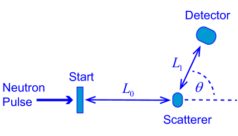
Figure 1: Schematic of a time-of-flight scattering experiment.

In a general scattering experiment the scattering intensity is measured as a function of the neutron energy transfer (or: energy loss)

$$E = E_{0}-E_{1}=\frac{1}{2}mv_{0}^{2}-\frac{1}{2}mv_{1}^{2}$$ (8)

$$= \hbar\omega=\frac{(\hbar k_{0})^{2}}{2m}-\frac{(\hbar k_{1})^{2}}{2m}$$

($m$: neutron mass) due to the neutron-atom collision, and the corresponding neutron momentum transfer on the struck atom

$$\hbar{\mathbf{K}}=\hbar{\mathbf{k}}_{0}-\hbar{\mathbf{k}}_{1},$$ (9)

where

$$|{\mathbf{K}}|=K=\sqrt{k_{0}^{2}+k_{1}^{2}-2k_{0}k_{1}\cos\theta}.$$ (10)

The subscripts 0 and 1 refer to quantities before and after the neutron-atom collision, respectively. Since the scattering under consideration is incoherent [1], it causes exchange of momentum between a neutron and (the nucleus of) a single atom.

In the standard theory of elastic scattering from a free atom with mass $M$ and zero initial momentum, $\langle P\rangle=0$, conservation of kinetic energy and momentum in an elastic neutron-atom collision yield the simple kinematic relation [43]

$$\frac{k_{1}}{k_{0}}=\frac{\cos\theta+\sqrt{(M/m)^{2}-\sin^{2}\theta}}{M/m+1}.$$ (11)

More precisely, this relation holds for the center-of-gravity of the measured intensity peak.

As several experimental details play a crucial role in the theoretical framework under consideration (since they concern pre-selection and post-selection), the following facts should be pointed out.

$(a)$ From the measured time-of-flight value (7), but without using the actual value of scattering angle $\theta$, follows the experimental value of $k_{1}=|{\mathbf{k}}_{1}|$, and consequently of energy transfer $E=\hbar\omega$; see Eq. 8.

$(b)$ Momentum transfer $\hbar{\mathbf{K}}$, Eq. (10), is determined from both the scattering angle $\theta$ and the time-of-flight value.

Summarizing, from each value of $t_{\textrm{TOF}}$ measured with the detector at $\theta$, the associated transfers of momentum ($\hbar K$) and energy ($E=\hbar\omega$) of the neutron to the struck particle are uniquely determined. Hence a specific detector measures one specific trajectory in the whole $K$–$E$ plane only. Clearly, this is related to the post-selection of the theory of weak values and two-state-vector formalism. To the pre-selection belong $E_{0}$ and the initial velocity of the sample which in most cases is at rest.

The scattering process produces an outgoing three-dimensional wave for the entangled atom-neutron system, which is isotropic in the center-of-mass system [40, 41]. The process is called $s$-wave scattering; see also below.

In the typical neutron scattering experiment, the recoiling atoms of the sample are not measured. However, in other scattering technics (as e.g. employed in high-energy investigations), the detectors can measure most of the particles participating in the collision process.

A specific neutron detector measures the time-of-flight of incoming neutrons at its position, and so effectuates a reduction of the scattering wave by post-selecting specific components of this wave. Thus, according to Eqs. (8) and (10), the detector’s instrumental parameters shown in Eq. (7) (denoted by $\{\textrm{IP}\}$) and a confined range of time-of-flight values determine the corresponding scattering intensity $I(\textbf{K},E)$, i.e.

$$I(\textrm{TOF},\{\textrm{IP}\})\ \ \Rightarrow\ \ I(\textbf{K},E)$$

(and, furthermore, the dynamical structure factor $S(\textbf{K},\omega)$; see below) of the scattering system. This constitutes a partial result of the whole measurement, since the instrument may have many detectors at various angles $\theta$, and also measure a broad range of time-of-flight values.

4.1.1 On momentum and energy conservation – Two-body collision

When scattering takes place and the detector registers a scattered neutron, the impinging neutron causes the aforementioned momentum transfer $+\hbar\textbf{K}$ to the atom. Due to momentum conservation, it follows that the neutron receives the opposite momentum $-\hbar\textbf{K}$.

The elastic collision of a neutron and a (free) atom with mass $M$ and initial momentum P results in the neutron’s lost energy $E\equiv\hbar\omega$ being transferred to the struck atom:

$$E=E_{0}-E_{1}=\hbar\omega = \frac{(\hbar\mathbf{K}+\mathbf{P})^{2}}{2M}-\frac{P^{2}}{2M}$$ (12)

$$= \frac{(\hbar K)^{2}}{2M}+\frac{\hbar{\mathbf{K}\cdot\mathbf{P}}}{M}.$$

This equation represents energy conservation. As above, $\hbar{\mathbf{K}}$ is the momentum transfer from the neutron to the struck atom.

The first term in the right-hand side defines the so-called recoil energy,

$$E_{\textrm{rec}}=\hbar\omega_{\textrm{rec}}=\frac{(\hbar K)^{2}}{2M},$$ (13)

which represents the kinetic energy of a recoiling atom being initially at rest. In the latter case, $\langle P\rangle=0$ and thus one may write

$$\langle E\rangle=\frac{\hbar^{2}\langle K\rangle^{2}}{2M}\equiv\bar{E}_{\textrm{rec}},$$ (14)

which holds at the peak center. Thus incoherent scattering from (a gaseous sample of) such atoms leads to a experimental recoil peak centered at energy transfer $\bar{E}_{\textrm{rec}}$, and exhibiting a width being caused by the term $\hbar{\mathbf{K}\cdot\mathbf{P}}/M$ which represents Doppler broadening. Both entities are nicely illustrated in Fig. 2, which shows data of incoherent inelastic (Compton) scattering from ⁴He atoms in the liquid phase; see [47] for details.

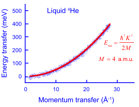
Figure 2: Schematic representation of measured dynamic structure factor $S(K,E)$ of liquid helium [47]. The red line is the calculated recoil parabola, Eq. (13), for the mass of ⁴He, shown as a guide to the eye. The white-blue ribbon around the recoil parabola represent data points measured with the time-of-flight spectrometer ARCS [48] (Adapted from [47, Fig. 1].)

Now consider the formal structure of the Doppler-term

$$E_{\textrm{Doppler}}=\frac{\hbar{\mathbf{K}\cdot\mathbf{P}}}{M}\equiv\frac{\hbar KP_{\|}}{M},$$ (15)

where $P_{\|}$ is the component of the atomic momentum parallel to K. For isotropic systems (gases, liquids, amorphous solids) the specific direction determined by K becomes immaterial, and thus $P_{\|}$ means the projection along any direction.

4.1.2 On basic theory – Scattering interaction and dynamic structure factor

The basic quantity to be experimentally determined in a neutron scattering experiment is the partial differential cross-section [40]

$$\frac{d^{2}\sigma_{M}}{d\Omega d\omega}=\frac{k_{1}}{k_{0}}b_{M}^{2}S(\textbf{K},\omega),$$ (16)

which is proportional to the measured intensity $I(\textbf{K},\omega)$. $E=\hbar\omega$, and $S(\textbf{K},\omega)$ is the dynamic structure factor of the scattering system [40]. Note that its dependence on momentum transfer $\hbar\textbf{K}$ (rather than on initial and final momenta) is a specific feature of the first Born approximation; $b_{M}$ is the so-called scattering length, i.e. a nucleus-depending constant ($M$ indicating the nucleus as well as its mass) appearing in the empirically introduced Fermi pseudo-potential

$$V_{M}(r)=\frac{2\pi\hbar^{2}}{m}b_{M}\delta(r)$$ (17)

with $r$ being the relative distance between the two colliding particles.

As already pointed out in textbooks, the standard (or conventional) theory of neutron scattering is based on Fermi’s golden rule which is equivalent to the first Born approximation; both are based on the formalism of first-order perturbation theory (see e.g [40, p. 16]). Moreover, it should be pointed out that, in principle, this theory is inapplicable to scattering by the singular potential (17); the Fermi pseudo-potential is a formal artifice defined to reproduce, in the first Born approximation, what we know to be the correct behavior for simple $s$-wave scattering (cf. [41, p. 11]).

Consider a scattering system consisting of $N$ (identical, for simplicity) atoms. The dynamic structure factor fulfills the relation

$$S({\mathbf{K}},\omega)=\frac{1}{2\pi}\int_{-\infty}^{\infty}e^{-\imath\omega\,t}F({\mathbf{K}},t)\,dt,$$ (18)

where $F({\mathbf{K}},t)$ is the so-called intermediate correlation function given by

$$F({\mathbf{K}},t)=\frac{1}{N}\sum_{j,k}^{N}\left\langle e^{-\imath{\mathbf{K}}\cdot\hat{{\mathbf{r}}}_{j}(0)}e^{\imath{\mathbf{K}}\cdot\hat{{\mathbf{r}}}_{k}(t)}\right\rangle$$ (19)

with $\langle\ldots\rangle$ denoting a thermodynamic average [40]. This function contains the Heisenberg operators

$$\hat{{\mathbf{r}}}(t)=\hat{U}^{\dagger}(t)\hat{{\mathbf{r}}}\hat{U}(t),$$ (20)

where $\hat{U}(t)$ is the unitary time evolution operator

$$\hat{U}(t)=e^{-\frac{\imath}{\hbar}\hat{H}_{c}t}$$ (21)

with $\hat{H}_{c}$ being the Hamiltonian of the complete $N$-body scattering system—not only of a single atom [40, 41].

In the limit of sufficiently large momentum transfers holds the incoherent approximation, in which terms with $j\neq k$ are neglected

$$F({\mathbf{K}},t)=\left\langle e^{-\imath{\mathbf{K}}\cdot\hat{{\mathbf{r}}}_{j}(0)}e^{\imath{\mathbf{K}}\cdot\hat{{\mathbf{r}}}_{j}(t)}\right\rangle.$$ (22)

Neutron-proton scattering is mainly incoherent also for small $K$, due to the spin-flip mechanism described by Feynman [1], as mentioned in the Introduction.

The following point should be emphasized. Quantum correlations—or even entanglement and/or quantum discord—between neutron and a scattering particle are absent in the whole conventional theory of neutron scattering; see e.g. the textbook [40] and the review article [42]. Moreover, the notion of coherence length of the neutron plays no role in conventional neutron scattering theory. (Surely, this is not the case in neutron interferometry.) This is essentially the consequence of the first-order perturbation theoretical frame of conventional theory.

4.1.3 On impulsive scattering – Impulse approximation

The key approximation called impulse approximation [42], applied in the so-called neutron Compton scattering regime, is the assumption that the collisional time $\tau$ of a neutron with a nucleus is very short. Thus the atomic (nuclear) position $r_{M}(t)$ of an atom with mass $M$ can be replaced by

$${\mathbf{r}}_{M}(t)={\mathbf{r}}_{M}(0)+t\frac{{\mathbf{P}}(0)}{M},$$ (23)

where ${\mathbf{P}}(0)$ is the initial atomic momentum. This approximation assumes that the particle travels freely over short enough times $0\leq t\leq\tau$, and thus that its interaction with other particles can be neglected.

In other words, it is assumed that the scattering particle recoils freely from the collision, with interparticle interaction in the final state being negligible and the wave function of the particle in its final state being a plane wave [42, 44].

In a real experiment, the characteristic time $\tau$ for this collision is extremely short, $\tau\rightarrow 0$, since the neutron-nucleus potential $V_{M}$ is essentially a delta function, Eq. (17). An expression for the scattering time in the impulse approximation is given by Sears,

$$\tau=\frac{M}{K\Delta P},$$ (24)

where $\Delta P$ is the width of the momentum distribution of the struck atom [42, 44]. Depending on the specific experimental parameters (and mass of scattering atom), $\tau$ lies roughly in the femtosecond, or attosecond, time range [42, 43, 44].

In the context of weak measurement and two-state-vector formalism, it is important to observe that the basic Eqs. (18,19) depend on dynamical variables of the scattering system only [40]) and no dynamical variable of the neutron—e.g. the parameter $b_{M}$ is not a dynamical variable but a c-number.

In the limit of sufficiently large momentum transfer, i.e. in the impulse approximation, conventional theory yields for the dynamic structure factor the simple expression [42, 43, 44]

$$S_{M}({\mathbf{K}},\omega)=\left\langle\delta\left(\hbar\omega-\hbar\omega_{\textrm{rec}}-\frac{\hbar{\mathbf{K}}\cdot{\mathbf{P}}}{M}\right)\right\rangle\ \ \ \ \ \ \ \ \ \ \ \ \ \ \ \ \$$

$$\ \ \ \ \ \ \ \ \ \ \ \ \ =\int\!n_{M}({\mathbf{P}})\,\delta\left(\hbar\omega-\hbar\omega_{\textrm{rec}}-\frac{\hbar{\mathbf{K}\cdot\mathbf{P}}}{M}\right)dP,$$ (25)

where $n({\mathbf{P}})$ is the classical distribution function of the atomic momenta in the initial state and the delta function represents the aforementioned energy conservation (12). As the scatterer is initially at rest, it holds $\langle P\rangle=0$.

For the case of one atom with momentum-space wave function $\Xi(P)$ (i.e. the Fourier transform of the wave function $\Psi(r)$ in position space), this is given by [42, 43, 44]

$$n_{M}(P)=|\Xi(P)|^{2}.$$ (26)

This formula physically means that here the measured signal (intensity, dynamical structure factor) contains an incoherent sum (superposition) over the classical probability distribution of initial-state momenta—and not a coherent superposition of the scattering amplitudes before taking the absolute square. In other terms, this expression contains only the diagonal part of the full density operator $|\Xi\rangle\langle\Xi|$, i.e. all non-diagonal terms are discarded. Also this weakness is a consequence of the first-order perturbation theory underlying the impulse approximation of conventional theory.

A remarkably concise derivation of the main result, Eq. (25), including a short explanation of incoherent and impulse approximations, is given by Sears in the first three pages of [44].

4.2 Conventional final-state effects, peak shift, and effective mass

In real experiments, deviations from the impulse approximation may be observed. Here, we will consider them within the frame of conventional theory.

The aforementioned energy conservation relation (12) for a two-body collision holds exactly in the impulse approximation, but is not completely fulfilled at momentum and energy transfers of actual experiments, in which so-called final-state effects may become apparent. (In fact, this term commonly includes both initial and final state effects; see [42, 44] and papers cited therein.) These are caused by environmental forces on the struck particle, which affect both initial and final states of it. Here, we will shortly discuss this effect in the frame of conventional theory.

If the scatterer is not completely free but partially bound to other particles of its environment, then the probe particle scatters on an object with higher effective mass, as the particles of the environment have a certain mass; in other terms, the scattering particle becomes hindered by the environmental forces. The latter may be due to some conventional mechanism of binding (such as ionic or van der Waals forces; chemi- or physisorbtion). However these forces can never cause an increase of the particle’s mobility, or equivalently, a reduction of its effective mass. The particle is dressed by certain environmental degrees of freedom, which is tantamount to a small increase of its effective mass,

$$M_{\textrm{eff}}\geq M_{\textrm{free}}\equiv M.$$ (27)

The above remarks correspond to a well understood effect, often observed in scattering from condensed systems; cf. [42, 43, 44].

These illustrative considerations imply that relation (27) should be valid also in the final state of the struck particle. Moreover, it should hold under the conditions of neutron Compton scattering as well as of incoherent inelastic neuron scattering.

This effect can be also shown by referring to the aforementioned energy conservation relation, see (14), here including a small term $E_{\textrm{int}}>0$ describing the atom-environment interaction:

$$\bar{E}=\frac{\hbar^{2}\bar{K}^{2}}{2M}+E_{\textrm{int}},$$ (28)

where $\bar{E}$ and $\bar{K}$ refer to the center of a measured peak (with one detector). Note that these quantities are determined from the kinematics of the neutron, in contrast to $E_{\textrm{int}}$ which is a quantity of the scattering system. Let us now try to fulfill this equation with a pair $(E_{\textrm{IA}},K_{\textrm{IA}})$ being determined by the impulse approximation for which holds $E_{\textrm{IA}}=\hbar^{2}K_{\textrm{IA}}^{2}/2M$. Then Eq. (28) yields

$$E_{\textrm{IA}}=\frac{\hbar^{2}K_{\textrm{IA}}^{2}}{2M_{\textrm{eff}}}+E_{\textrm{int}},$$ (29)

where $E_{\textrm{int}}>0$ necessarily implies $M_{\textrm{eff}}>M$.

From the considered increase of effective mass, $M_{\textrm{eff}}>M$, and Eq. (29) one obtains the following experimentally testable predictions of conventional theory:

$(a)$ Assuming $K$-transfer to be fixed in a specifically designed experiment—a so-called constant-$K$ measurement—the recoil (i.e. kinetic) energy of an atom with mass $M_{\textrm{eff}}$ will be smaller than predicted by the impulse approximation (in which the atom is free and has mass $M$). An example is given in Fig. 2 of [42], which demonstrates this effect with the aid of an exact calculation of scattering from a harmonic oscillator. The envelope of the exact transition lines is shifted to a lower energy than that of the calculated impulse approximation line; this shift corresponds to the recoil of a fictitious free particle with a larger effective mass than that of the oscillator.

$(b)$ Assuming $E$-transfer to be fixed in a specifically designed experiment—a so-called constant-$E$ measurement—the momentum transfer to a recoiling atom with mass $M_{\textrm{eff}}$ will be larger than predicted by the impulse approximation (in which the atom is free and has mass $M$).

It may be noted that various generalizations of the impulse approximation, including initial and final-state effects, predict similar results. For example, Stringari’s well-known model [49] predicts a shift of the measured recoil peak to lower $E$-transfer, in accordance with case $(a)$. Furthermore, this shift was demonstrated with deep-inelastic neutron scattering data from liquid helium at $K=10\,\AA^{-1}$ [49].

Summarizing, conventional theory cannot predict a decrease of the scatterer’s effective mass—and/or associated deviations of $E$- and $K$-transfers—opposite to those of cases $(a)$ and $(b)$ .

4.3 Neutron scattering – Weak interaction

As general (non-relativistic) scattering theory [50] shows, scattering of an incoming neutron wave packet $\psi_{n}$ from a particle in the state $\psi_{A}$ is described by

$$\psi_{n}\psi_{A}\rightarrow(\psi_{n}\psi_{A})_{\textrm{unscatt}}+\varepsilon\Psi(n,A)_{\textrm{scatt}}$$ (30)

(up to normalization; $|\varepsilon|\ll 1$) where the two subscripts denote the non-scattered and scattered components. This process is represented by an ordinary unitary transformation. In the center-of-mass coordinate system, the scattered component is given by an outgoing spherical wave (which is called $s$-wave scattering). In particular, for neutron scattering it holds

$$\varepsilon\Psi(n,A)_{\textrm{scatt}}\propto-\frac{b_{M}}{r}\exp(\imath kr),$$ (31)

where $r$ denotes the relative spatial distance between the two particles, ${b_{M}}$ is the scattering length of the atomic nucleus with mass $M$, and $k$ a proper wave vector. For the (arbitrary) choice of the minus sign in this expression, see [40].

The range of the nuclear forces is very short (of the order of $10^{-15}$ m = 1 fm), and the associated scattering length $b_{M}$ in the Fermi pseudo-potential, Eq. (17), is of similar order, say 1–10 fm. Due to the much larger de Broglie wavelength of the impinging neutrons (being of the order of 1 Åfor thermal neurons), the scattering contains only $s$-wave components [40, 41].

Note that usually the struck nucleus (atom) is not fully fixed and thus exhibits some recoil, which is particularly significant for a struck H-atom. Hence neutron and scattering particle are entangled in their two-body final state.

Due to the smallness of scattering lengths of all nuclei [40] and the associated ultrashort range of the nuclear forces, the neutron-nucleus scattering (commonly referred to as neutron-atom scattering) represents a weak interaction, and for this reason the theoretical framework of first-order perturbation theory is assumed to be fully sufficient. In this context, it should be reminded that the general van Hove formalism of time-correlation functions [51], on which every conventional neutron scattering theory is based (cf. textbooks [40, 41]), contains time-dependent (Heisenberg) operators of the undisturbed $N$-body scattering system only—i.e. the disturbance caused by the neutron-system interaction is assumed infinitesimally weak.

For further insight on how weak the neutron-atom interaction is, the following fact may be noted. Every existing neutron beam (e.g. at the newest and most intense spallation source SNS) is weak also in the sense that the probability for two neutrons of a neutron pulse to scatter off the same atom is practically zero.

However, in the theoretical frame of weak values and two-state-vector formalism, the weakness of interactions should be examined in some more detail. To yield a numerical estimate, we take into account the discussion by Duck, Stevenson and Sudarshan [17]. These authors pointed out that the weak value theoretical derivations of [15] require (among other conditions) that the state of the weak measuring device must be representable by a wave function, rather than by an impure density matrix. This can be achieved with the probe beam being coherent across its width.

In the neutron scattering experiments considered below (in Section 6), the neutron’s coherence width is not specified in the cited references. This is because this quantity plays no role in conventional neutron scattering theory. To determine this quantity, details of the beam’s monochromaticity and divergence would be needed. In order to proceed, and as a rough estimate of the worst case, here we may assume this coherence width to be similar to, or larger than, the neutron’s wavelength $\lambda_{n}$. Thus the magnitude of the total scattering amplitude of the neutron wave from a nucleus, which should be proportional to $b_{M}$, can be roughly estimated by the ratio

$$\varepsilon\lesssim\frac{b_{M}}{\lambda_{n}}\sim\frac{10\ \textrm{fm}}{1\ \textrm{\AA}}=10^{-4}.$$ (32)

Depending on details of the instrumental setup, usually the neutron-beam coherence width in real experiments should be larger than the neutron wavelength. (It may be noted that in various experimental setups of neutron interferometry, this coherence width can be of the order of 1 cm.)

This crude estimate shows that the non-relativistic scattering of neutrons at issue can be safely considered as a weak interaction process. Due to the smallness of the interaction range and the ultrashort collisional time, the process is impulsive.

5 Elementary scattering in the light of weak measurement and two-state-vector formalism

5.1 On shift operator and momentum transfer in impulsive two-body collisions (conventional theory)

In this section, the position and momentum of the neutron (probe particle) are denoted as $(q,p)$. Similarly, the position and momentum of the scatterer (atom, nucleus) are denoted as $(Q,P)$. A symbol, say $X$, with a hat, $\hat{X}$, represents the corresponding operator quantity. To illustrate the action of shift operators, let us consider here a simple one-dimensional quantum model for momentum exchange in a two-particle impulsive collision.

Let us furthermore assume that the two particles occupy states with approximately well defined momenta (i.e. plane waves). The initial state of the whole system is usually assumed to be uncorrelated:

$$\Psi_{\textrm{initial}}=\phi_{n}(p)\otimes\Xi_{A}(P)$$ (33)

(indices $n$ and $A$ refer to neutron and atom, respectively).

An impulsive scattering process may be formally described by the (oversimplified) interaction Hamiltonian

$$\hat{V}=F(t)\,(\hat{q}-\hat{Q}),$$ (34)

where the function $F(t)$ represents a non-zero force during a short time interval $\tau$, i.e. the duration of the collision; e.g. we may assume that $F(t)$ is proportional to a delta function. Furthermore it is assumed that the integral over $F(t)$

$$\int_{0}^{\tau}F(t)\,dt=\hbar K$$ (35)

gives the momentum transfer $\hbar K$ caused by the collision.

Neutron and atom observables commute, so $[\hat{q},\hat{Q}]=0$, and the associated unitary evolution operator is

$$\hat{U}(\tau)=e^{-(\imath/\hbar)\int\hat{V}dt}=e^{-(\imath/\hbar)\,\hbar K\,(\hat{q}-\hat{Q})}\equiv e^{-\imath\,K\,\hat{q}}e^{+\imath\,K\,\hat{Q}}.$$ (36)

The operator $e^{\imath\hbar K\,\hat{Q}/\hbar}$ shifts an atomic momentum eigenket as $e^{\imath\hbar K\,\hat{Q}/\hbar}|P\rangle=|P+\hbar K\rangle$ while the operator $e^{-\imath\hbar K\,\hat{q}/\hbar}$ shifts an impinging particle (neutron) momentum eigenket as $e^{-\imath\hbar K\hat{q}/\hbar}|p\rangle=|p-\hbar K\rangle$.

Immediately after the momentum exchange, the state of the two-particle system in the momentum representation is

$$\Psi_{\textrm{final}} = \hat{U}(\tau)\,\phi_{n}(p)\otimes\Xi_{A}(P)$$ (37)

$$= e^{-i\hbar K\,\hat{q}/\hbar}\phi_{n}(p)\otimes e^{i\hbar K\,\hat{Q}/\hbar}\Xi_{A}(P)$$

$$= \phi_{n}(p+\hbar K)\otimes\Xi_{A}(P-\hbar K).$$

This final state is not entangled, due to the trivial form of $\hat{V}$. These short considerations may motivate the search for a two-body impulsive interaction Hamiltonian, which is presented in the following section.

Concerning the basic importance of the shift operator in demonstrating the dynamical non-locality of quantum mechanics, see the discussion by Popescu [52].

5.2 Weak measurement, interaction Hamiltonian and momentum transfer

As already mentioned in connection with Eq. (15), for our purposes it is sufficient to consider the atomic momentum component parallel to K, which from now on we shall denote simply by $P$—and the associated operator by $\hat{P}$. In other words, in the following calculations we shall consider the dynamics along an arbitrarily chosen direction of momentum transfer, which is an one-dimensional problem.

5.2.1 Von Neumann-type interaction Hamiltonian

In this subsection, we provide a physically motivated heuristic derivation of a von Neumann-type interaction Hamiltonian for (a given amount of) momentum transfer in an impulsive collision.

Let us start again with the one-body model Hamiltonian describing momentum transfer $-\hbar K\equiv+\hbar K_{n}$ on the neutron due to the collision with the atom:

$$\hat{V}_{n}(t)=\delta(t)\,\hbar K\,\hat{q}.$$ (38)

As shown above, the associated evolution operator acting on the space of the neutron

$$\hat{U}_{n}(\tau)=e^{-\frac{\imath}{\hbar}\,\hbar K\,\hat{q}}$$ (39)

shifts a momentum eigenstate of the impinging particle (neutron) as $e^{-\imath\hbar K\hat{q}/\hbar}|p\rangle=|p-\hbar K\rangle$.

Assuming momentum conservation in the two-body collision, it holds

$$-\hbar K_{n}=\hbar K_{A}\equiv\hbar K,$$ (40)

where $\hbar K_{A}$ is the momentum transfer on the atom due to the collision. (We choose $K_{A}$ with positive sign, following standard notation of conventional theory [40, 41].)

The scattering atom is assumed at rest in its initial state before collision, $\langle\hat{P}\rangle_{i}=0$. After the collision, one conventionally expects that

$$\hbar K_{A}=+\hbar K=\langle\hat{P}\rangle_{f}=\langle\hat{P}\rangle_{f}-\langle\hat{P}\rangle_{i}$$ (41)

and correspondingly for the neutron momentum

$$\hbar K_{n}=-\hbar K=\langle\hat{p}\rangle_{f}-\langle\hat{p}\rangle_{i}.$$ (42)

Hence, the aforementioned operator $\hat{U}_{n}(\tau)$ of the neutron, Eq. (39), may be written as

$$\hat{U}_{n}(\tau)=e^{-\frac{\imath}{\hbar}\,\langle\hat{P}\rangle_{f}\,\hat{q}}.$$ (43)

To apply the theory of weak measurement and two-state-vector formalism, a von Neumann two-body interaction Hamiltonian is needed. Thus one is intuitively guided to try a two-body generalization of the one-body evolution operator $\hat{U}_{n}(\tau)$ of the form

$$\hat{U}(\tau)=e^{-\frac{\imath}{\hbar}\,\hat{q}\,\hat{P}}.$$ (44)

This heuristically obtained expression still has not obvious context to the real experimental situations under consideration. To achieve this, we now may proceed as follows.

Firstly, let us refer to the aforementioned impulse approximation and Eq. (12) regarding energy conservation:

$$E=\frac{(\hbar K)^{2}}{2M}+\frac{\hbar{\mathbf{K}\cdot\mathbf{P}}}{M}.$$

Looking at this equation, one sees that the larger recoil term $\frac{(\hbar K)^{2}}{2M}$ may be viewed to result from a strong impulsive interaction (associated with momentum transfer $+\hbar K$ on the atom). The theoretical treatment of this part of the interaction is not within the scope of the present paper. Since in the impulse approximation usually holds $|K|\gg|P|$, the smaller Doppler term $\frac{\hbar{\mathbf{K}\cdot\mathbf{P}}}{M}$ may correspond to a weaker interaction, in which the atomic momentum $\hat{P}$ couples with an appropriate dynamical variable of the neutron, say ${\cal{\hat{O}}}_{n}$. Looking at the preceding formulas (43,44) for the model operator effectuating momentum transfer, it appears that this dynamical variable should be $\hat{q}$, that is ${\cal{\hat{O}}}_{n}=\hat{q}$ .

Secondly, in view of the theory of weak values and two-sate-vector formalism, the weak interaction is expected to cause weak deviations from (or: additional small contributions to) the conventionally expected large momentum transfer $\hbar K$. This can be introduced into the formalism by replacing $\hat{P}$ with the small momentum difference $\hat{P}-\hbar K\hat{I}_{A}$, and also including a positive smallness factor

$$0<\lambda\ll 1$$

in the model interaction Hamiltonian and the associated evolution operator. In particular, let us assume the model interaction Hamiltonian

$$\hat{H}_{\textrm{int}}(t)=+\lambda\,\delta(t)\,\hat{q}\otimes(\hat{P}-\hbar K\,\hat{I}_{A}).$$ (45)

It may be noticed that this model Hamiltonian is not put forward entirely on kinematical grounds, like Eq. (40), but also on quantum dynamical grounds, e.g. the choice ${\cal{\hat{O}}}_{n}=\hat{q}$ of the canonically conjugate operator $\hat{q}$ to neutron’s momentum $\hat{p}$.

Moreover, it should be pointed out that the plus sign in front of this expression is not arbitrary, since it is consistent with the definitions (40). This point will be addressed explicitly in subsection 5.3.1, since it plays a decisive role in the context of the new quantum effect of momentum transfer deficit.

For further physical motivation of the two parts of the model Hamiltonian of Eq. (45), it may be helpfully to compare the above reasoning with an example by Aharonov et al.:

Consider, for example, an ensemble of electrons hitting a nucleus in a particle collider. $\left[\ldots\right]$ The main interaction is purely electromagnetic, but there is also a relativistic and spin-orbit correction in higher orders which can be manifested now in the form of a weak interaction. [53, p. 3]

5.2.2 Weak value of atomic momentum operator $\hat{P}$

Let consider the atom as the system. Since the weak value of the identity operator is $(\hat{I}_{A})_{w}=1$, for the weak value of the atomic coupling operator $\hat{P}-\hbar K\,\hat{I}_{A}$ in the above interaction Hamiltonian holds:

$$(\hat{P}-\hbar K\,\hat{I}_{A})_{w}=P_{w}-\hbar K.$$ (46)

In the following, we first calculate the weak value $P_{w}$ of $\hat{P}$ for some characteristic (and experimentally relevant) final states in momentum space. The results will reveal a striking deviation—more precisely, a deficit—from the conventionally expected momentum transfer to the neutron; to the latter belongs the pointer momentum variable $\hat{p}$ conjugated to $\hat{q}$ appearing in Eq. (45).

For the calculation of the weak value, it seems natural to use the momentum space representation, as scattering experiments usually measure momenta (rather than the positions of the scatterers in real space).

Let the atom initially be at rest and in a spatially confined state (e.g. in a potential representing physisorption on a surface; cf. experiments in Section 6). Then the initial atomic wave function $\Xi(P)_{i}$ can often be approximated by a Gaussian $G_{A}$ centered at zero momentum,

$$\Xi(P)_{i}\approx G_{A}(P).$$

At sufficiently deep temperature the atom will be in its ground state, and the width of $\Xi(P)_{i}$ is determined by the quantum uncertainty.

The struck atom moves in the direction of momentum transfer $\hbar K_{A}=\hbar K$; therefore, to simplify notations, in the following calculations $P$ represents the atomic momentum along the momentum transfer direction.

It will be instructive to consider the following three cases for the atomic final state:

$(A)$ The final state is a plane wave (has vanishing width in momentum space)—as assumed in general conventional theory and the impulse approximation. Here, the result of conventional theory is reproduced.

$(B)$ The final state has a small but non-vanishing width in momentum space.

$(C)$ Initial and final states have the same width in momentum space.

$(A)$ Plane wave as final state. As in the case of the usual impulse approximation [42] of Compton scattering from a single scatterer, let the final state be a plane wave; that is the momentum wave function is a delta function $\delta_{A}$ centered at the assumed transferred momentum $\hbar K_{A}$,

$$\Xi(P)_{f}=\delta_{A}(P-\hbar K_{A}).$$ (47)

The weak value of $\hat{P}$ follows straightforward:

$$P_{w} = \frac{\langle\Xi_{f}|\hat{P}|\Xi_{i}\rangle}{\langle\Xi_{f}|\Xi_{i}\rangle}$$ (48)

$$= \frac{\int dP\,\delta_{A}(P-\hbar K_{A})\,P\,\Xi(P)_{i}}{\int dP\,\delta_{A}(P-\hbar K_{A})\,\Xi(P)_{i}}$$

$$= \frac{\hbar K_{A}\,\Xi(\hbar K_{A})_{i}}{\Xi(\hbar K_{A})_{i}}$$

$$= +\hbar K_{A}\equiv+\hbar K.$$

(Recall the notations of Eq. (40).) Hence, the weak value of the system coupling operator $(\hat{P}-\hbar K\,\hat{I}_{A})$ is just zero,

$$(\hat{P}-\hbar K\,\hat{I}_{A})_{w}=P_{w}-\hbar K=0.$$ (49)

(According to standard quantum scattering theory, the scattered wave may acquire an additional phase factor, say $e^{\imath\chi}$, which does not affect the preceding result because this factor cancels out in the fractions of Eqs. (48).)

This physically means that, in this case, the new theory yields no correction to the conventionally expected value of momentum transfer (i.e. $-\hbar K$, by assumption) shown by the pointer of the measuring device, namely:

$$\langle\hat{p}\rangle_{f}-\langle\hat{p}\rangle_{i}=-\lambda\,(\hat{P}-\hbar K\,\hat{I}_{A})_{w}=0.$$ (50)

Thus, the result of Eq. (49) is consistent with conventional theory of the impulse approximation (or, more generally, of incoherent neutron scattering); cf. also Eq. (37).

$(B)$ Final state with non-vanishing width. Relaxing and generalizing the strict impulse approximation assumption of case (A), let us make here the more realistic assumption that the atomic final state is represented by a widened delta-like symmetric function $\Delta_{A}$ with finite (small) width, which is centered again at the conventionally expected momentum transfer $\hbar K_{A}$. That is,

$$\Xi(P)_{f}=\Delta_{A}(P-\hbar K_{A})$$ (51)

for which holds again $\langle\Xi_{f}|\hat{P}|\Xi_{f}\rangle=\hbar K_{A}$. For example, a Gaussian with (much) smaller width than the initial state fulfils these conditions. The weak value of the atomic momentum operator is then

$$P_{w} = \frac{\langle\Xi_{f}|\hat{P}|\Xi_{i}\rangle}{\langle\Xi_{f}|\Xi_{i}\rangle}$$ (52)

$$= \frac{\int dP\,\Delta_{A}(P-\hbar K_{A})\,P\,\Xi(P)_{i}}{\int dP\,\Delta_{A}(P-\hbar K_{A})\,\Xi(P)_{i}}$$

$$= +\hbar K_{A}-\pi(\hbar K_{A})$$

$$\equiv +\hbar K-\pi(\hbar K_{A}),$$

where the small momentum correction $\pi(\hbar K_{A})$ fulfills

$$0<\pi(\hbar K_{A}).$$ (53)

This can be easily seen as follows. In the nominator

$$\int dP\,\Delta_{A}(P-\hbar K_{A})\,P\,\Xi(P)_{i}$$

the factor $\Xi(P)_{i}$ gives more weight to the left side (i.e. for $P<\hbar K_{A}$) of the symmetric peak $\Delta_{A}(P-\hbar K_{A})$ than to the right side; this leads to an average of $P$ being smaller than the central position $\hbar K_{A}$ of the final state $\Delta_{A}$.

Obviously, the correction term $\pi(\hbar K_{A})$ vanishes in the plane wave (and also the impulse) approximation limit, as already considered in the preceding case $(A)$; i.e.

$$\Delta_{A}\rightarrow\delta_{A}\ \ \Rightarrow\ \ \pi(\hbar K_{A})\rightarrow 0.$$

Furthermore, we see that the finite width of the final state causes a reduction of the conventionally expected momentum transfer $\hbar K$; namely

$$(\hat{P}-\hbar K\,\hat{I}_{A})_{w}=P_{w}-\hbar K=-\pi(\hbar K_{A})$$ (54)

and consequently for the additional shift of the meter pointer variable holds

$$\langle\hat{p}\rangle_{f}-\langle\hat{p}\rangle_{i} = -\lambda\,(\hat{P}-\hbar K\,\hat{I}_{A})_{w}$$ (55)

$$= +\lambda\,\pi(\hbar K_{A}).$$

Here, we made use of the general result given by Eq. (3); see also Eq. (59).

$(C)$ Final state with unchanged width. The collisional process is here assumed to be soft enough in order to leave the shape of the initial state unchanged. In other words, let the final state have the same shape as the initial state, but be centered at the transferred momentum; i.e.

$$\Xi(P)_{f}=\Xi(P-\hbar K_{A})_{i}.$$ (56)

The weak value of the atomic momentum operator is now as follows:

$$P_{w} = \frac{\langle\Xi_{f}|\hat{P}|\Xi_{i}\rangle}{\langle\Xi_{f}|\Xi_{i}\rangle}$$ (57)

$$= \frac{\int dP\,\Xi(P-\hbar K_{A})_{i}\,P\,\Xi(P)_{i}}{\int dP\,\Xi(P-\hbar K_{A})_{i}\,\Xi(P)_{i}}$$

$$= +\frac{\hbar K_{A}}{2}=+\frac{\hbar K}{2}.$$

The last equality follows immediately from $(a)$ the two symmetrically distributed $\Xi$ functions around their central position $\bar{P}=\hbar K_{A}/2$ and $(b)$ the linear term $P$ in the integral of the nominator. It should be noted that this result does not depend on the width of $\Xi$, as long as the two $\Xi$ functions are not orthogonal to each other.

In other words, the correction term of the momentum transfer is here $\pi(\hbar K_{A})=\frac{\hbar K_{A}}{2}$.

This is a quite interesting result because it represents a momentum-transfer deficit of 50%; i.e. the scattered neutron measures a momentum kick being only half of the conventionally expected value. In more detail:

$$(\hat{P}-\hbar K\,\hat{I}_{A})_{w}=+\frac{\hbar K_{A}}{2}-\hbar K=-\frac{\hbar K}{2}$$

and applying Eq. (3), or Eq. (59), one obtains for the correction to the shift of the meter pointer variable:

$$\langle\hat{p}\rangle_{f}-\langle\hat{p}\rangle_{i}=-\lambda\,(\hat{P}-\hbar K\,\hat{I}_{A})_{w}=+\lambda\,\frac{\hbar K}{2}.$$ (58)

In subsection 6.2, we will present and discuss a recent striking experimental finding being qualitatively comparable with this numerical result.

The rather general scheme of the above derivations provides evidence that the new effect under consideration is not a specific feature of the simple time-of-flight experiment at issue, but a general one of any field of scattering physics, e.g. relativistic scattering in high-energy physics. The immediate implication is that the general theory of weak measurement and two-state-vector formalism may be relevant for a very broad range of modern scattering experiments.

5.3 Quantum momentum-transfer deficit

As the above calculations show, in all cases under consideration the weak value $P_{w}$ is real. Hence for the calculation of the expectation value of the meter output variable $\hat{p}$, which is the neutron’s momentum (conjugate to $\hat{q}$), the general result of Eq. (3) applies. Here, it should be noted the change of sign between the usually applied interaction Hamiltonian of Eq. (2), as e.g. treated in [15, 17], and the presently used specific form (45). Therefore, there is a corresponding change of sign in the result of Eq. (3), namely

$$\langle\hat{p}\rangle_{f}-\langle\hat{p}\rangle_{i}=-g\,\textrm{Re}[A_{w}].$$ (59)

The preceding results of Eqs. (52) and (57) imply that the meter variable $\hat{p}$ will not take the conventionally expected value $-\hbar K=-\hbar K_{A}$, but an anomalous value due to the reduction term $\lambda\,(\hat{P}-\hbar K\,\hat{I}_{A})_{w}=-\lambda\,\pi(\hbar K_{A})$. In particular, for the total momentum transfer shown by the pointer momentum we may write:

$$\left[\langle\hat{p}\rangle_{f}-\langle\hat{p}\rangle_{i}\right]_{\textrm{total}}\ \ = \left[\langle\hat{p}\rangle_{f}-\langle\hat{p}\rangle_{i}\right]_{\textrm{conventional}}$$ (60)

$$\ \ \ \ \ \ \ +\left[\langle\hat{p}\rangle_{f}-\langle\hat{p}\rangle_{i}\right]_{\textrm{correction}}$$

$$= -\hbar K+\lambda\,\pi(\hbar K_{A}).\ \$$

This result represents the new quantum effect of quantum momentum-transfer deficit: the absolute value of momentum transfer on the neutron predicted by the new theory is smaller than that predicted by conventional theory; in short,

$$|-\hbar K+\lambda\,\pi(\hbar K_{A})|\leq|-\hbar K|.$$

The weak measurement result (60) has some conceptual similarity with the result by Aharonov et al. discussed in Section 3, in which the interferometer mirror received momentum kicks only from the insight, but the strange result was that these kicks (under the proper post-selection) somehow succeed to pull it in instead to push it out [38].

As mentioned above, the physical reason of this new effect is the specific quantum interference being revealed by the theory at issue, which is associated with the post selection. As far as we know, this effect has no explanation within the frame of conventional theory of scattering. Moreover, it is in blatant contradiction with conventional expectations of neutron scattering theory even qualitatively, as discussed in subsection 4.2.

5.3.1 The positive sign of the model interaction Hamiltonian

It was pointed out above that the plus sign in front of model interaction Hamiltonian $\hat{H}_{\textrm{int}}$ in Eq. (45) is necessary and not due to an arbitrary choice; see subsection 5.2.1. This positive sign is critical to the presented conclusions.

However, one might object this point and claim the following: If one replaces $+\lambda$ with a negative factor, say $-\mu$ (where $\mu>0$), in the Hamiltonian (45), one may carry through the above derivations to arrive at a positive momentum transfer correction without any violation of momentum conservation.

Here, we will show that this objection is incorrect. First, the calculations of weak value $(\hat{P}-\hbar K\,\hat{I}_{A})_{w}=-\pi(\hbar K_{A})$ remain unaffected, since the operator does not contain the factor $\lambda$. Second, the replacement of the positive factor $+\lambda$ with the negative factor $-\mu$, yields the new Hamiltonian

$$\hat{H}_{\textrm{int,new}}(t)=-\mu\,\delta(t)\,\hat{q}\otimes(\hat{P}-\hbar K\,\hat{I}_{A})$$ (61)

and, at the same time, causes a change of the sign of the general theoretical result (59), which for the specific correction to the pointer shift (59) under consideration reads

$$\langle\hat{p}\rangle_{f}-\langle\hat{p}\rangle_{i} = +\mu\,(\hat{P}-\hbar K\,\hat{I}_{A})_{w}$$ (62)

$$= -\mu\,\pi(\hbar K_{A}).$$

In particular, the correction term to the pointer momentum shift is now negative. This increases the absolute value of the total shift:

$$|-\hbar K-\mu\,\pi(\hbar K_{A})|\geq|-\hbar K|$$

and, therefore, this increase is qualitatively in contrast to the decreased weak value of atomic momentum

$$(\hat{P})_{w}=+\hbar K_{A}-\pi(\hbar K_{A}).$$

(Recall that $\hbar K_{A}=\hbar K$, by definition.)

In simpler terms, using the new interaction Hamiltonian (61) we arrive at an unphysical result: The weak value of the atomic momentum transfer is still reduced (with respect to conventional theory), but the measuring apparatus shows an increased momentum transfer. Obviously, this unphysical paradox is an artifact of the wrongly chosen negative sign in the model Hamiltonian Eq. (61)—and not a weakness of the general theory of weak values and two-state-vector formalism. Namely, this paradox vanishes if the correct (i.e. physically appropriate) model Hamiltonian of Eq. (45) is applied.

Contradicting the above explanations, one might insist that the choice of the negative factor $-\mu$ in the model Hamiltonian (61) should be still legitimate. However, as shown, Eq. (61) implies that the measuring system (i.e. the scattered neutron) exhibits an increased momentum transfer—which is tantamount to the aforementioned (in Section 4) expectations of conventional theory, in particular the conventional final-state effects. But the recent experimental results presented in Section 6 are in blatant contrast to conventional theory.

The above considerations refer explicitly to both quantum systems (i.e. atom and neutron). This is because the model interaction Hamiltonian $\hat{H}_{\textrm{int}}$ in Eq. (45) contains dynamical variables of both systems, and therefore its physical significance cannot be discussed by considering the scattering atom (and the weak value of $\hat{P}$) only.

6 Experimental context and results

In this section, the obtained weak measurement results are compared with real experiments. The derivations of the preceding section should apply to both neutron scattering subfields of interest—neutron Compton scattering and incoherent inelastic neuron scattering—as they do not contain any specific assumption being valid in one subfield only. The presented experimental results may be considered as possible examples of the theoretical analysis of Section 5; other explanations are presently unknown, but they cannot be excluded yet.

6.1 Neutron Compton scattering from H atoms of a solid polymer

An experimental demonstration of the new quantum effect under consideration can be found in the data of [54]. The deep-inelastic neutron scattering experiments were carried out by Cowley and collaborators with the time-of-flight spectrometer MARI [55] of the neutron spallation source ISIS (Rutherford Appleton Laboratory, UK). The sample (a foil of a solid polymer) was at room temperature. Fig. 3 shows two examples of the extensive measurements reported in [54]. The depicted recoil peaks are mainly due to scattering from protons (H atoms), due to the high scattering cross-section of H. The vertical (red) lines show the $E$-transfer positions of the peaks according to conventional theory, Eq. (13). The centroids of the measured recoil peaks are markedly shifted to higher energy transfer than conventionally expected. As discussed in subsection 4.2, this shift is equivalent to a smaller effective mass of the recoiling H atom.

One might object that the shown data contain an additional small contribution from the C recoil. However this is located at smaller $E$-transfers than that of H, due to their mass difference. Therefore the above qualitative conclusion remains unaffected.

It may be noted that the shown neutron Compton scattering peaks are very broad and asymmetric, which is due to the (very) low resolution of the employed modified setup of MARI [54]. This makes a quantitative analysis to determine the peak-position impossible. Nevertheless, visual inspection of the data shows that the centroids of the peaks are shifted to higher energy roughly by 5-10 % of the recoil energy, which equivalently means that the effective mass $M_{\textrm{eff}}$ of the recoiling H atoms is smaller than $M_{\textrm{H}}=1.0079$ a.m.u. of a free H by the same percentage

$$M_{\textrm{eff}}(\textrm{H})\approx 0.91-0.96\ \ \textrm{a.m.u.}$$ (63)

It is also interesting to look at the additional (about 50) spectral data reported in [54]. Remarkably, all those peaks appeared to show always positive $E$-transfers, i.e. with no scatter to negative $E$-transfers; see [54, Fig. 12]. This underlines considerably the reliability of the $E$-shift at issue. However, since the main aim of that investigation was motivated differently (i.e. to measure the cross-section of H), this striking experimental finding remained fully unnoticed in the discussions of [54].

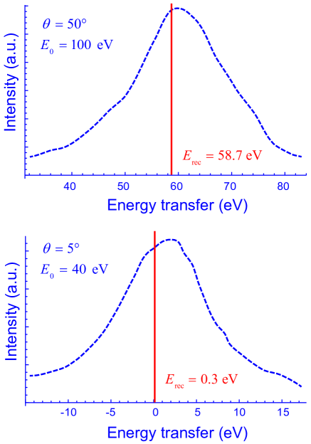
Figure 3: Schematic representation of two examples of deep-inelastic neutron scattering spectra from a solid polymer (polyethylene, $[-\textrm{CH}_{2}-]_{n}$) measured with the time-of-flight spectrometer MARI of ISIS [54]. Peak-shifts to higher energy transfers than the conventionally expected recoil energy $E_{\textrm{rec}}$ (vertical red lines) are clearly visible. This corresponds to a lower effective mass of the recoiling H; see the text. For experimental details and more examples, see [54].

Noteworthy, throughout this section we presumed that the calibration of the instrument MARI employed in the experiment [54] was correct, i.e. that the applied time-of-flight method (see subsection 4.1) used correct instrumental parameters.

6.2 Incoherent inelastic scattering from single H₂ molecules in nanopores

Another surprising result from incoherent inelastic neutron scattering was observed by Olsen et al. [56] in the quantum excitation spectrum of H₂ adsorbed in multi-walled nanoporous carbon (with pore diameter about 8–20 Å).

The incoherent inelastic neutron scattering experiments were carried out at the new generation time-of-flight spectrometer of Spallation Neutron Source SNS (Oak Ridge Nat. Lab., USA), called ARCS [48]. In this experiment, the temperature was $T=23$ K, and the incident neutron energy $E_{0}$ was 90 meV. The latter implies that the energy transfer cannot excite molecular vibrations (or break the molecular bond), but only excite rotation and translation (also called recoil) of H₂ which interacts only weakly with the substrate:

$$E=E_{\textrm{rot}}+E_{\textrm{trans}}.$$ (64)

The experimental two-dimensional incoherent inelastic neutron scattering intensity map $S(K,E)$ of H (after background subtraction) is shown in Fig. 4, which is adapted from the original paper [56]. The following features are clearly visible. First, the intensive peak centered at $E_{\textrm{rot}}\approx 14.7$ meV corresponds to the well-known first rotational excitation $J=0\rightarrow 1$ of the H₂ molecule [57]. Furthermore, the wave vector transfer of this peak is $K_{\textrm{rot}}\approx 2.7$ Å^-1. Thus the peak position in the $K$–$E$ plane shows that the experimentally determined mass of H that fulfills the relation $E_{\textrm{rot}}=(\hbar K_{\textrm{rot}})^{2}/2M_{\textrm{H}}$ is (within experimental error) the mass of the free H atom:

$$\textrm{rotation:}\ \ \ \ M_{\textrm{H}}=1.0079\ \ \textrm{a.m.u.}$$ (65)

namely, ${M}_{\textrm{eff}}(\textrm{H})=M_{\textrm{H}}$. In other words, the location of this rotational excitation in the $K$–$E$ plane agrees with conventional theoretical expectations for incoherent inelastic neutron scattering, according to which each neutron scatters from a single H [57]. Recall that an agreement with conventional theory was also observed in the case of scattering from ⁴He [47]; see Fig. 2.

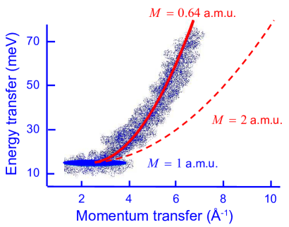
Figure 4: Schematic representation of incoherent inelastic neutron scattering results from H₂ in carbon nanotubes, with incident neutron energy $E_{0}=90$ meV [56, Fig. 1]. The translation motion of the recoiling H₂ molecules causes the observed continuum of intensity, usually called roto-recoil (white-blue ribbon), starting at the well visible first rotational excitation of H₂ being centered at $E\approx 14.7$ meV and $K\approx 2.7$ Å^-1 (blue ellipsoid). The $K-E$ position of the latter is in agreement with conventional theory. In contrast, a detailed fit (red parabola; full line) to the roto-recoil data reveals a strong reduction of the effective mass of recoiling H₂, which appears to be only 0.64 a.m.u. The red broken line (on the right) represents the conventional-theoretical parabola with effective mass 2 a.m.u. For details of data analysis see [56].

Moreover, the authors provide a detailed analysis of the roto-recoil data from incoherent inelastic neutron scattering, as shown in Fig. 4, and extracted a strongly reduced effective mass of the whole recoiling H₂ molecule (left parabola, red full line); see Eq. (13):

$$\textrm{recoil:}\ \ \ \ {M}_{\textrm{eff}}(\textrm{H}_{2})\approx 0.64\pm 0.07\ \ \textrm{a.m.u.}$$ (66)

This is in blatant contrast to the conventionally expected value $M(\textrm{H}_{2})=2.01$ a.m.u. for a freely recoiling H₂ molecule (right parabola, broken line). (Recall that the neutron-molecule collision does not break the molecular H-H bond.)

An extensive numerical analysis of the data is presented in [56], being based on time-of-flight data analysis (cf. Section 4) and the analysis of the measured data within conventional theory [40, 57].

This strong reduction of effective mass, which is far beyond any conceivable experimental error, corresponds to a strong reduction of momentum transfer by the factor $\leavevmode\nobreak\ 0.566$. Namely, the observed momentum transfer deficit is about $-43\%$ of the conventionally expected momentum transfer. This provides first experimental evidence of the new anomalous effect of momentum-transfer deficit in an elementary neutron collision with a recoiling molecule.

Recall that, as explained above (see subsection 4.2), every H₂-substrate binding must increase the molecule’s effective mass. Thus these findings from incoherent inelastic neutron scattering are in clear contrast to every conventional (classical or quantum) theoretical expectation. However, they have a natural (albeit qualitative, at present) interpretation in the frame of modern theory of weak values and two-state-vector formalism.

Incidentally, it may be noted that in principle the same calibration of ARCS was used in both experiments [47] and [56].

6.2.1 Comparison with a related 1-dimensional experiment

The above experimental results also show that the two-dimensional spectroscopic technique, as offered by the advanced time-of-flight spectrometer ARCS, represents a powerful method that provides novel insights into quantum dynamics of molecules and condensed matter. Clearly, this is due to the fact that $K$ and $E$ transfers can be measured over a broad region of the $K$–$E$ plane. This advantage makes these new instruments superior to the common one-dimensional ones (like TOSCA at ISIS spallation source, UK), in which the detectors can only measure along a specific trajectory in the $K$–$E$ plane. (TOSCA measures along two such trajectories [59].)

As an example, consider the results of [58] from molecular H₂ adsorbed in single-wall carbon nanotubes (which is similar to the material of [56]) at $T\approx 20$ K, investigated with TOSCA. Also this paper reports the measurement of the roto-recoil spectrum, but as a function of $E$ only. Therefore the strong anomalous effect (66) remained unnoticed, and for the theoretical analysis of the data the mass of H₂ was fixed to its conventionally expected value of 2 a.m.u.; see [58, p. 903].

6.2.2 Theoretical remarks

The large value of observed momentum transfer deficit in this experiment indicates that the theoretical condition of weakness is not fulfilled in this case. Therefore, here we should mention the theoretical results by Oreshkov and Brun [60] which show that weak measurements are universal, in the sense that every generalized measurement can be decomposed into a sequence of weak measurements; see remarks in subsection 7.2(J). This implies that the striking experimental result under consideration may still belong to the range of applicability of the new theory of weak values and two-state-vector formalism.

In this context, a speculative semi-quantitative treatment of the effect’s magnitude can be as follows. A formal limit $\lambda\rightarrow 1$—which however is theoretically treated in various works, e.g. [37]; cf. subsection 7.2(J)—taken in the above results shows that the special case $(C)$ predicts a $-50\%$ momentum transfer deficit (measured by the neutron), thus being comparable with the experimental value of $-43\%$; see above. Additionally, the applied low excitation energy of 90 meV further supports the physical assumption that the excitation is sufficiently soft in order that the envelope of the ground state $\Xi(P)_{i}$ is only slightly deformed, and thus the special case $(C)$ applies.

It may be noted that this assumption about the final atomic state is very common in the context of femtosecond dynamics in pump-probe optical experiments on molecules: A pump pulse lifts the (Gaussian) ground-state to an excited non-stationary state impulsively, keeping its initial shape (or envelope) unchanged.

6.3 Consequences for instrumental calibration

The theoretical analysis and results presented above have considerable implications for the calibration of the associated time-of-flight spectrometers. In particular, in neutron Compton scattering experiments it is a common practice to use the recoil peaks of certain light atoms (typically He or H) to achieve a refined calibration of the spectrometer. That is, the measured $(K,E)$-positions of a peak—together with the standard free-atom recoil expression of Eq. (13), sometimes also including conventional final-state effects—are used in order to fine tune the numerical values of (some of) the instrument parameters $(L_{0},L_{1}^{\theta},t_{0},\theta,E_{0})$ determining the measured time-of-flight values, Eq. (7). Obviously, such a calibration leads automatically to an (artificial) agreement of the data with conventional theory, thus being illegitimate for testing the new predictions of weak measurement and two-state-vector formalism against those of conventional theory.

7 Discussion

7.1 Reconsidering what is actually measured

In view to the above surprising experimental findings, it may be helpful to reconsider them with the aim to point out what is actually measured in the experiment, and what is usually assumed (implicitly or explicitly).

First of all, it should be reminded that all experimental results shown in the figures of Section 6 are in fact neutron data, which are converted to H data with the aid of the conventionally assumed theoretical relations

$$E_{H}=E_{n}\ \ \ \ \textrm{and}\ \ \ \ \hbar K_{H}=-\hbar K_{n}.$$ (67)

These relations are often considered as trivial or self-evident, being (tacitly) based on the assumption that the considered process is a two-body impulsive and incoherent (see Section 4) collision, with an additional assumption concerning the (effective) mass of the scattering particle.

The experimental data $(K_{n},E_{n})$ measured with the flight-of-time spectrometer is to be compared with the differing (!) predictions of the two alternative theories under consideration.

In the framework of the new theory (i.e. weak measurement and two-state-vector formalism), it is important to realize that, in general, the impulsive collision creates an entangled [61] (or a least discordant [62]) neutron-H quantum state; see also subsection 7.2(F). Very shortly after the considered collision, the H-atom becomes observed, or measured, by its close environment (i.e. adjacent atoms), which of course changes the quantum-correlation content [62] of the neutron-H state. Later on, the (spatial position of the) scattered neutron becomes strongly measured by the neutron detector—which concludes the experiment. In the context of the theoretical model of Section 5, taking into account the the environment of the scattering H-atom, we have:

$$E_{\textrm{H+env}}=E_{n}\ \ \ \ \textrm{and}\ \ \ \ \hbar K_{\textrm{H+env}}=-\hbar K_{n}$$ (68)

assuming again energy and momentum conservation for the case that the environment of the scattering H is not neglected. Then, $E_{n}=E_{\textrm{H+env}}$ corresponds to a momentum $\hbar K_{A}$ transferred on the scattering system ($A$ being here the system H+environment). The theoretically derived momentum transfer deficit, when interpreted in terms of conventional theory, is equivalent to a reduced effective mass of the whole H+environment system; i.e. the mass of the latter appears to be smaller than the mass of a free H-atom.

This weakness of conventional theory is further demonstrated by the results of the experiment by Olsen et al. [56], as presented in subsection 6.2; see also subsection 7.2(E). In contrast, the contradictions and/or inconsistencies of conventional theory just disappear in the framework of weak measurement and two-state-vector formalism, and at the same time, the experimental findings at issue are consistent with the new theoretical prediction of quantum momentum transfer deficit; see Section 5. In particular, the experimental results appear to be due to a characteristic feature of weak measurement and two-state-vector formalism being unknown in conventional theory, i.e. the specific quantum interference associated with the finite width of the final (i.e. post-selected) atomic state in momentum space and the basic formula of the weak value of atomic momentum.

7.2 Further remarks

(A) Until now, weak values are measured with a different degree of freedom of the same quantum system. Remarkably, in our approach, the two operators $\hat{q}$ and $\hat{P}$ occurring in the von Neumann interaction Hamiltonian of Eq. (45) refer to two different quantum systems. Thus, according to Vaidman [12], the concept of weak value arises here due to the interference of a quantum entangled wave and therefore it has no analog in classical wave interference. This further supports the conclusion that weak value is a genuinely quantum concept.

(B) To some people, post-selection roughly means “throwing some data out”. In the experimental context at issue, however, it rather means “performing a concrete measurement on the system at all, and analyzing the measured data only”.

Since the concepts of post-selection and associated quantum interference play a central role in this study, let us stress the following point. Strict energy conservation in the neutron-atom collision (see Section 4, Eq. (12)) reads

$$E\equiv E_{0}-E_{1}=\frac{(\hbar\mathbf{K}+\mathbf{P})^{2}}{2M}-\frac{P^{2}}{2M}.$$ (69)

Let us consider the idealized case in which the numerical values of both neutron energies $E_{i}$ ($i=0,1$) are sharply known—as conventional theory does by assuming plane waves for the neutron’s initial and final states. (As explained in Section 4, the detector measures a time-of-flight value, from which $E_{1}$ is derived if $E_{0}$ is pre-selected.) Then, as the initial atomic momentum ${\mathbf{P}}$ can take a range of values around ${\mathbf{P}}=0$ (due to the width of the atomic initial state $\Xi({\mathbf{P}})_{i}$), the momentum transfer satisfying this equation can take various values too. In other words, there are many Feynman paths starting at $|E_{0}\rangle$ and ending at the $|E_{1}\rangle$, the latter being located at the neutron detector. (These paths are interconnected with associated atomic paths.) Thus these paths must be coherently superposed before the scattering probability of the neutron is calculated. But as pointed out above (in subsection 4.1), the formalism of conventional neutron scattering theory fails to achieve this; e.g. its basic result (25) for the impulse approximation contains only the diagonal part, Eq. (26), of the initial-state atomic density operator $(|\Xi\rangle\langle\Xi|)_{i}$, and no explicit detail of the atomic final state. In contrast, the theoretical approach of weak values and two-state-vector formalism (Section 5) succeeds to achieve this goal.

In the frame of two-state-vector formalism, however, and also making contact with Danan’s et al. paper [36], the physical picture is substantially different from the conventional one. The formulas of two-state-vector formalism imply that the scattering under consideration is determined by the overlapping region—of momentum space, in our case—of both the forward- and backward-evolving quantum waves of the whole neutron+atom system. Concerning the atomic states, this overlap is obvious in the expressions of $P_{w}$. Additionally, looking at Eq. (69) we see that also the backward-evolving neutron state $\langle E_{1}|$ is consistent with a variety of atomic momenta ${\mathbf{P}}$ and accompanying momentum transfers $\hbar{\mathbf{K}}$. Clearly, all associated Feynman paths connecting $|E_{0}\rangle$ with $|E_{1}\rangle$ contribute to the considered neutron-atom collision.

(C) The derived quantum deficit of momentum transfer, $-\pi(\hbar K_{A})$, bears some resemblance to the theoretical result by Aharonov et al. discussed in Section 3, in which an interferometer mirror was pulled inwards due to proper post-selection, despite the photon momentum pushing it in the opposite direction [38]. The innovation of the derived result in Eq. (60) in comparison to the theoretical results of Ref. [38] is the direct applicability of (60) to a widely known subfield of experimental neutron physics (and possibly also to further fields of scattering physics), as shown in Section 6.

(D) In the physical context of the incoherent neutron scattering experiment of subsection 6.1, the following remarks cannot be overemphasized: Conventionally expected deviations from the impulse approximation, Eq. (13), (widely known as final-state effects [42]) must give peak shifts to less than $\hbar\omega_{\textrm{rec}}$, since they are always caused by the atom not being free, owing to its interaction with other atoms. Thus there is an additional resistance to motion of the struck atom, which effectively increases its mass and thus causes a slightly lower energy transfer than the conventionally expected $\hbar\omega_{\textrm{rec}}$. Summarizing, a peak-maximum shift to higher energies than $\hbar\omega_{\textrm{rec}}$ seems impossible within conventional theory; see subsection 4.2 and [42, 44, 49].) Hence the considered experimental results, and the additional ones reported in [54] showing the same peak-shifts to higher energy transfers, contradict conventional theoretical expectations even qualitatively.

(E) Moreover, the results of [56] discussed in subsection 6.2 appear contradictory—in the light of conventional theory—because of the following two main points:

$(1)$ The observed $J=0\rightarrow 1$ rotational excitation of the H₂ molecule by incoherent scattering exhibits an effective mass of $\ \approx 1$ a.m.u., Eq. (65), as conventionally expected, since the neutron may be expected to exchange energy and momentum with a single H.

$(2)$ However, in the same experiment, the effective mass of the observed roto-recoil response of the whole H₂ molecule is not 2 a.m.u. (because the whole molecule undergoes a translational motion), but only $\approx 0.64$ a.m.u., Eq. (66)—which is clearly meaningless in the frame of conventional theory.

As explained above, in conventional theory, depending on the specific constrains of measurement, a decrease of effective mass is equivalent to $(a)$ an anomalous increased energy transfer, or equivalently $(b)$ a decreased momentum transfer. In both its forms $(a)$ and $(b)$, the observed effect appears—if interpreted within the framework of conventional scattering theory—to contradict the basic laws of energy and/or impulse conservation. In contrast, in the theoretical frame of weak measurement, this contradiction dissolves.

In this context, note also that exotic mass and momentum values of weak measurements have been already mentioned in [11, Section G.3].

(F) As emphasized above, neutron-atom (or neutron-nucleus) entanglement [61] or quantum discord [62], caused by their scattering interaction, play absolutely no role in conventional theory of neutron scattering [40, 41, 42].

Moreover, in neutron Compton scattering a second approximation is introduced by hand: The complete $N$-body Hamiltonian of the scattering system is replaced with an effective Hamiltonian of one particle being captured in some effective Born–Oppenheimer potential [42, 43]. Obviously this assumption is tantamount to considering all interparticle entanglement or quantum discord (and the associated decoherence appearing within the collisional time-window [63]) as being irrelevant.

(G) Considerable efforts have been made during the last 25 years to compare Born–Oppenheimer potentials calculated with quantum-chemistry methods with associated quantities derived from several neutron Compton scattering data sets; cf. [42] and references therein. In the light of the present investigation, however, these comparisons appear to have a rather approximative character, thus being less quantitative than claimed in the related publications.

To be more specific, let us mention the following details. The overwhelming part of neutron Compton scattering (or deep inelastic neuron scattering) investigations are dealing with measurements of Compton profiles (i.e. the distribution of initial atomic momenta along a given spatial direction), from which one may derive (properties of) the associated single-particle Born–Oppenheimer potential. The preceding theoretical results, however, strongly question the validity of the standard method of data analysis for the following reason.

As shown in Section 5, the weak measurement-theoretical deficit $-\pi(\hbar K_{A})$ should depend on the considered momentum transfer $\hbar K_{A}$. This should cause an anomalous distortion of the conventionally expected Compton profile, which conventional theory assumes to be an even function for isotropic systems. Namely, each point of the lower-momentum Compton peak-wing should receive a larger weak value-shift $\pi(\hbar K)$ than a corresponding point of the higher-momentum wing. Consequently, the widely applied symmetrization procedure of the measured Compton profile (to remove partially deviations from the impulse approximation; see [42]) should introduce artificial features to the derived Compton profile and derived Born–Oppenheimer potential. Especially for scattering from H the Compton peak-width is particularly large (with respect to the instrumental resolution) and thus the considered distortion should be measurable. (This remark does not apply to the data of Fig. 3; see subsection 6.1.)

(H) The derivations of Section 5 apply to an impulsive two-particle collision, e.g. of a neutron with an initially localized atom at rest. Since the scattering at issue is incoherent—i.e. in each collision a neutron exchanges energy and momentum with one scattering particle only—they apply directly to condensed and/or interacting systems (like those considered in Section 6), where the scattering atoms are parts of a molecule, or are adsorbed on surfaces or nanocavities, etc. Thus a scattering atom interacts with adjacent particles of its environment which is tantamount to a spatial confinement. The latter causes a finite width of the initial atomic state $\Xi_{i}$, and to less extend of its final state $\Xi_{f}$—both appearing to play an equally important role in the quantum interference captured in the weak value-calculations of subsection 5.2.

Based on these physical considerations, we may conclude that the dynamics of the scattering atom should also depend on the dynamics of the environment (which in general is also a quantum system), and that the collisional process is therefore not a strict two-body dynamical problem, as standardly assumed in the impulse approximation of conventional theory; see [42, 43]. Especially, it is satisfying that the theoretical frame of weak values and two-state-vector formalism takes care of these finite widths of the initial and final atomic states (see subsection 5.2.2), and in particular reveals the significance of the final-state width which plays a minor role in conventional theory of impulse approximation [42] and its extensions.

(I) The remarks of points (G) and (H) support the opinion that weak values are novel quantum interference phenomena in which post-selection plays a crucial role [12, 32, 33, 35, 37]. This opinion gets additional support by the quantum Cheshire cat effect [64, 65], which however has found a classical analogue in a recent experiment with continuous light beams [66]. In this regard, see also the work by Di Lorenzo [67] who shows that the quantum Cheshire cat is a consequence of quantum interference, that it is present also for intermediate-strength measurements, and that it is a rather common occurrence in post-selected measurements.

Further support of the quantum character of the Cheshire cat effect is presented by the generalization to the case that the pre- and the post-selections are entangled with each other [68], in which case there is no classical analogue to this new Cheshire cat scheme.

(J) Generalizing the weak measurement formalism, Oreshkov and Brun have shown [60] that weak measurements are universal, in the sense that any generalized measurement can be decomposed into a sequence of weak measurements. This important theoretical result is further supported by the work of Qin et al. [37], who showed that the main weak measurement results can be extended to the realm of arbitrary measurement strength.

This finding may have important applications to further collisional experiments than the incoherent neutron scattering at issue. For example, energy and momentum transfers of various particles are the primarily measured quantities in relativistic (high-energy) collision experiments too. Due to their complexity, full details of the measurement methods and detection systems are usually not described in the related publications. However it seems natural to believe that the above theoretical investigations can be extended to the relativistic scattering regime. Thus one may wonder whether the anomalous decrease of effective mass derived above can affect related relativistic measurements.

For example, the mass of the celebrated Higgs boson was measured in proton-proton collisions and recently reported to be ca. 125 GeV [69]. At the same time, various categories of data (corresponding to various decay channels) can be post-selected in order to determine the Higgs boson mass, and thus it would be interesting to examine whether there might exist significant differences between the values of the mass correspondingly determined; cf. Fig. 1 of [69] in which such a (small) difference is visible.

(K) As mentioned above, a discussion concerning interpretation and/or physical meaning of the concepts of weak value and two-state-vector formalism is beyond the scope of this paper. However, it may be helpful for non-specialized or skeptical readers to consider Mermin’s related descriptions of some examples and results of weak values and two-state-vector formalism [70] using a more common scientific language.

Concluding, we feel that the theoretical formalism of weak values, weak measurement and two-state-vector formalism (which is really quantum) not only sheds new light on interpretational issues concerning fundamental quantum theory but it also offers a new guide for our intuition to predict, plan, and also carry out new experiments and reveal novel quantum effects.

References

- [1] Feynman RP, Leighton RB, Sands M. The Feynman Lectures on Physics, Vol. III, Quantum Mechanics. Pasadena, California: California Institute of Technology, 2013. http://www.feynmanlectures.caltech.edu/
- [2] Wheeler JA, Zurek WH. Quantum Theory and Measurement. Princeton: Princeton University Press, 1983.
- [3] Wiseman HM, Milburn GJ. Quantum Measurement and Control. Cambridge: Cambridge University Press, 2009.
- [4] Nielsen MA, Chuang IL. Quantum Computation and Quantum Information. Cambridge: Cambridge University Press, 2000.
- [5] Schlosshauer M. Decoherence and the Quantum-To-Classical Transition. The Frontiers Collection, Berlin: Springer, 2007. doi:10.1007/978-3-540-35775-9
- [6] Aharonov Y, Rohrlich D. Quantum Paradoxes: Quantum Theory for the Perplexed. Weinheim: Wiley-VCH, 2005.
- [7] Kofman AG, Ashhab S, Nori F. Nonperturbative theory of weak pre- and post-selected measurements. Physics Reports 2012; 520(2): 43–133. arXiv:1109.6315, doi:10.1016/j.physrep.2012.07.001
- [8] Tamir B, Cohen E. Introduction to weak measurements and weak values. Quanta 2013; 2(1): 7–17. doi:10.12743/quanta.v2i1.14
- [9] Svensson BEY. Pedagogical review of quantum measurement theory with an emphasis on weak measurements. Quanta 2013; 2(1): 18–49. doi:10.12743/quanta.v2i1.12
- [10] Dressel J, Malik M, Miatto FM, Jordan AN, Boyd RW. Understanding quantum weak values: Basics and applications. Reviews of Modern Physics 2014; 86(1): 307–316. arXiv:1305.7154, doi:10.1103/RevModPhys.86.307
- [11] Aharonov Y, Cohen E, Elitzur AC. Foundations and applications of weak quantum measurements. Physical Review A 2014; 89(5): 052105. doi:10.1103/PhysRevA.89.052105
- [12] Vaidman L. Comment on “How the result of a single coin toss can turn out to be 100 heads”. 2014; arXiv:1409.5386
- [13] Aharonov Y, Vaidman L. Properties of a quantum system during the time interval between two measurements. Physical Review A 1990; 41(1): 11–20. doi:10.1103/PhysRevA.41.11
- [14] Aharonov Y, Popescu S, Tollaksen J. A time-symmetric formulation of quantum mechanics. Physics Today 2010; 63(11): 27–32. doi:10.1063/1.3518209
- [15] Aharonov Y, Albert DZ, Vaidman L. How the result of a measurement of a component of the spin of a spin- particle can turn out to be 100. Physical Review Letters 1988; 60(14): 1351–1354. doi:10.1103/PhysRevLett.60.1351
- [16] Aharonov Y, Bergmann PG, Lebowitz JL. Time symmetry in the quantum process of measurement. Physical Review B 1964; 134(6): 1410–1416. doi:10.1103/PhysRev.134.B1410
- [17] Duck IM, Stevenson PM, Sudarshan ECG. The sense in which a “weak measurement” of a spin- particle’s spin component yields a value 100. Physical Review D 1989; 40(6): 2112–2117. doi:10.1103/PhysRevD.40.2112
- [18] von Neumann J. Mathematische Grundlagen der Quantenmechanik. Berlin: Springer Verlag, 1932. [Mathematical Foundations of Quantum Mechanics. Princeton: Princeton University Press, 1955.]
- [19] Hosten O, Kwiat P. Observation of the spin Hall effect of light via weak measurements. Science 2008; 319(5864): 787–790. doi:10.1126/science.1152697
- [20] Dixon PB, Starling DJ, Jordan AN, Howell JC. Ultrasensitive beam deflection measurement via interferometric weak value amplification. Physical Review Letters 2009; 102(17): 173601. arXiv:0906.4828, doi:10.1103/PhysRevLett.102.173601
- [21] Lundeen JS, Sutherland B, Patel A, Stewart C, Bamber C. Direct measurement of the quantum wavefunction. Nature 2011; 474(7350): 188–191. arXiv:1112.3575, doi:10.1038/nature10120
- [22] Kocsis S, Braverman B, Ravets S, Stevens MJ, Mirin RP, Shalm LK, Steinberg AM. Observing the average trajectories of single photons in a two-slit interferometer. Science 2011; 332(6034): 1170–1173. doi:10.1126/science.1202218
- [23] Wiseman HM. Weak values, quantum trajectories, and the cavity-QED experiment on wave-particle correlation. Physical Review A 2002; 65(3): 032111. arXiv:quant-ph/0112116, doi:10.1103/PhysRevA.65.032111
- [24] Di Lorenzo A, Egues JC. Weak measurement: Effect of the detector dynamics. Physical Review A 2008; 77(4): 042108. arXiv:0801.1814, doi:10.1103/PhysRevA.77.042108
- [25] Zhu X, Zhang Y, Pang S, Qiao C, Liu Q, Wu S. Quantum measurements with preselection and postselection. Physical Review A 2011; 84(5): 052111. arXiv:1108.1608, doi:10.1103/PhysRevA.84.052111
- [26] Pang S, Wu S, Chen Z-B. Weak measurement with orthogonal preselection and postselection. Physical Review A 2012; 86(2): 022112. doi:10.1103/PhysRevA.86.022112
- [27] Gisin N. Quantum measurement of spins and magnets, and the classical limit of PR-boxes. 2014; arXiv:1407.8122
- [28] Silva R, Gisin N, Guryanova Y, Popescu S. Multiple observers can share the nonlocality of half of an entangled pair by using optimal weak measurements. Physical Review Letters 2015; 114(25): 250401. arXiv:1408.2272, doi:10.1103/PhysRevLett.114.250401
- [29] Jordan AN, Martinez-Rincon J, Howell JC. Technical advantages for weak-value amplification: When less is more. Physical Review X 2014; 4(1): 011031. doi:10.1103/PhysRevX.4.011031
- [30] Zhang L, Datta A, Walmsley IA. Precision metrology using weak measurements. Physical Review Letters 2015; 114(21): 210801. arXiv:1310.5302, doi:10.1103/PhysRevLett.114.210801
- [31] Ferrie C, Combes J. How the result of a single coin toss can turn out to be 100 heads. Physical Review Letters 2014; 113(12): 120404. arXiv:1403.2362, doi:10.1103/PhysRevLett.113.120404
- [32] Romito A, Jordan AN, Aharonov Y, Gefen Y. Weak values are quantum: you can bet on it. Quantum Studies: Mathematics and Foundations 2016; 3(1): 1–4. arXiv:1508.06304, doi:10.1007/s40509-015-0069-z
- [33] Parks AD, Gray JE. A note concerning von Neumann projector measurement pointer states, weak values, and interference. 2012; arXiv:1208.1029
- [34] Pati AK, Wu J. Conditions for anomalous weak value. 2014; arXiv:1410.5221
- [35] Dressel J. Weak values as interference phenomena. Physical Review A 2015; 91(3): 032116. arXiv:1410.0943, doi:10.1103/PhysRevA.91.032116
- [36] Danan A, Farfurnik D, Bar-Ad S, Vaidman L. Asking photons where have they been. Physical Review Letters 2013; 111(24): 240402. arXiv:1304.7469, doi:10.1103/PhysRevLett.111.240402
- [37] Qin L, Feng W, Li X-Q. Simple understanding of quantum weak values. Scientific Reports 2016; 6: 20286. arXiv:1505.00595, doi:10.1038/srep20286
- [38] Aharonov Y, Botero A, Nussinov S, Popescu S, Tollaksen J, Vaidman L. The classical limit of quantum optics: not what it seems at first sight. New Journal of Physics 2013; 15(9): 093006. arXiv:1305.0168, doi:10.1088/1367-2630/15/9/093006
- [39] Scully MO, Zubairy MS. Quantum Optics. Cambridge: Cambridge University Press, 1997.
- [40] Squires GL. Introduction to the Theory of Thermal Neutron Scattering. Mineola: Dover Publications, 1996.
- [41] Lovesey SW. Theory of Neutron Scattering from Condensed Matter. Oxford: Oxford University Press, 1984.
- [42] Watson GI. Neutron Compton scattering. Journal of Physics: Condensed Matter 1996; 8(33): 5955–5975. doi:10.1088/0953-8984/8/33/005
- [43] Tietje IC. Neutron Compton scattering – critical analysis of some basic theoretical assumptions. Journal of Physics: Conference Series 2012; 380(1): 012014. doi:10.1088/1742-6596/380/1/012014
- [44] Sears VF. Scaling and final-state interactions in deep-inelastic neutron scattering. Physical Review B 1984; 30(1): 44–51. doi:10.1103/PhysRevB.30.44
- [45] Bonham RA, Cooper G, Hitchcock AP. Electron Compton-like quasielastic scattering from H2, D2, and HD. Journal of Chemical Physics 2009; 130(14): 144303. doi:10.1063/1.3108490
- [46] Bonham RA. A review of electron scattering cross section measurements by use of pulsed electron beam time of flight techniques. Journal of Electron Spectroscopy and Related Phenomena 2007; 155(1–3): 1–6. doi:10.1016/j.elspec.2006.11.003
- [47] Diallo SO, Azuah RT, Abernathy DL, Rota R, Boronat J, Glyde HR. Bose–Einstein condensation in liquid 4He near the liquid-solid transition line. Physical Review B 2012; 85(14): 140505. arXiv:1111.2284, doi:10.1103/PhysRevB.85.140505
- [48] Oak Ridge National Laboratory. Wide Angular-Range Chopper Spectrometer. http://neutrons.ornl.gov/ARCS
- [49] Stringari S. Scaling and deep inelastic neutron scattering from quantum liquids and solids. Physical Review B 1987; 35(4): 2038–2040. doi:10.1103/PhysRevB.35.2038
- [50] Taylor JR. Scattering Theory: The Quantum Theory of Nonrelativistic Collisions. New York: Wiley, 1972.
- [51] van Hove L. Correlations in space and time and Born approximation scattering in systems of interacting particles. Physical Review 1954; 95(1): 249–262. doi:10.1103/PhysRev.95.249
- [52] Popescu S. Dynamical quantum non-locality. Nature Physics 2010; 6(3): 151–153. doi:10.1038/nphys1619
- [53] Aharonov Y, Cohen E, Ben-Moshe S. Unusual interactions of pre-and-post-selected particles. EPJ Web of Conferences 2014; 70: 00053. arXiv:1208.3203, doi:10.1051/epjconf/20147000053
- [54] Stock C, Cowley RA, Taylor JW, Bennington SM. High-energy neutron scattering from hydrogen using a direct geometry spectrometer. Physical Review B 2010; 81(2): 024303. arXiv:0907.1945, doi:10.1103/PhysRevB.81.024303
- [55] Science and Technology Facilities Council. MARI. http://www.isis.stfc.ac.uk/instruments/MARI/
- [56] Olsen RJ, Beckner M, Stone MB, Pfeifer P, Wexler C, Taub H. Quantum excitation spectrum of hydrogen adsorbed in nanoporous carbons observed by inelastic neutron scattering. Carbon 2013; 58: 46–58. doi:10.1016/j.carbon.2013.02.026
- [57] Mitchell PCH, Parker SF, Ramirez-Cuesta AJ, Tomkinson J. Vibrational Spectroscopy with Neutrons. World Scientific: New Jersey, 2005.
- [58] Georgiev PA, Ross DK, De Monte A, Montaretto-Marullo U, Edwards RAH, Ramirez-Cuesta AJ, Adams MA, Colognesi D. In situ inelastic neutron scattering studies of the rotational and translational dynamics of molecular hydrogen adsorbed in single-wall carbon nanotubes (SWNTs). Carbon 2005; 43(5): 895–906. doi:10.1016/j.carbon.2004.11.006
- [59] Science and Technology Facilities Council. TOSCA. http://www.isis.stfc.ac.uk/instruments/TOSCA/
- [60] Oreshkov O, Brun TA. Weak measurements are universal. Physical Review Letters 2005; 95(11): 110409. arXiv:quant-ph/0503017, doi:10.1103/PhysRevLett.95.110409
- [61] Horodecki R, Horodecki P, Horodecki M, Horodecki K. Quantum entanglement. Reviews of Modern Physics 2009; 81(2): 865–942. arXiv:quant-ph/0702225, doi:10.1103/RevModPhys.81.865
- [62] Modi K, Brodutch A, Cable H, Paterek T, Vedral V. The classical-quantum boundary for correlations: Discord and related measures. Reviews of Modern Physics 2012; 84(4): 1655–1707. arXiv:1112.6238, doi:10.1103/RevModPhys.84.1655
- [63] Chatzidimitriou-Dreismann CA, Stenholm S. On correlation approach to scattering in the decoherence timescale. Towards the theoretical interpretation of neutron and electron Compton scattering experimental findings. In: Decoherence, Entanglement and Information Protection in Complex Quantum Systems. Akulin VM, Sarfati A, Kurizki G, Pellegrin S (editors), NATO Science Series II: Mathematics, Physics and Chemistry, vol.189, Dordrecht: Springer, 2005, pp. 555–562. arXiv:quant-ph/0702038, doi:10.1007/1-4020-3283-8_37
- [64] Aharonov Y, Popescu S, Skrzypczyk P. Quantum Cheshire cats. New Journal of Physics 2013; 15(11): 113015. arXiv:1202.0631, doi:10.1088/1367-2630/15/11/113015
- [65] Denkmayr T, Geppert H, Sponar S, Lemmel H, Matzkin A, Tollaksen J, Hasegawa Y. Observation of a quantum Cheshire Cat in a matter-wave interferometer experiment. Nature Communications 2014; 5: 4492. doi:10.1038/ncomms5492
- [66] Atherton DP, Ranjit G, Geraci AA, Weinstein JD. Observation of a classical Cheshire cat in an optical interferometer. Optics Letters 2015; 40(6): 879–881. arXiv:1410.2267, doi:10.1364/OL.40.000879
- [67] Di Lorenzo A. Hunting for the quantum Cheshire cat. 2012; arXiv:1205.3755
- [68] Guryanova Y, Brunner N, Popescu S. The complete quantum Cheshire cat. 2012; arXiv:1203.4215
- [69] G. Aad et al. (ATLAS Collaboration, CMS Collaboration). Combined measurement of the Higgs boson mass in collisions at and 8 TeV with the ATLAS and CMS experiments. Physical Review Letters 2015; 114(19): 191803. doi:10.1103/PhysRevLett.114.191803
- [70] Mermin ND. Consistent treatments of quantum mechanics. Physics Today 2011; 64(10): 8–9. doi:10.1063/PT.3.1271