High harmonic generation in Landau-quantized graphene subjected to a strong electromagnetic radiation

Abstract

We study nonlinear optical response of Landau quantized graphene to an intense electromagnetic wave. In particular, we consider high harmonic generation process. It is shown that one can achieve efficient generation of high harmonics with strong radiation fields – when the work of the wave electric field on the magnetic length is larger than pump photon energy. At that high harmonics generation process takes place for a wide range of the pump wave frequencies and intensities even for significant broadening of Landau levels because of impurities in graphene.

I INTRODUCTION

Thanks to exotic nonlinear electromagnetic properties of graphene Nov1 , the latter is extensively considered as an active material for diverse optical applications Nov2 . Note that the graphene is an effective material for multiphoton interband excitation, wave mixing, and harmonic generation processes 25 ; 26 ; 27 ; 28 ; 30 ; Mer1 ; Mer2 ; Mer3 ; Mer4 . When a static uniform magnetic field is applied perpendicular to the graphene plane, the electron energy is quantized forming nonequidistant Landau levels (LLs). As a consequence, in the graphene the anomalous quantum Hall effect takes place Nov3 ; Zhang ; GS ; Goer .

While most of the works have concentrated on static or linear optical properties of the Landau-quantized graphene, one direction that has not been fully explored is the nonlinear response of Landau-quantized graphene to a strong coherent radiation. Linear optical response of graphene quantum Hall system with the different aspects have been studied in Refs. MHA ; AC1 ; AC2 ; AC3 ; AC4 ; LLL1 ; Ferreira . Ultrafast carrier dynamics and carrier multiplication in Landau-quantized graphene have been investigated in Refs. Carrier1 ; Carrier2 . In Refs. LLL1 ; LLL2 tunable graphene-based laser on the Landau levels in the terahertz regime have been proposed. Interesting effects also arise in the high frequency regime. As was shown in Ref. MHA the plateau structure in the quantum Hall effect in graphene is retained, up to significant degree of disorder, even in the ac (THz) regime, although the heights of the plateaus are no longer quantized. In Refs. Mer5 ; Mer6 the nonlinear optical response of graphene and semiconductor-hetero-structures to a moderately strong laser radiation in the quantum Hall regime, in particular, radiation intensity at the 3rd harmonic, as well as nonlinear Faraday effect have been investigated. It has been shown that 3rd harmonic radiation intensity has a characteristic Hall plateau structures that persist for a wide range of the pump wave frequencies and intensities even for significant broadening of Landau levels because of impurities in graphene. With further increase of pump wave intensity and due to the peaks in the density of states one can also expect enhancement of the high harmonics’ radiation power in Landau-quantized graphene. Hence, it is of interest to consider high harmonics generation process in the ultrastrong wave-graphene coupling regime. Moreover, the energy range of interest lies in the THz and Mid Infrared domain where high-power generators and frequency multipliers are of special interest.

In the present work, a microscopic theory of the Landau-quantized graphene interaction with strong coherent electromagnetic radiation is presented. Our calculations show that one can achieve efficient generation of high harmonics with strong radiation fields – when the work of the wave electric field on the magnetic length is Considerably larger than pump photon energy. At that for optimization we investigate high harmonics generation process depending on the pump wave frequency, intensity and broadening of LLs.

The paper is organized as follows. In Sec. II the Hamiltonian which governs the quantum dynamics of considered process and the set of equations for a single-particle density matrix are presented. In Sec. III, we numerically solve obtained equations and consider high harmonics generation process. Finally, conclusions are given in Sec. IV.

II BASIC MODEL

The sketch of the considered scheme for harmonics generation is shown in Fig. 1. The graphene sheet is taken in the $xy$ plane ($z=0$) and a uniform static magnetic field is applied in the perpendicular direction. A plane linearly polarized (along the $x$ axis) quasimonochromatic electromagnetic radiation of carrier frequency $\omega_{0}$ and slowly varying envelope $E_{0}(t)$ interacts with the such system. Under these circumstances the Hamiltonian of the system in the second quantization formalism in the presence of a uniform time-dependent electric field

$$E(t)=E_{0}(t)\cos\omega_{0}t$$ (1)

can be presented in the form Mer5 :

$$\widehat{H} = \sum\limits_{n=-\infty}^{\infty}\sum\limits_{m=0}^{N_{B}-1}\varepsilon_{n}\widehat{a}_{n,m}^{+}\widehat{a}_{n,m}$$ (2)

$$+\sum\limits_{n,n^{\prime}=-\infty}^{\infty}\sum\limits_{m=0}^{N_{B}-1}E(t)\mathcal{D}_{n,n^{\prime}}\widehat{a}_{n,m}^{+}\widehat{a}_{n^{\prime},m},$$

where $\widehat{a}_{n,m}^{\dagger}$ and $\widehat{a}_{n,m}$ are, respectively, the creation and annihilation operators for a carrier in a LL state. The energy spectrum is given by

$$\varepsilon_{n}=\mathrm{sgn}(n)\hbar\omega_{B}\sqrt{\left|n\right|},$$ (3)

where $\omega_{B}=\sqrt{2}\mathrm{v}_{F}/l_{B}$ plays the role of the cyclotron frequency, $\mathrm{v}_{F}$ is the Fermi velocity. Here $n$ is the LL index – for an electron $n>0$ and for a hole $n<0$. The extra LL with $n=0$ is shared by both electrons and holes. The LLs are degenerate upon second quantum number $m$ with the large degeneracy factor $N_{B}=\mathcal{S}/2\pi l_{B}^{2}$ which equals the number of flux quanta threading the 2D surface $\mathcal{S}$ occupied by the electrons. The magnetic length is $l_{B}=\sqrt{c\hbar/eB}$ ($e$ is the elementary charge, $\hbar$ is Planck’s constant, $c$ is the light speed in vacuum, and $B$ is the magnetic field strength). In Eq. (2) $\mathcal{D}_{n,n^{\prime}}$ is the dipole moment operator:

$$\mathcal{D}_{n,n^{\prime}}=\frac{iel_{B}}{2\sqrt{2}}\left[\varkappa_{n,n^{\prime}}\mathbb{\delta}_{\left|n\right|,\left|n^{\prime}\right|+1}+\varkappa_{n^{\prime},n}\mathbb{\delta}_{\left|n\right|,\left|n^{\prime}\right|-1}\right]\frac{\hbar\omega_{B}}{\varepsilon_{n^{\prime}}-\varepsilon_{n}},$$ (4)

where $\varkappa_{n,n^{\prime}}=\mathrm{sgn}(n)\sqrt{1+\delta_{n^{\prime},0}}$.

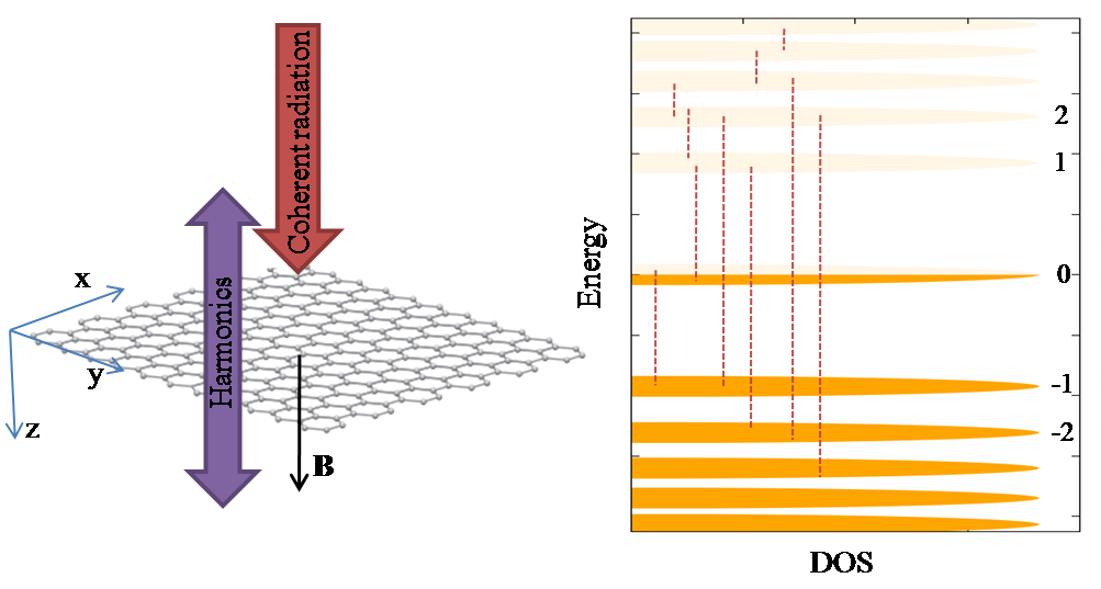
Figure 1: Schematic view of the considered scheme for generation of harmonics. The graphene sheet is taken in the xy plane (z=0) and a uniform static magnetic field is applied in the perpendicular direction. The optical excitation via a linearly polarized coherent radiation pulse induces the transitions between LLs which results surface currents and harmonics generation. On the right hand side we show a typical density of states for Landau-quantized graphene with some dipole allowed transitions.

Then we will pass to Heisenberg representation where operators obey the evolution equation

$$i\hbar\frac{\partial\widehat{L}}{\partial t}=\left[\widehat{L},\widehat{H}\right]$$

and expectation values are determined by the initial density matrix $\widehat{D}$: $<\widehat{L}>=Sp\left(\widehat{D}\widehat{L}\right)$. In order to develop microscopic theory of the nonlinear interaction of the graphene QHE system with a strong radiation field, we need to solve the Liouville-von Neumann equation for the single-particle density matrix

$$\rho(n_{1},m_{1};n_{2},m_{2},t)=<\widehat{a}_{n_{2},m_{2}}^{+}(t)\widehat{a}_{n_{1},m_{1}}(t)>.$$ (5)

For the initial state of the graphene quasiparticles we assume an ideal Fermi gas in equilibrium. According to the latter, the initial single-particle density matrix will be diagonal, and we will have the Fermi-Dirac distribution:

$$\rho(n_{1},m_{1};n_{2},m_{2},0)=\rho_{F}\left(n_{1}\right)\frac{\delta_{n_{1},n_{2}}\delta_{m_{1},m_{2}}}{1+\exp\left(\frac{\varepsilon_{n_{1}}-\varepsilon_{F}}{T}\right)},$$ (6)

$$\rho_{F}\left(n_{1}\right)=\frac{1}{1+\exp\left(\frac{\varepsilon_{n_{1}}-\varepsilon_{F}}{T}\right)}.$$ (7)

Including in Eq. (6) quantity $\varepsilon_{F}$ is the Fermi energy, $T$ is the temperature in energy units. As is seen from the interaction term in the Hamiltonian (2) quantum number $m$ is conserved: $\rho(n_{1},m_{1};n_{2},m_{2},t)=\rho_{n_{1},n_{2}}\left(t\right)\delta_{m_{1},m_{2}}$. To include the effect of the LLs broadening we will assume that it is caused by the disorder described by randomly placed scatterers. When the range of the random potential is larger than the lattice constant in graphene, the scattering between $K$ and $K^{\prime}$ points in the Brillouin zone is suppressed and we can assume homogeneous broadening of the LLs Ando . The latter can be incorporated into evolution equation for $\rho_{n_{1},n_{2}}\left(t\right)$ by the damping term $-i\Gamma_{n_{1},n_{2}}\rho_{n_{1},n_{2}}\left(t\right)$ and from Heisenberg equation one can obtain evolution equation for the reduced single-particle density matrix:

$$i\hbar\frac{\partial\rho_{n_{1},n_{2}}(t)}{\partial t}=\left[\varepsilon_{n_{1}}-\varepsilon_{n_{2}}-i\Gamma_{n_{1},n_{2}}\right]\rho_{n_{1},n_{2}}(t)$$

$$-E(t)\sum\limits_{n}\left[\mathcal{D}_{n,n_{2}}\rho_{n_{1},n}(t)-\mathcal{D}_{n_{1},n}\rho_{n,n_{2}}(t)\right].$$ (8)

For the norm-conserving damping matrix we take $\Gamma_{n_{1},n_{2}}=\Gamma\left(1-\delta_{n_{1},n_{2}}\right)$, where $\Gamma$ measures the Landau level broadening (see Fig. 1).

As is seen from Eqs. (8) and (4) in the Landau-quantized graphene, wave-particle interaction can be characterized by the dimensionless parameter $\chi_{0}=eE_{0}l_{B}/\hbar\omega_{0}$, which represents the work of the wave electric field $E_{0}$ on the magnetic length $l_{B}$ in units of photon energy $\hbar\omega_{0}$. Depending on the value of this parameter $\chi_{0}$, one can distinguish three different regimes in the wave-particle interaction process. Thus, $\chi_{0}<<1$ corresponds to the one-photon interaction regime, $\chi_{0}>>1$ corresponds to the static field limit, and $\chi_{0}\succsim 1$ to the multiphoton interaction regime. In this paper we consider just multiphoton interaction regime ($\chi_{0}>1$) and look for features in the harmonic spectra of the laser driven graphene.

III GENERATION OF HARMONICS AT THE MULTIPHOTON EXCITATION

The optical excitation via a linearly polarized coherent radiation pulse induces the transitions between LLs which results surface currents:

$$\mathcal{J}_{x}=-\frac{e\mathrm{v}_{F}}{\pi l_{B}^{2}}\sum\limits_{n,n^{\prime}}\rho_{n^{\prime},n}\left(\varkappa_{n,n^{\prime}}\mathbb{\delta}_{\left|n\right|,\left|n^{\prime}\right|+1}+\varkappa_{n^{\prime},n}\mathbb{\delta}_{\left|n\right|,\left|n^{\prime}\right|-1}\right),$$

$$\mathcal{J}_{y}=-\frac{ie\mathrm{v}_{F}}{\pi l_{B}^{2}}\sum\limits_{n,n^{\prime}}\rho_{n^{\prime},n}\left(\varkappa_{n^{\prime},n}\mathbb{\delta}_{\left|n\right|,\left|n^{\prime}\right|-1}-\varkappa_{n,n^{\prime}}\mathbb{\delta}_{\left|n\right|,\left|n^{\prime}\right|+1}\right).$$ (9)

Here we have taken into account the spin and valley degeneracy factors $g_{s}=2$ and $g_{v}=2$ and made summation over quantum number $m$ which yields the degeneracy factor $N_{B}$. These currents have nonlinear dependence on the pump wave field. At that one can expect intense radiation of harmonics of the incoming wave-field in the result of the coherent transitions between LLs. The harmonics will be described by the additional generated fields $E_{x,y}^{(g)}$. We assume that the generated fields are considerably smaller than the incoming field $\left|E_{x,y}^{(g)}\right|<<\left|E\right|$. In this case we do not need to solve self-consistent Maxwell’s wave equation with Eq. (8). To determine the electromagnetic field of harmonics we can solve Maxwell’s wave equation in the propagation direction with the given source term:

$$\frac{\partial^{2}E_{x,y}^{(t)}}{\partial z^{2}}-\frac{1}{c^{2}}\frac{\partial^{2}E_{x,y}^{(t)}}{\partial t^{2}}=\frac{4\pi}{c^{2}}\frac{\partial\mathcal{J}_{x,y}\left(t\right)}{\partial t}\delta\left(z\right).$$ (10)

Here $\delta\left(z\right)$ is the Dirac delta function, $E_{x,y}^{(t)}$ is the total field. The solution to equation (10) reads

$$E_{x,y}^{(t)}\left(t,z\right)=E_{x,y}\left(t-z/c\right)$$

$$-\frac{2\pi}{c}\left[\theta\left(z\right)\mathcal{J}_{x,y}\left(t-z/c\right)+\theta\left(-z\right)\mathcal{J}_{x,y}\left(t+z/c\right)\right],$$ (11)

where $\theta\left(z\right)$ is the Heaviside step function with $\theta\left(z\right)=1$ for $z\geq 0$ and zero elsewhere. The first term in Eq. (11) is the incoming wave. In the second line of Eq. (11), we see that after the encounter with the graphene sheet two propagating waves are generated. One traveling in the propagation direction of the incoming pulse and one traveling in the opposite direction. The Heaviside functions ensure that the generated light propagates from the source located at $z=0$. We assume that the spectrum is measured at a fixed observation point in the forward propagation direction. For the generated field at $z>0$ we have

$$E_{x,y}^{(g)}\left(t-z/c\right)=-\frac{2\pi}{c}\mathcal{J}_{x,y}\left(t-z/c\right).$$ (12)

Thus, solving Eq. (8) with the initial condition (6) and making summation in Eqs. (9) one can reveal nonlinear response of the graphene. For the strong fields Eq. (8) can not be solved analytically and one should use numerical methods. For this propose the time evolution of system (8) is found with the help of the standard fourth-order Runge-Kutta algorithm and for calculation of Fourier transform of the functions $E_{x,y}^{(g)}\left(t\right)$ the fast Fourier transform algorithm is used. For all calculations the temperature is taken to be $T/\hbar\omega_{B}=0.02$ and Fermi energy is taken to be $\varepsilon_{F}=0$.

As is seen from Eqs. (8) and (9), the spectrum contains in general both even and odd harmonics. However, depending on the initial conditions, in particular, for the equilibrium initial state (6) and at the smooth turn-on-off of the wave field the terms containing even harmonics cancel each other because of inversion symmetry of the system and only the odd harmonics are generated. To avoid nonphysical effects semi-infinite pulses with smooth turn-on, in particular, with hyperbolic tangent

$$E_{0}(t)=E_{0}\mathrm{tanh}(t/\tau_{r})$$ (13)

envelope is considered. Here the characteristic rise time $\tau_{r}$ is chosen to be $\tau_{r}=20\pi/\omega_{0}$. Calculations show that for harmonics $\left|E_{x}^{(g)}\right|>>\left|E_{y}^{(g)}\right|$, that is harmonics are radiated with the same polarization as incoming wave. Hence, we confine ourselves to only $E_{x}^{(g)}$. The emission strength of the $s$th harmonic will characterized by the dimensionless parameter

$$\chi_{s}=e\left|E_{x}^{(g)}\left(s\right)\right|l_{B}/\hbar\omega_{0},$$ (14)

where

$$E_{x}^{(g)}\left(s\right)=\frac{\omega_{0}}{2\pi}\int_{0}^{2\pi/\omega_{0}}E_{x}^{(g)}\left(t\right)e^{is\omega_{0}t}dt.$$ (15)

With the fast Fourier transform algorithm instead of discrete functions $\chi_{s}$ we calculate smooth function$\chi\left(\omega\right)$ and so $\chi_{s}=\chi\left(s\omega_{0}\right)$. Figures 2 and 3 show the radiation spectrum via logarithm of the normalized field strength $\chi\left(\omega\right)$ (in arbitrary units) versus pump wave intensity for various frequencies. The LL broadening is taken to be $\Gamma=0.2\hbar\omega_{B}$. From these figures we immediately notice maximums at the odd harmonics and with the increase of the wave intensity the emission strengths of the high harmonics become feasible, which are more favorable at low frequencies.

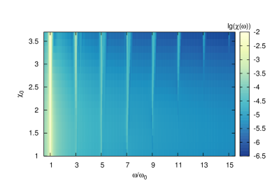
Figure 2: The radiation spectrum via logarithm of the normalized field strength $\chi\left(\omega\right)$ (in arbitrary units) versus pump wave intensity with $\omega_{B}/\omega_{0}=1.5$. The LL broadening is taken to be $\Gamma=0.2\hbar\omega_{B}$.

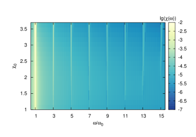
Figure 3: Same as Fig. 2 but for $\omega_{B}/\omega_{0}=2$.

We further examine emission strengths of the 3rd, 5th, 7th, and 9th harmonics for various pump wave frequencies and LL broadening at the fixed value $\chi_{0}=4$, which is shown in Fig. 4. We can see from Fig. 4 that, while the density of states broadens with a width $\sim\Gamma$ the harmonics radiation rates are relatively robust and are feasible up to large $\Gamma$. Then, we see that emission of harmonics takes place for the wide range of the pump wave frequencies.

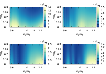
Figure 4: Harmonic emission rate in Landau-quantized graphene at the multiphoton excitation via $\chi_{n}\equiv\chi\left(n\omega_{0}\right)$ for 3rd, 5th, 7th, and 9th harmonics versus LL broadening and pump wave frequency (ratio $\omega_{B}/\omega$) for a wave of intensity $\chi_{0}=4$.

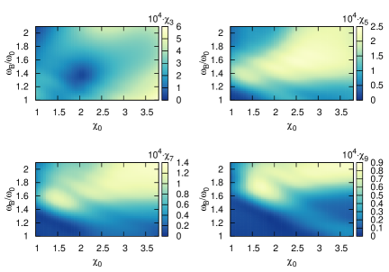
Figure 5: Harmonic emission rate in Landau-quantized graphene at the multiphoton excitation via $\chi_{n}\equiv\chi\left(n\omega_{0}\right)$ for 3rd, 5th, 7th, and 9th harmonics versus pump wave frequency (ratio $\omega_{B}/\omega$) and intensity parameter $\chi_{0}$. The LL broadening is taken to be $\Gamma=0.2\hbar\omega_{B}$.

We also examine how the emission strengths of the 3rd, 5th, 7th, and 9th harmonics behave depending on the pump wave intensity and frequency at the fixed value of LL broadening. The results of our calculations are shown in Fig. (5). Thus, at $\chi_{0}\succsim 1$ we have intense radiation of harmonics and optimal frequencies for pump wave are close to $\omega_{B}/\omega_{0}\approx 2$.

IV SUMMARY

To summarize, we have presented a microscopic theory of the Landau-quantized graphene interaction with coherent electromagnetic radiation towards high harmonics generation. We have shown that the nonlinear optical response of Landau-quantized graphene is quite large that persist for a wide range of the pump wave frequencies and intensities $\chi_{0}>1$ even for significant broadening of  LLs because of impurities in graphene.

Let us consider the experimental feasibility of considered process. For the pump wave field we will assume a $\mathrm{CO}_{2}$ laser with $\hbar\omega\simeq 0.1\ \mathrm{eV}$. For the magnetic field we take $B=40\ \mathrm{T}$. The average intensity of the wave for $\chi_{0}=3$ is $I_{0}\simeq 7\times 10^{8}$ $\mathrm{W/cm}^{2}$. It is clear that for the experimental realization one needs multilayer epitaxial graphene epi . We consider experimentally achievable values $N_{L}\sim 50$ monolayers Layers with the film thickness $\sim 20$ $\mathrm{nm}$. Since film thickness is much smaller than the considered wavelengths, the harmonics’ signal from all layers will sum up constructively. Thus, for the average intensities of the harmonics we will have $I_{s}\simeq I_{0}N_{L}^{2}\chi_{s}^{2}/\chi_{0}^{2}$. For the setup of Fig. 5 with the chosen parameters the average intensities of the harmonics are estimated to be $I_{3}=7.2\times 10^{4}\ \mathrm{W/cm}^{2}$, $I_{5}=1.2\times 10^{4}\ \mathrm{W/cm}^{2}$, $I_{7}=4\times 10^{3}$ $\mathrm{W/cm}^{2}$, and $I_{9}\simeq 1.6\times 10^{3}$ $\mathrm{W/cm}^{2}$.

- (1) K. S. Novoselov, A. K. Geim, S. V. Morozov, D. Jiang, Y. Zhang, S. V. Dubonos, I. V. Grigorieva, and A. A. Firsov, “Electric field effect in atomically thin carbon films”, Science 306(5696), 666–669 (2004), http://dx.doi.org/10.1126/science.1102896.
- (2) A. H. Castro Neto, F. Guinea, N. M. R. Peres, K. S. Novoselov, and A. K. Geim, “The electronic properties of graphene”, Rev. Mod. Phys. 81(1), 109–162 (2009), http://dx.doi.org/10.1103/RevModPhys.81.109.
- (3) S. A. Mikhailov, “Non-linear electromagnetic response of graphene,” Europhys. Lett. 79(2), 27002 (2007), http://dx.doi.org/10.1209/0295-5075/79/27002.
- (4) S. A. Mikhailov and K. Ziegler, “Nonlinear electromagnetic response of graphene: frequency multiplication and the self-consistent-field effects,” J. Phys. Condens. Matter. 20(38), 384204 (2008), http://dx.doi.org/10.1088/0953-8984/20/38/384204.
- (5) F. J. Lopez-Rodriguez and G. G. Naumis, “Analytic solution for electrons and holes in graphene under electromagnetic waves: gap appearance and nonlinear effects,” Phys. Rev. B 78(20), 201406(R) (2008), http://dx.doi.org/10.1103/PhysRevB.78.201406.
- (6) K. L. Ishikawa, “Nonlinear optical response of graphene in time domain,” Phys. Rev. B 82(20), 201402(R) (2010), http://dx.doi.org/10.1103/PhysRevB.82.201402.
- (7) M. M. Glazov, “Second harmonic generation in graphene,” JETP Lett. 93(7), 366–371 (2011), http://dx.doi.org/10.1134/S0021364011070046.
- (8) H. K. Avetissian, A. K. Avetissian, G. F. Mkrtchian, Kh. V. Sedrakian, “Creation of particle-hole superposition states in graphene at multiphoton resonant excitation by laser radiation”, Phys. Rev. B 85(11), 115443(1)-115443(10) (2012), http://dx.doi.org/10.1103/PhysRevB.85.115443.
- (9) H. K. Avetissian, A. K. Avetissian, G. F. Mkrtchian, Kh. V. Sedrakian, “Multiphoton resonant excitation of Fermi-Dirac sea in graphene at the interaction with strong laser fields”, J. Nanophoton 6, 061702(1)- 061702(17) (2012), http://dx.doi.org/10.1117/1.JNP.6.061702.
- (10) H. K. Avetissian, G. F. Mkrtchian, K. G. Batrakov, S. A. Maksimenko, A. Hoffmann, “Nonlinear theory of graphene interaction with strong laser radiation beyond the Dirac cone approximation: Coherent control of quantum states in nano-optics”, Phys. Rev. B 88, 245411(1)- 245411(7) (2013), http://dx.doi.org/10.1103/PhysRevB.88.245411.
- (11) H. K. Avetissian, G. F. Mkrtchian, K. G. Batrakov, S. A. Maksimenko, A. Hoffmann, “Multiphoton resonant excitations and high-harmonic generation in bilayer grapheme”, Phys. Rev. B. 88, 165411(1)- 165411(9) (2013), http://dx.doi.org/10.1103/PhysRevB.88.165411.
- (12) K. S. Novoselov et al., “Two-dimensional gas of massless Dirac fermions in graphene”, Nature 438, 197–200 (2005), http://dx.doi.org/10.1038/nature04233.
- (13) Y. Zhang et al., “Experimental observation of the quantum Hall effect and Berry’s phase in graphene”, Nature 438, 201-204 (2005), http://dx.doi.org/10.1038/nature04235.
- (14) V. P. Gusynin and S. G. Sharapov, “Unconventional integer quantum Hall effect in graphene”, Phys. Rev. Lett. 95, 146801(1)-146801(4) (2005), http://dx.doi.org/10.1103/PhysRevLett.95.146801.
- (15) M. O. Goerbig, ”Electronic properties of graphene in a strong magnetic field”, Rev. Mod. Phys. 83, 1193-1243 (2011), http://dx.doi.org/10.1103/RevModPhys.83.1193.
- (16) T. Morimoto, Y. Hatsugai, and H. Aoki, “Optical Hall conductivity in ordinary and graphene quantum Hall systems”, Phys. Rev. Lett. 103, 116803(1)-116803(4) (2009), http://dx.doi.org/10.1103/PhysRevLett.103.116803.
- (17) N. M. R. Peres, F. Guinea, and A. H. Castro Neto, “Electronic properties of disordered two-dimensional carbon”, Phys. Rev. B 73, 125411(1)-125411(23) (2006), http://dx.doi.org/10.1103/PhysRevB.73.125411.
- (18) V. P. Gusynin, S. G. Sharapov, and J. P. Carbotte, “Anomalous absorption line in the magneto-optical response of graphene”, Phys. Rev. Lett. 98, 157402(1)-157402(4) (2007), http://dx.doi.org/10.1103/PhysRevLett.98.157402.
- (19) C. Zhang, L. Chen, and Z. S. Ma, “Orientation dependence of the optical spectra in graphene at high frequencies”, Phys. Rev. B 77, 241402(1)-241402(4) (2008), http://dx.doi.org/10.1103/PhysRevB.77.241402.
- (20) C. H. Yang, F. M. Peeters, and W. Xu, “Density of states and magneto-optical conductivity of graphene in a perpendicular magnetic field”, Phys. Rev. B 82, 205428(1)-205428(8) (2010), http://dx.doi.org/10.1103/PhysRevB.82.205428.
- (21) T. Morimoto, Y. Hatsugai, and H. Aoki, “Cyclotron radiation and emission in graphene”, Phys. Rev. B 78, 073406(1)-073406(4) (2008), http://dx.doi.org/10.1103/PhysRevB.78.073406.
- (22) A. Ferreira, J. Viana-Gomes, Yu. V. Bludov, V. Pereira, N. M. R. Peres, and A. H. Castro Neto, “Faraday effect in graphene enclosed in an optical cavity and the equation of motion method for the study of magneto-optical transport in solids”, Phys. Rev. B 84, 235410(1)-235410(25) (2011), http://dx.doi.org/10.1103/PhysRevB.84.235410.
- (23) F. Wendler, A. Knorr, E. Malic, “Carrier multiplication in graphene under Landau quantization”, Nature Commun. 5, 3703(1)-3703(6) (2014), http://dx.doi.org/10.1038/ncomms4703.
- (24) F. Wendler, A. Knorr, E. Malic, “Ultrafast carrier dynamics in Landau-quantized graphene”, Nanophotonics 4, 224–249 (2015), http://dx.doi.org/10.1515/nanoph-2015-0018.
- (25) F. Wendler, E. Malic, “Towards a tunable graphene-based Landau level laser in the terahertz regime”, Scientific Reports 5, 12646 (2015), http://dx.doi.org/10.1038/srep12646.
- (26) H. K. Avetissian, G. F. Mkrtchian, “Coherent nonlinear optical response of graphene in the quantum Hall regime”, Phys. Rev. B 94(4), 045419(1)-045419(7) (2016), http://dx.doi.org/10.1103/PhysRevB.94.045419.
- (27) H. K. Avetissian, G. F. Mkrtchian, “Nonlinear response of the quantum Hall system to a strong electromagnetic radiation”, Phys. Lett. A 380(46), 3924–3927 (2016), http://dx.doi.org/10.1016/j.physleta.2016.09.024.
- (28) N. H. Shon and T. Ando, ”Quantum Transport in Two-Dimensional Graphite System”, J. Phys. Soc. Jpn. 67, 2421–2429 (1998), http://dx.doi.org/10.1143/JPSJ.67.2421.
- (29) C. Berger, Z. Song, X. Li, X. Wu, N. Brown, C. Naud, D. Mayou, T. Li, J. Hass, A. N. Marchenkov, E. H. Conrad, P. N. First, and W. A. de Heer, “Electronic Confinement and Coherence in Patterned Epitaxial Graphene”, Science 312(5777), 1191-1196 (2006), http://dx.doi.org/10.1126/science.1125925.
- (30) A.L. Friedman, J.L.Tedesco, P.M.Campbell, J.C. Culbertson, E. Aifer, F.K. Perkins, R.L. Myers-Ward, J.K.Hite , C.R. Eddy Jr, G.G.Jernigan, and D.K. Gaskill, “Quantum linear magnetoresistance in multilayer epitaxial graphene”, Nano letters, 10(10), 3962-3965, (2010), http://dx.doi.org/10.1021/nl101797d.