Abstract

As part of an effort to better characterize bright cataclysmic variables (CVs) which have received little attention in the past light curves of four confirmed systems (CZ Aql, BO Cet, V380 Oph and EF Tuc) and one candidate (Lib 3) are analyzed. For none of these stars time resolved photometry has been published previously. While no variability was found in the case of Lib 3, which thus cannot be confirmed as a CV, the light curves of all other targets are dominated by strong flickering. Modulations on hourly time scales superimposed on the flickering can probably be related to orbital variations in BO Cet and V380 Oph, but not in CZ Aql and EF Tuc. Variations on the time scale of 10 minutes in CZ Aql, while not yet constituting convincing evidence, together with previous suspicions of a magnetically channeled accretion flow may point at an intermediate polar nature of this star. Some properties of the flickering are quantified in an effort to enlarge the data base for future comparative flickering studies in CVs and to refine the classification of the target stars.

Keywords: Stars: novae, cataclysmic variables – Stars: individual: CZ Aql – Stars: individual: BO Cet – Stars: individual: V380 Oph – Stars: individual: EF Tuc – Stars: individual: Lib 3

1 Introduction

Cataclysmic variables (CVs) are binary stars where a Roche-lobe filling late-type component (the secondary) transfers matter via an accretion disk to a white dwarf primary. It may be surprising that even after decades of intense studies of CVs there are still an appreciable number of known or suspected systems, bright enough to be easily observed with comparatively small telescopes, which have not been studied sufficiently for basic parameters such as the orbital period to be known with certainty. In some cases even their very class membership is not confirmed.

Therefore, I started a small observing project aimed at a better understanding of these so far neglected stars. First results have been published in Bruch (2016) and Bruch (2017). Here, I discuss light curves of some further targets of the project for which no time resolved photometry has yet been published. They were observed in order to verify the presence of flickering typically observed in CVs and to try to measure the orbital period photometrically (or to confirm suspected periods).

It is well known that accretion of mass via a disk onto a central object normally leads to apparently stochastic brightness variations termed flickering. It occurs to a more or less obvious degree in objects as diverse as Active Galactic Nuclei (Garcia et al. 1999), certain stages of star formation (Herbst & Sevchenko 1999, Kenyon et al. 2000, Scaringi et al 2015), x-ray binaries (van der Klis 2004) or some (but not all) symbiotic stars (Gromadzki et al. 2006). The time scales of such variations and the spectral range in which they most prominently appear depend on the nature of the particular system. In the optical range flickering is by far most conspicuous in CVs where it leads to variability typically on time scales of the order of minutes and with amplitudes which can range from a few millimagnitudes to more than an entire magnitude. For a general characterization of flickering in CVs, see Bruch (1992).

While the strength of the flickering, as measured by its total amplitude, depends heavily on the individual system and its momentary photometric state no photometric observations of well established CVs obtained with a suitable time resolution and signal-to-noise ratio, of which the present author is aware, ever showed the absence of flickering, unless the respective system was in a state of (temporary) suspension of mass accretion onto the white dwarf. Thus, the presence of flickering appears to be a necessary (but not sufficient) condition for a star to be classified as a cataclysmic variable.

While flickering by itself is a fascinating and still not well understood phenomenon, it can also be a severe obstacle to find and characterize modes of variability in CVs which may have similar amplitudes but are due to different mechanisms. Thus, orbital variations caused by the changing aspect of the system around the orbit may easily be masked by flickering. This is the case in particular in systems with a low or intermediate orbital inclination where such variations remain small and in the presence of flickering may only be detected when observations over many cycles are averaged.

The objects discussed in the present paper are four systems taken from the most recent on-line version of the Ritter & Kolb catalogue [Ritter03] which have only unconfirmed or uncertain orbital periods. These are CZ Aql, BO Cet, V380 Oph and EF Tuc. To these I add Lib 3 (= Preston 874124), an unconfirmed CV listed in the catalogue of Downes et al. 2005 and classified as being of UX UMa subtype.

In Sect. 2 the observations and data reduction techniques are briefly presented. Sects. 3 – 7 deal with the individual objects of this study, focusing on orbital variations, while in Sect. 8 the rapid variations observed in four of the five targets are collectively quantified. Finally, a short summary in Sect. 9 concludes this paper.

2 Observations and data reductions

All observations were obtained at the 0.6-m Zeiss and the 0.6-m Boller & Chivens telescopes of the Observatório do Pico dos Dias, operated by the Laboratório Nacional de Astrofísica, Brazil. Time series imaging of the field around the target stars was performed using cameras of type Andor iKon-L936-B and iKon-L936-EX2 equipped with back illuminated, visually optimized CCDs. In order to resolve the expected rapid flickering variations the integration times were kept short. Together with the small readout times of the detectors this resulted in a time resolution of the order of 5${}^{\raisebox{0.90417pt}{\scriptsize s}}$. In order to maximize the count rates in these short time intervals no filters were used. Therefore, it was not possible to calibrate the stellar magnitudes. Instead, the brightness is expressed as the magnitude difference between the target and a nearby comparison star. This is not a severe limitation in view of the purpose to the observations. A rough estimate of the effective wavelength of the white light band pass, assuming a mean atmospheric extinction curve, a flat transmission curve for the telescope, and a detector efficiency curve as provided by the manufacturer, yields $\lambda_{\rm eff}\approx 5530\AA$, very close to the effective wavelength of the Johnson $V$ band (5500 Å; Allen 1973).

A summary of the observations is given in Table 1. Some light curves contain gaps caused by intermittent clouds or technical reasons. Basic data reduction (biasing, flat-fielding) was performed using IRAF. For the construction of light curves aperture photometry routines implemented in the MIRA software system (Bruch 1993) were employed. The same system was used for all further data reductions and calculations. Throughout this paper time is expressed in UT. However, whenever observations taken in different nights were combined (e.g., to search for orbital variations) time was transformed into barycentric Julian Date on the Barycentric Dynamical Time (TDB) scale using the online tool provided by Eastman et al. (2010) in order to take into account variations of the light travel time within the solar system. Timing analysis of the data employing Fourier techniques was done using the Lomb-Scargle algorithm (Lomb 1976, Scargle 1982, Horne & Baliunas 1986) unless specified otherwise. The terms “power spectrum” and “Lomb-Scargle periodogram” are used synonymously for the resulting graphs.

Table 1: Journal of observations

Name	Date	Start	End
		(UT)	(UT)
CZ Aql	2014 Jun 17	23:31	28:54
	2014 Jun 19	22:40	28:31
	2014 Aug 25/26	22:46	24:06
	2014 Sep 21/22	22:16	22:28
	2014 Sep 22	21:44	23:12
	2014 Sep 23	21:47	23:13
	2014 Sep 24	21:56	23:22
BO Cet	2014 Sep 23	25:21	28:14
	2014 Sep 24	25:12	28:10
	2014 Oct 23	21:31	23:10
	2016 Aug 11	25:49	28:51
	2016 Aug 12	25:55	28:44
Lib 3	2016 Jun 27/28	21:16	2:55
V380 Oph	2014 Jun 18	21:00	26:37
	2014 Jun 20	24:36	26:05
	2014 Jun 22	22:37	24:30
EF Tuc	2014 Jun 18	28:02	28:44
	2014 Jun 23	24:06	28:56
	2014 Aug 26	24:50	28:43
	2014 Sep 22	22:39	28:13
	2014 Sep 22/23	23:20	25:11
	2014 Sep 23/24	23:22	25:05
	2014 Sep 24/25	23:27	22:19
	2015 Aug 11	27:40	28:47
	2015 Aug 12	27:18	28:41
	2015 Aug 13	26:52	28:51
	2015 Aug 14	27:06	28:59
	2015 Aug 15	27:01	28:41

3 CZ Aql

CZ Aql was discovered as a variable star by Reinmuth (1925) who did not provide a classification. Based on spectroscopic evidence, Cieslinski et al. (1998) considered the star to be a dwarf nova and suspected an orbital period of 4.8 hours. This is confirmed by Sheets et al. (2007) who find $P_{\rm orb}=0.2005$ days = 4.812 hours but cannot distinguish between aliases ranging between 4.798 and 4.826 hours. Based on a detailed spectroscopic analysis they suspect CZ Aql to contain a magnetically channeled accretion flow.

CZ Aql was observed in seven nights between 2014, June 17 and September 24. Representative light curves, drawn on the same time and magnitude scale to ease comparison, are shown in Fig. 1. Differential magnitudes are given with respect to the comparison star UCAC4 415-122382 ($V=14\mbox{${}^{\raisebox{0.90417pt}{\scriptsize m}}_{\raisebox{1.80835pt}{\hskip 1.18999pt.}}$}122$; Zacharias et al. 2013). This translates into a rough average nightly magnitude of CZ Aql between $15\mbox{${}^{\raisebox{0.90417pt}{\scriptsize m}}_{\raisebox{1.80835pt}{\hskip 1.18999pt.}}$}0$ and $15\mbox{${}^{\raisebox{0.90417pt}{\scriptsize m}}_{\raisebox{1.80835pt}{\hskip 1.18999pt.}}$}3$ which is on the faint end of the distribution of the few magnitude estimates in the data base of the American Association of Variable Star Observers (AAVSO).

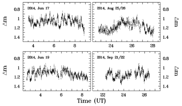
Figure 1: Light curves of CZ Aql observed in four nights in 2014.

The light curves are dominated by flickering superposed on more gradual variations on the time scale of several hours, most clearly visible on 2014, Aug. 25 (Fig. 1). In fact, adjusting a sine curve to the data of that night alone gives a best fit at a period of 4.704 hours, just slightly shorter than but still compatible with the spectroscopic period determined by Sheets et al. (2007). In order to investigate if the variations can be explained as a periodic modulation all light curves were combined into a single data set after subtracting the mean differential magnitude of the individual nights in order to remove long term brightness changes. The final part of the light curve of 2014 June 17 (Fig. 1) was not considered since the sudden drop observed at the very end may in part be due to colour differences between CZ Aql and the comparison star, the observations having been performed at an air mass $>2$.

A power spectrum of the combined light curve was calculated (upper frame of Fig. 2). Due to the distribution of the light curves along three months, it contains strong alias patterns with a broad maximum roughly consistent with the spectroscopic period. However, none of the alias peaks coincides with that period (marked by the red vertical line in the figure) or lies within the possible range quoted by Sheets et al. (2007). Instead, the frequency of the strongest peak corresponds to a period of 5.2083 hours, $\sim$8% longer than the orbital period. Folding the combined light curves on this period (lower frame of Fig. 2) results in a consistent, approximately sinusoidal pattern, modulated on small scales in phase by the strong flickering of the star. But note that the light curve folded on periods corresponding to other peaks in the power spectrum exhibit very similar patterns.

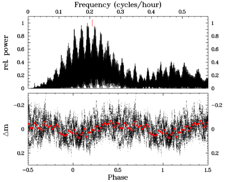
Figure 2: Top: Power spectrum of the combined light curves of CZ Aql of 2014, June 17 and 19. The red vertical line marks the spectroscopic period. Bottom: Light curves folded on the period $P=5.2083$ hours, corresponding to the highest peak in the power spectrum. The red dots represent a binned version of the folded light curve.

While the folded light curve thus suggests consistent variations of CZ Aql over a time scale of several months, it would be premature to consider them firmly established. Similar variations with periods not coinciding with the orbital period have been observed in other cataclysmic variables and have shown not be to stable on longer time scales. Examples include V603 Aql (Haefner & Metz 1985, Bruch 1991, Patterson et al. 1993), TT Ari (Belova et al. 2013 and references therein; Smak 2013), KR Aur (Kozhevnikov 2007), V751 Cyg (Patterson et al. 2001, Papadaki et al. 2009), V795 Her (Papadaki et al. 2006), and V378 Peg (Kozhevnikov 2012). Such variations are often interpreted as positive or negative superhumps. Long light curves observed during subsequent nights should permit to verify if the variability of CZ Aql follows similar patterns.

4 BO Cet

BO Cet is first mentioned as a variable star and classified as a novalike variable in the 71th name list of variable stars (Kazarovetz et al. 1993) with a reference to a manuscript by R. Remillard. Similarly, in the on-line edition of their catalog and atlas of cataclysmic variables Downes et al. (2005) cite a private communication of R. Remillard as type reference for the star.

There is no doubt about the nature of BO Cet as a cataclysmic variable. The colours measured by Zwitter & Munari (1995) ($U-B=-0.7$; $B-V=0.1$; $V-R=0.07$; $R-I=0.10$) are quite normal for a CV where the contribution of the secondary star is negligible. The same authors also reproduce a spectrum of the star which exhibits a strong blue continuum superposed by hydrogen and He I emission lines. Moreover, a rather strong He II $\lambda$ 4686 Å  emission is also present, reaching an integrated flux similar to that of H$\delta$. Based on time resolved spectroscopic observations Rodríguez-Gil et al. (2007) classified BO Cen as a SW Sextantis type star. The orbital period of 0.13980 $\pm$ 0.00006 days (3${}^{\raisebox{0.90417pt}{\scriptsize h}}_{\raisebox{1.80835pt}{\hskip 1.18999pt.}}$3552) is only known from an informal communication by J.  Patterson based on Center for Backyard Astrophysics (CBA) data.

Since the CBA observations are not otherwise documented I retrieved the light curve of BO Cet from Patterson’s communication. Phase Dispersion Minimization (Stellingwerf 1978) as well as Analysis of Variance (Schwarzenberg-Czerny 1989), of these data, both better suited for period searches in non-sinusoidally varying signals than Fourier transforms, yield a slightly longer period (but still comfortably within the error limits) of $P_{\rm orb}=0.13983$ days than that informed by Patterson. The difference implies a phase shift of 0.05 over the time base of the CBA observations. Therefore, the phase folded light curve, reproduced in Fig. 3 is slightly different (in fact, “nicer”, particularly at the primary minimum) than the one based on Patterson’s period. If the phase of the secondary minimum, interpreted by Patterson as a shallow eclipse, is defined as phase $\phi=0$, the average light curve assumes a minimum (deeper than the eclipse) at $\phi=0.75$, rises steeply until $\phi=0.1$ (this rise being interrupted by the eclipse) and then declines first slowly and then more rapidly after $\phi=0.5$. This waveform is different from the orbital variations of most CVs which often (but not always) exhibit a hump caused by a hot spot in the range $0.75\leq\phi\leq 1$.

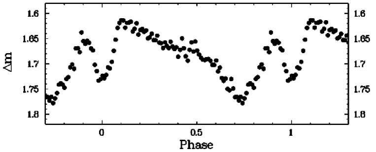
Figure 3: Average orbital light curve of BO Cet based on CBA data.

The absence of published time resolved photometry of BO Cet prompted me to include the star in the present observing project. I observed it in five nights in 2014 and 2016 (see Table 1), obtaining light curves with durations of the order of 3${}^{\raisebox{0.90417pt}{\scriptsize h}}$ (1${}^{\raisebox{0.90417pt}{\scriptsize h}}$ in one case) which is close to the reported orbital period. They are shown (all drawn on the same time and magnitude scale in order to ease comparison) in Fig. 4. Differential magnitudes are given with respect to the comparison star UCAC4 441-002697 ($V=12\mbox{${}^{\raisebox{0.90417pt}{\scriptsize m}}_{\raisebox{1.80835pt}{\hskip 1.18999pt.}}$}720$; Zacharias et al. 2013). The average nightly magnitudes of BO Cet thus varied roughly between $14\mbox{${}^{\raisebox{0.90417pt}{\scriptsize m}}_{\raisebox{1.80835pt}{\hskip 1.18999pt.}}$}5$ and $14\mbox{${}^{\raisebox{0.90417pt}{\scriptsize m}}_{\raisebox{1.80835pt}{\hskip 1.18999pt.}}$}7$, well within the brightness range quoted in the data base of the the Association Française des Observateurs d’Etoiles Variables (AFOEV; 13${}^{\raisebox{0.90417pt}{\scriptsize m}}_{\raisebox{1.80835pt}{\hskip 1.18999pt.}}$6 – 15${}^{\raisebox{0.90417pt}{\scriptsize m}}_{\raisebox{1.80835pt}{\hskip 1.18999pt.}}$2) and the British Astronomical Association, Variable Star Section (BAAVSS; 14${}^{\raisebox{0.90417pt}{\scriptsize m}}_{\raisebox{1.80835pt}{\hskip 1.18999pt.}}$3 – 14${}^{\raisebox{0.90417pt}{\scriptsize m}}_{\raisebox{1.80835pt}{\hskip 1.18999pt.}}$).

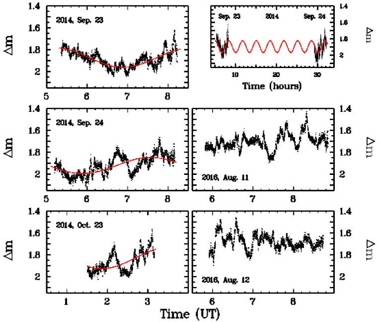
Figure 4: Light curves of BO Cet observed in 2014 (frames on the left side) and 2016 (lower two frame on the right side). The red curves are sine fits to the data, where the period has been fixed to $P_{\rm orb}$. The upper right frame contains the combined light curves of 2015, Sep. 24 and 25 together with the best fit sine curve, showing that the adopted period does not lead to a significant phase shift between the data of the two nights.

BO Cet is characterized by significant flickering as is normal for cataclysmic variables. Moreover, the light curves observed in 2014 exhibit more gradual variations which are compatible with a modulation on the orbital period. This is highlighted in the figure by the red curves which are best sine fits to the data (as a rough approximation to the orbital variations) where the period has been fixed to $P_{\rm orb}$. The amplitude of this modulation, measured to be 0${}^{\raisebox{0.90417pt}{\scriptsize m}}_{\raisebox{1.80835pt}{\hskip 1.18999pt.}}$089 (0${}^{\raisebox{0.90417pt}{\scriptsize m}}_{\raisebox{1.80835pt}{\hskip 1.18999pt.}}$074; 0${}^{\raisebox{0.90417pt}{\scriptsize m}}_{\raisebox{1.80835pt}{\hskip 1.18999pt.}}$095) on 2016, Sep. 23 (Sep. 24, Oct. 23), may be considered constant regarding the uncertainties expected in view of the flickering activity.

The upper right frame of Fig. 4 shows the combined light curves observed on 2014, Sep. 23 and 24 together with the best fit sine curve, again with the period fixed to $P_{\rm orb}$. While the variations on Sep. 24 are not perfectly in phase with those of the previous night the difference is not large enough to suggest a significant period error, again considering the strong flickering.

Compared to 2014, in the 2016 observations the orbital modulation is not as well expressed. The overall magnitude level being slightly higher may not be significant since different detectors were used during the two epochs which introduces uncertainties in the differential magnitudes of these uncalibrated white light measurements.

5 V380 Oph

V380 Oph was identified as a variable star by Hoffmeister (1929). Its spectrum is considered as a “textbook example” for a CV by Liu et al. (1999b). X-rays from the source were detected in the ROSAT All Sky Survey (Verbunt et al. 1997).

The orbital period was spectroscopically determined by Shafter (1983, 1985) to be 0.16 days; a value later refined to 0.154107 days (3.6986 hours) by Rodríguez-Gil et al. (2007) who also classified V380 Oph as a SW Sex star. A long-term light curve with rather smooth variations between $\sim$$14\mbox{${}^{\raisebox{0.90417pt}{\scriptsize m}}_{\raisebox{1.80835pt}{\hskip 1.18999pt.}}$}3$ and $16\mbox{${}^{\raisebox{0.90417pt}{\scriptsize m}}$}$ is shown by Kafka & Honeycutt (2004), but an excursion to a low state of $\sim$$17\mbox{${}^{\raisebox{0.90417pt}{\scriptsize m}}_{\raisebox{1.80835pt}{\hskip 1.18999pt.}}$}5$ observed by Shugarov et al. (2005) and in particular light curves generated from more recent data provided by the AAVSO, the AFOEV and the BAAVSS also justify to count V380 Oph among the VY Scl stars.

V380 Oph was observed in the three nights of 2014 June 18, 20 and 22. The light curves, expressed as differential magnitudes with respect to the primary comparison star UCAC4 481-069940 are shown in Fig. 5. This star having a magnitude of $V=13\mbox{${}^{\raisebox{0.90417pt}{\scriptsize m}}_{\raisebox{1.80835pt}{\hskip 1.18999pt.}}$}911$ (Zacharias et al. 2013), a mean brightness of V380 Oph of roughly 15${}^{\raisebox{0.90417pt}{\scriptsize m}}_{\raisebox{1.80835pt}{\hskip 1.18999pt.}}$4 with only slight night-to-night variations is calculated. This is slightly fainter than the average brightness of the system according to Kafka & Honeycutt (2004) and the long term light curves found in the AAVSO, AFOEV and BAAVSS data bases (not considering low states).

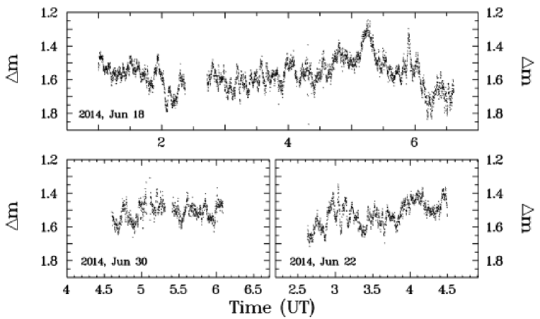
Figure 5: Light curves of V380 Oph during three nights in 2014 June.

The light curves are characterized by significant flickering activity, superposed on variations on hourly time scales. In order to investigate if the latter are compatible with the orbital period, the three light curves were combined into a single data set (without subtracting the average nightly magnitude) and subjected to a Fourier analysis. The low frequency part of the power spectrum is shown in the upper frame of Fig. 6. Overlaid upon the expected alias pattern due to the separation of two nights between the individual light curve segments is a low frequency signal which is roughly compatible with the orbital period determined by Rodríguez-Gil et al. (2007). The frequency corresponding to that period is indicated by a broken vertical line in the figure. While it does not coincide with the highest alias peak it is well aligned with a secondary maximum. Folding the combined light curves on the orbital period (lower frame of Fig. 6) suggests that the brightness variations on hourly time scales have indeed an orbital origin.

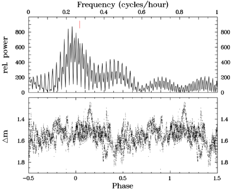
Figure 6: Top: Power spectrum of the combined light curves of V380 Oph on 2014, June 18, 20 and 22. The red vertical line marks the orbital frequency. Bottom: Combined light curve folded on the orbital period.

6 EF Tuc

EF Tuc was discovered as a dwarf nova in the Edinburgh-Cape Blue Object Survey. The spectrum shown by Stobie et al. (1995) is dominated by strong hydrogen emission lines. Chen et al. (2001) investigated the spectrum in somewhat more detail and suspected a SU UMa type classification. They could not measure the orbital period spectroscopically, probably because of a low orbital inclination. The orbital period of 3.6 hours quoted in the Ritter & Kolb catalogue is based on informal communications by J. Patterson in 2003 and 2006 where it is classified as a candidate period. It has never been confirmed. It would contradict the SU UMa classification because stars of that type have periods below the 2.2 – 2.8 hour period gap in the CV orbital period distribution. Chen et al. (2001) also mention time resolved photometry and found that EF Tuc exhibits strong flickering, but they do not show a light curve.

The AAVSO long term light curve, shown in Fig. 7, although not having a dense temporal coverage, exhibits a the typical dwarf nova behaviour with outbursts reaching $\sim$$12\mbox{${}^{\raisebox{0.90417pt}{\scriptsize m}}$}-12\mbox{${}^{\raisebox{0.90417pt}{\scriptsize m}}_{\raisebox{1.80835pt}{\hskip 1.18999pt.}}$}5$ and a quiescent level between 14${}^{\raisebox{0.90417pt}{\scriptsize m}}_{\raisebox{1.80835pt}{\hskip 1.18999pt.}}$5 and 15${}^{\raisebox{0.90417pt}{\scriptsize m}}$. While the coverage is insufficient to verify if some of the outbursts discernable in the figure are superoutbursts or not, their amplitudes are certainly quite low for such an interpretation. The outburst with the best coverage, peaking close to JD 2452120, has a total width of $\sim$40 days which is long even for a superoutburst of an SU UMa star (see, e.g., the compilation of Kato et al. 2009). Moreover, unlike observed in superoutbursts, the rise to maximum takes more than 10 days, and there is no plateau phase after maximum. Thus the long term light curve cannot sustain the SU UMa classification of EF Tuc.

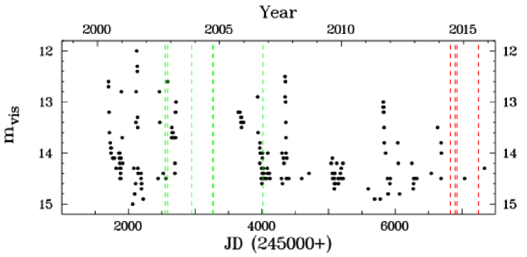
Figure 7: AAVSO long term light curve of EF Tuc. The broken vertical lines indicate the epochs of AAVSO high cadence observations (green) and of the light curves listed in Tab. 1 (red).

EF Tuc was observed in 12 nights in 2014 and 2015. The respective epochs are marked by red vertical lines in Fig. 7. The best data consist of light curves obtained in four consecutive nights in 2014, September. They are shown in Fig. 8 on the same time and magnitude scale. Differential magnitudes are given with respect to the primary comparison star UCAC4 115-000029 ($V=13\mbox{${}^{\raisebox{0.90417pt}{\scriptsize m}}_{\raisebox{1.80835pt}{\hskip 1.18999pt.}}$}328$; Zacharias et al. 2013). The range of average nightly magnitudes of EF Tuc is then 14${}^{\raisebox{0.90417pt}{\scriptsize m}}_{\raisebox{1.80835pt}{\hskip 1.18999pt.}}$5 – 15${}^{\raisebox{0.90417pt}{\scriptsize m}}_{\raisebox{1.80835pt}{\hskip 1.18999pt.}}$4. This is at the faint end of the magnitude distribution in the AAVSO long-term light curves (Fig. 7).

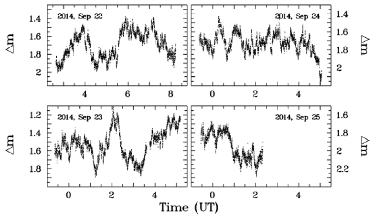
Figure 8: Light curves of EF Tuc in four nights in 2014, September.

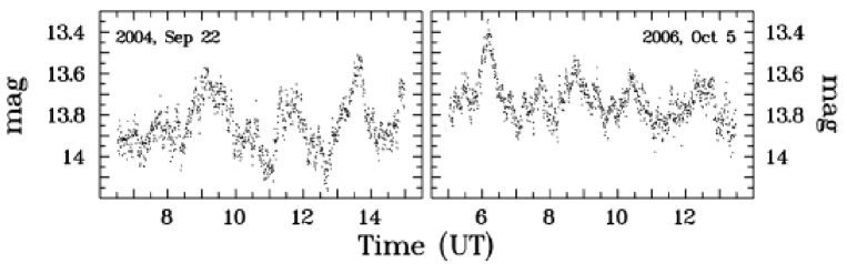
Figure 9: AAVSO high cadence light curves of EF Tuc of 2005, Sep 22 and 2006, Oct. 5.

The light curves are dominated by strong flickering which is superposed on variations occurring on hourly time scales. The total amplitude observed in a single light curve reaches 1${}^{\raisebox{0.90417pt}{\scriptsize m}}_{\raisebox{1.80835pt}{\hskip 1.18999pt.}}$0. On average it is 0${}^{\raisebox{0.90417pt}{\scriptsize m}}_{\raisebox{1.80835pt}{\hskip 1.18999pt.}}$63. Strong variations can occur quite rapidly: On 2014, Jul 23 a drop in magnitude of 0${}^{\raisebox{0.90417pt}{\scriptsize m}}_{\raisebox{1.80835pt}{\hskip 1.18999pt.}}$7 was observed within 35 minutes (see also the strong and rapid flare on 2014, Sep. 23; lower left frame of Fig. 8).

Apart from the long term light curve shown in Fig. 7 the AAVSO archives also contain several high cadence observations (observer: Berto Monard). Although they have a lower time resolution than the other EF Tuc data discussed here they contain complementary information. Therefore, I include them in the present study in particular to perform a search for periodic signals. Details of these light curves are given in Tab. 2. Their epochs are marked by green vertical lines in Fig. 7. Fig. 9 shows two representative examples.

Table 2: High cadence light curves of EF Tuc in the AAVSO data base

Observing	Start	End	Time	Number
Date	(UT)	(UT)	Res. (s)	of Integr.
2002 Oct 21	16:12	11:15	26	1590
2002 Nov 08	15:17	12:37	16	1507
2003 Oct 29	15:10	14:02	60	1259
2003 Nov 07	15:22	12:46	60	1449
2004 Sep 09	17:05	14:45	30	1906
2004 Sep 10	19:08	15:22	31	1402
2004 Sep 15	19:20	15:15	31	1696
2004 Sep 16	17:21	15:05	30	1880
2004 Sep 17	15:42	11:09	30	1629
2004 Sep 19	18:52	14:39	31	1560
2004 Sep 20	11:20	14:57	31	1429
2004 Sep 22	16:31	14:59	31	1999
2004 Sep 26	10:52	15:05	31	1495
2006 Oct 04	16:00	12:51	30	1810
2006 Oct 05	15:02	13:28	30	1999
2006 Oct 06	15:24	16:26	30	1124

In order to search for periodicities on hourly time scales, in particular in order to identify the orbital period of EF Tuc, all light curves were subjected to a power spectrum analysis. Additionally, power spectra of the combined light curves observed within restricted periods of a couple of nights (such as those of 2004, Sep. 9 – 26 or 2015, Sep. 22 – 25) and subsets thereof were calculated. In these cases night-to-night variations of the average magnitude were first subtracted.

The individual light curves are too short to reveal clear periodicities on the time scale of hours; i.e. the range in which the orbital period may be suspected. This is the more so in the presence of strong flickering. However, it is intriguing that most individual power spectra show peaks in the range between 0.35 and 0.45 cycles/hour. In the case of the AAVSO light curves, a second peak centred on 0.15 cycles/hour is often observed, which is missing in the power spectra of the 2014 – 2015 data. The peaks are quite broad due to the limited frequency resolution caused by the finite lengths of the data trains. The power spectra of the combined light curves repeat this pattern, but the peaks are now split up into a many narrow aliases introduced by the complicated window function.

As examples, the summed individual power spectra of the nights of 2004, Sep. 15 – 22 (green) and of 2014, Sep 22 – 24 (red) are shown in the upper frame of Fig. 10. The lower frame of the figure contains the power spectra of the combined light curves in the respective time intervals. Reflecting the trends already seen in the nightly power spectra, in 2004 two almost equally strong clusters of peaks are seen, the highest of which correspond to periods of 5${}^{\raisebox{0.90417pt}{\scriptsize h}}_{\raisebox{1.80835pt}{\hskip 1.18999pt.}}$52 and 2${}^{\raisebox{0.90417pt}{\scriptsize h}}_{\raisebox{1.80835pt}{\hskip 1.18999pt.}}$28, respectively. The low frequency cluster of peaks is absent in the power spectrum of 2014. The much simpler alias pattern, reflecting the smaller number of contributing nightly light curves (resulting in a less complicated window function) is roughly consistent with the higher frequency cluster observed in 2004, but appears to be shifted towards lower frequencies and the individual peaks do not coincide with those of 2004. The highest one in 2015 corresponds to a period of 2${}^{\raisebox{0.90417pt}{\scriptsize h}}_{\raisebox{1.80835pt}{\hskip 1.18999pt.}}$80.

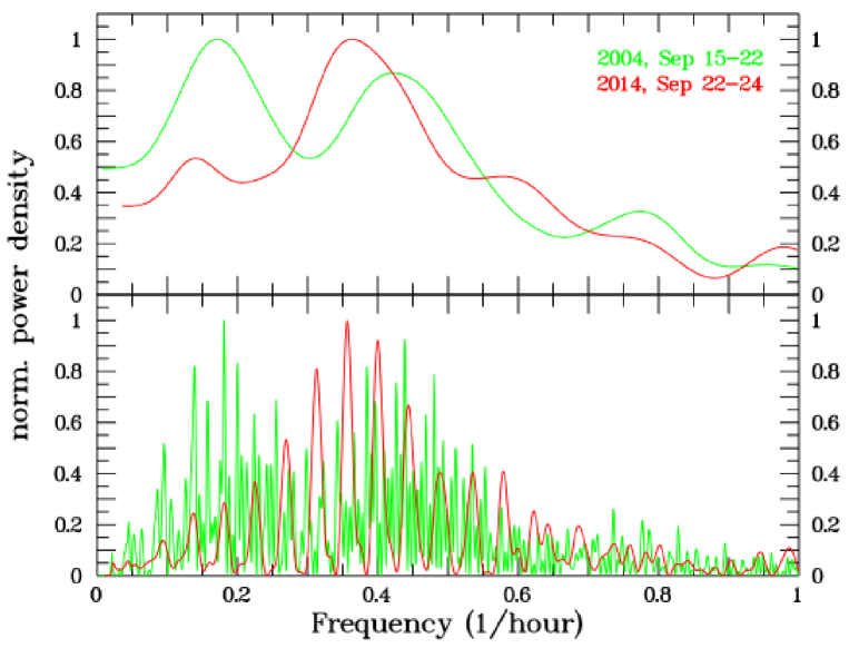
Figure 10: Power spectra of the combined light curves of TF Tuc of 2004, Sep 15-22 (green) and of 2015, Sep. 22-24 (red). For details, see text.

Folding the data on any of the periods does not result in a convincing light curve. The power spectra peaks apparently reflect the presence of decimagnitude variations on the time scales of hours such as those seen on 2014, Sep. 22 and 23 but which are not repeated in other nights such as 2014, Sep. 24 (see Fig. 8). It may therefore be stated that these variations occur on a preferred time scale, but they are not periodic. Thus, the question concerning the orbital period of EF Tuc remains open.

7 Lib 3 = Preston 874124

Lib 3 is quoted as a novalike variable in the catalog of Downes et al. (2005). This classification is based on a private communication of W. Krzeminski cited by Vogt (1989). While this is compatible with the optical colours ($B-V=0.15$; $U-B=-0.91$; Beers et al. 1992) the only published spectrum, showing a blue continuum and weak and broad Balmer absorption lines (Liu et al. 1999a) is inconclusive.

I therefore observed a light curve of Lib 3 extending for about 5${}^{\raisebox{0.90417pt}{\scriptsize h}}_{\raisebox{1.80835pt}{\hskip 1.18999pt.}}$5. During this period the differential magnitude with respect to the primary comparison star UCAC4 299-243578 remained constant within the standard deviation of 0${}^{\raisebox{0.90417pt}{\scriptsize m}}_{\raisebox{1.80835pt}{\hskip 1.18999pt.}}$015 of the individual data points. This complete absence for any sign of flickering during such a long time is a strong indication that Lib 3 is not a cataclysmic variable.

Since the finding chart published by Downes et al. (2005) is based on a coordinate match instead of a positive identification of a variable star a mis-identification cannot be excluded. Therefore, I also measured the differential magnitude with respect to UCAC4 299-243578 of all stars within 5 arc minutes around the primary candidate which are bright enough to be subjected to photometry, considering the limitations of the available data. In no case variability was detected.

8 Variations on short time scales

With the exception of Lib 3 all objects of the present study exhibit rather strong variations on the time scale of minutes. Most of this is expected to be random flickering as is typical in CVs. However, it is always worthwhile to investigate if other than apparently stochastic variations hide beneath the flickering, as is a characterization of the flickering properties themselves. Therefore, some basic parameters of the rapid light curve modulations are determined here. While it is possible to draw some immediate conclusions, they also serve as input for are more systematic quantitative and comparative investigation of the flickering in many cataclysmic variables (Bruch, in preparation).

8.1 Flickering amplitude

One of the basic properties of flickering is its total amplitude. However, if simply taken to be the difference between maximum and minimum magnitude in a light curve, it will depend to a certain extent on the length of the data train: the probability to accidentally observe particularly strong flickering flares is larger in longer light curves than in shorter ones. On the other hand, long light curves may contain variations not related to flickering (i.e., orbital humps).

In order to render a determination of the flickering amplitude comparable between different light curves of the same object and between different objects, I only regard that part of the flickering which occurs on time scales of less than 30${}^{\raisebox{0.90417pt}{\scriptsize m}}$ (much less than the typical length of a light curve). To this end, the original data are smoothed by applying a Fourier filter which effectively removes all variations on a time scale below 30${}^{\raisebox{0.90417pt}{\scriptsize m}}$. The difference of the smoothed and the original version then represents a high pass filtered light curve which is free from variations on longer time scales. Even so the difference between maximum and minimum brightness may still depend strongly on accidental events in the light curve. Therefore, in order to obtain a more “typical” value I take the FWHM of a Gaussian adjusted to the distribution of the individual magnitude values, as a proxy for the flickering amplitude. For each object of the current study the average of the corresponding values determined from all available light curves is listed together with their standard deviation in Table 3. Since data noise tends to broaden the distribution, it still depends on the noise level in the data which, however, is similar in all light curves. Applying the formula provided by Da Costa (1992) the noise in the differential light curves is in all cases estimated to be of the same order of magnitude (0${}^{\raisebox{0.90417pt}{\scriptsize m}}_{\raisebox{1.80835pt}{\hskip 1.18999pt.}}$01), meaning that the numbers in Table 3 are comparable among each other.

Not surprisingly, the flickering amplitude varies significantly from one oject to the other. However, for a given star it remains fairly constant over time.

Table 3: Flickering parameters

Object	Amplitude	$\alpha_{\rm ps}$	$\alpha_{\rm wav}$	$\Sigma$	Number of
Name	(FWHM)(mag)	(power spectrum)	(wavelet)	(wavelet)	light curves
CZ Aql	0.103 $\pm$ 0.019	-1.76 $\pm$ 0.35 (0.13)	1.99 $\pm$ 0.19	-1.22 $\pm$ 0.11	27
BO Cet	0.071 $\pm$ 0.007	-2.06 $\pm$ 0.26 (0.12)	1.82 $\pm$ 0.12	-1.47 $\pm$ 0.09	25
V380 Oph	0.094 $\pm$ 0.002	-1.57 $\pm$ 0.09 (0.05)	1.52 $\pm$ 0.12	-1.31 $\pm$ 0.02	23
EF Tuc	0.117 $\pm$ 0.016	-1.52 $\pm$ 0.36 (0.10)	1.56 $\pm$ 0.30	-1.11 $\pm$ 0.11	12

8.2 Red noise behaviour

On the double logarithmic scale the power spectra of CV light curves exhibit a characteristic shape (see e.g. Bruch 1992). It is more or less constant at low frequencies (somewhat modulated due to stochastic variations occurring on the corresponding long time scales). It then declines linearly to higher frequencies reflecting red noise behaviour and finally levels off to an approximately constant level at very high frequencies due to the dominance of white noise at these scales. As an example, in Fig. 11 the power spectrum of the light curve of BO Cet of 2016, Aug. 11, is shown, calculated up to the Nyquist frequency, at the original sampling frequencies (black points) and binned into frequency intervals of $\Delta\log(f)=0.05$ (red dots).

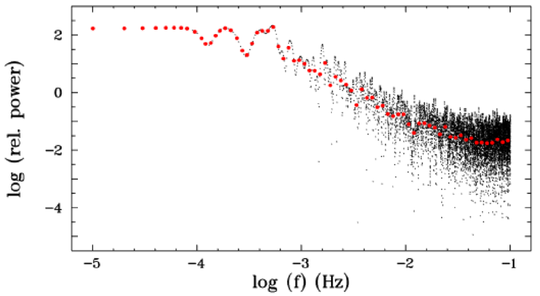
Figure 11: Lomb-Scargle power spectrum of the light curve of BO Cet observed on 2016, Aug. 11 on a double logarithmic scale (black points). The red dots show the same data, binned into frequency intervals of $\Delta\log(f)=0.05$.

An important flickering parameter is the slope $\alpha_{\rm ps}$ of the linear part of the power spectrum. It basically measures the distribution of power among different time scales: The larger $|\alpha_{\rm ps}|$ the more slow flickering flares dominate over rapid flares, while small values of $|\alpha_{\rm ps}|$ indicate that the amplitudes of slow and rapid flares are more equally distributed.

It is not obvious which is the best way to reliably measure $\alpha_{\rm ps}$ such that a comparison between the results for different light curves and objects is feasible without depending too strongly on the detailed observing parameters and conditions. An in-depth investigation of this problem is beyond the scope of the present paper and is postponed to a future study. Here, I adopt the following procedure: First, all double logarithmic power spectra were rebinned, adopting the above mentioned bin width. Thus, in the logarithmic representation all bins have the same weight when fitting a function to the data. Otherwise, due to the original sampling at constant intervals in frequency, high frequencies would get excessive weight. However, since fewer data points contribute to the low frequency bins, accidental fluctuations – averaged out in the high frequency bins due to the large number of contributing data points – are apt to introduce significant noise even in the range of $\log f$ where the linear decline has already started. Therefore, this range has to be avoided when measuring $\alpha_{\rm ps}$. At the other extreme it is not trivial to define the frequency at which the power spectrum turns flat due to white noise. A visual inspection of all power spectra showed that the frequency range $-3<\log[f(Hz)]<-2$ is least influenced by either effect and is thus best suited for a linear fit.

Table 3 lists for each of the target stars the average value for $\alpha_{\rm ps}$ measured in this way. The standard deviations $\sigma_{\alpha_{\rm ps}}$ calculated from results for the individual light curves are quite large. In order to investigate if this is due to real night-to-night variations, or if the random distribution of flickering flares in a given light curve can lead to large variations of the measured $\alpha_{\rm ps}$, for 12 of the longest light curves $\alpha_{\rm ps}$ was determined separately for the first and the second half. The standard deviation of the difference with respect to $\alpha_{\rm ps}$ calculated from the entire data set amounts to 0.26 which is of the same order of magnitude as $\sigma_{\alpha_{\rm ps}}$. Thus, $\sigma_{\alpha_{\rm ps}}$ appears to reflect the intrinsic uncertainty of $\alpha_{\rm ps}$ as opposed to real night-to-night variations.

In order to assess if the average values of $\alpha_{\rm ps}$ for the four CVs regarded here differ systematically, it is appropriate to compare the difference between the averages to the standard error of the mean (i.e., $\sigma_{\alpha_{\rm ps}}/\sqrt{n}$, where $n$ is the number of light curves), quoted in brackets in Table 3. It is then seen that the average $\alpha_{\rm ps}$ can indeed vary significantly from one object to another.

8.3 Wavelet analysis

Fritz & Bruch (1998) pioneered the application of wavelet transforms to flickering light curves of many CVs of different subtypes. Later, Tamburini et al. (2009) extended this work to the intermediate polar V709 Cas, and Anzolin et al. (2010) used similar techniques to investigate flickering in x-rays of a large sample of CVs.

Fritz & Bruch (1998) found that the (logarithmic) scalegram (Scargle et al. 1993) is always largely linear. This permits a parameterization in terms of its inclination $\alpha_{\rm wav}$ and its value $\Sigma$ (flickering strength) at a reference time scale (for details see Fritz & Bruch 1998). It is found that the location of an object in the $\alpha_{\rm wav}-\Sigma$ plane depends on the CV subtype and its photometric state.

Applying the same procedures adopted by Fritz & Bruch (1998) to the present light curves it is found that $\alpha_{\rm wav}$ and $\Sigma$ are fairly stable over time with average values as quoted in Table 3. The values derived from the individual light curves are shown in Fig. 12. Since Fritz & Bruch (1998) showed that the location of CVs in the $\alpha_{\rm wav}-\Sigma$ plane depends on their subtypes and photometric states the limits of the ranges populated by different CVs populations are also shown in the figure (adapted from Figs. 10 – 14 of Fritz & Bruch 1998). This provides some clues to the nature of the investigated systems.

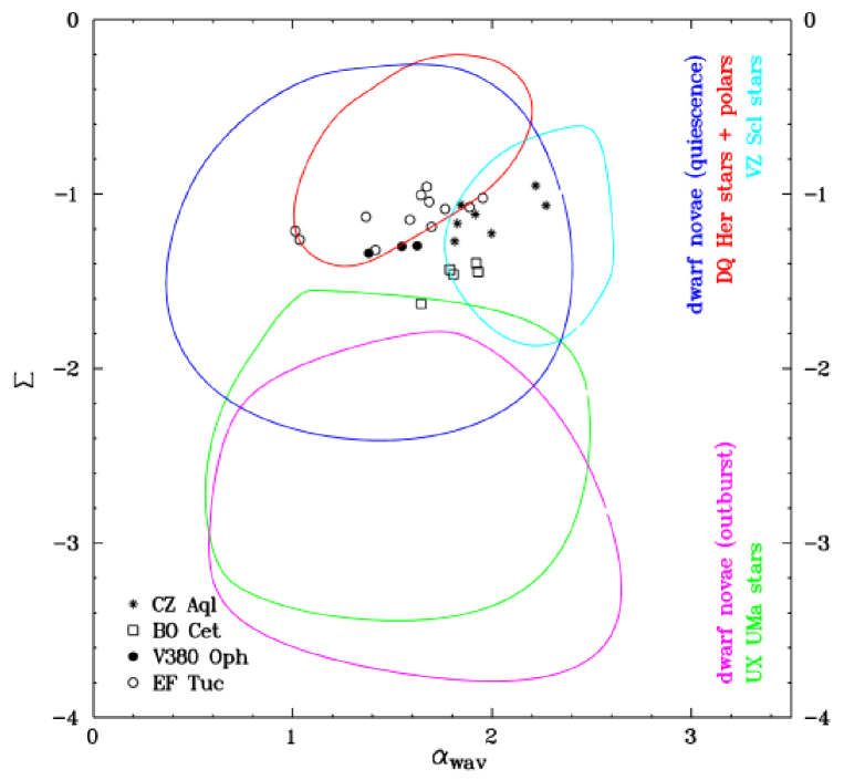
Figure 12: Scalegram parameters $\alpha_{\rm wav}$ vs. $\Sigma$ derived from a wavelet analysis of the light curves of the objects of this study. The coloured contours indicate the limits in the $\alpha_{\rm wav}-\Sigma$ plane of the range populated by CVs of different kinds and photometric states as found by Fritz & Bruch (1998).

All objects lie comfortably in the (wide) range occupied by quiescent dwarf novae. However, this does not permit a unique classification and a closer inspection is in order.

Not much is known about the long term brightness variations of CZ Aql. The AAVSO data base contains only a few data points scattered within a magnitude range compatible with the observed flickering. No outbursts were ever reported. Based on spectroscopic evidence, Sheets et al. (2007) suspected a magnetically channeled accretion flow. In Fig. 12 CZ Aql lies just outside the range of DQ Her stars (intermediate polars) and polars. It is, however, within the range of VZ Scl novalike variables. Long term monitoring in order to detect either outbursts or low states should permit to better determine the subtype of CZ Aql.

With a single outlying light curve, BO Cet lies in the range of VZ Scl novalike variables. At first sight this appears to be slightly at odds with its classification as SW Sex star (Rodríguez-Gil et al. 2007), all such systems included in the study of Fritz & Bruch (1998) having significantly smaller values of $\Sigma$. However, as Rodríguez-Gil et al. (2007) pointed out, half of the known VY Scl systems are also SW Sex stars, but none of the SW Sex stars in the sample of Fritz & Bruch (1998) is known to exhibit low states. Again, the AAVSO data base is insufficient to draw any conclusion, while a light curve generated from AEOEV data exhibits variability between $\sim$13${}^{\raisebox{0.90417pt}{\scriptsize m}}_{\raisebox{1.80835pt}{\hskip 1.18999pt.}}$7 and $\sim$15${}^{\raisebox{0.90417pt}{\scriptsize m}}_{\raisebox{1.80835pt}{\hskip 1.18999pt.}}$2 but is not dense enough to permit the identification of outbursts or low states.

The long term photometric as well as the spectroscopic evidence cited in Sect. 5 clearly identify V380 Oph as both, a SW UMa and VZ Scl type star. In the $\alpha_{\rm wav}-\Sigma$ plane it lies somewhat beyond the VZ Scl borders, which might just mean that the sample of Fritz & Bruch (1998) is too limited to encompass the entire range.

Finally, as shown in Sect. 6, EF Tuc is a genuine dwarf nova and this is corrobrated by its position in the $\alpha_{\rm wav}-\Sigma$ plane.

8.4 The intermediate and high frequency regime

Looking for consistent variations on time scales as expected to be caused, e.g., by the rotation of the white dwarf in intermediate polars or by Quasi Periodic Oscillations (QPOs) it may be misleading to turn to the power spectrum of an entire light curve. Random flickering flares, eventually accidentally recurring a few times quasi-periodically within a limited time interval, can easily cause strong power spectrum peaks which may be mistaken as indications for persistent oscillations. It is therefore more appropriate to regard time resolved power spectra.

To this end, stacked power spectra was calculated as outlined by Bruch (2014): Using the high pass filtered light curves introduced in Sect. 8.1, sections of $\Delta\tau=30\mbox{${}^{\raisebox{0.90417pt}{\scriptsize m}}$}$ duration and an overlap of 27${}^{\raisebox{0.90417pt}{\scriptsize m}}$ between successive sections were taken. For each of them a Lomb-Scargle periodogram was calculated and the individual power spectra were stacked on top of each other to result in a two-dimensional representation (frequency vs. time). An example is shown in Fig. 13 which refers to the light curve of CZ Aql of 2014, June 17. Relative power is shown on a logarithmic colour scale. To the left of the stacked power spectrum the high pass filtered light curve is shown, and above it the Lomb-Scargle periodogram of the entire data set is plotted. Due to the chosen values for $\Delta\tau$ structures on time scales of less than 30${}^{\raisebox{0.90417pt}{\scriptsize m}}$ (indicated by the double-headed arrow at the upper left of the time axis) are not independent. The false alarm probability of 0.001 for power spectrum peaks is marked on the colour bar in the upper left frame of the figure. It was calculated using Eq. 18 of Scargle (1982), the number of independent frequencies having been determined as described by Bruch & Diaz (2917). Thus, the yellow and red structures are highly significant.

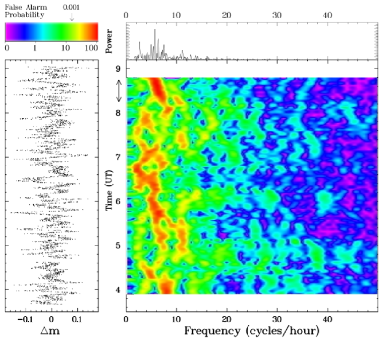
Figure 13: Light curve of CZ Aql of 2014, June 17 after removal of variations on time scales above 30${}^{\raisebox{0.90417pt}{\scriptsize m}}$ (left frame) and stacked power spectra (relative power on a logarithmic scale) of the same data (right). Spectral features within a range of 30${}^{\raisebox{0.90417pt}{\scriptsize m}}$ are not independent from each other. The length of this range is indicated by a double arrow at the upper left margin of the stacked power spectra. The upper right frame contains the power spectrum calculated from the entire data set. At the upper left, a color bar is shown, where the false alarm probability level of 0.001 is marked.

In none of the stacked power spectra features were observed which might confidently be interpreted as QPOs. However, while not conclusive, the results for CZ Aql may point at an intermediate polar nature as implied by the suspicion of Sheets et al. (2007) of a magnetically channeled accretion flow in this system. In all of the stacked power spectra strong structures occur preferentially at frequencies corresponding to periods between 9${}^{\raisebox{0.90417pt}{\scriptsize m}}_{\raisebox{1.80835pt}{\hskip 1.18999pt.}}$5 and 12${}^{\raisebox{0.90417pt}{\scriptsize m}}_{\raisebox{1.80835pt}{\hskip 1.18999pt.}}$2 which often extend in time for intervals $\gg\Delta\tau$. An example can be seen in the central part of the stacked power spectrum shown in Fig. 13. A strong signal with at a similar frequency again appears at the end of the light curve. Together, they lead to the main peak in the Lomb-Scargle periodogram in the upper frame of the figure, which corresponds to a period of 10${}^{\raisebox{0.90417pt}{\scriptsize m}}_{\raisebox{1.80835pt}{\hskip 1.18999pt.}}$6. The varying strength of such features and their shifts in frequency in the stacked power spectra can be explained by the influence of random variations: Tests with artificial sinusoidal signals even with large amplitudes (up to 50% of the total flickering amplitude) added to the real data showed that their reflection in the stacked spectra can easily be suppressed or frequency shifted during some time interval by the influence of flickering.

In Fig. 14 the high pass filtered light curve of CZ Aql of 2014, June 17, folded on the suggested period of 10${}^{\raisebox{0.90417pt}{\scriptsize m}}_{\raisebox{1.80835pt}{\hskip 1.18999pt.}}$6 and binned into phase intervals of 0.05, is shown together with the best fit sine curve. Interpreting the variations as due to the rotation of the white dwarf, the spin to orbital period ratio is thus $P_{\rm spin}/P_{\rm orb}\approx 0.037$ which is totally in line with ratio observed for the majority of intermediate polars (see, e.g., Koji Mukai’s Intermediate Polar Homepage). The total amplitude of 0${}^{\raisebox{0.90417pt}{\scriptsize m}}_{\raisebox{1.80835pt}{\hskip 1.18999pt.}}$04 is also not unusual for IPs with similar spin period (MU Cam, Staude et al. 2003; PQ Gem, Evans et al. 2006; NY Lup, Haberl et al. 2002).

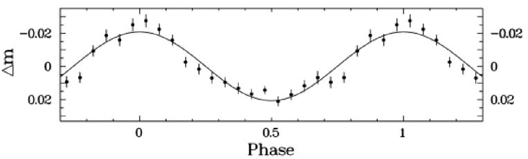
Figure 14: Light curve of CZ Aql of 2014, June 17 (dots) after removal of variations on time scales above 30${}^{\raisebox{0.90417pt}{\scriptsize m}}$, folded on period 10${}^{\raisebox{0.90417pt}{\scriptsize m}}_{\raisebox{1.80835pt}{\hskip 1.18999pt.}}$6 and binned in intervals of width 0.05 in phase. The error bars represent mean errors of the mean. The solid line is a least squares sine fit the the data.

While by far not sufficient to classify CZ Aql as an intermediate polar, the evidence presented here, together with the proximity of the object to the intermediate polars in the $\alpha_{\rm wav}-\Sigma$ plane (see Sect. 8.3), the spectroscopic indications quoted by Sheets et al. (2007) and the presence of a rather strong He II $\lambda$ 4686 Å  emission line seen in the spectrum of Cieslinski et al. (1998) – a feature not exclusive to but typical for magnetic CVs – justifies to further consider this hypothesis. To prove or disprove it will require additional observations.

9 Summary

I have presented the first time resolved photometry for an ensemble of five cataclysmic variables and candidates. While four of them (CZ Aql, BO Cet, V380 Oph and EF Tuc) are established members of the class, based on previous spectroscopic studies, Lib 3 was only suspected to be a CV. The absence of flickering – a sine qua non for all CVs – in the latter star justifies to remove Lib 3 from the list of CV candidates.

All other targets of this study exhibit pronounced flickering. This is an indication that their accretion disks are not in a stable bright state as is observed in nova-like variables of the UX UMa class or most old novae, which have much smaller flickering amplitudes (Fritz & Bruch 1998). The flickering behaviour rather points at a VY Scl type classification for BO Cet and V380 Oph (in the latter case confirmed by its long-term light curve), in addition to their classification as SW Sex stars (Rodríguez-Gil et al. (2007). EF Tuc is a genuine dwarf nova, observed in quiescence, while the evidence for CZ Aql is unclear. It may be a VY Scl type star or a dwarf nova. Additionally, a nature as intermediate polar cannot be discarted.

Variations on hourly time scales reveal clear orbital modulations in BO Cet during the 2014 observing season, which, however, are not as clear in 2016. Orbital modulations were probably also observed in V380 Oph. On the other hand, a modulation with a period $\sim$8% longer than the orbital period was observed in CZ Aql which may be similar to variations interpreted as superhumps in several other (non SU UMa type) system, many of which are known VY Scl stars.

References

Allen, C.W. 1973, Astrophysical Quantities, third edition (Athlone Press: London)

Anzolin, G., Tamburini, F., de Martino, D., & Bianchini, A. 2010, A&A 519, A69

Beers, T.C., Preston, G.W., Shectman, S.A., Doinidis, S.P., & Griffin, K.E. 1992, AJ, 103, 267

Belova, A.I., Suleimanov, V.F., Bikmaev, I.F., et al. 2013, Astron. Letters, 39, 111

Bruch, A. 1991, Acta Astron, 41, 101

Bruch, A. 1992, A&A 266, 237

Bruch, A. 1993, A Reference Guide (Astron. Inst. Univ. Münster

Bruch, A. 2014, A&A, 566, A101

Bruch, A. 2016, New Astr., 46, 90

Bruch, A., Diaz, M.P. 2017, New Astr., 50, 109

Chen, A., O’Donogue, D., Stobie, R.S., Kilkenny, D., Warner, B. 2001 MNRAS, 385, 89

Cieslinski, D., Steiner, J.E., & Jablonski, F.J. 1998, A&AS 131, 119

Da Costa, G.M. 1992, ASP Conf. Ser., 23, 90

Downes, R.A., Webbink, R.F., Shara, M.M., et al. 2005, J. Astron. Data, 11, 2

Eastman, J., Siverd, R., & Gaudi, B.S. 2010, PASP, 122, 935

Evans, P.A., Hellier, C., & Ramsay, G. 2006, MNRAS, 369, 1229

Fritz, T., Bruch, A. 1998, A&A, 332, 586

Garcia, A, Sodré Jr., L., Jablonski, F.J., & Terlevich, R.J. 1999, MNRAS, 309, 803

Gromadzki, M., Mikołajewski, M., Tomov, T., et al. 2006, Acta Astron., 56, 97

Haberl, F., Motch, C., & Zickegraf, F.-J. 2002, A&A, 387, 201

Haefner, R., Metz, K. 1985, A&A, 145, 311

Herbst, W., & Shevchenko, V.S. 1999, AJ, 118, 1043

Hoffmeister, C. 1929, Mitt. Sternw. Sonneberg, N16

Horne, J.H., & Baliunas, S.L. 1986, ApJ, 302, 757

Kafka, S., & Honeycutt, R.K. 2004, Rev. Mex. A&A (Conf. Series), 20, 238

Kato, T., Imada, A., & Uemura, M. 2009, PASJ, 61, S395

Kazarovetz, E.V., Samus, N.N., & Goranskij, V.P. 1993, IBVS 3840

Kenyon, S.J., Kolotilov, E.A., Ibragimov, M.A., & Mattei, J.A. 2000, ApJ, 531, 1028

Kozhevnikov, V.P. 2007, MNRAS, 378, 955

Kozhevnikov, V.P. 2012, New Astron., 17, 38

Liu, W., Hu, J.Y., Li, Z.Y., & Cao, L. 1999a, ApJS, 122, 257

Liu, W., Hu, J.Y., Zhu, X.H., & Li, Z.Y. 1999b, ApJS, 122, 243

Lomb, N.R. 1976, Ap&SS, 39, 447

Papadaki, C., Boffin, H.M.J., Stanishev, V., et al. 2009, J. Astron. Data, 15, 1

Papadaki, C., Boffin, H.M.J., Sterken C., et al. 2006, A&A, 456, 599

Patterson, J., Thomas, G., Skillman, D.R., Diaz, M. 1993, ApJ Suppl., 86, 235

Patterson, J., Thorstensen J.R., Fried, R., et al. 2001, PASP, 113, 72

Reinmuth, K. 1925, Astron, Nachr. 225, 385

Ritter, H., Kolb, U. 2003, A&A, 404, 301

Rodríguez-Gil, P., Schmidtobreik, L., & Gänsicke, B. 2007 MNRAS, 374, 1359

Scargle, J.D. 1982, ApJ, 263, 853

Scargle, J.D., Steiman-Cameron, T.Y., Young, K., et al. 1993, ApJ 411, L91

Scaringi, S., Maccarone, T.J., Körding, E., et al. 2015, Science Adv., 1, e1500686

Schwarzenberg-Czerny, A. 1989, MNRAS 241, 153

Shafter, A.W. 1983, IBVS, 2377

Shafter, A.W. 1985, AJ, 90, 643

Sheets, H.A., Thorstensen, J.R., Peters, C.J., & Kapusta, A.B. 2007, PASP, 119, 494

Shugarov, S.Yu., Katysheva, N.A., Seregina, T.M., & Volkov,I.M. 2005, in: The Astrophysics of Cataclysmic Variables and Related Objects (eds: J.-M. Hameury & J.-P. Lasota), ASP Conf. Series, 330, p. 495

Smak, J. 2013, Acta Astron., 17, 453

Staude, A, Schwope, A.D., Krumpe, M., Hambaryan, V., & Schwarz, R. 2003, A&A, 406, 253

Stellingwerf, R.F. 1978, ApJ, 224, 953

Stobie, R.S., Kilkenny, D., O’Donoghue, D. 1995, ApSS, 230, 101

Tamburini, F., de Martino, D., & Bianchini, A. 2010, A&A 502, 1

van der Klis, M. 2004, arXiv e-prints [arXiv:astro-ph/0410551]

Verbunt, F., Bunk, W.H., Ritter, H., & Pfeffermann, E. 1997, A&A 327, 602

Vogt, N. 1989, in: Classical Novae, ed. M.F. Bode and A. Evans (New York, Wiley and Sons), p. 225

Zacharias, N., Finch, C.T., Girard, T.M., et al. 2013, AJ, 145, 44

Zwitter, T., & Munari, U. 1995, A&AS, 114, 575