Foldy-Wouthuysen transfer matrix method for Dirac tunneling through monolayer graphene with a mass gap

Abstract

I provide a transfer matrix method for the Foldy-Wouthuysen representation of the Dirac equation. I develop the relationship between the reflection and transmission coefficients of the Dirac spinors and the wavefunction in the transformed representation. I develop a WKB approximation for Dirac fermions which has the same elegant form as the WKB solution to Schrödinger’s equation. My WKB approximation is to all orders and includes the semi-classical turning point. I provide an extension to fully $2$-dimensional periodic structures by Fourier methods for band engineering. I verify my methods for all energies by comparison with analytic solutions developed in the Dirac spinor representation. I also include a rich appendix detailing my research into the Green’s functions of Dirac fermions.

1 Introduction

In Refs. [1, 2, 3] the pseudo-relativistic dispersion of $2$-dimensional ($2$D) materials was investigated theoretically for the emergence of extra Dirac points with $1$D periodic barriers. The method employed was the application of Bloch’s theorem to transfer matrices of Dirac spinors. These band engineering studies attracted considerable interest since the vanishing band gap of $2$D materials is an Achilles heel for applications. Other methods for band engineering that open the way to creating $2$D semiconductor materials include strain engineering [4], vertical stacking [5], and chemical doping [6].

Armed with the knowledge to create semiconductor $2$D materials a theoretical study of the operational window for negative differential resistance was pursued by other authors [7]. The mathematical method employed in their study was the application of transfer matrices to the Dirac spinors of a rotated Dirac Hamiltonian derived in Ref. [8].

Motivated by the study of unconventional transmission and density of states, the modeling of Dirac fermions has moved beyond unrealistic square barrier systems. In experimental devices barriers are more often smoothly varying, semi-classical (WKB) methods are needed. An approach using separate Hamiltonians for electrons and holes in Ref. [9] gave way in Ref. [10] to an expansion in powers of $\hbar$ partly resembling the WKB method for the Schrödinger equation. However it is acknowledged by the authors of Refs. [9, 10] that their mathematical approaches to semi-classical analysis can be divergent at the classical turning point.

The contribution to the theory of tunneling in $2$D materials that I present in this article is the application of the Foldy-Wouthuysen (FW) representation of the Dirac equation.

Whilst the FW transformation was first conceived as a semi-relativistic representation of the Dirac equation [11], I will show, through my rigorous derivations in Section 2 to Section 13 and my analytic and numerical verification of Section 14 and Appendix B, that the FW representation remains an exactly accurate representation of the Dirac equation for all energies.

I find that the FW representation allows a derivation of the relativistic WKB approximation, Section 7 to Section 10, in the same elegant form as the approximate WKB solution to Schrödinger’s equation. Since at low energies the FW representation reduces to the Schrödinger equation, I have found, in Section 11, a simple method to mathematically describe the connections between WKB regions.

Fourier analysis is used in Section 12 to apply my approach to fully $2$D periodic structures. Section 12 offers the prospect of extending the scope of the band engineering studies made in Refs. [1, 2, 3]. My numerical and analytic results showing that the FW equation is an exactly accurate representation of relativistic fermions, for all energies, will be important here. The Fourier transform method in Section 12 requires expansion of the wavefunction in plane waves of momentum beyond semi-relativistic energies.

In Appendix E I make the reader aware of a limit to appealing for solutions of the Dirac equation from its FW representation, I reveal and discuss a Green’s function (GF) paradox arising when transforming between the two representations.

My article is organized as follows: Section 2 outlines the derivation of the FW representation from the Dirac equation. Section 3 gives the transmission of the Dirac equation in terms of the transmission of its FW representation. Section 4 derives the boundary conditions of the FW equation at sharp steps in potential. Section 5 and Section 6 develop the transfer matrices for square barriers and delta potentials. Section 7, Section 8, Section 9 and Section 10 give a $1st$, iterative and $2nd$ order WKB approximations for two interpretations of the FW equation. Section 11 gives the connecting formulae between regions where the WKB approximation is appropriate. Section 12 extends my approach to include periodic structures. Section 13 details how I evaluated the boundary conditions. Section 14 gives numerical results for examples of tunneling through barriers and resonant diodes.

The appendices are organized as follows: Appendix A analytically justifies my commutation of FW wavefunction operators. Appendix B analytically calculates the reflection at a step in both the Dirac spinor and FW representations for comparison. Appendix C examines the tunneling of a massless fermion through a magnetic delta barrier in the FW representation. Appendix D calculates GFs of the FW equation. Appendix E uncovers a relativistic GF paradox.

2 Dirac equation and its Foldy-Wouthuysen representation

The Dirac equation for a scalar potential $V$ is given in Hamiltonian form by

$$\left[c{\bf\alpha}\cdot\hat{p}+\beta mc^{2}\right]\Psi=H\Psi=\left(E+V\right)\Psi\,,$$ (1)

$$\gamma_{t}=\begin{pmatrix}{+I}&0\\ 0&{-I}\end{pmatrix}\,,\qquad\gamma_{x,y,z}=\begin{pmatrix}0&{+\sigma_{x,y,z}}\\ {-\sigma_{x,y,z}}&0\end{pmatrix}\,,$$ (2)

$$I=\begin{pmatrix}{+1}&0\\ 0&{+1}\end{pmatrix}\,,\qquad\sigma_{x}=\begin{pmatrix}0&{+1}\\ {+1}&0\end{pmatrix}\,,$$ (3)

$$\sigma_{y}=\begin{pmatrix}0&{-i}\\ {+i}&0\end{pmatrix}\,,\qquad\sigma_{z}=\begin{pmatrix}{+1}&0\\ 0&{-1}\end{pmatrix}\,,$$ (4)

with ${\alpha_{x,y,z}}=\gamma_{t}\gamma_{x,y,z}$ and $\beta=\gamma_{t}$.

$$\hat{p}=-i\hbar{\bf\nabla}=-i\hbar\left[\dfrac{\partial}{\partial x},\dfrac{\partial}{\partial y},\dfrac{\partial}{\partial z}\right]$$ (5)

is the momentum operator for the electron which is of mass $m$ and energy $E$. The charge and current density are given by the following well known expressions:

$$\rho=\Psi^{*}\Psi\,,$$ (6)

$$j=\Psi^{*}\alpha\Psi\,.$$ (7)

There are two linearly independent solutions of the free particle Dirac equation,

$$\Psi^{\left(\pm\right)}_{\uparrow}=\begin{pmatrix}\mp mc^{2}-E-V\\ 0\\ 0\\ c\left(p_{x}\pm ip_{y}\right)\end{pmatrix}\exp{\left(\dfrac{ip_{x}x+ip_{y}y}{\hbar}\right)}\,,$$ (8)

$$\Psi^{\left(\pm\right)}_{\downarrow}=\begin{pmatrix}0\\ \mp mc^{2}-E-V\\ c\left(p_{x}\mp ip_{y}\right)\\ 0\end{pmatrix}\exp{\left(\dfrac{ip_{x}x+ip_{y}y}{\hbar}\right)}\,,$$ (9)

each can be normalised to one electron per unit volume by Eq. (6).

By making use of the FW transformation I will decouple the differential equations of the Dirac equation to give four independent identical equations. I will show that by calculating the propagation for only one of these components I may obtain the full GF and transmission.

Under unitary transformation the Dirac equation becomes

$$e^{+iS}He^{-iS}e^{+iS}\Psi=\left(E+V\right)e^{+iS}\Psi\,.$$ (10)

Foldy and Wouthuysen [11] found that their rotation

$$e^{\pm iS}=\cos\theta\pm{\bf\beta}{\bf\alpha}\cdot\dfrac{\hat{p}}{\left|\hat{p}\right|}\sin\theta\,,$$ (11)

transformed the Dirac Hamiltonian into diagonal and anti-diagonal parts

$$\beta\left(mc^{2}\cos{\left(2\theta\right)}+c\left|\hat{p}\right|\sin{\left(2\theta\right)}\right)\\ +c\alpha\cdot\hat{p}\left(\cos{\left(2\theta\right)}-\dfrac{mc}{\left|\hat{p}\right|}\sin{\left(2\theta\right)}\right)\\ =e^{+iS}He^{-iS}\,.$$ (12)

Subsequently it was chosen [11]

$$\cos\left(2\theta\right)=\dfrac{mc^{2}}{\sqrt{c^{2}\hat{p}^{2}+m^{2}c^{4}}}\,,$$ (13)

$$\sin\left(2\theta\right)=\dfrac{c\left|\hat{p}\right|}{\sqrt{c^{2}\hat{p}^{2}+m^{2}c^{4}}}\,,$$ (14)

so that by direct substitution of Eq. (13) and Eq. (14) into Eq. (12)

$$\left[{\bf\beta}\sqrt{\hat{p}^{2}c^{2}+m^{2}c^{4}}-\hat{1}\left(V+E\right)\right]\widetilde{\Psi}=0\,.$$ (15)

Eq. (15) shows there are two possibilities for the FW equation

$$\left[\mp\sqrt{\hat{p}^{2}c^{2}+m^{2}c^{4}}-\left(V+E\right)\right]\widetilde{\Psi}^{\left(\pm\right)}=0\,,$$ (16)

$\widetilde{\Psi}^{\left(-\right)}$ corresponds to the electron, $\widetilde{\Psi}^{\left(+\right)}$ to the positron. The rotated wavefunction $\widetilde{\Psi}$ is related to $\Psi$ by

$$\left[\cos\theta+{\bf\beta}{\bf\alpha}\cdot\dfrac{\hat{p}}{\left|\hat{p}\right|}\sin\theta\right]\Psi=\widetilde{\Psi}\,.$$ (17)

Taylor expanding $\sqrt{\hat{p}^{2}c^{2}+m^{2}c^{4}}$ in Eq. (16) gives

$$\left[\mp\mathcal{L}-\left(V+E\pm mc^{2}\right)\right]\widetilde{\Psi}^{\left(\pm\right)}=0\,,$$ (18)

where

$$\mathcal{L}=mc^{2}\left[\dfrac{1}{2}\left[{\dfrac{\hat{p}}{mc}}\right]^{2}-\dfrac{1}{8}\left[{\dfrac{\hat{p}}{mc}}\right]^{4}+\dfrac{1}{16}\left[{\dfrac{\hat{p}}{mc}}\right]^{6}-...\right]\,.$$ (19)

Eq. (16) and Eq. (18) are two interpretations of the FW equation.

I demonstrate the unsuitability of my FW approach for calculating magnetic barrier tunneling in Appendix C. I discuss the GFs of the FW Eq. (18) in Appendix D. I uncover and discuss a GF paradox of the FW Eq. (18) in Appendix E.

3 Relationship between the transmission of the Dirac equation and its Foldy-Wouthuysen representation

Throughout my numerical and analytic results, Section 14 and Appendix B, I will calculate the reflection coefficient $R$ to deduce the transmission coefficient $T$ as

$$T=1-R\,.$$ (20)

Calculating $R$, rather than $T$ directly, does not require the normalisation of the wavefunction in both the incident and transmitted regions.

Let $\Psi$ be given by Eq. (8) and Eq. (9) as

$$\Psi=u\exp{\left(\dfrac{ip_{x}x+ip_{y}y}{\hbar}\right)}\,,$$ (21)

taking $\widetilde{\Psi}$ of the form

$$\widetilde{\Psi}=\widetilde{u}\exp{\left(\dfrac{ip_{x}x+ip_{y}y}{\hbar}\right)}\,,$$ (22)

I find by application of Eq. (17) to Eq. (21)

$$\begin{split}&\widetilde{u}_{1}=u_{1}\cos\theta+\left(d_{x}-id_{y}\right)u_{4}\sin\theta\,,\\ &\widetilde{u}_{2}=u_{2}\cos\theta+\left(d_{x}+id_{y}\right)u_{3}\sin\theta\,,\\ &\widetilde{u}_{3}=u_{3}\cos\theta-\left(d_{x}-id_{y}\right)u_{2}\sin\theta\,,\\ &\widetilde{u}_{4}=u_{4}\cos\theta-\left(d_{x}+id_{y}\right)u_{1}\sin\theta\,,\end{split}$$ (23)

where $\hat{d}=\hat{p}/|\hat{p}|$.

Eq. (21), Eq. (22), and Eq. (LABEL:FWtoDirac1) show $\widetilde{\Psi}$ in exponential planar form which is useful for calculating the fermion propagation through homogeneous space.

The incident ($i$) and reflected ($r$) waves for planar structures in the Dirac equation description are related to the reflection coefficient in the well known way:

$$R=\dfrac{\left(\Psi\cdot\Psi^{*}\right)^{\left(r\right)}}{\left(\Psi\cdot\Psi^{*}\right)^{\left(i\right)}}\,.$$ (24)

For the two linearly independent solutions of the Dirac equation, Eq. (8) and Eq. (9), Eq. (24) gives rise to two degenerate expressions for the reflection coefficient:

$$R_{\uparrow}=\dfrac{\left(\left|\Psi_{1}\right|^{2}+\left|\Psi_{4}\right|^{2}\right)^{(r)}}{\left(\left|\Psi_{1}\right|^{2}+\left|\Psi_{4}\right|^{2}\right)^{\left(i\right)}}\,,$$ (25)

$$R_{\downarrow}=\dfrac{\left(\left|\Psi_{2}\right|^{2}+\left|\Psi_{3}\right|^{2}\right)^{\left(r\right)}}{\left(\left|\Psi_{2}\right|^{2}+\left|\Psi_{3}\right|^{2}\right)^{\left(i\right)}}\,.$$ (26)

I take note of Eqs. (LABEL:FWtoDirac1) linking $\widetilde{u}$ to $u$ and calculate when $d$ is real

$$\left|\widetilde{u}_{1}\right|^{2}+\left|\widetilde{u}_{4}\right|^{2}=\left|u_{1}\right|^{2}+\left|u_{4}\right|^{2}\,,$$ (27)

$$\left|\widetilde{u}_{2}\right|^{2}+\left|\widetilde{u}_{3}\right|^{2}=\left|u_{2}\right|^{2}+\left|u_{3}\right|^{2}\,,$$ (28)

therefore $R$ described by the Dirac equation can be rewritten in terms of the FW wavefunctions:

$$R_{\uparrow}=\dfrac{\left(\left|\widetilde{\Psi}_{1}\right|^{2}+\left|\widetilde{\Psi}_{4}\right|^{2}\right)^{\left(r\right)}}{\left(\left|\widetilde{\Psi}_{1}\right|^{2}+\left|\widetilde{\Psi}_{4}\right|^{2}\right)^{\left(i\right)}}\,,$$ (29)

$$R_{\downarrow}=\dfrac{\left(\left|\widetilde{\Psi}_{2}\right|^{2}+\left|\widetilde{\Psi}_{3}\right|^{2}\right)^{\left(r\right)}}{\left(\left|\widetilde{\Psi}_{2}\right|^{2}+\left|\widetilde{\Psi}_{3}\right|^{2}\right)^{\left(i\right)}}\,.$$ (30)

Since the components of $\widetilde{\Psi}$ are degenerate I am only required to evaluate the propagation of a fermion by the FW Eq. (18) once when calculating $R$ and $T$.

4 Boundary Conditions of the Foldy-Wouthuysen equation at a sharp step

Consider a sharp step in potential at $x=a$. I will integrate the FW Eq. (18) through the boundary, normal to the boundary

$$\lim_{\left({a_{+}}-{a_{-}}\right)\rightarrow 0}\int^{a_{+}}_{a_{-}}\left[\mp\mathcal{L}-\left(V+E\pm mc^{2}\right)\right]\widetilde{\Psi}^{\left(\pm\right)}\dfrac{dx}{c\hbar}=0\,.$$ (31)

In this section I introduce the operator $\mathcal{\accentset{\rule{2.79996pt}{0.7pt}}{L}}$ which commutes with $c\hat{p}_{x}$ and is defined by

$$\mathcal{L}\widetilde{\Psi}=-\mathcal{\accentset{\rule{2.79996pt}{0.7pt}}{L}}c\hat{p}_{x}\widetilde{\Psi}=-c\hat{p}_{x}\mathcal{\accentset{\rule{2.79996pt}{0.7pt}}{L}}\widetilde{\Psi}\,.$$ (32)

I give a discussion of Eq. (32) in Appendix A.

Since

$$\lim_{\left({a_{+}}-{a_{-}}\right)\rightarrow 0}\int^{a_{+}}_{a_{-}}\left(V+E\pm mc^{2}\right)\widetilde{\Psi}^{\left(\pm\right)}\dfrac{dx}{c\hbar}=0\,,$$ (33)

due to the function integrated being finite but the integration range tending to zero, I have

$$\left[i\mathcal{\accentset{\rule{2.79996pt}{0.7pt}}{L}}\widetilde{\Psi}\right]^{a_{+}}_{a_{-}}=\lim_{\left({a_{+}}-{a_{-}}\right)\rightarrow 0}\int^{a_{+}}_{a_{-}}\mathcal{L}\widetilde{\Psi}\dfrac{dx}{c\hbar}=0\,.$$ (34)

I can understand Eq. (34) when I consider that

$$\mathcal{L}\widetilde{\Psi}=ic\hbar\dfrac{\partial\left(\mathcal{\accentset{\rule{2.79996pt}{0.7pt}}{L}}\widetilde{\Psi}\right)}{\partial x}\,.$$ (35)

Eq. (34) shows that $\widetilde{\Psi}$ is continuous with respect to the operation of $\mathcal{\accentset{\rule{2.79996pt}{0.7pt}}{L}}$.

In order to evaluate $\mathcal{\accentset{\rule{2.79996pt}{0.7pt}}{L}}\widetilde{\Psi}$ for the mathematical description of the boundary conditions note

$$\pm\mathcal{\accentset{\rule{2.79996pt}{0.7pt}}{L}}c\hat{p}_{x}\widetilde{\Psi}^{\left(\pm\right)}=\left(V+E\pm mc^{2}\right)\widetilde{\Psi}^{\left(\pm\right)}=\pm cp_{x}\mathcal{\accentset{\rule{2.79996pt}{0.7pt}}{L}}\widetilde{\Psi}^{\left(\pm\right)}\,,$$ (36)

therefore

$$\mathcal{\accentset{\rule{2.79996pt}{0.7pt}}{L}}\widetilde{\Psi}^{\left(\pm\right)}=\pm\dfrac{V+E\pm mc^{2}}{cp_{x}}\widetilde{\Psi}^{\left(\pm\right)}=\mp\alpha^{\left(\pm\right)}\widetilde{\Psi}^{\left(\pm\right)}\,.$$ (37)

For my second boundary condition I note that $\hat{p}\widetilde{\Psi}$ always gives a finite observed value, therefore $\widetilde{\Psi}$ is continuous everywhere.

My boundary conditions are in stark contrast to the continuity conditions of the Klein-Gordon equation, in that case continuity is with respect to momentum and wavefunction. I verify my boundary conditions numerically and analytically in Section 14 and Appendix B.

5 Transfer matrices for a square potential barrier

Inside a layer thickness $D$ the transfer matrix of $\widetilde{\Psi}$ is given by

$$\begin{pmatrix}{\exp{\left(-\dfrac{iDp_{x}}{\hbar}\right)}}&0\\ 0&{\exp{\left(+\dfrac{iDp_{x}}{\hbar}\right)}}\end{pmatrix}\begin{pmatrix}\widetilde{a}_{1}\\ \widetilde{b}_{1}\end{pmatrix}=\begin{pmatrix}\widetilde{a}_{0}\\ \widetilde{b}_{0}\end{pmatrix}\,,$$ (38)

where $\widetilde{a}_{0}$ and $\widetilde{a}_{1}$ denote forward traveling FW wave parts and $\widetilde{b}_{0}$ and $\widetilde{b}_{1}$ denote backward travelling FW wave parts, $0$ denotes on the left, $1$ denotes on the right. The fermion is refracted at the angle $\phi$ to the layer boundary normal, where

$$p_{x}=p\cos\phi\,.$$ (39)

For a boundary at a sharp step, applying the wavefunction continuity condition set out in Section 4 gives

$$\widetilde{a}_{0}+\widetilde{b}_{0}=\widetilde{a}_{1}+\widetilde{b}_{1}\,.$$ (40)

Secondly, applying wavefunction continuity under the operation of $\mathcal{\accentset{\rule{2.79996pt}{0.7pt}}{L}}$, derived in Section 4, to Eq. (40) gives

$$\alpha_{0}\widetilde{a}_{0}-\alpha_{0}\widetilde{b}_{0}=\alpha_{1}\widetilde{a}_{1}-\alpha_{1}\widetilde{b}_{1}\,.$$ (41)

Eq. (40) and Eq. (41) can be written in matrix form as

$$\dfrac{1}{2}\begin{pmatrix}{\left(1+\dfrac{\alpha_{1}}{\alpha_{0}}\right)}&{\left(1-\dfrac{\alpha_{1}}{\alpha_{0}}\right)}\\ {\left(1-\dfrac{\alpha_{1}}{\alpha_{0}}\right)}&{\left(1+\dfrac{\alpha_{1}}{\alpha_{0}}\right)}\end{pmatrix}\begin{pmatrix}\widetilde{a}_{1}\\ \widetilde{b}_{1}\end{pmatrix}=\begin{pmatrix}\widetilde{a}_{0}\\ \widetilde{b}_{0}\end{pmatrix}\,.$$ (42)

In the event of tunneling, wave modes become an exponentially decaying and growing set. Transfer matrix multiplication combines these large and small values, this process is numerically unstable and inaccurate. Instead I suggest using the method of Refs. [12, 13] to combine my transfer matrices. The method of Refs. [12, 13] addresses these instability issues by separating the exponentially growing and decaying terms.

6 Transfer matrix for a delta potential barrier

Integrating Eq. (18), with $V(x)=g\delta(x)$ and with respect to $dx/c\hbar$, across $\left[0_{-},0_{+}\right]$ gives

$$\left[\mp i\mathcal{\accentset{\rule{2.79996pt}{0.7pt}}{L}}\left(\widetilde{a}^{\left(\pm\right)}+\widetilde{b}^{\left(\pm\right)}\right)\right]^{0_{+}}_{0_{-}}=\dfrac{g}{c\hbar}\left(\widetilde{a}^{\left(\pm\right)}+\widetilde{b}^{\left(\pm\right)}\right)\biggr{\rvert}_{x=0}\,.$$ (43)

Continuity of the wavefunction gives

$$\widetilde{a}_{0}+\widetilde{b}_{0}=\widetilde{a}_{1}+\widetilde{b}_{1}\,.$$ (44)

Eq. (43) and Eq. (44) can be written in the following matrix form

$$\begin{pmatrix}{\left(1-\dfrac{ig}{2c\hbar\alpha_{k}}\right)}&{\left(-\dfrac{ig}{2c\hbar\alpha_{k}}\right)}\\ {\left(+\dfrac{ig}{2c\hbar\alpha_{k}}\right)}&{\left(1+\dfrac{ig}{2c\hbar\alpha_{k}}\right)}\end{pmatrix}\begin{pmatrix}\widetilde{a}_{1}\\ \widetilde{b}_{1}\end{pmatrix}=\begin{pmatrix}\widetilde{a}_{0}\\ \widetilde{b}_{0}\end{pmatrix}\,,$$ (45)

where I define $\widetilde{a}_{0}$, $\widetilde{a}_{1}$, $\widetilde{b}_{0}$, and $\widetilde{b}_{1}$ in the same way as Section 5.

7 ${\bf 1st}$ order relativistic WKB approximation

Consider the following result from Appendix D derived from the correct fermion interpretation of the FW equation in terms of $\mathcal{L}$,

$$T\left(k\right)=\dfrac{\left(2\alpha_{k}\alpha_{q}\right)^{2}}{\left(\alpha^{2}_{q}-\alpha^{2}_{k}\right)^{2}\sin^{2}\left(\dfrac{2m^{*}qa}{\hbar}\right)+\left(2\alpha_{k}\alpha_{q}\right)^{2}}$$ (46)

for a rectangular barrier given by

$$V\left(x\right)=\left\{\begin{array}[]{lc}V&\mbox{for}\ \ \left|x\right|<a\,,\\ 0&\mbox{for}\ \ \left|x\right|>a\,.\end{array}\right.$$ (47)

Eq. (46) can be approximated as

$$T\left(k\right)\approx\left(\dfrac{2\alpha_{k}\alpha_{q}}{\alpha^{2}_{k}-\alpha^{2}_{q}}\right)^{2}\exp{\left(-\dfrac{4im^{*}qa}{\hbar}\right)}$$ (48)

by assuming exponential wavefunction decay within the barrier. Taking logarithms of Eq. (48), the non-logarithmic term dominates the logarithmic term so that

$$\log_{e}T\left(k\right)\approx-\dfrac{4im^{*}qa}{\hbar}\,.$$ (49)

Assuming independence of transmission events, the total transmission probability for crossing an overall barrier is

$$T\approx\prod_{i=1}^{\infty}T_{i}\,,$$ (50)

$$\log_{e}\prod_{i=1}^{\infty}T_{i}\approx\sum_{i=1}^{\infty}-\dfrac{2im^{*}_{i}q_{i}\Delta x}{\hbar}=-\dfrac{2i}{\hbar}\int p_{x}dx\,,$$ (51)

where the $T_{i}$ are the transmission probabilities of the individual barriers. I see from Eq. (51) that inside a smoothly varying layer the FW wavefunction is approximately given by

$$\widetilde{\Psi}\approx\exp{\left({\pm\dfrac{i}{\hbar}\int p_{x}dx}\right)}\prod_{i=1}^{N}\left(\dfrac{2\alpha_{k}\alpha_{q}}{\alpha^{2}_{k}-\alpha^{2}_{q}}\right)_{i}\,.$$ (52)

8 Iterative relativistic WKB approximation

Consider a wavefunction of the form

$$\widetilde{\Psi}=\exp{\left(\dfrac{i\Phi}{\hbar}\right)}\,,$$ (53)

then the boson FW interpretation Eq. (16) becomes

$$\left[\sqrt{c^{2}\left(\dfrac{\partial\Phi}{\partial x}\right)^{2}-c^{2}i\hbar\dfrac{\partial^{2}\Phi}{\partial x^{2}}+m^{2}c^{4}}-\left(V+E\right)\right]\widetilde{\Psi}=0\,.$$ (54)

Eq. (54) can be exactly rewritten as

$$c^{2}\left(\dfrac{\partial\Phi}{\partial x}\right)^{2}-c^{2}i\hbar\dfrac{\partial^{2}\Phi}{\partial x^{2}}+m^{2}c^{4}=\left(V+E\right)^{2}\,.$$ (55)

I now make use of $(E+V)^{2}=m^{2}c^{4}+p^{2}c^{2}$ in Eq. (55) and find that as expected

$$\hat{p}^{2}_{x}\widetilde{\Psi}=p^{2}_{x}\widetilde{\Psi}\,,\qquad\dfrac{\partial\Phi}{\partial x}=\sqrt{p^{2}_{x}+i\hbar\dfrac{\partial^{2}\Phi}{\partial x^{2}}}\,.$$ (56)

I know from Section 7

$$\pm\dfrac{\partial\Phi}{\partial x}\approx p_{x}\,,$$ (57)

suggesting a next approximation on from Eq. (52) is

$$\Phi\approx\pm\int\sqrt{p^{2}_{x}\pm i\hbar\dfrac{\partial p_{x}}{\partial x}}dx\,.$$ (58)

Eq. (58) follows from the integration of Eq. (56). This procedure can be iterated to an $n^{th}$ order WKB approximation in the boson FW interpretation.

9 ${\bf 2nd}$ order relativistic WKB approximation

Expanding $\Phi\left(x\right)$ in powers of $\hbar$

$$\Phi\left(x\right)=\Phi_{0}\left(x\right)+\hbar\Phi_{1}\left(x\right)+\hbar^{2}\Phi_{2}\left(x\right)+...\,,$$ (59)

then substituting Eq. (59) into Eq. (56) gives

$$\left(\Phi_{0}^{\prime}+\hbar\Phi_{1}^{\prime}+...\right)^{2}-i\hbar\left(\Phi_{0}^{\prime\prime}+\hbar\Phi_{1}^{\prime\prime}+...\right)=p^{2}_{x}\,.$$ (60)

Equating terms in powers of $\hbar$, in Eq. (60), I see

$$\pm\Phi_{0}^{\prime}=p_{x}\,,\qquad 2\Phi_{0}^{\prime}\Phi_{1}^{\prime}-i\Phi_{0}^{\prime\prime}=0\,,$$ (61)

so that

$$\Phi_{0}=\pm\int p_{x}dx\,,\qquad\Phi_{1}=\dfrac{i}{2}\log_{e}\Phi_{0}^{\prime}\,.$$ (62)

Eqs. (62), Eq. (59), and Eq. (53) give

$$\widetilde{\Psi}\approx\dfrac{\exp{\left(\pm\dfrac{i}{\hbar}\int p_{x}dx\right)}}{\sqrt{p_{x}}}\,.$$ (63)

This result is identical to the Klein-Gordon WKB approximation because on the way I approximated FW Eq. (18) with Eq. (16).

10 Discussion of fermion and boson WKB approximations

When I made my WKB approximation in Section 7, from what I will show in Section 14 and Appendix B to be the correct form Eq. (18) of the FW equation, I saw in the non-exponential factor of Eq. (48) appearances of $p_{i}$ changed to appearances of $\alpha_{i}$ going from boson to fermion descriptions. I have noticed, that for tunneling through slowly varying potentials, Eq. (48), Eq. (50) and Eq. (63) give the implication:

$$\prod_{i=1}^{N}\left(\dfrac{2kq}{k^{2}-q^{2}}\right)^{2}_{i}\approx\dfrac{p_{1}}{p_{N}}\implies\prod_{i=1}^{N}\left(\dfrac{2\alpha_{k}\alpha_{q}}{\alpha^{2}_{k}-\alpha^{2}_{q}}\right)^{2}_{i}\approx\dfrac{\alpha^{\left(\pm\right)}_{p_{1}}}{\alpha^{\left(\pm\right)}_{p_{N}}}\,.$$ (64)

Eq. (64) suggests that the WKB approximation for fermions, in the correct FW representation, will take the form

$$\widetilde{\Psi}\approx\dfrac{\exp{\left(\pm\dfrac{i}{\hbar}\int p_{x}dx\right)}}{\sqrt{\alpha_{p_{x}}}}\,.$$ (65)

Going from Eq. (63) to Eq. (65) I swapped an appearance of $p_{i}$ to $\pm\alpha^{\left(\pm\right)}_{i}$, from boson to fermion descriptions, as suggested by Eq. (48), Eq. (50) and Eq. (63).

11 Connection formulae

It is suggested by Section 8 that for the WKB approximation to be appropriate

$$\left|p_{x}\right|^{2}\gg\left|\hbar\dfrac{\partial p_{x}}{\partial x}\right|\,.$$ (66)

Eq. (66) suggests that when $p_{x}\approx 0$ the WKB method fails. I need a connection formula between the regions where $p_{x}^{2}\neq 0$.

I assume that when Eq. (66) fails

$$mc\gg\left|p_{x}\right|\,,$$ (67)

so that I may treat the connecting region with the $c=\infty$ non-relativistic limit of the FW Eq. (18). The wavefunction in the connecting region is then given by the Airy function solutions to the Schrödinger equation. This approach leads to the two connected solutions for $\widetilde{\Psi}$ between the classical and non-classical regions:

Classical region ${\bf p^{2}>0}$ and ${\bf x<x_{1}}$

$$A_{1}\dfrac{\exp{\left(+\dfrac{i}{\hbar}\int^{x}_{x_{1}}\left|p\right|dx^{\prime}\right)}}{\sqrt{\left|p\right|}}+B_{1}\dfrac{\exp{\left(-\dfrac{i}{\hbar}\int^{x}_{x_{1}}\left|p\right|dx^{\prime}\right)}}{\sqrt{\left|p\right|}}\,,$$ (68)

Non-classical region ${\bf p^{2}<0}$ and ${\bf x>x_{1}}$

$$A_{2}\dfrac{\exp{\left(-\dfrac{1}{\hbar}\int^{x}_{x_{1}}\left|p\right|dx^{\prime}\right)}}{\sqrt{\left|p\right|}}+B_{2}\dfrac{\exp{\left(+\dfrac{1}{\hbar}\int^{x}_{x_{1}}\left|p\right|dx^{\prime}\right)}}{\sqrt{\left|p\right|}}\,,$$ (69)

where

$$2A_{2}=-i\left(A_{1}+iB_{1}\right)\exp\big{(}+i\pi/4\big{)}$$ (70)

and

$$B_{2}=+i\left(A_{1}-iB_{1}\right)\exp\big{(}-i\pi/4\big{)}\,.$$ (71)

In Eq. (68) and Eq. (69) I have used the asymptotic forms of the Airy functions and taken $p=0$ to be at $x_{1}$.

The wavefunctions Eq. (68) and Eq. (69) are in the WKB form derived for relativistic fermions in Section 7 to Section 10, therefore the solutions in both regions can be extended to relativistic energies.

12 Extention to periodic structures

Consider the periodic potential

$$V\left(x\right)=\sum_{G}V_{G}\exp{\left(+\dfrac{iGx}{\hbar}\right)}\,.$$ (72)

Eq. (72) is a Fourier expansion of the potential, where $G=2\pi n/a$ and $n$ is positive and negative integers. The wavefunction follows from Bloch’s theorem for periodic crystals

$$\widetilde{\Psi}^{\left(\pm\right)}=\exp{\left(+\dfrac{ikx}{\hbar}\right)}\sum_{g}A_{g}\exp{\left(-\dfrac{igx}{\hbar}\right)}\,,$$ (73)

where $g=2\pi m/a$ and $m$ is positive and negative integers.

Substituting Eq. (72) and Eq. (73) into

$$\left[\mp\mathcal{L}-\left(E\pm mc^{2}+V\right)\right]\widetilde{\Psi}^{\left(\pm\right)}=0$$ (74)

and multiplying through by $\exp{(i(G^{\prime}-k)x/\hbar)}$, where $G^{\prime}=2\pi n^{\prime}/a$, then integrating $x$ over one period $a$, I find that the first, second, and third terms are only non-zero for $g=G^{\prime}$ while the fourth term is only non-zero for $g-G=G^{\prime}$. Therefore, with rearrangement

$$\sum_{g}\left(\delta_{gG^{\prime}}W_{g}-V_{g-G^{\prime}}\right)A_{g}=\left(E\pm mc^{2}\right)A_{G^{\prime}}\,,$$ (75)

where

$$W_{g}=-\left(\alpha^{(\pm)}_{k}-\alpha^{(\pm)}_{g}\right)\left(ck-cg\right)\,.$$ (76)

The eigenvalue problem described by Eq. (75) can be solved for varying $k$ to give the eigenvalues $\left(E\pm mc^{2}\right)$. The relationship between $k$ and $E$ defines the band structure.

For planar structures of period $D$ I have by Bloch’s theorem

$$\widetilde{\Psi}\left(x+D\right)=\exp{\left(\dfrac{iKD}{\hbar}\right)}\widetilde{\Psi}\left(x\right)\,,$$ (77)

which in terms of transfer matrices can be written as

$$M\widetilde{\Psi}=\exp{\left(\dfrac{iKD}{\hbar}\right)}\widetilde{\Psi}=\lambda\widetilde{\Psi}\implies\left|M-\lambda I\right|=0\,,$$ (78)

where

$$M=\begin{pmatrix}{M_{11}}&{M_{12}}\\ {M_{21}}&{M_{22}}\end{pmatrix}\,.$$ (79)

For fermions to propagate through the periodic structure $K$ must be real, therefore by Eqs. (78)

$$-1\leq\cos\left(\dfrac{KD}{\hbar}\right)=\dfrac{M_{11}+M_{22}}{2}\leq+1\,.$$ (80)

Band-gaps arise in $1$D periodic potentials if the condition in Eq. (80) is not met.

13 Calculation of transfer matrix parameters

13.1 Calculation of the angle of refraction

To match the Dirac spinors of Eq. (8) and Eq. (9) either side of a potential step at $x=0$ it must be that

$$p_{y}^{\left(i\right)}|_{x=0}=p_{y}^{\left(t\right)}|_{x=0}\,,$$ (81)

therefore, since

$$\hat{p}={\hat{x}}p\cos\phi+{\hat{y}}p\sin\phi\,,$$ (82)

I arrive at Snell’s law for the relativistic fermion

$$\dfrac{\sin\phi^{\left(i\right)}}{\sin\phi^{\left(t\right)}}=\dfrac{p^{\left(t\right)}}{p^{\left(i\right)}}\,.$$ (83)

I do not analytically verify non-normal incident relativistic tunneling and transmission in this article.

13.2 Tunneling between layers of varying electron mass

In free space by special relativity

$$E^{2}=m^{2}c^{4}\left(1+\left(\dfrac{k}{c}\right)^{2}\right)\,,$$ (84)

inside a layer by special relativity

$$\left(E+V\right)^{2}={m^{*}}^{2}{c^{*}}^{4}\left(1+\left(\dfrac{q}{c^{*}}\right)^{2}\right)\,,$$ (85)

where ${m^{*}}$ is the effective mass of the electron in the layer and $c^{*}$ is the corresponding effective speed of light. Comparing Eq. (84) and Eq. (85), I find

$$\dfrac{q^{2}}{k^{2}}=\left(\dfrac{mc}{m^{*}c^{*}}\right)^{2}+\dfrac{mc^{2}}{m^{*}{c^{*}}^{2}}\dfrac{2g(k/c)V}{m^{*}k^{2}}+\left(\dfrac{V}{m^{*}c^{*}k}\right)^{2}+\\ +\dfrac{\left(mc^{2}-m^{*}{c^{*}}^{2}\right)\left(mc^{2}+m^{*}{c^{*}}^{2}\right)}{\left(m^{*}c^{*}\right)^{2}}\dfrac{1}{k^{2}}\,.$$ (86)

In the last term of Eq. (86) I used the difference of two squares to improve numerical accuracy. When $|k|<c$ the function $g(k/c)$ is given by the Taylor expansion

$$g\left(k/c\right)=\sqrt{1+\left(\dfrac{k}{c}\right)^{2}}=1+\dfrac{\left(k/c\right)^{2}}{2}-\dfrac{\left(k/c\right)^{4}}{8}+...$$ (87)

and when $|k|>c$ the function $g(k/c)$ is given by the Taylor expansion

$$g\left(k/c\right)=\left(\dfrac{k}{c}\right)\left(1+\dfrac{\left(c/k\right)^{2}}{2}-\dfrac{\left(c/k\right)^{4}}{8}+...\right)\,.$$ (88)

Computationally I add smallest terms together first for improved numerical accuracy. In terms of $g(k/c)$ and the $x$-component of electron momentum $m^{*}q_{x}$ I calculate the parameter $\alpha^{(\pm)}_{q}$ to be

$$\alpha^{\left(\pm\right)}_{q}=-\dfrac{mc^{2}g\left(k/c\right)+V\pm m^{*}{c^{*}}^{2}}{c^{*}m^{*}q_{x}}\,.$$ (89)

13.3 Tunneling into a layer where electron mass vanishes

In free space the fermion momentum dispersion is given by Eq. (84) whereas inside the layer electron mass has vanished and therefore

$$E+V=qc^{*}\,,$$ (90)

where $q$ is the fermion momentum in the layer, and $c^{*}$ is the speed of light in the layer. Comparing Eq. (84) and Eq. (90), I find

$$qc^{*}=mc^{2}g\left(k/c\right)+V$$ (91)

and

$$\alpha_{q}=-\dfrac{q}{q_{x}}\,.$$ (92)

14 Results

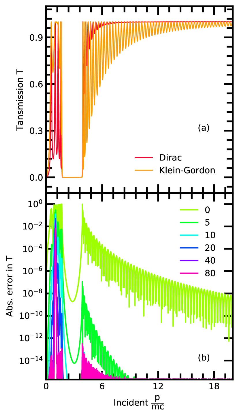
Figure 1: (Color online) (a) Transmission through the potential barrier Eq. (94) as a function of incident momentum $\mathnormal{p}$, for fermions (red) and bosons (orange). (b) Convergence of the fermion transmission with increasing number of relativistic correction Taylor expansion terms $0$, $5$, $10$, $20$, $40$, $80$ as labelled.

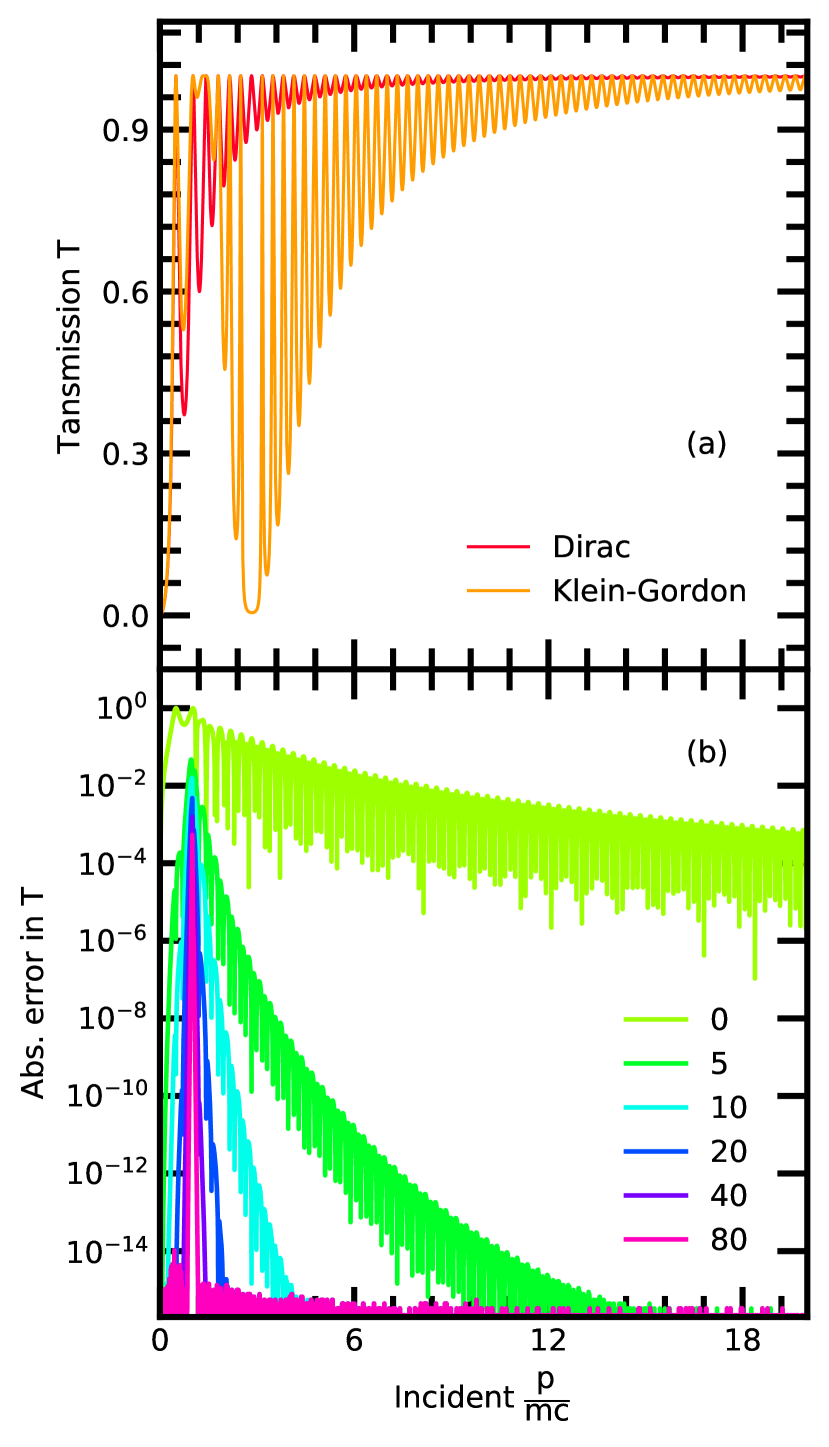
Figure 2: (Color online) Repeat of Fig. 1 except that now electron mass vanishes inside the barrier.

This section is restricted to quantum tunneling. For the structures I investigate in this section I introduce a length scale $a$ given in terms of electron mass $m$, the speed of light $c$, and $\hbar$

$$a=5\dfrac{\hbar}{mc}\,.$$ (93)

In Appendix B I investigate reflection of electrons from a sharp step in potential. In Appendix B I find exact analytic agreement for $R$ between the FW and Dirac spinor representations.

The striking feature of all my results is that I see exact analytic agreement between $T$ and $R$ calculated in the FW and Dirac spinor representations for all momentum $p$, even when $|p|>mc$. This is a significant finding since when $|p|>mc$ the Taylor expansion of $\mathcal{L}$ is a divergent series. I think that conservation of energy is restricting my evaluation of $\mathcal{\accentset{\rule{2.79996pt}{0.7pt}}{L}}$ on $\widetilde{\Psi}^{(\pm)}$ to the particular values required to meet the physical boundary conditions for the Dirac Hamiltonian.

I model a resonant-tunneling diode to compare my WKB approximations of Section 9 and Section 10 as the final example in this section.

For my numerical computations I use Python $3.8$.

14.1 Tunneling through a barrier

The system under consideration is a potential barrier described by

$$V\left(x\right)=-\left\{\begin{array}[]{lc}0&\mbox{for}\ \ \left|x\right|>a\,,\\ 3mc^{2}&\mbox{for}\ \ \left|x\right|<a\,.\end{array}\right.$$ (94)

Since $V$ is negative, the momentum of the electron inside the barrier becomes imaginary when the following condition is met:

$$-mc^{2}<E+V<+mc^{2}\,,$$ (95)

then the electron is quantum tunneling.

The analytic transmission for Eq. (94) is derived in Appendix D as:

$$T\left(k\right)=\dfrac{4\kappa^{2}}{4\kappa^{2}+\left(1-\kappa^{2}\right)^{2}\sin^{2}\left(\dfrac{2mqa}{\hbar}\right)}\,,$$ (96)

where I take $\kappa$ to be $\kappa_{f}$ in the FW representation, and $\kappa_{d}$ in the Dirac spinor representation. For the derivation of Appendix D in the FW representation

$$\kappa^{\left(\pm\right)}_{f}=\dfrac{\alpha^{(\pm)}_{k}}{\alpha^{\left(\pm\right)}_{q}}=\dfrac{q_{x}}{k_{x}}\dfrac{E\pm mc^{2}}{E\pm mc^{2}+V}\,.$$ (97)

It was shown by the authors of Refs. [14, 15] by deriving $T$ in the Dirac spinors representation of quantum tunneling

$$\kappa^{\left(\pm\right)}_{d}=\dfrac{q_{x}}{k_{x}}\dfrac{E\pm mc^{2}}{E\pm mc^{2}+V}\,,$$ (98)

which is in exact analytic agreement with $\kappa^{\left(\pm\right)}_{f}$, as expected.

The numerical results demonstrating relativistic tunneling of electrons are shown in Fig. 1. For comparison I also show the transmission of tunneling bosons with identical mass to the electron.

Fig. 1(b) shows the absolute error calculated as the difference between $T$ evaluated using the Taylor expansions $g(k/c)$ in $\kappa$ or the Python $3.8$ $cmath$ module square root function.

The region of slow convergence around $|k/c|=1$ in Fig. 1(b) is an artifact of the point in $g(k/c)$ about which I have taken my Taylor expansions.

14.2 Tunneling through a barrier with vanishing electron mass inside the barrier

In this subsection I almost repeat the demonstration of Section 14.1 except that now inside the barrier the electron mass is strictly vanishing.

Since $m=0$ when $|x|<a$ I must re-evaluate $\kappa_{d}$ for Eq. (96):

$$\kappa^{\left(\pm\right)}_{d}=\dfrac{q_{x}}{p_{x}}\dfrac{E\pm mc^{2}}{E+V}\,,$$ (99)

which is in exact analytic agreement with $\kappa^{\left(\pm\right)}_{f}$, as expected.

The numerical results demonstrating tunneling of relativistic electrons are shown in Fig. 2. For comparison I also show the transmission of tunneling bosons with identical mass to the electron.

In Fig. 2(b) the absolute error is calculated as the difference between $T$ evaluated using the Taylor expansions $g(k/c)$ in $\kappa$ or the Python $3.8$ $cmath$ module square root function.

The region of slow convergence around $|k/c|=1$ in Fig. 2(b) is an artifact of the point in $g(k/c)$ about which I have taken my Taylor expansions.

14.3 Transmission through a resonant-tunneling diode using the WKB approximation

I calculate the transmission through a resonant diode under a range of bias potentials $\Delta V$. I show a series of potentials describing increasing $\Delta V$ in Fig. 3(a). The transmission as a function of $\Delta V$ is given in Fig. 3(b) for a series of incident energies. I calculate transmission with the two different WKB approximations, derived in Section 9 and Section 10, for comparison in Fig. 3(c).

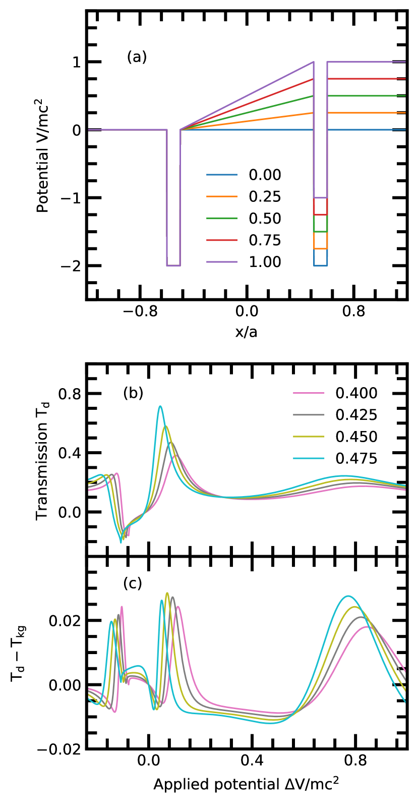
Figure 3: (color online) (a) Potential profile for a representation of a resonant-tunneling diode under a range of bias potentials $\Delta V/mc^{2}$ 0.00, 0.25, 0.50, 0.75, 1.00 as labelled. (b) Transmission as a function of bias potential $\Delta V$ for a series of left hand side electron incident energies $E^{(i)}/mc^{2}$ 0.400, 0.425, 0.450, 0.475 as labelled, with $\Gamma_{i}$ taken to be $\pm\alpha^{\left(\pm\right)}_{i}$. (c) Difference in transmission, as a function of bias potential $\Delta V$, between using $\pm\alpha^{\left(\pm\right)}_{i}$ or $p_{i}$ for $\Gamma_{i}$.

The resonant-tunneling diode that I consider includes a planar cavity with a smoothly varying potential. For the wavefunction to traverse the cavity the employment of WKB transfer matrices developed in Section 9 and Section 10 are required:

$$\begin{pmatrix}\dfrac{\exp{\left(-\dfrac{i}{\hbar}\int^{x_{1}}_{x_{0}}pdx\right)}}{\sqrt{\nicefrac{{\Gamma_{0}}}{{\Gamma_{1}}}}}&0\\ 0&\dfrac{\exp{\left(+\dfrac{i}{\hbar}\int^{x_{1}}_{x_{0}}pdx\right)}}{\sqrt{\nicefrac{{\Gamma_{1}}}{{\Gamma_{0}}}}}\end{pmatrix}\begin{pmatrix}\widetilde{a}_{1}\\ \widetilde{b}_{1}\end{pmatrix}=\begin{pmatrix}\widetilde{a}_{0}\\ \widetilde{b}_{0}\end{pmatrix}\,,$$ (100)

$\Gamma_{i}$ is $p_{i}$ or $\pm\alpha^{\left(\pm\right)}_{i}$ depending on whether I use FW Eq. (16) or Eq. (18) inside the cavity. The subscript $0$ denotes evaluation at $x_{0}=-a/2$ the left hand side of the smoothly varying region for which the transfer matrix is applied, $1$ is at $x_{1}=+a/2$ the right hand side of the smoothly varying region. I define $\widetilde{a}_{0}$, $\widetilde{a}_{1}$, $\widetilde{b}_{0}$, and $\widetilde{b}_{1}$ in the same way as Section 5.

Since I have established in Section 14.1 and Section 14.2 that the Taylor series for $g(k/c)$ gives convergence to the square root function of the Python $3.8$ $cmath$ module, I dispense with the Taylor series and use the $cmath$ square root function to calculate the results in this subsection.

I see in Fig. 3(b) and (c) that as the energy of the incident electrons moves to higher values the first resonance of the diode moves towards lower values of $\Delta V$, as expected. I observe in Fig. 3(b) negative transmission as expected according to the Klein paradox [14, 16].

In Fig. 3(b) and (c) I see no qualitative difference between my two WKB approximations, showing that exponential decay is the dominant factor in the cavity for this example.

15 Conclusion

In this work I have developed Dirac fermion transfer matrix methods, for all energies, in the FW representations. I have also developed WKB approximations, to all orders, and discussed the validity of the approximations. I have introduced connection formulae between regions of real and imaginary fermion momentum.

I have shown the extension of my method to $2$D periodic structures for band engineering [1, 2, 3].

I have alerted the reader to the limits of my methods by revealing a GF paradox that occurs when transforming between Dirac and FW representations.

I have verified my methods for massive and effectively massless fermions of all momentum by analytic comparison with the Dirac spinor representation of fermion tunneling. I have shown that the FW representation is an exact description of Dirac fermions and is not restricted to semi-relativistic energies as first envisioned [11].

16 Acknowledgements

This research was not funded by any research council grants, if you want to help support this research please make a donation: https://gofund.me/34294631. Thank you in advance for whatever you donate.

Future developments will involve the inclusion of RSE perturbation theory [17, 18, 19, 20, 21]. I plan to extend the derivation of the normalization which I made in Ref. [18] to Dirac fermions described by the FW Eq. (18). I acknowledge that as a sub-sequence to my rigorous normalization derivations in Ref. [18], E. A. Muljarov incorporated his zero frequency mode discovery into the generalized normalization. I acknowledge the first of the RSE waveguide articles, which I reference, was predominantly the work of E. A. Muljarov.

17 Declaration of competing interests

I declare that I have no competing financial interests or personal relationships that could have influenced the work reported in this article.

Appendix A Discussion of commutation

In this appendix I will provide a discussion of

$$\mathcal{L}=-\mathcal{\accentset{\rule{2.79996pt}{0.7pt}}{L}}c\hat{p}_{x}=-c\hat{p}_{x}\mathcal{\accentset{\rule{2.79996pt}{0.7pt}}{L}}\,.$$ (101)

Consider the form of the operator $\mathcal{L}$

$$\ \mathcal{L}=mc^{2}\left[\dfrac{1}{2}\left[{\dfrac{\hat{p}}{mc}}\right]^{2}-\dfrac{1}{8}\left[{\dfrac{\hat{p}}{mc}}\right]^{4}+\dfrac{1}{16}\left[{\dfrac{\hat{p}}{mc}}\right]^{6}-...\right]\,,$$ (102)

where

$$\dfrac{1}{2}\left[{\dfrac{\hat{p}}{mc}}\right]^{2}=-\dfrac{\hbar^{2}}{2m^{2}c^{2}}\left[\dfrac{d^{2}}{dx^{2}}+\dfrac{d^{2}}{dy^{2}}\right]\,,$$ (103)

$$\dfrac{1}{8}\left[{\dfrac{\hat{p}}{mc}}\right]^{4}=\dfrac{\hbar^{4}}{8m^{4}c^{4}}\left[\dfrac{d^{4}}{dx^{4}}+2\dfrac{d^{4}}{dy^{2}dx^{2}}+\dfrac{d^{4}}{dy^{4}}\right]\,,$$ (104)

and the series of polynomial differential operators continues up to $n^{th}$ order. It is clear that I can write

$$\dfrac{d^{n+m}}{dx^{n}dy^{m}}=\dfrac{d}{dx}\dfrac{d^{n+m-1}}{dx^{n-1}dy^{m}}=\dfrac{d^{n+m-1}}{dx^{n-1}dy^{m}}\dfrac{d}{dx}\,.$$ (105)

However it is also the case that

$$\dfrac{d^{n}}{dy^{n}}f\left(x,y\right)=\dfrac{d}{dx}\dfrac{dx}{dy}\dfrac{d^{n-1}f}{dy^{n-1}}=\dfrac{d^{n-1}}{dy^{n-1}}\dfrac{dx}{dy}\dfrac{df}{dx}$$ (106)

when every term in $f$ is a function of not just $y$ but also $x$. I see from Eq. (105) and Eq. (106) that I can extract $d/dx$ from either side of the operator $\mathcal{L}$, in these cases.

When $f(x,y)=f(y)$, then in general

$$\dfrac{d^{n}}{dy^{n}}f\left(y\right)\neq 0\,,$$ (107)

but

$$\dfrac{d}{dx}f\left(y\right)=0\,,$$ (108)

therefore in general

$$0\neq\dfrac{d^{n}}{dy^{n}}f\left(y\right)\neq\dfrac{d^{n-1}}{dy^{n-1}}\dfrac{dx}{dy}\dfrac{d}{dx}f\left(y\right)=0\,.$$ (109)

In the case described by Eq. (109) I cannot extract $d/dx$ from either side of the operator $d^{n}/dy^{n}$.

Eq. (101) is true when I assume that $\mathcal{L}$ acts on a function of not just $y$ but also $x$.

Appendix B Reflection at a step potential in Foldy-Wouthuysen and Dirac spinor representations for comparison

Consider a fermion incident on a step at $x=0$. The wavefunction for $x<0$ is

$$\begin{pmatrix}E\pm mc^{2}\\ -cp_{x}\end{pmatrix}\exp{\left(+\dfrac{ip_{x}x}{\hbar}\right)}+B\begin{pmatrix}E\pm mc^{2}\\ +cp_{x}\end{pmatrix}\exp{\left(-\dfrac{ip_{x}x}{\hbar}\right)}\,,$$ (110)

and for $x>0$

$$F\begin{pmatrix}E+V\pm mc^{*2}\\ -c^{*}q_{x}\end{pmatrix}\exp{\left(+\dfrac{iq_{x}x}{\hbar}\right)}\,.$$ (111)

By continuity of wavefunction at $x=0$ I have

$$\big{(}1-B\big{)}cp_{x}=Fc^{*}q_{x}\,,$$ (112)

$$\big{(}1+B\big{)}\big{(}E\pm mc^{2}\big{)}=F\big{(}E+V\pm mc^{*2}\big{)}\,.$$ (113)

Dividing Eq. (112) by Eq. (113) gives

$$\dfrac{1-B}{1+B}=\dfrac{q_{x}c^{*}}{p_{x}c}\dfrac{E\pm mc^{2}}{E+V\pm mc^{*2}}=\kappa^{\left(\pm\right)}_{d}\,.$$ (114)

Now I turn to the FW representation. The corresponding wavefunction for $x<0$ is

$$\exp{\left(+\dfrac{ip_{x}x}{\hbar}\right)}+B\exp{\left(-\dfrac{ip_{x}x}{\hbar}\right)}\,,$$ (115)

and for $x>0$

$$F\exp{\left(+\dfrac{iq_{x}x}{\hbar}\right)}\,.$$ (116)

Applying my boundary condition at $x=0$, continuity of wavefunction and continuity of wavefunction with respect to $\mathcal{\accentset{\rule{2.79996pt}{0.7pt}}{L}}$, I obtain

$$\big{(}1-B\big{)}\alpha^{\left(\pm\right)}_{0}=F\alpha^{\left(\pm\right)}_{1}\,,$$ (117)

$$1+B=F\,.$$ (118)

Dividing Eq. (117) by Eq. (118) gives

$$\dfrac{1-B}{1+B}=\dfrac{\alpha^{\left(\pm\right)}_{1}}{\alpha^{\left(\pm\right)}_{0}}=\dfrac{p_{x}c}{q_{x}c^{*}}\dfrac{E+V\pm mc^{*2}}{E\pm mc^{2}}=\kappa^{\left(\pm\right)}_{f}\,.$$ (119)

In Section 3 I derived $R=|B|^{2}$, therefore

$$R=\left|\dfrac{1-\kappa}{1+\kappa}\right|^{2}\,,$$ (120)

where I use $\kappa^{(\pm)}_{d}$ for the Dirac equation and $\kappa^{\left(\pm\right)}_{f}$ for the FW equation. Substituting either $\kappa^{\left(\pm\right)}_{f}$ or $\kappa^{\left(\pm\right)}_{d}$ into Eq. (120) gives analytically identical $T$ and $R$ between the Dirac and FW representation, as expected. I also calculated $\kappa^{\left(\pm\right)}_{d}$ in the case of $m$ vanishing for $x>0$ to find exact analytic agreement in $T$ and $R$ between the Dirac and FW representations, as expected.

$\kappa^{\left(\pm\right)}_{d}$ corresponds to $\alpha^{\left(\pm\right)}$, and is the mathematical consequence of there being two forms for the FW wavefunction Eq. (18). The FW wavefunction describes the electron $\widetilde{\Psi}^{\left(-\right)}$ or positron $\widetilde{\Psi}^{\left(+\right)}$ [11].

I also calculate, for useful comparison, the transmission of bosons with the following Klein-Gordon result

$$\kappa_{kg}=\dfrac{q_{x}c^{*}}{p_{x}c}\,.$$ (121)

Appendix C Examination of a massless fermion tunneling through a magnetic delta barrier in the Foldy-Wouthuysen representation

Consider a massless fermion tunneling through a magnetic delta barrier $B=B_{0}\delta\left(x\right)\hat{z}$, where $B=\nabla\times A$. The barrier is described by $A=0$ except for $A=A_{y}\hat{y}\neq 0$ when $x>0$. The Dirac spinor wavefunction is a solution of

$$\left[c{\bf\alpha}\cdot\left(\hat{p}-A\right)\right]\Psi=E\Psi\,.$$ (122)

Using the approach of Section 2, Eq. (122) can be transformed to

$$\left[\mp c\sqrt{\left(\hat{p}-A\right)^{2}}\right]\widetilde{\Psi}^{\left(\pm\right)}=E\widetilde{\Psi}^{\left(\pm\right)}\,.$$ (123)

Taylor expanding Eq. (123) around $\hat{p}=0$ gives

$$\left[\mp\mathcal{M}-\left(E\pm cA_{y}\right)\right]\widetilde{\Psi}^{\left(\pm\right)}=0\,,$$ (124)

where $\mathcal{M}$ is the corresponding linear differential operator. Using the approach of Section 4 I calculate, that at the barrier, the wavefunction is continuous and also continuous with respect to $\mathcal{\accentset{\rule{2.79996pt}{0.7pt}}{M}}$, where I define

$$\mathcal{\accentset{\rule{2.79996pt}{0.7pt}}{M}}\widetilde{\Psi}^{\left(\pm\right)}=\pm\dfrac{E\pm cA_{y}}{cp_{x}}\widetilde{\Psi}^{\left(\pm\right)}\,.$$ (125)

I now return to the Dirac spinor representation. In the region $A=A_{y}\hat{y}\neq 0$, the general solution for $\hat{p}=\pm q_{x}\hat{x}$ is given by [22, 23, 24]

$$\Psi=\begin{pmatrix}+E\\ \pm cq_{x}-icA_{y}\end{pmatrix}\exp{\left(\pm\dfrac{iq_{x}x}{\hbar}\right)}\,,$$ (126)

where $cq_{x}=\sqrt{E^{2}-c^{2}A_{y}^{2}}$. The reflection is calculated by matching wavefunctions at the step in vector potential, similar to Appendix C for a step in electrostatic potential.

Making use of my boundary conditions I find the reflection coefficient $R$ takes the form of Eq. (120), with

$$\kappa_{d}=\dfrac{c^{*}}{c}\dfrac{q_{x}-iA_{y}}{p_{x}}$$ (127)

for the Dirac spinor representation and

$$\kappa_{f}=\dfrac{cp_{x}}{c^{*}q_{x}}\dfrac{E\pm c^{*}A_{y}}{E}$$ (128)

for the FW representation. $\hat{p}=p_{x}\hat{x}=(E/c)\hat{x}$ when $A=0$.

The conflict between Eq. (127) and Eq. (128) shows that $R$ calculated in the FW representation does not reproduce $R$ calculated in the Dirac spinor representation, FW wavefunctions cannot be used for the calculation of tunneling through magnetic barriers.

Appendix D Analytic Green’s functions in 1-dimension

Consider

$$\left[\mp\mathcal{L}-\left(V+E\pm mc^{2}\right)\right]G^{\left(\pm\right)}\left(x,x^{\prime}\right)=\delta\left(x-x^{\prime}\right)\,.$$ (129)

Let $\widetilde{\Psi}_{L}$ and $\widetilde{\Psi}_{R}$ be the solutions of Eq. (18) which separately satisfy the boundary conditions at $x=-a$ and $x=+a$. The GF of Eq. (129) for the case of a $1$D barrier can be written as

$$G^{\left(\pm\right)}\left(x,x^{\prime}\right)=\dfrac{\widetilde{\Psi}^{\left(\pm\right)}_{L}\left(x_{<}\right)\widetilde{\Psi}^{\left(\pm\right)}_{R}\left(x_{>}\right)}{\accentset{\rule{2.79996pt}{0.7pt}}{W}^{\left(\pm\right)}}\,,$$ (130)

where $x_{<}=\min{(x,x^{\prime})}$ and $x_{>}=\max{(x,x^{\prime})}$ and

$$\accentset{\rule{2.79996pt}{0.7pt}}{W}^{\left(\pm\right)}=\mp\widetilde{\Psi}^{\left(\pm\right)}_{L}ic\hbar\mathcal{\accentset{\rule{2.79996pt}{0.7pt}}{L}}\widetilde{\Psi}^{\left(\pm\right)}_{R}\pm\widetilde{\Psi}^{\left(\pm\right)}_{R}ic\hbar\mathcal{\accentset{\rule{2.79996pt}{0.7pt}}{L}}\widetilde{\Psi}^{\left(\pm\right)}_{L}$$ (131)

is the Wronskian, which does not depend on $x$.

To prove Eq. (130) and Eq. (131), note that by Eq. (129)

$$\mp\lim_{\epsilon\rightarrow 0}\int^{x^{\prime}+\epsilon}_{x^{\prime}-\epsilon}\mathcal{L}G^{\left(\pm\right)}\left(x,x^{\prime}\right)dx=1\,,$$ (132)

which implies

$$\mp ic\hbar\mathcal{\accentset{\rule{2.79996pt}{0.7pt}}{L}}G^{\left(\pm\right)}\left(x_{+},x^{\prime}\right)\pm ic\hbar\mathcal{\accentset{\rule{2.79996pt}{0.7pt}}{L}}G^{\left(\pm\right)}\left(x_{-},x^{\prime}\right)=1\,,$$ (133)

then, applying $\mathcal{\accentset{\rule{2.79996pt}{0.7pt}}{L}}$ to Eq. (130) written out explicitly

$$\mathcal{\accentset{\rule{2.79996pt}{0.7pt}}{L}}G\left(x,x^{\prime}\right)=\dfrac{1}{\accentset{\rule{2.79996pt}{0.7pt}}{W}}\left\{\begin{array}[]{lc}\mathcal{\accentset{\rule{2.79996pt}{0.7pt}}{L}}\widetilde{\Psi}_{L}\big{(}x\big{)}\widetilde{\Psi}_{R}\big{(}x^{\prime}\big{)}&\mbox{for}\ \ x<x^{\prime}\,,\\ \widetilde{\Psi}_{L}\big{(}x^{\prime}\big{)}\mathcal{\accentset{\rule{2.79996pt}{0.7pt}}{L}}\widetilde{\Psi}_{R}\big{(}x\big{)}&\mbox{for}\ \ x>x^{\prime}\,,\end{array}\right.$$ (134)

and substituting into Eq. (133) gives Eq. (131).

I now calculate the GF for a barrier of width $2a$.

$$\widetilde{\Psi}_{1}=\left\{\begin{array}[]{lll}\exp{\bigg{(}+\dfrac{imkx}{\hbar}\bigg{)}}&x>+a\,,\\ C\exp{\left(+\dfrac{im^{*}qx}{\hbar}\right)}+D\exp{\left(-\dfrac{im^{*}qx}{\hbar}\right)}&\left|x\right|<a\,,\\ A\exp{\bigg{(}+\dfrac{imkx}{\hbar}\bigg{)}}+B\exp{\bigg{(}-\dfrac{imkx}{\hbar}\bigg{)}}&x<-a\,.\end{array}\right.$$ (135)

Continuity of $\Psi_{1}(x)$ and continuity of $\Psi_{1}(x)$ with respect to $\mathcal{\accentset{\rule{2.79996pt}{0.7pt}}{L}}$ gives

$$C=\dfrac{\alpha_{q}+\alpha_{k}}{2\alpha_{q}}\exp{\bigg{(}+\dfrac{imka}{\hbar}\bigg{)}}\exp{\bigg{(}-\dfrac{im^{*}qa}{\hbar}\bigg{)}}\,,$$ (136)

$$D=\dfrac{\alpha_{q}-\alpha_{k}}{2\alpha_{q}}\exp{\bigg{(}+\dfrac{imka}{\hbar}\bigg{)}}\exp{\bigg{(}+\dfrac{im^{*}qa}{\hbar}\bigg{)}}\,.$$ (137)

$\widetilde{\Psi}_{2}$ the left hand solution is given by $\widetilde{\Psi}_{2}(+x)=\widetilde{\Psi}_{1}(-x)$. Therefore the Wronskian is given by

$$\accentset{\rule{2.79996pt}{0.7pt}}{W}=2ic\hbar\alpha_{q}\left(C^{2}-D^{2}\right)\,.$$ (138)

I evaluate Eq. (130) to give $G(+a,-a)$:

$$\dfrac{i\alpha_{q}}{ic\hbar\left(\alpha^{2}_{q}+\alpha^{2}_{k}\right)\sin{\left(\dfrac{2m^{*}qa}{\hbar}\right)}-2c\hbar\alpha_{q}\alpha_{k}\cos{\left(\dfrac{2m^{*}qa}{\hbar}\right)}}\,.$$ (139)

The transmission for a barrier embedded in a vacuum is given as the ratio of $G(+a,-a)$ and the free space GF $G^{fs}(+a,-a)$:

$$T(k)=|2c\hbar\alpha_{k}G\left(+a,-a\right)|^{2}=\left|\dfrac{G\left(+a,-a\right)}{G^{fs}\left(+a,-a\right)}\right|^{2}\,.$$ (140)

The free space GF can be written as

$$\left[\mp\mathcal{L}-\left(E\pm mc^{2}\right)\right]G^{(\pm)}\left(x,x^{\prime}\right)=\delta\left(x-x^{\prime}\right)\,,$$ (141)

therefore by symmetry, when $x^{\prime}=0$,

$$G^{(\pm)}(x,0)=A^{\left(\pm\right)}\left\{\begin{array}[]{lc}\exp{\left(-\dfrac{imkx}{\hbar}\right)}&\mbox{for}\ \ x<0\,,\\ \exp{\left(+\dfrac{imkx}{\hbar}\right)}&\mbox{for}\ \ x>0\,.\end{array}\right.$$ (142)

Integrating Eq. (141) across $\left[0_{-},0_{+}\right]$ gives

$$\mp{i}{c\hbar A^{\left(\pm\right)}}\mathcal{\accentset{\rule{2.79996pt}{0.7pt}}{L}}\exp{\left(+\dfrac{imk0_{+}}{\hbar}\right)}\pm{i}{c\hbar A^{\left(\pm\right)}}\mathcal{\accentset{\rule{2.79996pt}{0.7pt}}{L}}\exp{\left(-\dfrac{imk0_{-}}{\hbar}\right)}=1$$ (143)

and letting $0_{+}\rightarrow 0$ and $0_{-}\rightarrow 0$, I find

$$A^{\left(\pm\right)}=\dfrac{1}{2ic\hbar\alpha^{\left(\pm\right)}_{k}}\,.$$ (144)

Appendix E Green’s function paradox

I reveal a GF paradox occurring when transforming between the FW and Dirac representations.

Let

$$\left[H-\left(E+V\right)\right]\mathcal{G}\left(r,r^{\prime}\right)=\delta\left(r-r^{\prime}\right)\hat{1}\,,$$ (145)

therefore

$$e^{+iS}\left[H-\left(E+V\right)\right]e^{-iS}e^{+iS}\left[\mathcal{G}\left(r,r^{\prime}\right)\right]e^{-iS}\\ =e^{+iS}\hat{1}e^{-iS}\delta\left(r-r^{\prime}\right)\,.$$ (146)

However since

$$e^{+iS}\hat{1}e^{-iS}\delta\left(r-r^{\prime}\right)=\hat{1}\delta\left(r-r^{\prime}\right)\,,$$ (147)

and since I have already seen in Section 2

$$e^{+iS}\left[H-\left(E+V\right)\right]e^{-iS}=\left[\mp\mathcal{L}-\left(V+E\pm mc^{2}\right)\right]\hat{1}\,,$$ (148)

I have

$$e^{+iS}\left[\mathcal{G}\left(r,r^{\prime}\right)\right]e^{-iS}=G^{\left(\pm\right)}\left(r,r^{\prime}\right)\hat{1}\\ \implies e^{-iS}G^{\left(\pm\right)}\left(r,r^{\prime}\right)e^{+iS}=\mathcal{G}\left(r,r^{\prime}\right)\hat{1}\,.$$ (149)

Eqs. (149) imply that the valid GFs of the Dirac equation are diagonal. Now consider the identity

$$\left[H-\left(E+V\right)\right]\left[H+\left(E+V\right)\right]K\left(r,r^{\prime}\right)=\hat{1}\delta\left(r-r^{\prime}\right)\,,$$ (150)

so that

$$\left[H+\left(E+V\right)\right]K\left(r,r^{\prime}\right)=\mathcal{G}\left(r,r^{\prime}\right)\,.$$ (151)

Multiplying out the brackets in Eq. (150) I obtain

$$-c^{2}\hbar^{2}\left[\nabla^{2}+\left(\dfrac{p}{\hbar}\right)^{2}\right]K\left(r,r^{\prime}\right)=\delta\left(r-r^{\prime}\right)\,.$$ (152)

I see from Eq. (152) that in $1$D free space ($V=0$):

$$c^{2}\hbar^{2}K\left(x,x^{\prime}\right)=-\dfrac{\hbar\exp{\left(\dfrac{ip\left|x-x^{\prime}\right|}{\hbar}\right)}}{2ip}\,,$$ (153)

in $2$D free space:

$$c^{2}\hbar^{2}K\left(\rho,\rho^{\prime}\right)=\dfrac{i}{4}H^{(1)}_{0}\left(\dfrac{p\left|\rho-\rho^{\prime}\right|}{\hbar}\right)\,,$$ (154)

and in $3$D free space:

$$c^{2}\hbar^{2}K\left(r,r^{\prime}\right)=\dfrac{\exp{\left(\dfrac{ip\left|r-r^{\prime}\right|}{\hbar}\right)}}{4\pi\left|r-r^{\prime}\right|}\,.$$ (155)

Substituting the identity Eq. (151) into Eq. (149)

$$e^{+iS}\left[H+\left(E+V\right)\right]e^{-iS}K\left(r,r^{\prime}\right)=G^{(\pm)}\left(r,r^{\prime}\right)\hat{1}$$ (156)

and so

$$\left[\sqrt{\hat{p}^{2}c^{2}+m^{2}c^{4}}+\left(E+V\right)\right]K\left(r,r^{\prime}\right)=G^{\left(\pm\right)}\left(r,r^{\prime}\right)\hat{1}\,.$$ (157)

By inspection of Eq. (157) and the energy momentum relation $(E+V)=\sqrt{p^{2}c^{2}+m^{2}c^{4}}$,

$$G^{\left(\pm\right)}\left(r,r^{\prime}\right)=2\left(E+V\right)K\left(r,r^{\prime}\right)$$ (158)

and substituting Eq. (158) into Eq. (149) I also have

$$\mathcal{G}\left(r,r^{\prime}\right)=2\left(E+V\right)K\left(r,r^{\prime}\right)\,.$$ (159)

Eq. (159) is consistent with the relativistic correction to the $1st$ Born approximation in $3$D.

Let us test Eq. (158) and Eq. (159) by making an analytic comparison between the GF for $1$D free space Eq. (142) and the GF composed of Eq. (159) and Eq. (153):

$$2EK=-E\dfrac{\exp{\left(\dfrac{ip\left|x-x^{\prime}\right|}{\hbar}\right)}}{i\hbar pc^{2}}\neq\dfrac{\exp{\left(\dfrac{ip\left|x-x^{\prime}\right|}{\hbar}\right)}}{2ic\hbar\alpha_{k}}$$ (160)

and so I have an apparent paradox.

Let us attempt to resolve the paradox. I have shown in Appendix D that there are two possible forms of the FW GF:

$$G^{\left(\pm\right)}\left(x,x^{\prime}\right)=\dfrac{\exp{\left(\dfrac{ip\left|x-x^{\prime}\right|}{\hbar}\right)}}{2ic\hbar\alpha^{\left(\pm\right)}_{k}}$$ (161)

for an electron delta source ($-$) or a positron source ($+$). If I add my two expressions $G^{(\pm)}(x,x^{\prime})$ I find

$$G^{\left(-\right)}\left(x,x^{\prime}\right)+G^{\left(+\right)}\left(x,x^{\prime}\right)=2EK\left(x,x^{\prime}\right)\,.$$ (162)

However if I try to prove that in general

$$\mathcal{G}\left(r,r^{\prime}\right)=G^{\left(-\right)}\left(r,r^{\prime}\right)+G^{\left(+\right)}\left(r,r^{\prime}\right)\,,$$ (163)

I arrive at a contradiction. The Klein-Gordon GF has the continuity conditions of the Klein-Gordon equation, $(E+V)$ can be a discontinuous function, therefore $2(E+V)K$ can be discontinuous at boundaries. Therefore Eq. (159) implies $\mathcal{G}$ may be discontinuous. $\mathcal{G}$ has the same boundary conditions as $\Psi$, Eq. (159) may violate the boundary conditions for $\mathcal{G}$.

Let us now discuss a possible cause of the paradox. To evaluate the FW transformations defined to be

$$e^{\pm iS}=\cos\theta\pm{\bf\beta}{\bf\alpha}\cdot\dfrac{\hat{p}}{|\hat{p}|}\sin\theta\,,$$ (164)

I am required to know the momentum $\hat{p}$ also at the delta source. To make this calculation of $\hat{p}$ at the delta source consider Eq. (142) from Appendix D,

$$G\left(x,0\right)=\dfrac{1}{2ic\hbar\alpha_{k}}\left\{\begin{array}[]{lc}\exp{\left(-\dfrac{imkx}{\hbar}\right)}&\mbox{for}\ \ x<0\,,\\ \exp{\left(+\dfrac{imkx}{\hbar}\right)}&\mbox{for}\ \ x>0\,.\end{array}\right.$$ (165)

I see from Eq. (165) that

$$p_{x}\left(x=0\right)G\left(x,0\right)=\lim_{0_{\pm}\rightarrow 0}\hat{p}G\left(0_{\pm},0\right)={\pm}mkG\left(0,0\right)\,.$$ (166)

Eq. (166) indicates that when $x=x^{\prime}$, the momentum $\hat{p}$ is undefined. Therefore at the delta source the FW transformation is undefined. In $1$D it might be impossible to evaluate $e^{\pm iS}$ at the delta source.

References

• Barbier et al. [2010] M. Barbier, P. Vasilopoulos, F. Peeters, Extra dirac points in the energy spectrum for superlattices on single-layer graphene, Physical Review B 81 (2010) 075438. doi:https://doi.org/10.1103/PhysRevB.81.075438.
• Barbier et al. [2008] M. Barbier, F. Peeters, P. Vasilopoulos, J. M. Pereira, Dirac and klein-gordon particles in one-dimensional periodic potentials, Phys. Rev. B 77 (2008) 115446. doi:https://doi.org/10.1103/PhysRevB.77.115446.
• Arovas et al. [2010] D. Arovas, L. Brey, H. Fertig, E.-A. Kim, K. Ziegler, Dirac spectrum in piecewise constant one-dimensional (1d) potentials, New Journal of Physics 12 (2010) 123020. doi:https://doi.org/10.1088/1367-2630/12/12/123020.
• Guinea et al. [2010] F. Guinea, M. Katsnelson, A. Geim, Energy gaps and a zero-field quantum hall effect in graphene by strain engineering, Nature Physics 6 (2010) 30–33. doi:https://doi.org/10.1038/nphys1420.
• Novoselov et al. [2016] K. S. Novoselov, A. Mishchenko, A. Carvalho, A. H. C. Neto, 2d materials and van der waals heterostructures, Science 353 (2016). doi:https://doi.org/10.1126/science.aac9439.
• Wan et al. [2015] C. Wan, X. Gu, F. Dang, T. Itoh, Y. Wang, H. Sasaki, M. Kondo, K. Koga, K. Yabuki, G. J. Snyder, et al., Flexible n-type thermoelectric materials by organic intercalation of layered transition metal dichalcogenide tis 2, Nature materials 14 (2015) 622–627. doi:https://doi.org/10.1038/nmat4251.
• Song et al. [2013] Y. Song, H.-C. Wu, Y. Guo, Negative differential resistances in graphene double barrier resonant tunneling diodes, Applied Physics Letters 102 (2013) 093118. doi:https://doi.org/10.1063/1.4794952.
• Sonin [2009] E. Sonin, Effect of klein tunneling on conductance and shot noise in ballistic graphene, Physical Review B 79 (2009) 195438. doi:https://doi.org/10.1103/PhysRevB.79.195438.
• Tudorovskiy et al. [2012] T. Tudorovskiy, K. Reijnders, M. I. Katsnelson, Chiral tunneling in single-layer and bilayer graphene, Physica Scripta 2012 (2012) 014010. doi:https://doi.org/10.1088/0031-8949/2012/T146/014010.
• Zalipaev et al. [2015] V. Zalipaev, C. Linton, M. Croitoru, A. Vagov, Resonant tunneling and localized states in a graphene monolayer with a mass gap, Physical Review B 91 (2015) 085405. doi:https://doi.org/10.1103/PhysRevB.91.085405.
• Foldy and Wouthuysen [1950] L. L. Foldy, S. A. Wouthuysen, On the dirac theory of spin 1/2 particles and its non-relativistic limit, Physical Review 78 (1950) 29. doi:https://doi.org/10.1103/PhysRev.78.29.
• Ko and Sambles [1988] D. Y. K. Ko, J. Sambles, Scattering matrix method for propagation of radiation in stratified media: attenuated total reflection studies of liquid crystals, JOSA A 5 (1988) 1863–1866. doi:https://doi.org/10.1364/JOSAA.5.001863.
• Tikhodeev et al. [2002] S. G. Tikhodeev, A. L. Yablonskii, E. A. Muljarov, N. A. Gippius, T. Ishihara, Quasiguided modes and optical properties of photonic crystal slabs, Phys. Rev. B 66 (2002) 045102. URL: https://link.aps.org/doi/10.1103/PhysRevB.66.045102. doi:10.1103/PhysRevB.66.045102.
• Calogeracos and Dombey [1999] A. Calogeracos, N. Dombey, History and physics of the klein paradox, Contemporary physics 40 (1999) 313–321. doi:https://doi.org/10.1080/001075199181387.
• Dosch et al. [1971] H. Dosch, V. Muller, J. Jensen, Kleins paradox, Physica Norvegica 5 (1971) 151.
• Klein [1929] O. Klein, Die reflexion von elektronen an einem potentialsprung nach der relativistischen dynamik von dirac, Zeitschrift für Physik 53 (1929) 157–165. doi:https://doi.org/10.1007/BF01339716.
• Muljarov et al. [2011] E. A. Muljarov, W. Langbein, R. Zimmermann, Brillouin-wigner perturbation theory in open electromagnetic systems, EPL (Europhysics Letters) 92 (2011) 50010. doi:https://doi.org/10.1209/0295-5075/92/50010.
• Doost et al. [2014] M. B. Doost, W. Langbein, E. A. Muljarov, Resonant-state expansion applied to three-dimensional open optical systems, Physical Review A 90 (2014) 013834. doi:https://doi.org/10.1103/PhysRevA.90.013834.
• Armitage et al. [2014] L. J. Armitage, M. B. Doost, W. Langbein, E. A. Muljarov, Resonant-state expansion applied to planar waveguides, Physical Review A 89 (2014) 053832. doi:https://doi.org/10.1103/PhysRevA.89.053832.
• Doost [2016a] M. B. Doost, Resonant-state-expansion born approximation with a correct eigen-mode normalisation, Journal of Optics 18 (2016a) 085607. doi:https://doi.org/10.1088/2040-8978/18/8/085607.
• Doost [2016b] M. B. Doost, Resonant-state-expansion born approximation for waveguides with dispersion, Physical Review A 93 (2016b) 023835. doi:https://doi.org/10.1103/PhysRevA.93.023835.
• Masir et al. [2008a] M. R. Masir, P. Vasilopoulos, A. Matulis, F. Peeters, Direction-dependent tunneling through nanostructured magnetic barriers in graphene, Physical Review B 77 (2008a) 235443. doi:https://doi.org/10.1103/PhysRevB.77.235443.
• Masir et al. [2008b] M. R. Masir, P. Vasilopoulos, F. Peeters, Wavevector filtering through single-layer and bilayer graphene with magnetic barrier structures, Applied Physics Letters 93 (2008b) 242103. doi:https://doi.org/10.1063/1.3049600.
• Masir et al. [2009] M. R. Masir, P. Vasilopoulos, F. Peeters, Magnetic kronig–penney model for dirac electrons in single-layer graphene, New Journal of Physics 11 (2009) 095009. doi:https://doi.org/10.1088/1367-2630/11/9/095009.