Abstract

Achievable rates of the nonlinear frequency-division multiplexing (NFDM) and wavelength-division multiplexing (WDM) subject to the same power and bandwidth constraints are computed as a function of transmit power in the standard single-mode fiber. NFDM achieves higher rates than WDM.

OCIS codes:  060.2330, 060.4370

1 Introduction

The achievable rates of the linear and nonlinear frequency-division multiplexing (NFDM) were compared in fibers with normal dispersion in [1]. In this case, the discrete eigenvalues are naturally absent in the nonlinear Fourier transform (NFT). It was shown that the NFDM rate increases monotonically with transmit power in simulations, while the rates of the wavelength-division multiplexing (WDM) characteristically vanish at an optimal power.

In this paper, we generalize the results of [1] from normal dispersion fiber (defocusing regime, with negative dispersion $D$) to the anomalous dispersion fiber (focusing regime, with positive dispersion $D$). In the focusing regime, solitons can be present. However, we set the discrete spectrum to zero and modulate merely the continuous spectrum in the NFT. We assume a network scenario, defined formally in [1, Section II. A], and compare the achievable rates of the NFDM and WDM subject to the same power and bandwidth constraints.

The continuous spectrum modulation is studied in [2, Part III, Section V. D], [3, 4, 5, 6, 7]. However, nonlinear signal multiplexing, the main ingredient in NFDM responsible for high data rates, was not realized until recently in the defocusing regime, where the NFT simplifies [1]. Following [1], the authors of [8] considered nonlinear multiplexing in multi-user systems in the focusing regime. However, computation of the spectral efficiency (SE), taking into account time duration and bandwidth, and its comparison with the SE of the WDM under the same constraints is lacking. In this paper, we undertake such study.

In Section 2, we recall a few equations from [1] that are used in this paper. The achievable rates of NFDM and WDM are computed in Section 2. In Section 4, we comment on nonlinear multiplexing in the focusing and de-focusing regimes.

2 Nonlinear Frequency-Division Multiplexing

Signal propagation in single-mode optical fiber with distributed amplification is modeled by the stochastic nonlinear Schrödinger (NLS) equation. The equation can be normalized as [2, Eq. 3]

$$j\frac{\partial q}{\partial z}=\frac{\partial^{2}q}{\partial t^{2}}+2|q|^{2}q+n(t,z),\ \ 0\leq z\leq\mathcal{L},$$

where $q(t,z)$ is the complex envelope of the signal as a function of time $t$ and distance $z$ and $n(t,z)$ is zero-mean white circularly-symmetric Gaussian noise.

Consider a multi-user system with $N_{u}$ users, each sending $N_{s}$ symbols, with total (linear) bandwidth $B$ Hz and (total) average power $\mathcal{P}$. Let $\lambda\in\mathbb{R}$ be the generalized frequency, in Fourier transform relation with the generalized time $\tau$. The NFDM transmitter (TX) consists of three steps. In the first step, the following function is computed

$$u(\tau,0)=\sqrt{2}\sum_{k=-\frac{N_{u}}{2}}^{\frac{N_{u}}{2}-1}\sum_{\ell=-\frac{N_{s}}{2}}^{\frac{N_{s}}{2}-1}s^{k}_{\ell}\phi(\tau-\ell T_{0})e^{j2\pi kW_{0}\tau},$$ (1)

where $\phi(\tau)$ is a root-raised-cosine function with the bandwidth $W_{0}$ Hz and the roll-off factor $r$, $T_{0}=1/W_{0}$, and $\{s_{l}^{k}\}_{l}$ are symbols of user $k$ chosen from a constellation $\Xi$.

In the second step, the transmit signal in the nonlinear Fourier domain is calculated

$$\hat{q}(\lambda,0)=\Bigl{(}e^{|U(\lambda,0)|^{2}}-1\Bigr{)}^{\frac{1}{2}}e^{j\angle U(\lambda,0)},$$

in which $U(\lambda,0)=\mathcal{F}(u(\tau,0))/\sqrt{2}$, where $\mathcal{F}$ denotes Fourier transform. Finally, $q(t,0)=\textnormal{INFT}(\hat{q}(\lambda,0))$.

The NFDM receiver (RX) similarly consists of three steps. In the first step, the forward NFT is applied to obtain $\hat{q}(\lambda,\mathcal{L})=\textnormal{NFT}(q(t,\mathcal{L}))$. In the second step, first channel equalization is performed

$$\hat{q}(\lambda,0)=\hat{q}(\lambda,\mathcal{L})e^{4j\lambda^{2}\mathcal{L}};$$

then the $U$ function is computed

$$U(\lambda,\mathcal{L})=\Bigl{(}\log\bigl{(}1+|\hat{q}(\lambda,0)|^{2}\bigr{)}\Bigr{)}^{\frac{1}{2}}e^{j\angle\hat{q}(\lambda,0)}.$$

In the third step, received symbols are obtained by match filtering

$$s^{k}_{\ell}=\int_{-\infty}^{\infty}u(\tau,\mathcal{L})\phi^{*}(\tau-\ell T_{0})e^{-2\pi jkW_{0}\tau}d\tau,$$

where $u(\tau,\mathcal{L})=\sqrt{2}\mathcal{F}^{-1}(U(\lambda,\mathcal{L}))$.

Constellation $\Xi$ and the nonlinear bandwidth $W_{0}$ are chosen so that the linear bandwidth of $q(t,z)$ is $B$ Hz.

3 Achievable Rates of the NFDM and WDM

We consider $N_{u}=5$, $N_{s}=1$, $B=100$ GHz, $\mathcal{L}=2000$ km, $r=25\%$ and fiber parameters in [2, Part III, Table I]. One nonlinear multiplexer at the input, and one nonlinear de-multiplexer at the output, are implemented in the NFDM. The same setup is considered for WDM. The equalization in WDM is applying back-propagation to the central user. In this paper, bandwidth and time duration of the signals are defined as the intervals that contain 99% of the signal energy.

The constellation $\Xi$ consists of $32<N_{r}<64$ rings with $N_{\phi}=128$ phase points in each ring. The number of samples in time, linear and nonlinear frequency is $N=2^{14}$. We compute the transition probabilities for the central symbol in the central user $s^{0}_{0}\rightarrow\hat{s}^{0}_{0}$ based on 4500 noise realizations. The mutual information is maximized using the Arimoto-Blahut algorithm. The resulting rates as a function of the launch power are plotted in Fig. 1 (a). It can be observed that, while the WDM rates rolls off near $\mathcal{P}=-4.5$ dBm, the NFDM increases for the range of power shown in Fig. 1 (a).

The data rates shown in Fig. 1 (a) are measured in bits per two real dimensions (bits/2D). They can be converted to the spectral efficiency (SE) by dividing bits/2D by $\alpha=B_{\max}T_{a}/(N_{u}N_{s})$, where $T_{a}$ is the average time duration of the signal set at the input and $B_{\max}$ is the maximum input output bandwidth. Asymptotically as the transmission time tends to infinity, $\alpha\rightarrow 1$ so that the rates shown in Fig. 1 (a) represent SE. In the finite-blocklength regime with $N_{s}=1$, to give an example, the SE of the NFDM and WDM at $\mathcal{P}=3.5$ dBm are, respectively, 1.81 and 1.31 bits/s/Hz

Note that the signal power defined based on the $99\%$ time duration may not be a good definition for capacity. The rates shown in Fig. 1 (a) could change using different signals with the same power. Nevertheless, $\max R_{\textnormal{WDM}}(\mathcal{P})<\max R_{\textnormal{NFDM}}(\mathcal{P})$. More work is needed for a comprehensive comparison.

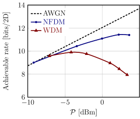
    (a)        (b)        (c)

Fig. 1: (a) Achievable rates of the NFDM and WDM. Transmit and received symbols in (b) NFDM and (c) WDM, at the same power $\mathcal{P}=3.5$ dBm.

4 Stochastic Memory

Consider the mutual information for the central user $s_{0}^{0}\mapsto\{\hat{s}_{l}^{0}\}_{l}$. Using the chain rule for the mutual information

$$I\bigl{(}s_{0}^{0};\{\hat{s}_{l}^{0}\}_{l}\bigr{)}=I\bigl{(}s_{0}^{0};\hat{s}_{0}^{0}\bigr{)}+\underbrace{I\bigl{(}s_{0}^{0};\{\hat{s}_{l}^{0}\}_{l\neq 0}|\hat{s}_{0}^{0}\bigr{)}}_{\textnormal{stochastic memory}}.$$ (2)

In the absence of noise there is no memory, i.e., $\hat{s}_{0}^{0}=s_{0}^{0}$ and $\hat{s}_{l}^{0}=0$, $l\neq 0$. Noise, however, causes information to flow from $s_{0}^{0}$ to $\hat{s}_{l}^{0}$ for all $l$, so that the second term in (2) is non-zero. This term, which we call the stochastic memory, is ignored in our simulations. As a consequence, the rates shown in Fig. 1 (a) are lower bounds to the corresponding maximum achievable rates.

From the conservation of energy, when the memory is large, $|\hat{s}_{0}^{0}|<|s_{0}^{0}|$, i.e., the received symbols cluster in a cloud that is closer to origin than $s_{0}^{0}$. Limiting the detection at the RX to $\hat{s}_{0}^{0}$ results in an output SNR loss. We observed that, as the input power is increased, the stochastic memory grows and the output SNR is decreased. This is one reason that the NFDM lower bound in Fig.  1 (a) saturates at high powers: we do not account for all received symbols. The stochastic memory exists in WDM with back-propagation as well. Compared with the defocusing regime, continuous spectrum modulation in the focusing regime produces signals with larger peak-to-average ratio and stochastic memory.

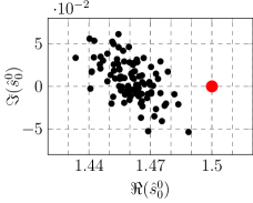
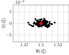
            (a)             (b)              (c)

Fig. 2: Transmit and received symbols in the (a) defocusing regime, (b) focusing regime, and (c) the AWGN channel. Here, $B=60$ GHz, $N_{u}=5$ and $s_{0}^{0}=0.5$. Transmit energy is the same in all cases.

- [1] M. I. Yousefi, et al., “Linear and nonlinear frequency-division multiplexing,” arXiv:1603.04389 (2016).
- [2] M. I. Yousefi, et al., “Information transmission using the nonlinear Fourier transform, Part I, II, III,” IEEE Trans. Inf. Theory 60, 4312–4369 (2014).
- [3] J. E. Prilepsky, et al., “Nonlinear spectral management: Linearization of the lossless fiber channel,” Opt. Exp. 21, 24344–24367 (2013).
- [4] S. T. Le, et al., “Nonlinear inverse synthesis for high spectral efficiency transmission in optical fibers,” Opt. Exp. 22, 26720–26741 (2014).
- [5] S. Wahls, et al., “Digital backpropagation in the nonlinear Fourier domain,” in IEEE Int. Workshop Signal Process. Advances Wireless Commun., Stockholm, Sweden (2015), pp. 445–449.
- [6] V. Aref, et al., “Demonstration of fully nonlinear spectrum modulated system in the highly nonlinear optical transmission regime,” in European Conf. Opt. Commun., Düsseldorf, Germany (2016), pp. 19–21.
- [7] I. Tavakkolnia, et al., “Signalling over nonlinear fibre-optic channels by utilizing both solitonic and radiative spectra,” in European Conf. Networks and Commun., Paris, France (2015), pp. 103–107.
- [8] S. A. Derevyanko, et al., “Capacity estimates for optical transmission based on the nonlinear Fourier transform,” Nature Commun. 7, 12710 (1–9), (2016).