Local Subspace-Based Outlier Detection using Global Neighbourhoods
Abstract
Outlier detection in high-dimensional data is a challenging yet important task, as it has applications in, e.g., fraud detection and quality control. State-of-the-art density-based algorithms perform well because they 1) take the local neighbourhoods of data points into account and 2) consider feature subspaces. In highly complex and high-dimensional data, however, existing methods are likely to overlook important outliers because they do not explicitly take into account that the data is often a mixture distribution of multiple components.
We therefore introduce Gloss, an algorithm that performs local subspace outlier detection using global neighbourhoods. Experiments on synthetic data demonstrate that Gloss more accurately detects local outliers in mixed data than its competitors. Moreover, experiments on real-world data show that our approach identifies relevant outliers overlooked by existing methods, confirming that one should keep an eye on the global perspective even when doing local outlier detection.
I Introduction
Outlier detection [1] is an important task that has applications in many domains. In fraud detection, for example, a bank could be interested in detecting fraudulent transactions; in network intrusion detection, it could be of interest to automatically detect suspicious network events; in a manufacturing plant, identifying raw materials or products with strongly deviating properties could be useful as part of quality control. In each of these applications, the data is high-dimensional and each data point is a potential outlier.
Many techniques for outlier detection have been proposed and studied. Many traditional outlier detection methods [2] are parametric and thus make strong assumptions about the data. Moreover, data points are always considered as a whole and relative to all other data points, which strongly limits the accuracy of these methods on high-dimensional data. Outlier detection in complex, high-dimensional data is an inherently hard problem, as data points tend to have similar distances due to the infamous ‘curse of dimensionality’. To address both this problem and the limitations of (global) outlier detection, local outlier detection methods [3, 4, 5] have been proposed over the past few decades. These methods are distance- or density-based, and assign outlier scores based on the distance of a data point to its closest neighbours relative to the local density of its neighbourhood. To further improve on this, local subspace outlier detection methods [6, 7, 8] have been introduced. They search for local outliers within so-called subspaces, i.e., subsets of the complete set of features. This results in each outlier being reported together with a corresponding subspace in which it is far away from its neighbours. Existing local outlier detection approaches, however, are bound to overlook outliers when the data is a mixture of high-dimensional data points drawn from different data distributions. That is, as we will show, a local neighbourhood found within a given subspace may very well include data points from different components of the mixture, which might result in clear outliers hiding in the crowd of a different component. This is especially relevant when the individual components of the mixture are unknown and hence the dataset has to be analysed as a whole.
We encountered this exact situation in an ongoing collaboration with the BMW Group, where our aim is to identify steel coils strongly deviating in terms of their material properties. The data is very high-dimensional, as it contains hundreds of measurements per coil, but is also known to be a mixture of samples from different distributions: the steel coils have different grades and come from different suppliers. Unfortunately, part of this information is not available in the data and we therefore had to analyse the complete, mixed data. However, what is a ‘normal’ measurement for one type of coil can be a clear deviation for another type of coil; therefore, existing outlier detection methods did not perform well. Subsection VI-D will show examples of relevant outliers detected by our approach that were not found by existing methods.
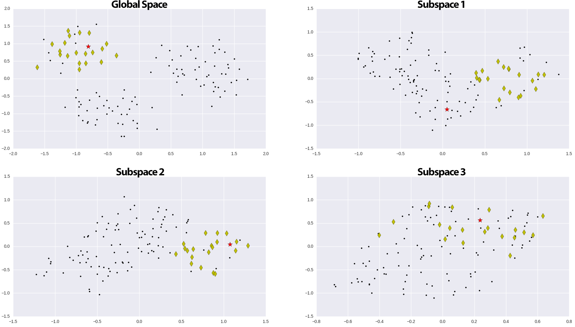
Figure 1 illustrates the problem that we consider on a synthetic dataset. The data consists of three normally distributed clusters in six dimensions; the generative process (and experiments on generated data) will be described in detail in Subsection VI-A. When considering all data points, the data point depicted by the red star is not a local outlier in any of the subspaces, neither in the global nor in any of the two-dimensional subspaces (only three shown). However, when only considering the data point’s neighbours in the global space, here depicted with yellow diamonds, we can observe that the red star is a clear outlier in the 2D subspace shown in the top right plot. it happens to be close to data points from other components, but is far away from data points from the component it belongs to and is therefore an outlier. As we will show in Subsection VI-A, existing algorithms are unable to detect such outliers, especially in high-dimensional data, whereas our method can.
Approach and contributions Our first contribution is the formalisation of the Local Subpace Outlier in Global Neighbourhood problem. That is, we propose to combine local subspace outlier detection with neighbourhoods selected in the global data space. The purpose of using global neighbourhoods is to assess the degree of outlierness of a given data point relative to other data points belonging to the same mixture component, avoiding the possibility that outliers can hide among members of other components of the mixture distribution. Following this, our second contribution is the introduction of the Gloss algorithm, which combines our ideas on outlier detection using global neighbourhoods with techniques from LoOP [5] and HiCS [6].
Given a dataset, it computes the probability that a data point is an outlier according to the problem definition. Moreover, it does so for all feature subspaces deemed relevant and hence also provides information about the subspace(s) in which a data point is considered to be an outlier.
Finally, the third contribution of this paper is an extensive set of experiments on both synthetic and real-world data, in which we evaluate Gloss and compare its performance to its state-of-the-art competitors. The experiments demonstrate that the use of global neighbourhoods enable the discovery of outliers that would otherwise be left undetected, without sacrificing detection accuracy on ‘regular’ outliers. Moreover, global neighbourhoods give Gloss an edge in terms of computational efficiency. Finally, Gloss identifies relevant outliers on real-world manufacturing data from the BMW Group that are not marked as such by existing methods. This confirms that outliers can indeed be hidden in mixture distributions in real-world applications and that taking this into account results in better outlier detection.
II Related Work
Although most previous work on outlier detection has been done in statistics, there are also clustering-based [9], nearest neighbour-based [10], classification-based [11] and spectral-based [12] outlier detection algorithms. Statistical approaches can be categorised as: distribution-based [2], where a standard distribution is used to fit the data; distance-based [13], where the distance to neighbouring points are used to classify outliers versus non-outliers; and density-based, where the density of a group of points is estimated to determine an outlier score. While classification, clustering- and distribution-based algorithms aim to find global outliers by comparing each data point to (a representation of) the complete dataset, distance- and density-based algorithms detect local outliers. We next describe the methods most relevant to our paper:
Local Outlier Factor (LOF) [3] was the first algorithm to introduce the concept of local density to identify outliers. The authors also claim that they are the first to use a (continuous) ‘outlier factor’ rather than a Boolean outlier class.
The LOF algorithm uses a user-defined parameter, MinPts, that determines the local neighbourhood used for computing the outlier factor for each data point. The outcome of the algorithm strongly depends on this setting. One of the disadvantages of the LOF algorithm is that it is hard to tune the MinPts parameter. Quite some modifications and/or enhancements of LOF, such as the Incremental Local Outlier Factor (ILOF) [14] algorithm, have been proposed. ILOF is a modification of LOF that can handle large data streams and compute local outlier factors on-the-fly. It also updates the profiles of already calculated data points since the profiles may change over time.
Local Correlation Integral (LOCI) [4] detects outliers and groups of outliers (small clusters) using the multi-granularity deviation factor (MDEF). If a point differs more than three standard deviations from the local average MDEF, it is labelled as outlier. This method uses two neighbourhood definitions: one neighbourhood to use for the average granularity (density) and one neighbourhood for the local granularity of a given point. The setting of these and determines the complexity and accuracy of the algorithm. Typically is set to and is set in such way that it always covers at least neighbours.
Local Outlier Probabilities (LoOP) [5] is also similar to LOF but does not provide an outlier factor. Instead, it provides the probability of a point being an outlier using the probabilistic set distance of a point to its nearest neighbours. Given this distance and the distances of its neighbours, a Probabilistic Local Outlier Factor (PLOF) is computed and normalised. We will build upon LoOP in this paper.
Subspace Outlier Detection (SOD) [7] is an algorithm that searches for outliers in meaningful subspaces of the data space or even in arbitrarily-oriented subspaces [8]. Other work in the area of spatial data uses special spatial attributes to define neighbourhood and usually one other attribute to find outliers that deviate in this attribute given its spatial neighbours [15, 16].111More details and a comparison of these algorithms can be found in [17].
Outlier Ranking (OutRank) [18] determines the degree of outlierness of points using subspace analysis. For the analysis of subspaces it uses clustering methods and subspace similarity measurements.
High Contrast Subspaces(HiCS) [6] is a state-of-the-art algorithm that searches for high contrast subspaces in which to perform local outlier detection. It uses LOF as the local outlier detection method for each such subspace, but other algorithms could also be used. Runtime is exponential in the number of dimensions, but this can be reduced by limiting the maximum number of subspaces. We will use an adaptation of HiCS for subspace search.
III The Problem
Many outlier detection (and data mining) algorithms assume—either implicitly or explicitly—that the data is an i.i.d. sample from some underlying distribution. That is, assumed is a dataset drawn from some fixed distribution , denoted . Given this, global outliers can be found by approximating from the data, estimating for all , and ranking all data points according to the resulting probabilities or scores.
In practice, however, many datasets are mixture distributions of multiple components. Consider for example a dataset consisting of a mixture of two components and , drawn from two different distributions, i.e., , , and . Globally scoring and ranking outliers now becomes a very challenging task, as identifying the underlying distributions is a hard problem and different components may have different characteristics (such as overall density, attribute-value marginals, etc.).
Local outlier detection algorithms address this problem by considering distances or densities locally in the dataset, i.e., within the neighbourhood of each individual data point. Although this approach generally works well, it has the disadvantage that it breaks down on high-dimensional datasets, for which all distances become similar; no data points are much further apart than others.
This problem can be addressed by using a local subspace outlier detection algorithm such as HiCS [6]. That is, given a dataset consisting of data points over a feature space , these methods search for local outliers within feature subspaces . Each reported outlier is associated with a subspace , explaining in which features the data point is different from its neighbours.
However, as argued in the Introduction, this approach suffers from a severe limitation: existing approaches do not take into account that datasets may be mixtures of multiple components. That is, when searching for local outliers within a feature space , the density is locally estimated using a neighbourhood determined using the dataset projected onto the feature subspace only. Unfortunately, as we will see next, this may have very undesirable side-effects.
That is, consider again our mixture dataset . Suppose that a data point , i.e., drawn from , is a clear outlier in a (small) subspace , but its values for are very normal for data points drawn from . Then outlier may go completely undetected by using existing algorithms:
-
1.
First, because the data is high-dimensional, global outlier detection methods do not consider to be far away from other data points in ( is only different in the feature set );
-
2.
Second, local outlier detection suffers from the same problem when considering all features;
-
3.
Finally, local subspace outlier detection will not find the outlier either: the neighbourhood of based on projected onto consists of members of component . Although does not belong to that component, it is in fact very close to those ‘neighbours’ and is therefore not considered an outlier!
Summarising, existing methods cannot detect outliers that 1) are confined to a feature subspace but 2) can only be observed within the global neighbourhood of the outlier, i.e., when the outlier is compared to data points belonging to the same component. This leads to the following definition.
Problem 1 (Subspace Outlier in Global Neighbourhood)
Given a dataset over features and neighbourhood size , we define the probability that a data point is a subspace outlier in global neighbourhood w.r.t. as
where denotes projected onto and denotes ’s global -neighbourhood, i.e., the data points closest to in (over all features ).
That is, it is our aim to estimate the probability that a data point is an outlier within a feature subspace, but relative to its neighbours in the complete, global feature space. In the following two sections we will introduce the concepts and theory needed to accomplish this. Note that we will often drop from as this is usually a constant.
Before that, however, it is important to observe that we use the global feature space only to determine a reference collection, after which any subspace can be considered for the actual estimation of the outlier probabilities. Although the absolute distances between the data points in will be small when the data is high-dimensional, a ranking of data points based on distances from a given is likely to result in neighbourhoods that primarily consist of data points belonging to the same component as . That is, we implicitly assume that the components of the mixture are—to a large extent—separable in the global feature space, but this seems very reasonable for the setting that we consider.
IV Preliminaries
In this section we briefly describe LoOP [5] and HiCS [6], as we will build upon both techniques for our own algorithm, which we will introduce in the next section. The main reason for choosing LoOP is that it closely resembles the well-known LOF procedure but normalises the outlier factors to probabilities, making interpretation much easier. Further, we use an adapted version of the HiCS algorithm to search for relevant subspaces when there is no set of candidate subspaces known in advance.
LoOP [5] Given neighbourhood size and data point , LoOP computes the probability that is an outlier. This probability is derived from a so-called standard distance from to reference points :
| (1) |
where is the distance between and given by a distance metric (e.g., Euclidean or Manhattan distance).
Then, the probabilistic set distance of a point to reference points with ‘significance’ (usually , corresponding to confidence) is defined as
| (2) |
From the following step onward nearest neighbours are used as reference sets. That is, given neighbourhood size and significance , define the Probabilistic Local Outlier Factor (PLOF) of data point as
| (3) |
Finally, this is used to define Local Outlier Probabilities.
Definition 1 (Local Outlier Probability (LoOP))
Given the previous, the probability that a data point is a local outlier is defined as:
where , i.e., the standard deviation of PLOF values assuming a mean of , and is the standard Gauss error function.
HiCS [6] HiCS is an algorithm that performs an Apriori-like, bottom-up search for subspaces manifesting a high contrast, i.e., subspaces in which the features have high conditional dependences. For a given candidate subspace it randomly selects data slices so that a statistical test can be used to assess whether the features in the subspace are conditionally dependent. To make this procedure robust, this is repeated a number of times (Monte Carlo sampling) and the resulting p-values are averaged. Although the method was originally evaluated using both the Kolmogorov-Smirnov test and Welch’s t-test, we here choose the former as this does not require any (parametric) assumptions about the data. Parameters are the number of Monte Carlo samples (, default value), test statistic size (), and (), which limits the number of subspace candidates considered.
V The Gloss Algorithm
We introduce Gloss, for Global–Local Outliers in SubSpaces, an algorithm for finding local, density-based subpace outliers in global neighbourhoods, as defined in Problem 1. On a high level, Gloss, shown in Algorithm 1, employs the following procedure. First, if no subspaces are given a subspace search method is used to find suitable subspaces (Line 1). Then, the global -neighbourhood is computed for each data point in the data (2–3). After that, for each data point an outlier probability is computed for each considered subspace, relative to its global neighbourhood (4–9). Finally, these outlier probabilities are returned as result (10).
As the algorithm computes an outlier probability for each combination of data point and subspace, the probabilities need to be aggregated in order to rank the data points according to outlierness. As we are interested in strong outliers in any subspace, we will use the maximum outlier probability found for a data point, i.e., . Using the average, for example, would give very low outlier probabilities for data points that [only] strongly deviate in a small subspace.
More in detail, Gloss builds upon both LoOP and HiCS by integrating both algorithms and adapting them to the global neighbourhood setting that we consider in this paper. The details of outlier detection and subspace search will be described in the next two subsections.
V-A Global Local Outlier Probabilities
First, we introduce the extended standard distance, inspired by LoOP, which incorporates 1) a feature subspace and 2) a global neighbourhood relation :
| (4) |
where and are shortcuts for and respectively, and is the global neighbourhood defined as .
Then, using probabilistic set distance as defined in the previous section together with the extended standard distance, we define the Probabilistic Global Local Outlier Factor as:
| (5) |
Finally, a subspace outlier probability is computed for each data point and subspace according to Definition 1, but using instead of ; see Line 9 of Algorithm 1. That is, with the global neighbourhood projected onto the features in the selected subspace.
V-B Subspace Search
Gloss can either perform subspace search or use a given set of relevant subspaces. In the latter case, the subspace search (Line 1 in Algorithm 1) is skipped. By parametrising this, we allow background knowledge to be used to reduce the number of subspaces whenever possible, hence avoiding an exponential search for subspaces and thus reducing runtime. In the manufacturing case study that we will present in Subsection VI-D, for example, there is a natural collection of subspaces that can be exploited.
When subspace search is enabled, the search procedure of HiCS is used. However, instead of testing each feature of a candidate subspace against the remaining subspace features, Gloss tests each candidate subspace feature against the remainder of the entire feature space, emphasizing the relation between local and global spaces. As such, the algorithm searches for subspaces that exhibit high contrast relative to the global feature space. Because subspace search is adapted from HiCS, the parameters and their default values are the same as those described in Section IV.
VI Experiments
We evaluate Gloss on 1) synthetic data, 2) benchmark data with implanted outliers, 3) benchmark data with the minority class as outlier class, and 4) a real-world dataset provided by an industrial partner. The source code and experimental setup can also be found on the Github repository222Gloss GitHub repository: https://github.com/Basvanstein/Gloss.
The second and third experiment are available in the preprint version of this paper on arXiv333For all experiments see the preprint on arXiv: [cs.LG]. In the first experiment, in Subsections VI-A, we simulate an (unbalanced) Boolean classification task where the class labels are 1) outlier and 2) not an outlier. This is a very common approach in outlier detection, because objective evaluation is very hard otherwise. Performance is quantified by 1) Area Under the Curve (AUC) of the ROC curve and 2) runtime.
We compare Gloss to LoOP, LOF, HiCS, and LoOP local, a variant of LoOP that detects outliers in each 2D subspace and then assigns the maximum probability over all subspaces to the data point. For all algorithms the neighbourhood size is set to , which is considered to be sufficiently large; the distance metric is set to Euclidean. For both HiCS and Gloss, the parameters are set to their defaults and the maximum number of subspaces considered is also set to the default: .
VI-A Synthetic Data
Setup We first devise a generative model to generate data with known outliers that satisfy the assumptions of our problem statement: the data is a mixture of samples from different distributions, and outliers have values sampled from another distribution for some random subspace. More formally, the generative process generates a dataset with features and clusters , where each cluster is assigned a random center and variance . Each data point is assigned to one of the clusters uniformly at random, denoted , and then sampled from a normal distribution with specified center and variance:
After generating the mixed dataset, outliers are introduced by changing a random subset of the features for some of the data points. Given a data point , a random and a randomly chosen cluster , is marked as outlier and projected onto is changed as follows:
Experiments are performed on synthetic datasets with data points, of which are marked as outliers. The number of dimensions is set to or ; the number of clusters tested are and ; and is per dimension randomly drawn from , , or ( is fixed to ). This results in parameter settings per dimensionality.
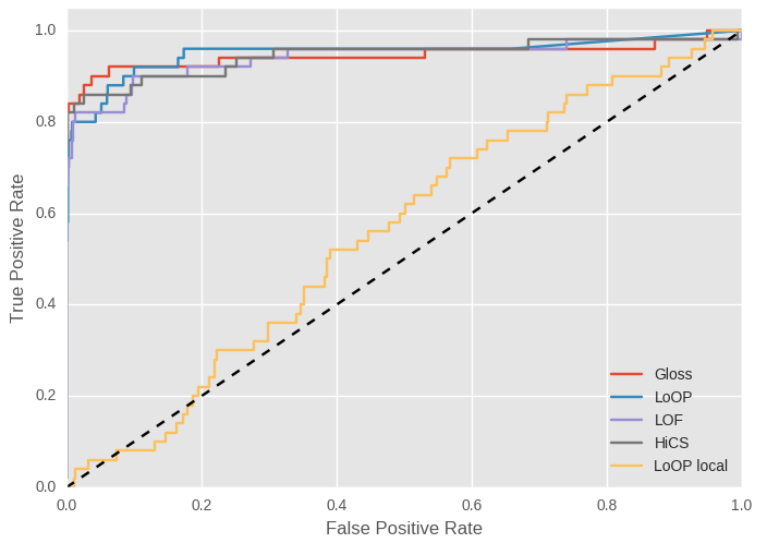
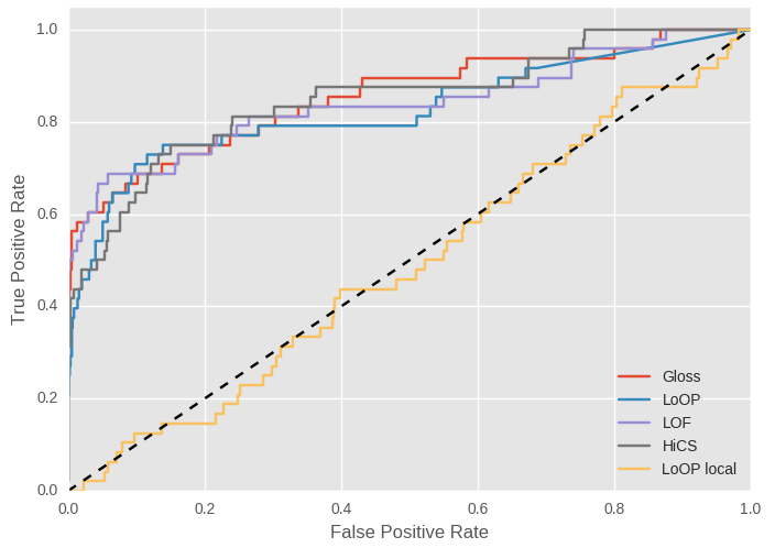
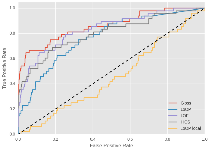
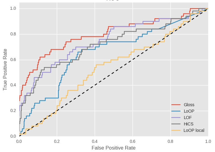
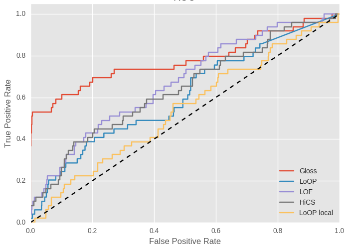
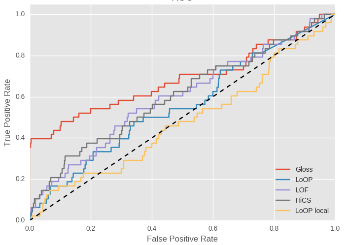
Results Figure 2 shows ROC curves for all algorithms per dimensionality, using clusters and drawn from . Table I presents the obtained AUC scores and runtimes averaged over all runs per dimensionality. It can be observed from Table I that the purely local subspace analysis done by Local LoOP completely fails to identify the ‘hidden’ outliers, whereas HiCS and the global outlier detection methods fail when the number of dimensions increases. Gloss, on the other hand, is able to detect most outliers even when the dimensionality increases all the way up to . From the ROC curves in Figure 2 it can be observed that Gloss tends to find many more outliers at very low false positive rates, while other algorithms only manage to catch up once the false positives rate increases substantially. From the results per individual parameter setting (not included here but available on GitHub), we can see that a higher makes it easier for all algorithms to detect the outliers. This makes sense, since the clusters become more separated and therefore the impact of the local deviation on the global space will be higher. The number of clusters in the data does not seem to be of substantial importance.
| AUC | Runtime | |||||||||
|---|---|---|---|---|---|---|---|---|---|---|
| d | Gloss | HiCS | LOF | LoOP | L.LoOP | Gloss | HiCS | LOF | LoOP | L.LoOP |
| 10 | 0.955 | 0.964 | 0.959 | 0.956 | 0.547 | 2.28 | 3.21 | 0.05 | 0.44 | 1.93 |
| 20 | 0.951 | 0.937 | 0.943 | 0.940 | 0.525 | 4.04 | 3.57 | 0.10 | 0.46 | 3.49 |
| 50 | 0.940 | 0.923 | 0.923 | 0.900 | 0.512 | 12.24 | 9.32 | 0.20 | 0.68 | 8.74 |
| 100 | 0.931 | 0.897 | 0.899 | 0.849 | 0.536 | 30.03 | 41.16 | 0.39 | 0.93 | 17.70 |
| 200 | 0.916 | 0.848 | 0.869 | 0.799 | 0.519 | 79.43 | 91.51 | 0.64 | 1.70 | 38.66 |
| 400 | 0.901 | 0.813 | 0.844 | 0.734 | 0.477 | 225.95 | 232.89 | 1.25 | 2.49 | 57.62 |
| #D | HiCS | Gloss | LOF | LoOP | Local LoOP |
|---|---|---|---|---|---|
| 10 | 3.21 | 2.28 | 0.05 | 0.44 | 1.93 |
| 20 | 3.57 | 4.04 | 0.10 | 0.46 | 3.49 |
| 50 | 9.32 | 12.24 | 0.20 | 0.68 | 8.74 |
| 100 | 41.16 | 30.03 | 0.39 | 0.93 | 17.70 |
| 200 | 336.55 | 79.43 | 0.64 | 1.70 | 38.66 |
| 400 | 2419.99 | 225.95 | 1.25 | 2.49 | 57.62 |
VI-B Benchmark Data with Implanted Outliers
Setup We next compare Gloss to its competitors using a large set of well-known benchmark data from the UCI machine learning repository [20]: Ann Thyroid, Arrhythmia, Glass, Diabetes, Ionosphere, Pen Digits 16, Segments, Ailerons, Pol, Waveform 5000, Mfeat Fourier and Optdigits.
Previous papers usually considered the minority class as ‘outlier class’ for purposes of evaluation, but this clearly would not demonstrate the strengths of our approach: we assume the data to be a mixture of components (i.e., classes), and we search for outliers within those classes. We therefore use the UCI datasets as examples of realistic data and implant artificial outliers. That is, we pick a random sample of of the data points and transform each such data point to an outlier by replacing a randomly picked subspace with the values of a data point from a different class (the size of each subspace was chosen uniformly from ). Note that the datasets most likely already contain ‘natural’ outliers, which makes the task at hand even more difficult.
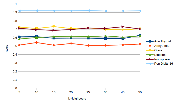
Results Figure 3 shows the effect of the neighbourhood size on the performance of Gloss. It can be seen that the method is very robust with respect to this setting. As is considered to be a “good” choice in literature for LoOP and related local outlier detection methods, we chose this as the default for all other experiments and methods.
Table III presents average AUC scores and running times over ten runs per dataset, together with basic dataset properties, for all competing methods. Gloss clearly outperforms its competitors for most datasets when it comes to AUC and is about as fast as HiCS. From this we can conclude that it is beneficial to use Gloss when the data consists of multiple components and outliers may be hidden as a result of that.
| AUC | Runtime | |||||||||||
|---|---|---|---|---|---|---|---|---|---|---|---|---|
| Dataset | Gloss | HiCS | LOF | LoOP | L.LoOP | Gloss | HiCS | LOF | LoOP | L.LoOP | ||
| Ann Thyroid | 3772 | 30 | 0.608 | 0.565 | 0.595 | 0.591 | 0.545 | 115.851 | 34.864 | 0.316 | 1.259 | 20.11 |
| Arrhythmia | 452 | 279 | 0.543 | 0.529 | 0.505 | 0.531 | 0.533 | 327.887 | 1517.813 | 0.134 | 0.471 | 22.447 |
| Glass | 214 | 9 | 0.733 | 0.675 | 0.708 | 0.709 | 0.546 | 20.535 | 14.489 | 0.004 | 0.048 | 0.326 |
| Diabetes | 768 | 8 | 0.615 | 0.586 | 0.602 | 0.615 | 0.507 | 25.123 | 10.185 | 0.012 | 0.158 | 0.95 |
| Ionosphere | 351 | 34 | 0.69 | 0.608 | 0.636 | 0.61 | 0.573 | 17.65 | 13.171 | 0.015 | 0.098 | 2.074 |
| Pen Digits 16 | 10692 | 16 | 0.92 | 0.86 | 0.915 | 0.91 | 0.497 | 236.956 | 53.43 | 1.555 | 3.07 | 28.759 |
| Segments | 2310 | 20 | 0.815 | 0.8 | 0.765 | 0.797 | 0.745 | 61.859 | 15.292 | 0.159 | 0.595 | 7.619 |
| Ailerons | 13750 | 41 | 0.685 | 0.609 | 0.507 | 0.653 | 0.612 | 396.812 | 91.992 | 0.718 | 8.238 | 109.757 |
| Pol | 15000 | 49 | 0.576 | 0.538 | 0.589 | 0.581 | 0.506 | 475.186 | 256.413 | 4.934 | 7.64 | 168.485 |
| Waveform 5000 | 5000 | 41 | 0.568 | 0.568 | 0.58 | 0.568 | 0.53 | 172.144 | 76.546 | 2.618 | 2.767 | 34.851 |
| Mfeat Fourier | 2000 | 77 | 0.627 | 0.543 | 0.594 | 0.567 | 0.512 | 84.378 | 53.707 | 0.797 | 1.232 | 29.244 |
| Optdigits | 5620 | 65 | 0.688 | 0.584 | 0.675 | 0.659 | 0.518 | 209.598 | 117.749 | 4.951 | 4.601 | 73.045 |
| Average | 0.672 | 0.622 | 0.639 | 0.649 | 0.552 | 174.145 | 176.619 | 1.249 | 2.342 | 38.739 | ||
VI-C Benchmark Data with Minority Class as Outliers
Setup We do not expect using the minority class of a dataset as outlier class to demonstrate the strengths of our approach. Nevertheless, we do not want our improved algorithm to perform worse on the regular local outlier detection task either. Hence, we also compare Gloss to its competitors using the same benchmark datasets but with outliers defined by the more usual procedure of using the minority class as ‘outlier class’. Apart from that, we use the same setup and parameters as in Section VI-B.
Results Table IV presents the average AUC scores obtained over ten runs per dataset. The results show that Gloss performs pretty much on par with the state-of-the-art, demonstrating that our proposed method is capable of detecting ‘regular’ outliers as well as the ones that Gloss identifies but other methods miss (see previous subsections).
| Dataset | Gloss | HiCS | LOF | LoOP | L.LoOP |
|---|---|---|---|---|---|
| Ann Thyroid | 0.759 | 0.581 | 0.727 | 0.779 | 0.889 |
| Arrhythmia | 0.581 | 0.646 | 0.48 | 0.617 | 0.582 |
| Glass | 0.771 | 0.818 | 0.815 | 0.744 | 0.621 |
| Diabetes | 0.575 | 0.512 | 0.495 | 0.566 | 0.508 |
| Ionosphere | 0.886 | 0.921 | 0.881 | 0.881 | 0.733 |
| Pen Digits 16 | 0.473 | 0.522 | 0.461 | 0.465 | 0.524 |
| Segments | 0.522 | 0.493 | 0.512 | 0.52 | 0.530 |
| Ailerons | 0.839 | 0.977 | 0.185 | 0.634 | 0.987 |
| Pol | 0.445 | 0.461 | 0.439 | 0.434 | 0.467 |
| Waveform 5000 | 0.503 | 0.496 | 0.498 | 0.5 | 0.512 |
| Mfeat Fourier | 0.442 | 0.518 | 0.487 | 0.439 | 0.5 |
| Optdigits | 0.519 | 0.57 | 0.538 | 0.545 | 0.483 |
| Average | 0.61 | 0.626 | 0.543 | 0.594 | 0.611 |
VI-D Case Study: Outlier Detection for Quality Control
The last series of experiments of this section are performed on a proprietary dataset made available by the BMW Group at plant Regensburg. This dataset was one the motivations for this work: the data is high-dimensional and a mixture of different, unknown components. Moreover, it is essential for BMW to be able to identify any outliers in the data, as this directly influences their car manufacturing process.
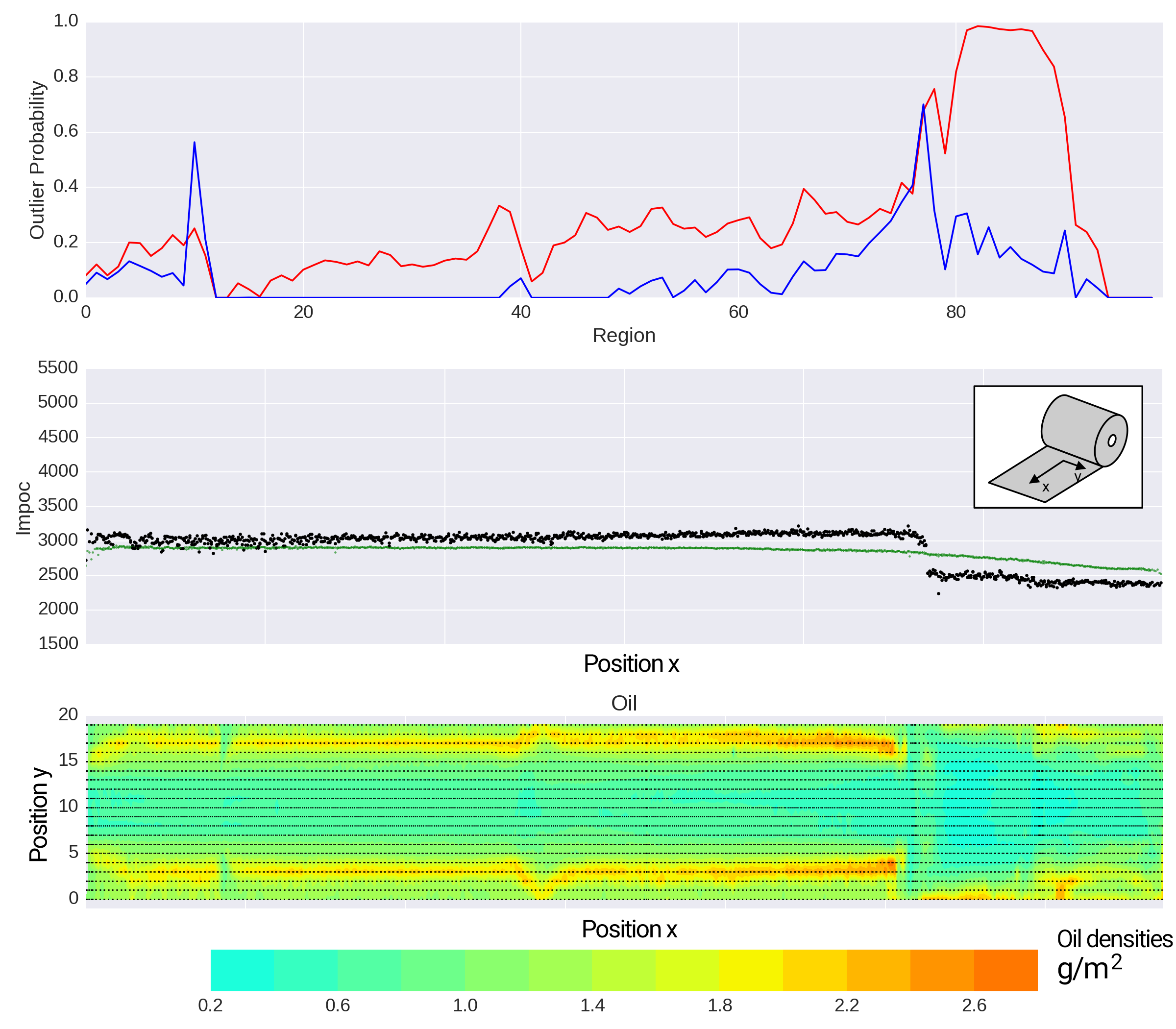
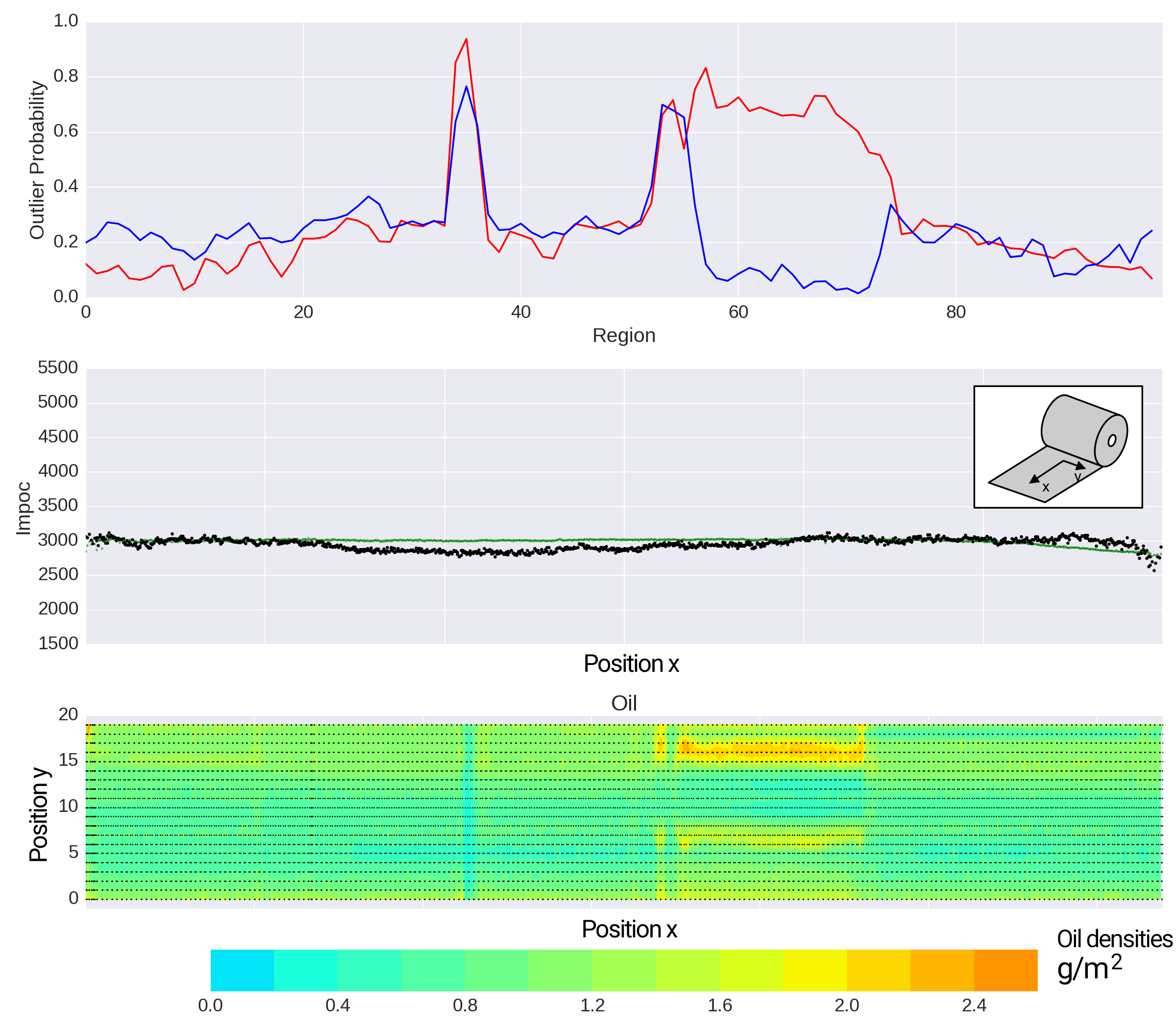
The data concerns steel coils, which is the raw material used as input at the stamping plant (also called ‘press shop’). Before entering the stamping process, each coil—of 2–3 km long—is unrolled and cut into shorter pieces. During this process, a large number of measurements is made. We aim to use these measurements to detect steel coils that strongly deviate from a typical coil in some specific region. A complicating factor is that the data contains measurements for different types of steel from different suppliers, but this important information is not available in the data. Hence, we are dealing with mixed data and we are thus facing exactly the problem formalised as Problem 1, for which we proposed Gloss as solution.
Setup The dataset, containing all measurements done from December 2014 to December 2015, consists of data points and has dimensions, grouped into -dimensional subspaces using the spatial aspects of the data. Each data point represents a coil having segments (in length) and tracks (in width). The most important measurements [21], and the ones we use, are Impoc, quantifying magnetic properties of the steel, and Oil levels, quantifying the amount of oil on the coil. Each subspace consists of Impoc and Oil level values averaged over a segment of size of the length of the coil; the subspaces are consecutive, overlapping segments covering the entire coil.
We compare Gloss to LoOP using all global features and to Local LoOP ran on each of the individual segments/subspaces. Other algorithms are not included in the evaluation because of the high dimensionality of the data; runtimes would be unreasonably long.
Results As expected, LoOP is unable to detect local outliers: it does not take advantage of the spatial information and cannot deal with the very large number () of dimensions. The results obtained by Gloss and our Local LoOP variant are generally similar, but are substantially—and importantly—different for some of the steel coils, as we will show in detail shortly. Moreover, Local LoOP is slower than Gloss, since the neighbourhood of a coil needs to be computed for each individual subspace, whereas Gloss only needs to compute a global neighbourhood once.
We now zoom in on the coils recorded in March , a representative month. By focusing on data from a specific month, we simulate the setting in which the stamping plant operator will inspect the results in the future; Gloss is currently being implemented in the production environment at BMW. Given that deviations in the steel coils directly influence the manufacturing process, this is expected to improve the stability of the process and the quality of the products.
When comparing the outlier rankings obtained with Gloss and Local LoOP for this particular month, we observe that many top outliers appear in high positions in both rankings. However, 1) some coils are ranked very differently by the two approaches and 2) Gloss ranks some coils as outliers that Local LoOP does not. Two such coils are depicted in Figure 4 and 5, showing both the outlier probabilities computed by both methods, and the Impoc and Oil level measurements. While Gloss ranks this coil th and th respectively, Local LoOP ranks them th and th. Clearly an operator would inspect this coil, labelled , if Gloss were used to rank the coils, but not if Local LoOP would have been used. We asked a domain expert to inspect the measurements and outlier probabilities of this coil and others. He reported back to us that the probabilities computed using Gloss more accurately reflect the extend to which the coils are outliers.
Next, to further validate the rankings provided by our method, a domain expert of BMW was shown two top-10 outlier coil rankings, one obtained by Gloss and one by Local LoOP (without duplicates; a coil was left out from a ranking if it was ranked higher by the other method). Of course, the test was blind, i.e., the domain expert did not know which method generated which ranking. For each coil in either top-10, the domain expert was shown the plots as in Figures 4 and 5, but only with the outlier probabilities for the corresponding method. Given the two rankings and plots, the domain expert was asked to rank the (unique) coils according to the perceived degree of outlierness from the domain perspective. Table V shows the labels for the coils in the top-10 rankings of Local LoOP and Gloss, plus the ranking given by the domain expert (using these labels). It is striking that the top four coils selected by the domain expert were all selected by Gloss, with the top ranked coil being the same coil as the top ranked coil identified by Gloss. This confirms that our proposed algorithm is capable of detecting and ranking important outliers that existing algorithms overlook.
| Rank | L.LoOP | Gloss | BMW Expert |
|---|---|---|---|
| 1 | A1 | B1 | B1 |
| 2 | A2 | B2 | B10 |
| 3 | A3 | B3 | B6 |
| 4 | A4 | B4 | B3 |
| 5 | A5 | B5 | A6 |
| 6 | A6 | B6 | A1 |
| 7 | A7 | B7 | B8 |
| 8 | A8 | B8 | A10 |
| 9 | A9 | B9 | A4 |
| 10 | A10 | B10 | B4 |
For the application at our industrial partner, deviations in the measurements often indicate problems with the material and these may cause problems during the manufacturing process. Per year, over coils are processed at this plant, making it infeasible for operators to inspect every single coil. Thus, Gloss will help to narrow this down by providing outlier rankings and probabilities.
VII Conclusions
Motivated by a real-world problem from the automotive industry, we introduced the generic Local Subpace Outlier in Global Neighbourhood problem, and Gloss, an algorithm that addresses this problem. To enable accurate local subspace outlier detection in high-dimensional data that is a mixture of components, Gloss uses neighbourhoods selected in the global data space. The experiments show that Gloss outperforms state-of-the-art algorithms in finding local subspace outliers. Moreover, the experiments show that not only local subspace outliers can be found by Gloss, but Gloss performs on par with the state-of-the-art on the regular outlier detection task. The case study on high-dimensional measurement data from steel coils demonstrates that Gloss is capable at finding relevant local subspace outliers that would otherwise remain undetected, confirming that one should keep an eye on the global perspective even when performing local outlier detection.
References
- [1] V. J. Hodge and J. Austin, “A survey of outlier detection methodologies,” Artificial Intelligence Review, vol. 22, no. 2, pp. 85–126, 2004.
- [2] V. Bamnett and T. Lewis, “Outliers in statistical data,” Journal of the Royal Statistical Society. Series A (General), vol. 141, no. 4, 1994.
- [3] M. M. Breunig, H.-P. Kriegel, R. T. Ng, and J. Sander, “LOF: Identifying Density-Based Local Outliers,” ACM SIGMOD Record, vol. 29, no. 2, pp. 93–104, jun 2000. [Online]. Available: http://portal.acm.org/citation.cfm?doid=335191.335388
- [4] S. Papadimitriou, H. Kitagawa, P. B. Gibbons, and C. Faloutsos, “Loci: Fast outlier detection using the local correlation integral,” Data Engineering, 2003. Proceedings. 19th International Conference on, pp. 315–326, 2003.
- [5] H.-P. Kriegel, P. Kröger, E. Schubert, and A. Zimek, “LoOP: local outlier probabilities,” Proceedings of the 18th ACM conference on Information and knowledge management, pp. 1649–1652, 2009. [Online]. Available: http://doi.acm.org/10.1145/1645953.1646195
- [6] F. Keller, E. Müller, and K. Böhm, “Hics: high contrast subspaces for density-based outlier ranking,” in Data Engineering (ICDE), 2012 IEEE 28th International Conference on. IEEE, 2012, pp. 1037–1048.
- [7] H.-P. Kriegel, P. Kröger, E. Schubert, and A. Zimek, “Outlier detection in axis-parallel subspaces of high dimensional data,” in Advances in Knowledge Discovery and Data Mining. Springer, 2009, pp. 831–838.
- [8] H. Kriegel, P. Kroger, E. Schubert, and A. Zimek, “Outlier detection in arbitrarily oriented subspaces,” in Data Mining (ICDM), 2012 IEEE 12th International Conference on. IEEE, 2012, pp. 379–388.
- [9] A. Loureiro, L. Torgo, and C. Soares, “Outlier detection using clustering methods: a data cleaning application,” in Proceedings of KDNet Symposium on Knowledge-based Systems for the Public Sector. Bonn, Germany, 2004.
- [10] V. Hautamäki, I. Kärkkäinen, and P. Fränti, “Outlier detection using k-nearest neighbour graph.” in ICPR (3), 2004, pp. 430–433.
- [11] S. Upadhyaya and K. Singh, “Classification based outlier detection techniques,” International Journal of Computer Trends and Technology, vol. 3, no. 2, pp. 294–298, 2012.
- [12] K. Choy, “Outlier detection for stationary time series,” Journal of Statistical Planning and Inference, vol. 99, no. 2, pp. 111–127, 2001.
- [13] E. M. Knorr, R. T. Ng, and V. Tucakov, “Distance-based outliers: algorithms and applications,” The VLDB Journal–The International Journal on Very Large Data Bases, vol. 8, no. 3-4, pp. 237–253, 2000.
- [14] D. Pokrajac, A. Lazarevic, and L. J. Latecki, “Incremental Local Outlier Detection for Data Streams,” Computational Intelligence and Data Mining, 2007. CIDM 2007. IEEE Symposium on, no. February, pp. 504–515, 2007.
- [15] F. Chen, C.-T. Lu, and A. P. Boedihardjo, “Gls-sod: a generalized local statistical approach for spatial outlier detection,” in Proceedings of the 16th ACM SIGKDD international conference on Knowledge discovery and data mining. ACM, 2010, pp. 1069–1078.
- [16] X. Liu, C.-T. Lu, and F. Chen, “Spatial outlier detection: Random walk based approaches,” in Proceedings of the 18th SIGSPATIAL International Conference on Advances in Geographic Information Systems. ACM, 2010, pp. 370–379.
- [17] E. Schubert, A. Zimek, and H.-P. Kriegel, “Local outlier detection reconsidered: a generalized view on locality with applications to spatial, video, and network outlier detection,” Data Mining and Knowledge Discovery, vol. 28, no. 1, pp. 190–237, 2014.
- [18] E. Muller, I. Assent, P. Iglesias, Y. Mulle, and K. Bohm, “Outlier ranking via subspace analysis in multiple views of the data,” in Data Mining (ICDM), 2012 IEEE 12th International Conference on. IEEE, 2012, pp. 529–538.
- [19] R. J. G. B. Campello, D. Moulavi, A. Zimek, and J. Sander, “Hierarchical density estimates for data clustering, visualization, and outlier detection,” ACM Trans. Knowl. Discov. Data, vol. 10, no. 1, pp. 5:1–5:51, Jul. 2015. [Online]. Available: http://doi.acm.org/10.1145/2733381
- [20] K. Bache and M. Lichman, “UCI machine learning repository,” http://archive.ics.uci.edu/ml, 2013.
- [21] S. Purr, J. Meinhardt, A. Lipp, A. Werner, M. Ostermair, and B. Glück, “Stamping plant 4.0–basics for the application of data mining methods in manufacturing car body parts,” in Key Engineering Materials, vol. 639. Trans Tech Publ, 2015, pp. 21–30.