Algebraic Multigrid Preconditioners for Multiphase Flow in Porous Media

Abstract

Multiphase flow is a critical process in a wide range of applications, including carbon sequestration, contaminant remediation, and groundwater management. Typically, this process is modeled by a nonlinear system of partial differential equations derived by considering the mass conservation of each phase (e.g., oil, water), along with constitutive laws for the relationship of phase velocity to phase pressure. In this study, we develop and study efficient solution algorithms for solving the algebraic systems of equations derived from a fully coupled and time-implicit treatment of models of multiphase flow. We explore the performance of several preconditioners based on algebraic multigrid (AMG) for solving the linearized problem, including “black-box” AMG applied directly to the system, a new version of constrained pressure residual multigrid (CPR-AMG) preconditioning, and a new preconditioner derived using an approximate Schur complement arising from the block factorization of the Jacobian. We show that the new methods are the most robust with respect to problem character as determined by varying effects of capillary pressures, and we show that the block factorization preconditioner is both efficient and scales optimally with problem size.

1 Introduction

Multiphase flow is a feature of many physical systems and models of it are used in applications such as reservoir simulation, carbon sequestration, ground water management and contaminant transport. Modeling multiphase flow in highly heterogeneous media with complex geometries is difficult, especially when realistic processes such as capillary pressure are included. The system describing multiphase flow consists of nonlinear partial differential equations, constitutive laws and constraints. In this paper, we focus on the iterative solution of linear systems arising in a fully implicit cell-centered finite volume discretization of single component isothermal two-phase flow model with capillary pressure. This fully implicit time-stepping scheme is among the most robust for simulation of subsurface flow. Moreover, it can serve as a basis for modeling more complex processes in which the physical quantities are tightly coupled. This additional complexity could include adding more components, miscibility between components, thermal effects, and phase transitions.

The fully implicit discretization gives rise to a nonlinear system of equations at each time step. We employ a variant of Newton’s method with an exact Jacobian of the discretized equations to solve this system. For the linear system, we use a preconditioned generalized minimal residual (GMRES) method. There is a vast literature on different approaches to precondition the Jacobian system. A very popular approach is to use incomplete LU factorization (ILU) for constructing the preconditioner. Though popular for its general applicability, ILU-based preconditioners are neither effective nor scalable in many cases. Another approach is to consider decoupled preconditioners for the coupled system [6]. This methodology is based on a direct solution of the decoupled pressure system, followed by an iterative solution using ILU for the global system. This formulation was refined in [31], where it was proposed to solve the pressure system iteratively, giving rise to the decoupled implicit pressure explicit saturation (IMPES) preconditioner. The effect of the decoupling is to weaken the coupling between pressure and saturation. Thus, it is often used as a preprocessing step to produce a modified Jacobian system, for which new preconditioners can be developed [10, 30]. With recent development of algebraic multigrid (AMG) algorithms, the pressure block can be solved efficiently using AMG, resulting in the constrained pressure residual multigrid (CPR-AMG) approach. In recent developments, AMG has also been applied to solve the coupled system with some success [10, 30], although developing a general AMG algorithm for these types of problems remains a topic of ongoing research [21]. Since the Jacobian matrix has a block structure, one can also consider a block LU decomposition with an approximate Schur complement, which has been successfully applied to other models of fluid dynamics [22, 33]. Besides AMG-based methods, geometric multigrid has also been applied successfully to solve these types of problems [4, 5]. Our focus in this study is on methods based on AMG because of its general applicability.
In this paper, we develop a new block preconditioner designed to respect the coupling inherent in models of multiphase flow, and we report our experience with the performance and scalability of four different preconditioning strategies: (1) a direct algebraic multigrid (AMG) preconditioner for the global system, (2) two-stage CPR-AMG method with correction for the pressure block, also known as the combinative two-stage approach, (3) CPR-AMG with corrections for both the pressure and saturation blocks, known as the two-stage additive approach, and (4) the block factorization (BF) preconditioner. An outline of the paper is as follows. In section 2, we present the mathematical formulation for two-phase flow in porous media and discretization schemes. In section 3, we describe the solution algorithms for the linearized system. Numerical results for the algorithms are presented in section 4. We conclude with some remarks and discussion of future research directions in section 5.

2 Problem Statement

We consider isothermal, immiscible two-phase flow through a porous medium. For example, often in reservoir simulation, one phase is oil (the nonwetting phase) and the other is pure water (wetting phase); alternatively, in groundwater management, one may consider a system of contaminated water that infiltrates a domain saturated with air.
Conservation of mass of each of the phases leads to the following coupled PDEs:

(1) $$\phi\dfrac{\partial(\rho_{w}s_{w})}{\partial t}+\nabla\cdot(\rho_{w}\mathbf{v}_{w})=q_{w}$$

(2) $$\phi\dfrac{\partial(\rho_{n}S_{n})}{\partial t}+\nabla\cdot(\rho_{n}\mathbf{v}_{n})=q_{n}$$

in which $S_{w},S_{n}$ are the saturation, $\rho_{w},\rho_{n}$ are the densities, $q_{w},q_{n}$ are the source terms of the wetting and non-wetting phases respectively, and $\phi$ is the porosity of the medium. We assume a common extension of Darcy’s law to multiphase flow and express the phase velocities $\mathbf{v}_{w},\mathbf{v}_{n}$ as

(3) $$\mathbf{v}_{\alpha}=-\dfrac{k_{r\alpha}\mathbf{K}}{\mu_{\alpha}}(\nabla P_{\alpha}-\rho_{\alpha}g\nabla D),\hskip 14.22636pt\alpha=w,n.$$

Here, $\mathbf{K}$ is the absolute permeability tensor. The terms $k_{r\alpha},\mu_{\alpha},P_{\alpha}$ are the relative permeability, viscosity, and pressure of phase $\alpha$ respectively, $g$ is the gravitational constant, and $D$ is the depth. We also define the phase mobility $\lambda_{\alpha}=k_{r\alpha}/\mu_{\alpha}$. To close the system, we also have the following constitutive law and constraint

(4) $$Pc(S_{w})=P_{n}-P_{w}$$

(5) $$S_{w}+S_{n}=1$$

From equations Eqs. 1 and 2, one can derive separate equations for pressure and saturation. The pressure equation is elliptic or parabolic (diffusion); the saturation equation is hyperbolic or convection-dominated. The pressure equation is solved implicitly, and depending on the time discretization strategies applied to the saturation equation, several methods have been developed. In the case where the saturation equation is discretized using an explicit method (e.g., forward Euler), it is referred as IMPES (implicit pressure explicit saturation)[3]; for an implicit time discretization of the saturation equation, the method is known as the sequential approach, which was first applied to the black-oil model by Watts in 1985 [32].
The appeal of these methods lies in the sequential decoupling between pressure and saturation variables. Each equation can be solved separately. In addition, knowing the characteristics of each equation facilitates the design of efficient preconditioners, which is critical to achieving high performance. Both of these methods have been successfully applied to many problems where the fully implicit method is difficult to implement or shown to be too costly. However, the solution obtained from these approaches may lose accuracy if pressure and saturation are strongly dependent, or if capillary pressure changes very quickly. The lack of accuracy of these methods can be even more pronounced if more complex processes such as miscibility, thermal, and phase transitions are included in the model. For a more complete summary of the advantages and disadvantages of these approaches, we refer to [19].
Substitution of Eqs. 3 and 4 into Eqs. 1 and 2 and using the constraint Eq. 5 yields a system of two equations and two unknowns. Using one popular choice of primary variables, the pressure in the wetting phase and saturation in the nonwetting phase, $\mathbf{u}=(P_{w},S_{n})$, we obtain

(6) $$- \dfrac{\partial(\phi\rho_{w}S_{n})}{\partial t}-\nabla\cdot\Big{(}\rho_{w}\dfrac{k_{rw}(S_{n})}{\mu_{w}}\mathbf{K}(\nabla P_{w}-\rho_{w}g\nabla D)\Big{)}=q_{w}$$

(7) $$\dfrac{\partial(\phi\rho_{n}S_{n})}{\partial t}-\nabla\cdot\Big{(}\rho_{n}\dfrac{k_{rn}(S_{n})}{\mu_{n}}\mathbf{K}(\nabla(P_{w}+P_{c}(S_{n}))-\rho_{n}g\nabla D)\Big{)}=q_{n}.$$

In this paper, we consider solving the coupled system consisting of Eqs. 6 and 7 fully implicitly. We use a cell-centered finite volume method for spatial discretization and the backward Euler method for time discretization, similar to an approach defined in [13]. This will serve as a base model for adding more complexity in the future. The finite volume method described below is known for its mass conservation property. In addition, it can deal with the case of discontinuous permeability coefficients, and it is relatively straightforward to implement. Under appropriate assumptions, this method also falls into the mixed finite element framework [23, 26]. For simplicity, we consider a uniform partitioning of the domain $\mathbf{\Omega}$ into equal sized cells $C_{i}$, i.e., $\mathbf{\Omega}=\bigcup\limits_{i=1}C_{i}$. Let $\gamma_{ij}$ denote the area of the face between cells $C_{i}$ and $C_{j}$. For each cell $C_{i}$, integration of the mass conservation equations and the divergence theorem gives

(8) $$\dfrac{\partial}{\partial t}\int_{C_{i}}\xi_{\alpha}+\sum_{j\in\eta_{i}}\int_{\gamma_{ij}}\psi_{\alpha}\cdot\mathbf{n}=\int_{C_{i}}q_{\alpha}$$

where the storage $\xi_{\alpha}=\phi\rho_{\alpha}S_{\alpha}$ and the flux $\psi_{\alpha}=\rho_{\alpha}\mathbf{v}_{\alpha}$ terms are approximated using the mid-point rule which is second-order accurate:

(9) $$\bar{\xi}_{\alpha}=\dfrac{1}{V_{C_{i}}}\int_{C_{i}}\xi_{\alpha},\hskip 8.53581ptQ_{\alpha}=\dfrac{1}{V_{C_{i}}}\int_{C_{i}}q_{\alpha}.$$

The surface integrals are discretized using two-point flux approximation (TPFA); dropping the phase subscript, this gives

(10) $$\int_{\gamma_{ij}}\psi\cdot\mathbf{n}=-\gamma_{ij}\Big{(}\rho\dfrac{k_{r}}{\mu}\mathbf{K}\Big{)}_{ij+1/2}\big{(}\omega_{i}-\omega_{j}\big{)}\,,$$

(11) $$\omega_{i}=\dfrac{P_{i}-\rho_{ij+1/2}\;gD_{i}}{\Delta x_{ij+1/2}}\;.$$

The index $ij+1/2$ signifies an appropriate averaging of properties at the interface between cell $i$ and $j$. The coefficients $(\rho k_{r}/\mu)_{ij+1/2}$ are approximated by upwinding based on the direction of the velocity field, i.e.,

(12) $$\Big{(}\rho\dfrac{k_{r}}{\mu}\Big{)}_{ij+1/2}=\begin{cases}\Big{(}\rho\dfrac{k_{r}}{\mu}\Big{)}_{i}\;,\hskip 14.22636pt\text{if }\mathbf{v}\cdot\mathbf{n}>0\\ \Big{(}\rho\dfrac{k_{r}}{\mu}\Big{)}_{j}\;,\hskip 14.22636pt\text{otherwise}\end{cases}$$

and the absolute permeability tensor on the faces are computed using harmonic averaging,

(13) $$\mathbf{K}_{ij}=(\Delta x_{i}+\Delta x_{j})\Big{(}\dfrac{\mathbb{K}_{i}\mathbb{K}_{j}}{\Delta x_{i}\mathbb{K}_{j}+\Delta x_{j}\mathbb{K}_{i}}\Big{)}.$$

Discretization in time using the backward Euler method gives a fully discrete system of nonlinear equations,

(14) $$(\bar{\xi})_{i}^{n+1}-(\bar{\xi})_{i}^{n}= -\dfrac{\bigtriangleup t}{V_{C_{i}}}\sum_{j\in\eta_{i}}\gamma_{ij}\left(\rho\dfrac{k_{r}}{\mu}\mathbb{K}\right)_{ij+1/2}^{n+1}\Big{(}\omega_{i}^{n+1}-\omega_{j}^{n+1}\Big{)}-Q^{n+1}.$$

3 Solution Algorithms

The system of nonlinear equations (14) can be written generically as $F(u)=0$ where $F:\mathbb{R}^{n}\rightarrow\mathbb{R}^{n}$. We solve the system using Newton’s method, which requires solution of a linear system at each iteration $k$:

(15) $$\dfrac{\partial F}{\partial u}\Big{|}_{u=u_{k}}(u_{k+1}-u_{k})=-F(u_{k}).$$

In our case, the solution vector $u$ consists of all the pressure and saturation unknowns at all the cell centers. The Jacobian system resulting from the derivative $\partial F/\partial u$ is often very difficult to solve using iterative methods, and preconditioning is critical for rapid convergence of Krylov subspace methods such as GMRES [28]. Next, we discuss the linear system arising from the Newton’s method and give a detailed description of the solution algorithms we will use to solve this system.

3.1 Linear System

For the set of primary variables $u=(P_{w},S_{n})$, assuming unknowns corresponding to physical variables are grouped together and unknowns associated with nodal points in the domain are ordered lexicographically, each nonlinear Newton iteration entails the solution of a discrete version of a block linear system of the form

(16) $$\begin{pmatrix}-\nabla\cdot(\lambda_{w}K\nabla)&-\dfrac{\phi}{\partial t}-\nabla\cdot(\mathbf{v}_{w})\\ -\nabla\cdot(\lambda_{n}K\nabla)&\dfrac{\phi}{\partial t}+\nabla\cdot(\mathbf{v}_{n})+\nabla\cdot(\lambda_{n}P_{c}^{\prime}K\nabla)\end{pmatrix}\begin{pmatrix}\delta P_{w}\\ \delta S_{n}\end{pmatrix}=-\begin{pmatrix}q_{w}\\ q_{n}\end{pmatrix}$$

in which

(17) $$\mathbf{v}_{w}=-\lambda_{w}^{\prime}K\nabla\tilde{P}_{w}$$

(18) $$\mathbf{v}_{n}=-\lambda_{n}^{\prime}K\nabla\tilde{P}_{n}+\lambda_{n}K\nabla(P_{c}^{\prime})\;.$$

All the coefficients in equation (16) are evaluated at the linearization point $\tilde{P}_{w},\tilde{S}_{n}$. In a more concise form, the Jacobian matrix of the system has $2\times 2$ block structure

(19) $$J=\begin{pmatrix}A_{pp}&A_{ps}\\ A_{sp}&A_{ss}\end{pmatrix},$$

and the linear system is $Jc=q$. The characteristics of the matrix have been discussed in numerous papers [5, 13, 17, 30]. We summarize important characteristics of the operators here:

• $J$ is nonsymmetric and indefinite

• The block $A_{pp}$ has the structure of a discrete purely elliptic problem for pressure.

• The coupling block $A_{ps}$ has the structure of a discrete first-order hyperbolic problem in the non-wetting phase saturation.

• The coupling block $A_{sp}$ has the structure of a discrete convection-free parabolic problem in the wetting phase pressure.

• The block $A_{ss}$ has the structure of a discrete parabolic (convection-diffusion) problem for saturation when capillary pressure is a non-constant function of the saturation. When capillary pressure is zero or a constant, there is no diffusion term and the block has the form of a hyperbolic problem.

• Under mild conditions, i.e. modest time-step size, the blocks $A_{pp},A_{ps},A_{ss}$ are diagonally dominant.

In this paper, we present some numerical results that show how different models of capillary pressure affect the algebraic properties of the (2,2)-block $A_{ss}$ in particular and the global system in general, which consequently determines the success of AMG solution algorithms. Our emphasis is on the development and use of preconditioning operators denoted $M\approx J$, for the purpose of solving preconditioned systems

(20) $$JM^{-1}\hat{c}=q,\quad c=M^{-1}\hat{c}.$$

3.2 Algebraic Multigrid

Multigrid is a highly efficient and scalable method available for solving large sparse linear systems [34]. Geometric multigrid uses a hierarchy of nested grids, whose construction depends on the geometry of the problem and a priori knowledge of the grids. AMG methods such as those developed in [29] have the advantage of not requiring an explicit hierarchy of nested grids. AMG constructs coarse grids based on the matrix values only, which makes it suitable for solving a wide range of problems on complicated domains and unstructured grids. Despite its successful application to scalar problems, using AMG for coupled systems is still relatively limited. Some attempts to use AMG to solve fully coupled systems encountered in modeling multiphase flow for reservoir simulation include [10, 30]. In this work, we use BoomerAMG [16], part of the Hypre package [14, 15], as a black-box AMG solver. We note that in order to use BoomerAMG for the coupled system in our case, the Jacobian matrix needs to be ordered by grid points, i.e.

(21) $$J=\begin{pmatrix}A_{11}&\ldots&A_{1N}\\ \vdots&\ddots&\ldots\\ A_{N1}&\ldots&A_{NN}\end{pmatrix}$$

in which $N$ is the number of grid points, and $A_{ij}$ are $2\times 2$ matrices representing the couplings between pressure and saturation at points $i$ and $j$. This is called the “point” method in [30].

3.3 Two-stage Preconditioning with AMG

Unlike AMG, which has not been popular in reservoir simulation until recently, two-stage preconditioners are widely used [17]. This idea was developed and first appeared in the context of multiphase flow modeling in the work of Wallis [31]. Following [13], we refer to this method as the constrained pressure residual (CPR) approach. There are many variants of two-stage preconditioners. We discuss two algorithms here: the two-stage combinative preconditioner - CPR-AMG(1), and the two-stage additive preconditioner - CPR-AMG(2) [2].
Algorithm 1. Two-stage Combinative - CPR-AMG(1)

1. At each iteration $k$ let the residual be $r_{k}$.

2. Solve $u_{k+1/2}=P_{1}^{-1}r_{k}$.

3. Update the residual $r_{k+1/2}=r_{k}-Au_{k+1/2}$.

4. Solve for the pressure correction $A_{pp}\delta_{p}=R_{p}r_{k+1/2}$

5. Update the solution $u_{k+1}=u_{k+1/2}+R_{p}^{T}\delta_{p}$

Algorithm 2. Two-stage Additive - CPR-AMG(2)

1. At each iteration $k$ let the residual be $r_{k}$.

2. Solve $u_{k+1/2}=P_{1}^{-1}r_{k}$.

3. Update the residual $r_{k+1/2}=r_{k}-Au_{k+1/2}$.

4. Solve for the pressure correction $A_{pp}\delta_{p}=R_{p}r_{k+1/2}$

5. Solve for the saturation correction $A_{ss}\delta_{s}=R_{s}r_{k+1/2}$

6. Update the solution $u_{k+1}=u_{k+1/2}+R_{p}^{T}\delta_{p}+R_{s}^{T}\delta_{s}$

The matrices $R_{p},R_{s}$ denote the restriction of the global unknown vector to those associated with pressure and saturation respectively. That is, $R_{p}\in\mathbb{R}^{n\times 2n}$ and for $u=\begin{pmatrix}p\\ s\end{pmatrix}$

(22) $$R_{p}u=p,\hskip 14.22636pt R_{p}^{T}u=\begin{pmatrix}p\\ 0\end{pmatrix};\hskip 31.29802ptR_{s}u=s\hskip 14.22636ptR_{s}^{T}u=\begin{pmatrix}0\\ s\end{pmatrix}$$

Then, in matrix form, the action of the two-stage preconditioners can be expressed as

(23) $$u=M_{comb}^{-1}r=(I-R_{p}^{T}A_{pp}^{-1}R_{p}(A-P_{1}))P_{1}^{-1}r$$

(24) $$u=M_{add}^{-1}r=(I-(R_{p}^{T}A_{pp}^{-1}R_{p}+R_{s}^{T}A_{ss}^{-1}R_{s})(A-P_{1}))P_{1}^{-1}r$$

For the preconditioner $P_{1}$ in step 2 of both algorithms, we use the incomplete factorization with no fill ILU(0) method. For the correction solve, we apply AMG with one V-cycle iteration. The combinative approach with AMG was presented in [18, 20]. However, this method does not work well in the presence of fast changing capillary pressure. We confirm this observation in the next section. To deal with fast changing capillary pressure, we employ an additive CPR-AMG approach, which involves one more AMG solve for the correction of the saturation block. The intuition is that when the absolute value of the derivative of capillary pressure $|dP_{c}/dS_{w}|$ is large, the block $A_{ss}$ becomes diffusion dominated, and AMG can handle it efficiently.

3.4 Block Factorization Preconditioners

Consider the following decomposition of the Jacobian,

$$J=\begin{pmatrix}A_{pp}&A_{ps}\\ A_{sp}&A_{ss}\end{pmatrix}=\begin{pmatrix}I&A_{ps}A_{ss}^{-1}\\ 0&I\end{pmatrix}\begin{pmatrix}S&0\\ 0&A_{ss}\end{pmatrix}\begin{pmatrix}I&0\\ A_{ss}^{-1}A_{sp}&I\end{pmatrix},$$

where $S$ is the Schur complement

(25) $$S=A_{pp}-A_{ps}A_{ss}^{-1}A_{sp}.$$

We could choose

(26) $$M=\begin{pmatrix}I&A_{ps}A_{ss}^{-1}\\ 0&I\end{pmatrix}\begin{pmatrix}S&0\\ 0&A_{ss}\end{pmatrix}=\begin{pmatrix}S&A_{ps}\\ 0&A_{ss}\end{pmatrix}$$

as an upper-triangular block preconditioner; this incorporates the effects of the coupling block $A_{ps}$, which contains the time derivative and gravity terms (16). We use an approximation of the Schur complement in which $A_{ss}$ is replaced by its diagonal values:

(27) $$\tilde{S}=A_{pp}-A_{ps}\operatorname{diag}{(A_{ss})}^{-1}A_{pp}.$$

The purpose of this is to keep the Schur complement sparse so that the action of its inverse can be applied efficiently. This idea is the basis of the SIMPLE method used in other models of fluid dynamics [22]. A similar approach has also been applied to problems in single phase flow coupled with geomechanics in [33].
Algorithm 3. Block factorization preconditioner

1. At each iteration $k$ let the residual be $r_{k}$.

2. Solve for the saturation $A_{ss}s_{k+1}=R_{s}r_{k}$ using AMG.

3. Compute the residual for pressure $r=R_{p}r_{k}-A_{ps}s_{k+1}$.

4. Solve for the pressure $\tilde{S}p_{k+1}=r$ using AMG.

An important advantage of this algorithm is that it does not rely on an ILU factorization. In matrix form,

(28) $$M_{bf}^{-1}=\begin{pmatrix}\tilde{S}^{-1}&-\tilde{S}^{-1}A_{ps}A_{ss}^{-1}\\ 0&A_{ss}^{-1}\end{pmatrix}\;.$$

4 Numerical Results

In this section, we perform numerical experiments for the four aforementioned preconditioners. All of them are implemented in Amanzi, a parallel open-source multi-physics C++ code developed as a part of the ASCEM project [1]. Although Amanzi was first designed for simulation of subsurface flow and reactive transport, its modular framework and concept of process kernels [11] allow new physics to be added relatively easily for other applications. The two-phase flow simulator employed in this work is one such example. Amanzi works on a variety of platforms, from laptops to supercomputers. It also leverages several popular packages for mesh infrastructure and solvers through a unified input file. Here, all of our experiments use a classical AMG solver through BoomerAMG in Hypre. The ILU(0) method is from Euclid, also a part of Hypre. GMRES is provided within Amanzi. For simplicity, we employ structured Cartesian grids for the test cases, but we can also use unstructured K-orthogonal grids. This section has three parts. In the first part, we show the results for a two-dimensional oil-water model problem. Although the problem is small, it is difficult to solve due to the heterogeneity of the permeability field. In the second part, we report the results for a three-dimensional example. In the last part, we examine the scalability of the three preconditioning strategies. Unless specified otherwise, we use the benchmark problem SPE10 [8] for permeability data and porosity.

4.1 Two-dimensional oil-water problem

The domain is a rectangle with dimensions $762\times 15.24$ meters. The mesh is $100\times 20$, which means that the problem is truly two-dimensional in the $xz$ plane. We inject pure water into the domain through the boundary at the lower left corner, and oil and water exit the domain through the top right corner. These correspond to the $S_{w}=1.0,\hskip 2.84526pt\lambda_{w}\nabla P_{w}\cdot\mathbf{n}=-50\hskip 5.69054ptm^{3}/day$ at the inlet, and $S_{w}=0.2,\hskip 2.84526ptP_{w}=0$ at the outlet. The simulation is run for 200 days with time step $\Delta t=20\text{ days}$.
For capillary pressure models, we employ a simple linear model and the Brooks-Corey [7] model:

(29) $$\text{Linear model: }P_{c}(S_{w})=P_{0}(1-\bar{S}_{w}),\hskip 14.22636pt\text{Brooks-Corey: }P_{c}(S_{w})=P_{d}\bar{S}_{w}^{-1/\lambda}$$

in which $\bar{S}_{w}$ is the effective saturation, $P_{d}$ is the entry pressure, and $\lambda$ is related to the pore-size distribution. For the Brooks-Corey model, the typical range of $\lambda$ is $\left[0.2,3.0\right]$ [4, 12]. In general, $\lambda$ is greater than 2 for narrow distributions of pore sizes, and $\lambda$ is less than 2 for wide distributions. For example, sandpacks with broader distributions of particle sizes have $\lambda$ ranging from $1.8$ to $3.7$ [24]. The Brooks-Corey capillary pressure curves for various values of $\lambda$ are plotted in Figure 1. Other parameters are listed in Table 2 and example 1 of Table 2.

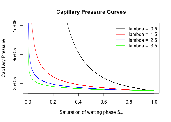
Figure 1: Capillary pressure curves for Brooks-Corey model with entry pressure $P_{d}=10^{5}\hskip 5.69054ptPa$.

For all of the simulations presented here, the convergence tolerance for Newton’s method is $||F(x)||\leq 10^{-6}$, and the linear tolerance for GMRES is $||J\delta u_{k}-F(u_{k})||\leq 10^{-12}||F(u_{k})||$, which is the default in Amanzi. BoomerAMG is used as a preconditioner. The number of V-cycle steps is set to 1. The coarsening strategy is the parallel Cleary-Luby-Jones-Plassman (CLJP) coarsening [9]. The interpolation method is the classical interpolation defined in [25], and the smoother is the forward hybrid Gauss-Seidel / SOR scheme.

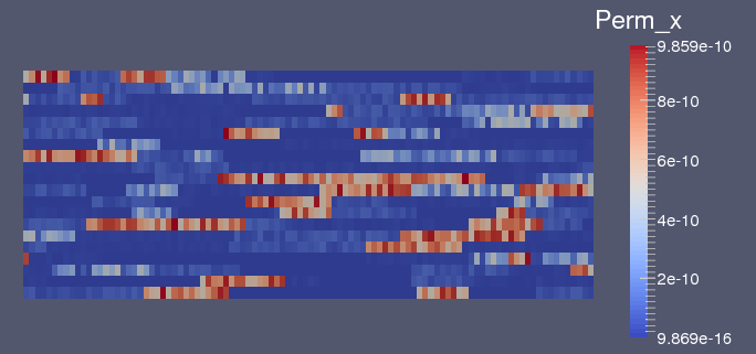
Figure 2: Permeability field obtained from SPE10 model 1 data.
The x-direction is scaled down by $1/20$ for visualization.

Table 1: Input data for the quarter-five spot problem.

Initial wetting phase pressure	$10^{5}$ $Pa$
Initial nonwetting phase saturation	0.8
Residual wetting phase saturation	0.0
Nonwetting phase density	700 $kg/m^{3}$
Wetting phase density	1000 $kg/m^{3}$
Nonwetting phase viscosity	10.0 $cP$
Wetting phase viscosity	1 $cP$
Porosity	0.2

Table 2: Parameters for capillary pressure models

Parameters	Ex 1	Ex 2	Ex 3	Ex 4
Linear entry pressure $P_{0}$	$10^{5}$	$10^{4}$	$10^{3}$	$10^{6}$
Brooks-Corey entry pressure $P_{d}$	$10^{6}$	$10^{5}$	$2\times 10^{4}$	$10^{6}$
Brooks-Corey $\lambda$	2.5	0.8	2.5	0.8

In order to explore the effects of different models for capillary pressure on solver performance, we use the four sets of parameters listed in Table 2. In Example 1, the parameters are chosen such that the $L_{\infty}$ norm of the derivative of capillary pressure $P_{c}^{\prime}$ is large, leading to a diffusion-dominated case (see equation (16)). In Example 2, the parameters are tuned to reduce the $L_{\infty}$ norm of $P_{c}^{\prime}$, leading to an advection-dominated case. Example 3 is a more extreme case of example 2, in which $P_{c}^{\prime}$ is further decreased, leading to a strongly advection-dominated case. We also note the difference between the linear model and the Brooks-Corey model for capillary pressure. The derivative $P_{c}^{\prime}$ for the linear model is a constant value, which means that the character of the problem, i.e. diffusion-dominated or advection-dominated, is the same everywhere for the whole domain. In the Brooks-Corey model, $P_{c}^{\prime}$ depends on the saturation of the wetting phase, and the problem can be diffusion-dominated in one part of the domain, and advection-dominated in another part. This can cause further difficulties for AMG-based solvers, whose optimal performance is sensitive to the characteristics of the problem.

Table 3: Performance of three preconditioning strategies for set of parameters in the diffusion-dominated Example 1.

Methods/Models	Linear				Brooks Corey
	NI	LI	LI/NI	Time	NI	LI	LI/NI	Time
AMG	32	368	11.5	27.2	36	470	13.1	37.24
CPR-AMG(1)	32	3695	115.5	324.15	36	5831	162	567.7
CPR-AMG(2)	32	899	28.1	103.94	36	1102	30.6	134.6
BF	32	524	16.4	33.17	36	599	16.6	46.2

The performance of the three strategies is summarized in Tables 3, 5, and 5. NI denotes the number of nonlinear iterations, LI the number of linear iterations, LI/NI the average number of linear iterations per nonlinear iterations, and Time the total time in seconds of the whole simulation. For the diffusion-dominated problem for which the results are shown in Table 3, AMG is the most efficient method, about 25% more efficient than the block preconditioner in terms of both iteration counts (linear iterations per Newton step) and total run time. Note that for this example, the diffusion terms in the (2,2)-block ($A_{ss}$) are large and the performance of AMG tends to be very strong for problems of this type. For the linear model, the block factorization approach still takes about 8 times fewer linear iterations, and it is about 10 times faster in total run time than CPR-AMG(1). The reason for this discrepancy is that CPR-AMG(1) is a two-stage preconditioner, and it requires an extra global solve using ILU. The block factorization preconditioner does not rely on ILU, which helps improve the run time significantly. CPR-AMG(2) also performs well in this case. Although it requires one more AMG solve per Newton iteration than CPR-AMG(1), it still outperforms CPR-AMG(1) in terms of both the number of linear iterations per Newton step and the total run time. The same conclusion can be made for the Brooks-Corey model.

Table 4: Performance of three preconditioning strategies for set of parameters in the advection-dominated Example 2.

Methods/Models	Linear				Brooks Corey
	NI	LI	LI/NI	Time	NI	LI	LI/NI	Time
AMG	37	2575	69.6	138.8	-	-	-	-
CPR-AMG(1)	37	1919	51.9	175.5	55	4851	88.2	605.7
CPR-AMG(2)	37	1222	33.0	157.1	55	3701	67.3	506.8
BF	37	684	18.5	51.7	55	1633	29.7	131.1

Table 5: Performance of three preconditioning strategies for set of parameters in the strongly advection-dominated Example 3.

Methods/Models	Linear				Brooks Corey
	NI	LI	LI/NI	Time	NI	LI	LI/NI	Time
AMG	-	-	-	-	-	-	-	-
CPR-AMG(1)	43	1079	25.1	122.8	48	2173	45.3	247.6
CPR-AMG(2)	43	1442	35.5	169.8	48	4805	100.1	560.5
BF	43	1002	23.3	69.8	48	1829	38.1	121.8

The results reported in Table 5 reveal the lack of robustness of AMG when applied to the coupled system. In contrast to the diffusion-dominated case, for the linear model of capillary pressure, AMG requires the highest number of linear iterations per Newton step for the advection-dominated case, and it even diverges for the Brooks-Corey model. The block factorization preconditioner still shows good performance, taking about half the number of iterations and running four times faster than the next best method, which is CPR-AMG(2). CPR-AMG(1) is still the least effective method in this case for both capillary pressure models.

For the strongly advection-dominated problem with parameters in example 3, AMG diverges for both the linear and Brooks-Corey capillary pressure models. The performance of CPR-AMG(2) is also affected in this case, trailing that of CPR-AMG(1). CPR-AMG(2) is still more robust than direct application of AMG, however, since unlike AMG, this method still converges. The block factorization preconditioner is again the most effective method, requiring fewer number of iterations and about half the run time of CPR-AMG(1). This suggests that when the diffusion term in the $A_{ss}$ block gets small, the coupling block $A_{ps}$ which has the structure of a discrete first-order hyperbolic problem for the saturation, becomes important and needs to be taken into account.

4.2 Two-dimensional problem with gravity

In this example, we compare the performance of the different strategies for a problem in which gravity plays a dominant role. The domain is a square box of size $20\times 20$ meters. The absolute permeability is a homogeneous field of $100$ millidarcy. Water is injected into the domain through the boundary at the top left corner, and the outlet is at the top right corner. The rate of injection is 5 $m^{3}$/day. For spatial discretization, we use uniform grids of size $20\times 20$, $40\times 40$, $80\times 80$, and $160\times 160$ respectively. The initial conditions are the same as the heterogeneous two-dimensional example above. The time steps are 10, 4, and 1 days, and the final times are 20, 8, and 2 days respectively.

Table 6: Iteration counts for diffusion-dominated case with gravity, time step $dt=10$ days.

Methods/Mesh sizes	$20^{2}$	$40^{2}$	$80^{2}$	$160^{2}$
AMG	7	7	7	7
CPR-AMG(1)	15.1	25.9	49.4	95.2
CPR-AMG(2)	22.0	30.9	38.1	40.7
BF	19.9	21.0	21.1	21.1

Table 7: Iteration counts for advection-dominated case with gravity, time step $dt=4$ days.

Methods/Mesh sizes	$20^{2}$	$40^{2}$	$80^{2}$	$160^{2}$
AMG	-	-	-	17.3
CPR-AMG(1)	17.9	17.8	16.1	25.2
CPR-AMG(2)	30.3	29.8	22.7	30.2
BF	13.0	17.0	21.1	23.9

Table 8: Iteration counts for highly advection-dominated case with gravity, time step $dt=1$ day.

Methods/Mesh sizes	$20^{2}$	$40^{2}$	$80^{2}$	$160^{2}$
AMG	-	-	-	-
CPR-AMG(1)	18.6	19.6	19.7	18.8
CPR-AMG(2)	31.5	34.6	36.6	36.3
BF	13.1	9.3	12.0	16.4

The diffusion-dominated case, shown in Table 8, exhibits the same pattern as in the previous example: the AMG preconditioner is the most efficient method, followed by the block factorization method, CPR-AMG(2), and CPR-AMG(1). AMG and the block factorization method exhibit optimal performance with respect to problem size. The number of iterations for CPR-AMG(2) also seems to reach a plateau as the mesh size is refined. In contrast, the performance of CPR-AMG(1) does not scale well with respect to mesh size for this case, taking about twice the number of iterations for each level of mesh refinement.

The results for the advection-dominated case are shown in Table 8. The AMG method is not robust and only converges for the largest mesh size (for which it takes the fewest iterations). The block factorization preconditioner is highly robust and also appears to require iteration counts tending to a constant as the mesh is refined. The performance of CPR-AMG(2) is consistent except for the $80\times 80$ mesh. Although it requires more iterations than CPR-AMG(1), this method shows promising scaling property, similar to the previous example, since the number of iterations does not grow as the mesh is refined. CPR-AMG(1) performs quite well for this case, but it still exhibits poor scalability as the number of iterations grow quickly between $80\times 80$ and $160\times 160$.

In the strongly advection-dominated case, AMG diverges for all mesh sizes. The new block factorization is the most efficient method in this case, requiring the smallest number of iterations across all mesh sizes. Here, CPR-AMG(1) is more efficient than CPR-AMG(2), requiring about half the number of iterations. Both CPR-AMG(1) and CPR-AMG(2) show good scaling property in this case. The scaling result for the block factorization method is not as clear as in the diffusion and advection dominated cases, but we suspect that the mesh is not fine enough for a consistent pattern to emerge.

Besides varying the mesh size, we also experimented with changing the time step size for a fixed mesh of $80\times 80$ for the same problem. The results are reported in Table 9. The final time for the simulation is 8 days. The results are reported in Table 9.

Table 9: Results for the advection-dominated case with gravity $P_{0}=10^{4}$.
NI/TS is the number of Newton iteration per time step.

Methods/Time steps	$dt$ = 1 day		$dt$ = 2 days		$dt$ = 4 days		$dt$ = 8 days
	NI/TS	LI/NI	NI/TS	LI/NI	NI/TS	LI/NI	NI/TS	LI/NI
CPR-AMG(1)	12.4	16.9	17	15.9	23	16.1	28	19.4
CPR-AMG(2)	12.4	29.0	17	24.0	23	22.7	28	27.2
BF	12.4	16.7	17	19.0	23	21.1	28	23.0

Since AMG does not converge in this experiment, we exclude it from the results. From Table 9, it is clear that as the time step gets larger, Newton’s method takes more iterations to converge. For $dt=$ 8 days, there is only one time step and it is the most difficult case. CPR-AMG(1) number of iterations is not significantly affected by the time step except for the largest time step size of 8 days. Meanwhile, CPR-AMG(2) number of iterations decreases as the time step gets larger, but goes up again at $dt=8$ days. The block factorization method shows consistent increase in the number of iterations for larger time steps. Overall, there is not much of a difference in terms of iteration counts for these three methods, but it is worth noting that the block factorization method is much faster than the others in terms of run time, as it does not require a global ILU solve.

4.3 Behavior of Eigenvalues

It is often possible to obtain insight into the properties of preconditioning operators from the eigenvalues of the preconditioned matrix $JM^{-1}$. In particular, recall a standard analysis of the convergence behavior of GMRES for solving the preconditioned system (20) [27]. Assume the preconditioned matrix is diagonalizable, $JM^{-1}=V\Lambda V^{-1}$, where $\Lambda$ is a diagonal matrix containing the eigenvalues of the preconditioned matrix and the columns of $V$ are the corresponding eigenvectors. If $c_{k}=M^{-1}{\hat{c}}_{k}$ are the iterates obtained at the $k$th step of GMRES iteration, with residual $r_{k}=q-Jc_{k}$, then

(30) $$\frac{\|r_{k}\|_{2}}{\|r_{0}\|_{2}}\leq\|V\|_{2}\,\|V^{-1}\|_{2}\min_{p_{k}(0)=1}\max_{\lambda\in\sigma(JM^{-1})}|p_{k}(\lambda)|,$$

where the minimum in (30) is over all polynomials of degree at most $k$ that have the value $1$ at the origin, $\sigma(JM^{-1})$ is the set of eigenvalues of $JM^{-1}$, and the norm is the vector Euclidian norm. Thus, a good preconditioner tends to produce a preconditioned operator with a compressed spectrum whose entries are not near the origin. In this section, we explore the behavior of the eigenvalues of the preconditioned matrix with an eye toward understanding the effects of features of the discrete problem such as discretization mesh size and qualitative features of the model such as the relative weights of diffusion and advection and the degree of coupling between the components.

Figure 3 gives a representative depiction of the eigenvalues of preconditioned operators for three of the preconditioners considered. These results are for benchmark problems for which performance is considered in section 4.1, the two-dimensional linear oil-water model discretized on a $100\times 20$ grid. The plots on the left side of the figure show eigenvalues for the diffusion-dominated case (for which solution performance is shown in Table 3), and those on the right show eigenvalues for the advection-dominated case (performance in Table 5).

Figure 3: Eigenvalues of preconditioned systems for different strategies, applied to the diffusion-dominated Example 1 (left) and advection-dominated Example 2 (right).

These displays indicate that the spectra for the preconditioned systems for the CPR-AMG(2) and BF preconditioners are bounded away from the origin, whereas for the CPR-AMG(1) preconditioner there are many small eigenvalues. Performance of CPR-AMG(1) improves in the advection-dominated case, and the smallest associated eigenvalues are somewhat further from the origin. In contrast, the latter two preconditioners are largely unchanged in the advection-dominated case, where they are still effective, and the associated eigenvalues are also contained in similarly structured regions far from the origin. We believe the superior performance of the BF preconditioner comes from its greater emphasis on the coupling between pressure and saturation, derived from use of the approximate Schur complement (27).

4.4 Three-dimensional Problem

We use a homogeneous permeability field of $100$ millidarcy, and the grid is stretched to induce anisotropy. The model dimensions are $25\times 100\times 6$ meters and the cell size is $0.5\times 1\times 0.05$ meter. Thus, the mesh is $50\times 100\times 120$, and the problem has 1.2 million unknowns in total. Water is injected into the domain at one bottom corner and the outlet is at the opposite corner. The injection rate is 0.75 $m^{3}/day$. The parameters for the capillary pressure model is from example 1 of Table 2. The simulation is run for 100 days with time step $\Delta t=20$ days.

Table 10: Performance in the 3D case for the set of parameters in example 1 of Table 2

Methods/Models	Linear				Brooks Corey
	NI	LI	LI/NI	Time	NI	LI	LI/NI	Time
AMG	16	282	17.6	103.1	20	452	22.6	144.7
CPR-AMG(1)	16	2698	168.6	803.2	20	6069	303.45	1940.8
CPR-AMG(2)	16	712	44.5	299.5	20	1900	95.0	741.1
BF	16	355	22.2	133.6	20	752	37.6	231.1

Table 10 shows the performance results of the diffusion-dominated case for this 3D example, which are consistent with those of the previous two-dimensional example. AMG preconditioner shows the best results for both the iteration counts per Newton step and the time it takes to complete the simulation for both capillary pressure models. CPR-AMG(2) does not perform quite as well as AMG, but it is much more efficient than CPR-AMG(1) for both performance measures and capillary pressure models. As in the two-dimensional case, the new block factorization method performs well, requiring fewer than half the iterations than CPR-AMG(2) for both the linear and Brooks-Corey models, and running in about one third the CPU time.

We also tested the three-dimensional SPE10 problem with the linear model of capillary pressure for the different preconditioning strategies. Here, AMG diverges even for the diffusion-dominated case, even though it was the most efficient method for the two-dimensional example. The block factorization method is about four times faster than CPR-AMG(2) and five times faster than CPR-AMG(1) in the diffusion dominated case. CPR-AMG(2) still outperforms CPR-AMG(1) both in terms of iteration counts and run time, but the margin is smaller than for the two-dimensional problem. In the advection-dominated case, unlike in the two-dimensional example, CPR-AMG(1) is more efficient than CPR-AMG(2), requiring about 23% fewer number iterations and 45% run time. The block factorization approach is still the most efficient method, taking fewer than half the number of iterations and less than half the run time of CPR-AMG(1). We also note that the number of iterations for the block factorization method is very consistent with respect to the characteristics of the problem, i.e. it does not change significantly whether the problem is diffusion-dominated, advection-dominated, or strongly advection-dominated.

Methods/Models	Linear
	NI	LI	LI/NI	Time (s)
AMG	-	-	-	-
CPR-AMG(1)	17	2410	141.8	614.14
CPR-AMG(2)	17	1661	97.7	448.21
BF	17	490	28.8	121.71

Table 11: Performance of the four methods for linear entry pressure $P_{0}=10^{6}$.

Methods/Models	Linear
	NI	LI	LI/NI	Time (s)
AMG	-	-	-	-
CPR-AMG(1)	18	1122	62.3	354.38
CPR-AMG(2)	18	1554	86.3	657.12
BF	18	474	26.3	157.24

Table 12: Performance of the four methods for linear entry pressure $P_{0}=10^{5}$.

4.5 Scaling Results

To perform a scalability study, we run a test problem on a box of dimensions $20\times 20\times 20$ meters. The initial mesh is $20\times 20\times 20$ and is repeatedly refined in the z-direction. The domain has constant material properties. The parameters for the water retention models are listed in example 4 of Table 2. Note that this set of parameters corresponds to a diffusion-dominated problem.

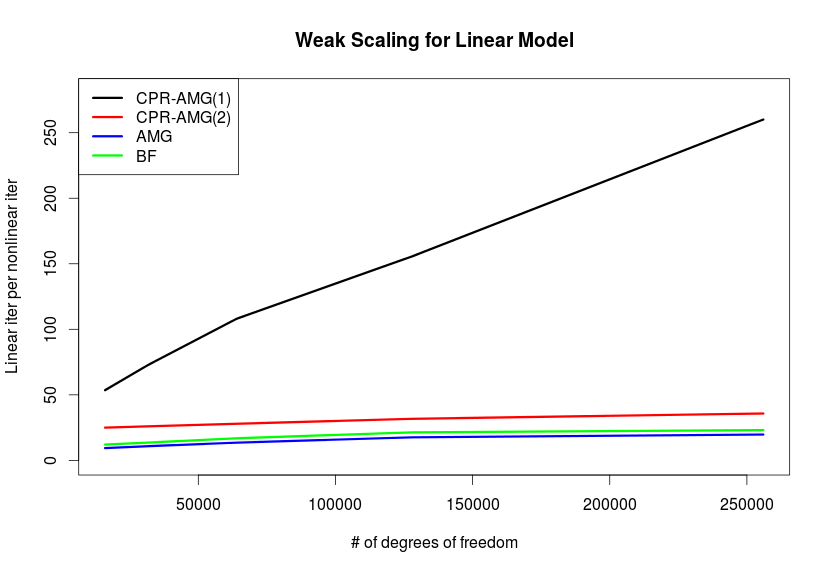
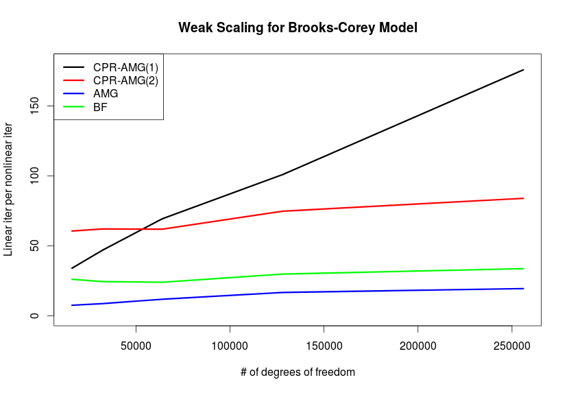
Figure 4: Weak scaling for different strategies.

The results shown in Figure 4. indicate that the performance of the block factorization, CPR-AMG(2), and AMG methods is independent of the mesh size. The number of linear iterations per Newton step does not grow as the mesh is refined which is optimal multigrid performance. The block factorization method’s performance is nearly identical to that of AMG for the linear model, and still quite close for the Brooks-Corey model, compared to CPR-AMG(2). CPR-AMG(1), however, does not scale as well as the other two methods. The linear iteration counts for CPR-AMG(1) grows linearly as the mesh is refined.

5 Conclusions

In this work, we have implemented a fully implicit parallel isothermal two-phase flow simulator along with four different preconditioning strategies to solve the linear systems resulting from linearization of the coupled equations, and we have tested the performance of these methods as preconditioners for GMRES. We have also developed a new block factorization preconditioner whose performance is robust and efficient across all benchmark problems studied. In contrast, although AMG preconditioning applied to the coupled systems is the most efficient choice in some cases (both two-dimensional and three-dimensional diffusion-dominated examples), it exhibits slow convergence and sometimes diverges for advection-dominated cases. The new block factorization preconditioner achieves consistently low iteration counts across all the tests and varying examples of capillary pressure, and it scales optimally with problem size. The combinative CPR-AMG(1), though robust across all the tests, is the least efficient method, with the exception of the near hyperbolic case where it is faster than CPR-AMG(2). The additive CPR-AMG(2) method performs well in most cases except the strongly advection-dominated case. It also scales optimally with problem size for both advection-dominated and diffusion-dominated case.

References

- [1] ASCEM. http://esd.lbl.gov/research/projects/ascem/thrusts/hpc/, 2009.
- [2] O. Axelsson. Iterative Solution Methods. Cambridge University Press, 1994.
- [3] K. Aziz and A. Settari. Petroleum Reservoir Simulation. Applied Science Publishers, 1979.
- [4] P. Bastian. Numerical computation of multiphase flow in porous media. Habilitationsschrift, 1999.
- [5] P. Bastian and R. Helmig. Efficient fully-coupled solution techniques for two-phase flow in porous media: Parallel multigrid solution and large scale computations. Advances in Water Resources, 23(3):199 – 216, 1999.
- [6] A. Behie and P.K.W. Vinsome. Block iterative methods for fully implicit reservoir simulation. Society of Petroleum Engineers Journal, 22(05):658–668, oct 1982.
- [7] R. Brooks and A. Corey. Hydraulic Properties of Porous Media. Hydrology Papers, Colorado State Univeristy, 1964.
- [8] M.A. Christie and M.J. Blunt. Tenth SPE comparative solution project: A comparison of upscaling techniques. In SPE Reservoir Simulation Symposium. Society of Petroleum Engineers (SPE), 2001.
- [9] A.J. Cleary, R.D. Falgout, V.E. Henson, and J.E. Jones. Coarse-grid selection for parallel algebraic multigrid. In Alfonso Ferreira, José Rolim, Horst Simon, and Shang-Hua Teng, editors, Solving Irregularly Structured Problems in Parallel, volume 1457 of Lecture Notes in Computer Science, pages 104–115. Springer Berlin Heidelberg, 1998.
- [10] T. Clees and L. Ganzer. An efficient algebraic multigrid solver strategy for adaptive implicit methods in oil-reservoir simulation. SPE Journal, 15(03):670–681, 2010.
- [11] E. Coon, J. D. Moulton, and S. Painter. Managing complexity in simulations of land surface and near-surface processes. Technical Report LA-UR 14-25386, Applied Mathematics and Plasma Physics Group, Los Alamos National Laboratory, 2014.
- [12] A. T. Corey. Mechanics of Immiscible Fluids in Porous Media. Water Resources Pubns, 1995.
- [13] C.N. Dawson, H. Klie, M.F. Wheeler, and C.S. Woodward. A parallel, implicit, cell-centered method for two-phase flow with a preconditioned Newton–Krylov solver. Computational Geosciences, 1(3-4):215–249, 1997.
- [14] R.D. Falgout, J.E. Jones, and U.M. Yang. The design and implementation of hypre, a library of parallel high performance preconditioners. In AreMagnus Bruaset and Aslak Tveito, editors, Numerical Solution of Partial Differential Equations on Parallel Computers, volume 51 of Lecture Notes in Computational Science and Engineering, pages 267–294. Springer Berlin Heidelberg, 2006.
- [15] R.D. Falgout and U.M. Yang. HYPRE: a library of high performance preconditioners. In Preconditioners,” Lecture Notes in Computer Science, pages 632–641, 2002.
- [16] V.E. Henson and U.M. Yang. BoomerAMG: a parallel algebraic multigrid solver and preconditioner. Applied Numerical Mathematics, 41:155–177, 2000.
- [17] H. Klie, M. Rame, and M.F. Wheeler. Two-stage preconditioners for inexact Newton methods in multiphase reservoir simulation. Technical report, Center for Research on Parallel Computation, Rice University, 1996.
- [18] S. Lacroix, Yu. Vassilevski, J. Wheeler, and M.F. Wheeler. Iterative solution methods for modeling multiphase flow in porous media fully implicitly. SIAM J. Sci. Comput., 25(3):905–926, jan 2003.
- [19] B. Lu. Iteratively Coupled Reservoir Simulation for Multiphase Flow in Porous Media. PhD thesis, Center for Subsurface Modeling, ICES, The University of Texas - Austin, 2008.
- [20] R. Masson, R. Scheichl, P. Quandalle, C. Guichard, R. Eymard, R. Herbin, and K. Brenner et al. CPR-AMG preconditioner for multiphase porous media flows: a few experiments. La page numérique du LATP - UMR 7353- Marseille, 2012.
- [21] D. Osei-Kuffuor, L. Wang, R. D. Falgout, and I. D. Mishev. An algebraic multigrid solver for fully-implicit solution methods in reservoir simulation. SIAM Geosciences, Society for Industrial and Applied Mathematics (SIAM), 2015.
- [22] S.V Patankar and D.B Spalding. A calculation procedure for heat, mass and momentum transfer in three-dimensional parabolic flows. International Journal of Heat and Mass Transfer, 15(10):1787 – 1806, 1972.
- [23] D.W. Peaceman. Fundamentals of Numerical Reservoir Simulation. Elsevier, Amsterdam, 1977.
- [24] PetroWiki. Relative permeability models. http://petrowiki.org/Relative_permeability_models.
- [25] J. W. Ruge and K. Stueben. 4. Algebraic Multigrid, chapter 4, pages 73–130. 1986.
- [26] T. F. Russell and M.F. Wheeler. Finite element and finite difference methods for continuous flows in porous media. In The Mathematics of Reservoir Simulation, chapter 2, pages 35–106. Society for Industrial and Applied Mathematics, 1983.
- [27] Y. Saad. Iterative Methods for Sparse Linear Systems. Society for Industrial and Applied Mathematics, second edition, 2003.
- [28] Y. Saad and M.H. Schultz. GMRES: A generalized minimal residual algorithm for solving nonsymmetric linear systems. SIAM J. Sci. Stat. Comput., 7(3):856–869, July 1986.
- [29] K. Stueben. A review of algebraic multigrid. Journal of Computational and Applied Mathematics, 128(1–2):281 – 309, 2001. Numerical Analysis 2000. Vol. VII: Partial Differential Equations.
- [30] K. Stueben, T. Clees, H. Klie, B. Lu, and M.F. Wheeler. Algebraic multigrid methods (AMG) for the efficient solution of fully implicit formulations in reservoir simulation. In SPE Reservoir Simulation Symposium. Society of Petroleum Engineers (SPE), 2007.
- [31] J.R. Wallis, R.P. Kendall, and L.E. Little. Constrained residual acceleration of conjugate residual methods. 1985.
- [32] J.W. Watts. A compositional formulation of the pressure and saturation equations. In SPE Reservoir Simulation Symposium. Society of Petroleum Engineers (SPE), SPE 12244, 1985.
- [33] Joshua A. White and Ronaldo I. Borja. Block-preconditioned Newton–Krylov solvers for fully coupled flow and geomechanics. Computational Geosciences, 15(4):647–659, 2011.
- [34] U.M. Yang. Parallel algebraic multigrid methods — high performance preconditioners. In Numerical Solution of Partial Differential Equations on Parallel Computers, volume 51 of Lecture Notes in Computational Science and Engineering, pages 209–236. Springer Berlin Heidelberg, 2006.