Overcoming strong metastabilities with the LLR method

Abstract:

In previous work, it has been shown that the recently proposed LLR method is very efficient at overcoming strong metastabilities that arise near first-order phase transition points. Here we present a systematic study of the performance of the algorithm near (pseudo-)critical points for $q$-state Potts models with $q$ as large as 20, in two and three dimensions. In particular, we shall focus our study on the ergodicity of the replica exchange step and the underlying physical mechanism. When compared with both analytical and numerical results present in the literature, our determinations of thermodynamic observables (including the order-disorder interface tension at criticality) show an impressive degree of relative accuracy (up to $2.5\times 10^{-6}$), which confirms the reliability and the efficiency of the proposed approach.

1 Introduction: the LLR algorithm and ergodicity through replica exchange

The LLR algorithm was originally introduced in [1] as an extension of the ideas behind the Wang-Landau sampling [2] allowing us to efficiently extract the density of states in systems with a continuous energy spectrum. Following further developments, this algorithm has shown a range of applicability that encompasses a rich variety of problems in lattice gauge theories and statistical mechanics, including exponentially growing tunneling times at first order phase transitions [3] and the sign problem [4].

The LLR algorithm determines numerically the density of states of a system using a non-Markovian sampling. A key aspect of the approach is the sequencing of the whole energy spectrum in intervals of amplitude $\delta$, assumed to be small enough for the logarithm of the density of states to be accurately approximated by its first order Taylor expansion. The latter is then determined with a recursive relation including steps of standard Monte Carlo sampling, with the constraint that the system never leaves the given energy interval. A review of the method, which we use in the formulation given in [3], has been provided at this conference [5]. Here we focus our attention on the energy restricted Monte Carlo. One of the potential problems with restricting the energy interval consists in a possible loss of ergodicity, which would invalidate the numerical results obtained with the algorithm. While one might assume that the restricted energy Monte Carlo explores all the configurations associated with the given energy range, that is not necessarily the case. In fact, there are scenarios in which the configuration space can become disconnected if one restricts the sampling in the energy (e.g. when the system has some non-trivial topological sectors).

Figure 1: The two sequences of overlapping intervals covering the whole energy range. The case of a coincidence of two energies $E_{i_{2n}}$ and $E_{i_{2n}-1}$ in an overlapping region is also sketched.

In order to overcome this problem, in [3] a replica exchange step has been proposed. The proposal consists in having a second sequence of energy intervals displaced from the original one by half an interval (Fig. 1). After a certain number of restricted Monte Carlo steps, when in two overlapping intervals (which we call $i_{2n-1}$ and $i_{2n}$) both configurations are in the overlapping region, one proposes a swap of configurations with a Metropolis probability

$$P_{\mathrm{swap}}=\mathrm{min}\left(1,e^{\left(a^{(m)}_{i_{2n}}-a^{(m)}_{i_{2n-1}}\right)\left(E_{i_{2n}}-E_{i_{2n-1}}\right)}\right)\ .$$ (1)

In this expression, $a^{(m)}_{i_{2n}}$ (respectively, $a^{(m)}_{i_{2n-1}}$) is the current iterative estimate of the first Taylor coefficient in the interval $i_{2n}$ ($i_{2n-1}$) and $E_{i_{2n}}$ ($E_{i_{2n-1}}$) the energy of the configuration in $i_{2n}$ ($i_{2n-1}$). Via subsequent swaps, the system can travel through the whole energy range, hence solving any potential ergodicity issue. A test that would enable us to verify whether this idea works in practice would be to establish that at convergence the system moves across intervals following a random walk, as it happens in the Wang-Landau algorithm.

In this work, we study numerically the replica exchange idea for the first time, using as a prototype the $q$-state Potts model (see [7] for a formulation of the LLR method for spin systems) in two and three dimensions and for $q$ as large as 20.

2 Application to the Potts model

Figure 2: The average energy per unit site as a function of $\beta$ for $D=2$, $L=64$ (left) and $D=3$, $L=16$ (right), at the shown $q$ values. The vertical lines indicate the position of $\beta_{c}$.

The Hamiltonian of the $q$-state Potts model in $D$ dimensions is given by

$$H=2\beta\sum_{\langle ij\rangle}\left(\frac{1}{q}-\delta_{\sigma_{i},\sigma_{j}}\right)\ ,$$ (2)

with the spin variables $\sigma_{i}$ taking the values $0,\dots,q-1$ and the sum ranging over all lattice links. The lattice is symmetric, with linear size $L$ and volume $V=L^{D}$.

For $D>1$, as a function of the coupling $\beta$, the system has a $\mathbb{Z}_{q}$-driven phase transition. In $D=2$ the $q$-state Potts model (which for $q=2$ is equivalent to the Ising model) has a first order phase transition for $q>4$, while in $D=3$ the transition is first order for $q>2$. In both cases, the strength of the transition grows significantly with $q$. In $D=2$ the $q=10$ case is generally taken as a benchmark of efficiency of algorithms [2], while the highest value of $q$ simulated we are aware of is $q=30$ [8]. For $D=3$ accurate Multicanonical Monte Carlo results have been presented in [9] up to $q=10$. Both known analytic results (for $D=2$) and precise numerical calculations already reported in the literature provide a solid reference base against which novel numerical approaches like ours can be assessed.

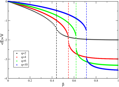
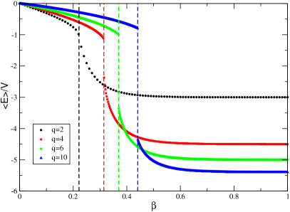
As a first check of our method, we verify that the energy as a function of $\beta$ has the expected behaviour, i.e. it goes to zero in the limit $\beta\to 0$ and to $4(1-q)/q$ in the limit $\beta\to\infty$, with clear indication of the phase transition arising at $\beta_{c}$. This is shown in Fig. 2, in which we plot the energy per unit site as a function of $\beta$ for $q=2,4,6,10$. In $D=2$ we have used square lattices of linear size $L=64$, while in $D=3$ we have simulated cubic lattices with $L=16$. The critical values of $\beta$ used for this test, also reported in the figure, are the exact infinite size values in two dimensions,

$$\beta_{c}=\frac{1}{2}\log\left(1+\sqrt{q}\right)\ ,$$ (3)

and the numerical extrapolations to $L=\infty$ reported in [9] for three dimensions. The figure supports the correctness of our simulation approach. In particular, the would-be infinite volume singularity at $\beta_{c}$ is well visible, with clear indication of a jump in the thermodynamic limit at the largest values of $q$.

Figure 3: Left: A Monte Carlo history of the action $A=\sum_{\langle ij\rangle}\delta_{\sigma_{i},\sigma_{j}}$ of the system evolved from a configuration in the displayed central energy interval with the replica exchange step enabled. The dark and light blue bands visualise the energy intervals. Right: Quadratic fit of the diffusion length as a function of the Monte Carlo time.

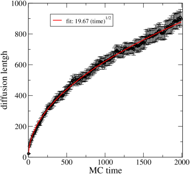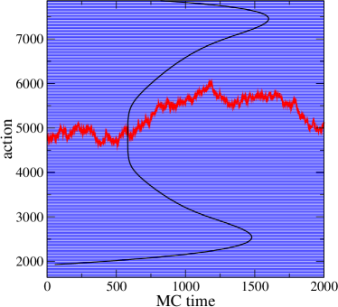
Next, we analyse more directly the dynamics provided by the replica exchange. As a first investigation, we follow the history of a configuration originally having energy in an interval that is in between the two peak values at criticality. In this region of energies, an interface separating the two phases (the ordered and the disordered phase) develops near the critical temperature. This study is performed for $q=20$ and $D=2$. As the replica exchange step is turned on, the system is found to be travelling in energy space in a fashion that is clearly reminiscent of a random walk (Fig. 3). We then fit the diffusion mean length $E_{d}=\langle(E-E_{0})^{2}\rangle^{1/2}$ using the random walk law

$$E_{d}=C_{d}t_{MC}^{1/2}\ ,$$ (4)

where $t_{MC}$ is the Monte Carlo time and $C_{d}$ the diffusion coefficient. In this particular case, we find $C_{d}\simeq 19.67$. The quality of the fit is displayed in Fig. 3, right. $C_{d}$ seems to be independent of the starting energy: for an energy that corresponds to an equilibrium value in the ordered phase we find $C_{d}\simeq 18.73$, while for an energy corresponding to an equilibrium value in the disordered phase we find $C_{d}\simeq 19.80$. This suggests that our algorithm produces a random walk over all energies, hence avoiding any trapping that can result from the original LLR prescription.

Figure 4: Left: The logarithm of the probability distribution of the energy per unit site as a function of the latter quantity at $\beta_{c}^{P}(L)$. Right: Infinite volume extrapolation of $\beta_{c}^{P}(V^{-1})\equiv\beta_{c}^{P}(L=V^{1/2})$.

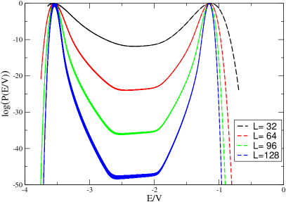
We then move to a quantitative analysis of the phase transition. Also for this study, we consider the Potts model with $q=20$. Due to the severe metastabilities in the critical region, this investigation is expected to provide a compelling test of the efficiency of the algorithm at first order phase transition points. We start our numerical study from the identification of the critical value of the coupling $\beta_{c}$. At finite size, various definitions of $\beta_{c}(L)$ are possible, which do not necessarily identify the same value at fixed $L$, but all converge to a unique $\beta_{c}$ when $L\to\infty$. Here, we choose to identify $\beta_{c}(L)$ with $\beta_{c}^{P}(L)$, the value of $\beta$ at which the probability distribution of the energy per unit site $P(E/V)$ has two peaks of equal height. A plot in logarithmic scale of $P(E/V)$ is reported in Fig. 4 (left). We note the presence of a flat valley between the two maxima, whose depth increases as $L$ is increased. The latter is the feature that ultimately leads to the failure of local update algorithms at first order phase transitions, since in order to travel through the valley one would need a simulation time that grows exponentially with $L^{D-1}$. The visual indication from the plot is that our algorithm does allow us to sample efficiently the metastable vacua and the mixed phase configurations that characterise the valley.

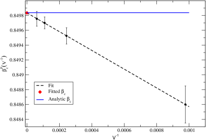
In order to have a more stringent quantitative test, we extract the critical values $\beta_{c}(L)$ using a bootstrap analysis on 20 different simulations. The latter have been performed feeding independent Markov chains to the LLR algorithm.

The system having a first order phase transition, finite size scaling predicts that

$$\beta_{c}^{P}(L)=\beta_{c}+\frac{A}{L^{D}}\ ,$$ (5)

with $A$ a constant. Our determinations of $\beta_{c}(L)$ are displayed in the right pane of Fig. 4 together with the expected linear dependency in $V^{-1}=L^{-D}$. Beside an obvious overestimate of the errors (whose understanding is a work in progress), the excellent quality of the fit is evident. The extracted numerical value is $\beta_{c}^{fit}=0.8498350(21)$, which is perfectly compatible with the $q=20$ value coming from the exact expression, Eq. (3 ). More in details,

$$\frac{\beta_{c}^{fit}-\beta_{c}^{exact}}{\beta_{c}^{exact}}=1.7(2.5)\times 10^{-6}\ ,$$ (6)

i.e. the compatibility is verified up to a statistical error that is 2.5 parts per million. Not only does this analysis demonstrate the efficiency of the algorithm, but it also shows the high level of accuracy that it allows us to obtain.

Figure 5: The finite-$L$ interface tension $\sigma_{od}(L)$ as a function of the size for $q=20$ and $D=2$. The infinite $L$ extrapolation is also provided.

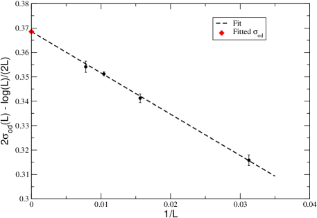
The tension of the interface between ordered and disordered phase is an observable that plays an important role at first order phase transitions (see e.g. [10]). This quantity can be extracted from the relative height between the two equal peaks and the minimum in the flat region between them at $\beta_{c}^{P}(L)$. In particular, if we define the interface tension $\sigma_{od}$ from

$$2\sigma_{od}(L)=-\frac{1}{L}\log P_{min,valley}\ ,$$ (7)

where the peak probability has been normalised to one, the latter can be extrapolated to infinite $L$ using the ansatz

$$2\sigma_{od}(L)-\frac{\log L}{2L}=2\sigma_{od}+\frac{c_{\sigma}}{L}\ ,$$ (8)

where $\frac{\log L}{2L}$ is an entropic term due to the fact that the system is translationally invariant along the direction of the interface. Our data are displayed in Fig. 5, where we show also the best fit according to (8). For the infinite volume value, we obtain $2\sigma_{od}=0.36853(88)$. This can be compared to the strong coupling analytic result of Borgs and Janke [11], which, for $q=20$, gives $2\sigma_{od}=0.3709881649\dots$. The relative discrepancy of the two results is of the order of $7\times 10^{-3}$. While there is no reason to expect perfect agreement, since the analytic result is not exact (although is known to provide a very good approximation to the exact value) and the numerical result is still preliminary, it is reassuring for our purposes that the numbers are close at the sub-percent level. Further analysis will be performed to check the robustness of our determination.

3 Conclusions

In this contribution, we have shown that the LLR method provides an efficient numerical tool for investigating strong metastabilities at first order phase transitions even in the case of the Potts model, for which the energy spectrum is discrete. In particular, the replica exchange method plays a crucial role in extending the random walk from the single interval in which the simulation is requested to be restricted by the LLR original prescription to the whole energy range. The provided verification of the random walk dynamic of the Monte Carlo time series supports the conjecture that the algorithm scales as $V^{2}$ also in the case of a first order phase transition. This has to be contrasted with Markov Chain Monte Carlo methods, for which the scaling is known to be exponential in $L^{d-1}$. It is worth remarking that the results presented here have been obtained with modest computational times (three weeks of runs on around 200 cores of state of the art processors). We regard this study as preliminary. A detailed study of some aspects only hinted in this work (among which is the scaling of the algorithm with the system size) is the focus of our current investigation and will be reported elsewhere.