Wall-Bounded Multiphase Flows of $N$ Immiscible Incompressible Fluids: Consistency and Contact-Angle Boundary Condition

Abstract

We present an effective method for simulating wall-bounded multiphase flows consisting of $N$ ($N\geqslant 2$) immiscible incompressible fluids with different densities, viscosities and pairwise surface tensions. The N-phase physical formulation is based on a modified thermodynamically consistent phase field model that is more general than in a previous work, and it is developed by considering the reduction consistency if some of the fluid components were absent from the system. We propose an N-phase contact-angle boundary condition that is reduction consistent between $N$ phases and $M$ phases ($2\leqslant M\leqslant N-1$). We also present a numerical algorithm for solving the N-phase governing equations together with the contact-angle boundary conditions developed herein. Extensive numerical experiments are presented for several flow problems involving multiple fluid components and solid-wall boundaries to investigate the wettability effects with multiple types of contact angles. In particular, we compare simulation results with the de Gennes theory for the contact-angle effects on the liquid drop spreading on wall surfaces, and demonstrate that our method produces physically accurate results.

Keywords: Contact angles; N-phase contact angles; reduction consistency; pairwise surface tensions; phase field; multiphase flow;

1 Introduction

In the present work we focus on the motion of a mixture of $N$ ($N\geqslant 2$) immiscible incompressible fluids with different physical properties (such as densities, dynamic viscosities, and pair-wise surface tensions) within a domain bounded by solid walls. Moving contact lines form on the solid wall where fluid interfaces intersect the wall surface, and the wall wettability, characterized by the contact angles, can significantly influence the dynamics and the equilibrium state of the system. Following the notation of our previous works Dong2014 ; Dong2015 , we refer to such problems as N-phase flows, where N refers to the number of different fluid components in the system. Due to the multitude of different types of fluid interfaces in the system, wall-bounded N-phase flows can potentially accommodate a large number of different types of contact lines and different contact angles on the wall. Potential applications of wall-bounded multiphase flows are enormous, in e.g. materials processing, microfluidic devices, and functional surfaces.

We primarily consider N-phase systems involving three or more fluid components (i.e. $N\geqslant 3$) in the current work, and our approach falls into the phase field (or diffuse interface) framework. Our attention below and in subsequent sections of this paper will therefore be confined to this approach. For two-phase flows one can refer to e.g. AndersonMW1998 ; SethianS2003 ; Tryggvasonetal2001 ; ScardovelliZ1999 for a review of this and related approaches. The developments for three or more fluid phases have been contributed by a number of researchers; see e.g. KimL2005 ; BoyerL2006 ; Kim2009 ; BoyerLMPQ2010 ; BoyerM2011 ; Kim2012 ; HeidaMR2012 ; ZhangW2016 . Among these, two phase field models are developed in KimL2005 ; HeidaMR2012 based on the mass-averaged velocity, which is not divergence free. The constitutive relations therein are formulated based on thermodynamic considerations such as the maximization of entropy production. The study of a three-phase model in BoyerL2006 signifies the importance in the choice of the free energy form. More interestingly, the authors thereof have proposed several natural reduction consistency conditions that three-phase models should satisfy.

More recently, we have proposed in Dong2014 a general phase field model for formulating the motion of an isothermal mixture of $N$ ($N\geqslant 2$) immiscible incompressible fluids (see also Section 1.1 below). The model is derived by considering the mass conservations of the N individual fluid components, the momentum conservation, the second law of thermodynamics, and the Galilean invariance principle. Our model is based on a volume-averaged mixture velocity, which can be rigorously shown to be divergence free Dong2014 . Therefore, it is fundamentally different from those of KimL2005 ; HeidaMR2012 . This N-phase model involves a free energy density function and ($N-1$) independent order parameters (or interchangeably phase field variables). It is a general model in the sense that the free energy density function and the set of ($N-1$) independent order parameters remain to be specified. Once the form of the free energy density function and a set of order parameters are specified, the model will give rise to a specific physical formulation for the N-phase system. In Dong2014 ; Dong2015 , by employing a specific form for the free energy density function and choosing a set of order parameters, we have derived from the general model specific physical formulations for incompressible N-phase flows. We have further devised associated numerical algorithms for their simulations.

In an interesting work BoyerM2014 Boyer and collaborator have recently generalized the reduction consistency conditions of BoyerL2006 from three phases to more general N phases, and provided an in-depth discussion of the effects of these conditions on the modeling of N-phase systems, in particular, on the choice of N-phase free energy density function. More specifically, they have looked into the following three consistency properties:

1. The N-phase free energy density function should coincide with the two-phase free energy density function if $N=2$;

2. If only a set of $M$ ($2\leqslant M\leqslant N-1$) fluids are present in the system, then the N-phase free energy density function should reduce to the corresponding $M$-phase free energy density function;

3. If $K$ ($1\leqslant K\leqslant N-2$) fluid phases are absent from the initial data, then they should remain absent in the N-phase solution over time.

These consistency conditions, and in particular property ($\mathscr{C}$3), stringently restrict the form of the free energy density function, and especially the potential free energy form (i.e. “multiwell” potential). It is shown in BoyerM2014 that, given an arbitrary set of pair-wise surface tension values, it is extremely challenging to construct an N-phase potential free energy that fully satisfies ($\mathscr{C}$3) with arbitrary $1\leqslant K\leqslant N-2$. The existence of such an N-phase potential energy for a general set of pair-wise surface tensions is still an open problem. Several possible potential energy forms with interesting properties, as well as other related function forms are explored in BoyerM2014 .

Inspired by the consistency conditions of BoyerM2014 , we have looked into the N-phase free energy density function employed in our previous works Dong2014 ; Dong2015 and the resultant N-phase physical formulations. The specific form of the N-phase potential free energy function employed therein satisfies the consistency properties ($\mathscr{C}$1) and ($\mathscr{C}$2). However, when combined with the N-phase governing equations, it appears to fall short with respect to ($\mathscr{C}$3). This inadequacy motivates the work in the current paper.

In this paper, we present developments in the following aspects:

• We specify, when developing the N-phase model, a different constitutive relation than that of Dong2014 to ensure the second law of thermodynamics. This leads to a modified phase field model that is more general than that of Dong2014 .

• We combine the modified N-phase model and the consistency considerations as discussed in BoyerM2014 to develop specific N-phase physical formulations to improve the reduction consistency.

• We propose an N-phase contact angle boundary condition that is reduction consistent between $N$ phases and $M$ phases ($2\leqslant M\leqslant N-1$).

• We develop a numerical algorithm for solving the N-phase governing equations together with the N-phase contact-angle boundary condition developed herein.

More specifically, besides the afore-mentioned consistency properties ($\mathscr{C}$1), ($\mathscr{C}$2) and ($\mathscr{C}$3), we also consider two additional consistency conditions in the current work:

1. If only a set of $M$ ($2\leqslant M\leqslant N-1$) fluids are present in the system, then the $N$-phase governing equations should reduce to those for the corresponding $M$-phase system.

2. If only a set of $M$ ($2\leqslant M\leqslant N-1$) fluids are present in the system, then the boundary conditions for the N-phase system should reduce to those for the corresponding $M$-phase system.

Note that the above condition ($\mathscr{C}$4) imposes a stronger consistency requirement on the N-phase formulation than ($\mathscr{C}$3) in two aspects: (i) The condition ($\mathscr{C}$4) includes consistency requirements on the momentum equations, in addition to the phase field equations. (ii) The condition ($\mathscr{C}$4) requires not only that the fluid phases initially absent should remain absent over time, but also that the governing equations for the fluid phases that are present in the system should reduce to the corresponding ones for the smaller system excluding the fluid phases that are absent. One should also note that, in order to satisfy the consistency properties ($\mathscr{C}$2)–($\mathscr{C}$5) between the N-phase system and an $M$-phase system ($2\leqslant M\leqslant N-1$), it suffices to consider only the reduction from the N-phase system to the ($N-1$)-phase system, that is, if any one fluid phase is absent from the N-phase system.

Employing the N-phase formulation resulting from the above discussions, we look into the N-phase contact angle boundary conditions on solid-wall boundaries. In principle, the interface formed between any pair of these $N$ fluids can intersect the wall and form a contact angle thereupon. So potentially $\frac{1}{2}N(N-1)$ different contact angles can exist on the wall in the N-phase system. However, among them only ($N-1$) contact angles are independent due to the Young’s relations Blunt2001 . Once the ($N-1$) independent contact angles are provided, all the other contact angles at the wall can be determined based on the Young’s equations. As mentioned earlier, ($N-1$) independent phase field variables are involved in our N-phase model, which is consistent with the existence of ($N-1$) independent contact angles in the N-phase system. We develop a reduction consistent contact-angle boundary condition by imposing the requirement that the boundary condition should satisfy the consistency property ($\mathscr{C}$5). In the current paper our attention will be restricted to equilibrium (or static) contact angles only. We note that it is not difficult to extend these conditions to account for the dynamic effect, by for example incorporating appropriate inertial terms. Contact angles in flows with two or three fluid phases are considered in a number of previous studies; see e.g. Jacqmin2000 ; YueZF2010 ; YueF2011 ; CarlsonDA2011 ; Dong2012 ; ShiW2014 ; ZhangW2016 .

The novelties of this paper lie in three aspects: (i) the modified (more general) phase field model presented herein; (ii) the N-phase physical formulation resulting from the modified phase field model and the consistency considerations; (iii) the reduction consistent N-phase contact-angle boundary conditions. While the numerical algorithm for the phase field equations presented herein can also be considered new, the strategies for dealing with the several numerical issues therein are straightforward adaptations from those developed in DongS2012 ; Dong2014 .

The rest of this paper is structured as follows. In the rest of this section we summarize the key points of the phase field model developed in Dong2014 . Then in Section 2 we present a modified phase field model, and develop an N-phase physical formulation by considering the consistency conditions ($\mathscr{C}$1)–($\mathscr{C}$5). We present in Section 3 a consistent N-phase contact-angle boundary condition, and in Section 4 a numerical algorithm for solving the N-phase governing equations together with the contact-angle boundary condition. After that we demonstrate the performance of the method developed herein using several flow problems involving multiple fluid components and solid walls in Section 5. In particular we compare simulations with the de Gennes theory deGennesBQ2003 to show the accuracy of the simulation results. We also look into the effects of the various contact angles on the equilibrium configuration and the dynamics of the system when multiple fluid components are involved. Section 6 concludes the discussions with a summary of the key points. In the appendices we provide proofs to several theorems from the main body of the text, and also provide a summary of the numerical algorithm for solving the momentum equations.

1.1 A Phase Field Model for N-Fluid Mixture

In Dong2014 we have derived a general phase field model for the isothermal system consisting of $N$ ($N\geqslant 2$) immiscible incompressible fluids based on thermodynamic principles, namely, the conservations of mass and momentum, the Galilean invariance principle, and the second law of thermodynamics; see the Appendix of Dong2014 for the detailed derivation of this model. We summarize below several key points in the development of this model, which are crucial to subsequent developments in the current paper.

Consider the mixture of $N$ ($N\geqslant 2$) immiscible incompressible fluids contained in some flow domain $\Omega$ (domain boundary denoted by $\partial\Omega$). Let $\tilde{\rho}_{i}$ and $\tilde{\mu}_{i}$ ($1\leqslant i\leqslant N$) denote the constant densities and constant dynamic viscosities of these $N$ pure fluids (before mixing). Define auxiliary parameters

$$\tilde{\gamma}_{i}=\frac{1}{\tilde{\rho}_{i}},\ 1\leqslant i\leqslant N;\quad\Gamma=\sum_{i=1}^{N}\tilde{\gamma}_{i};\quad\Gamma_{\mu}=\sum_{i=1}^{N}\frac{\tilde{\mu}_{i}}{\tilde{\rho}_{i}}.$$ (1)

Let $\phi_{i}$ ($1\leqslant i\leqslant N-1$) denote the ($N-1$) independent order parameters, or interchangeably the phase field variables, that characterize the system, and $\vec{\phi}=(\phi_{1},\dots,\phi_{N-1})$. Let $\rho_{i}(\vec{\phi})$ and $c_{i}(\vec{\phi})$ ($1\leqslant i\leqslant N$) denote the density and volume fraction of fluid $i$ within the mixture, and let $\rho(\vec{\phi})$ denote the density of the N-phase mixture. Then we have the relations Dong2014

$$c_{i}=\frac{\rho_{i}}{\tilde{\rho}_{i}},\ 1\leqslant i\leqslant N;\quad\sum_{i=1}^{N}c_{i}=1;\quad\rho=\sum_{i=1}^{N}\rho_{i}.$$ (2)

The mass balance of the $N$ individual fluid phases is described by the $(N-1)$ independent mass balance equations Dong2014

$$\frac{\partial}{\partial t}\left(\rho_{i}-\rho_{N}\right)+\mathbf{u}\cdot\nabla\left(\rho_{i}-\rho_{N}\right)=-\nabla\cdot\mathbf{J}_{ai},\quad 1\leqslant i\leqslant N-1,$$ (3)

where $\rho_{i}$ ($1\leqslant i\leqslant N$) is the density of fluid $i$ within the mixture, and $\mathbf{u}$ is the volume averaged mixture velocity and can be rigorously shown to be divergence free Dong2014

$$\nabla\cdot\mathbf{u}=0.$$ (4)

$\mathbf{J}_{ai}$ ($1\leqslant i\leqslant N-1$) are ($N-1$) diffusive fluxes whose forms are to be determined based on the second law of thermodynamics.

The momentum balance of the system is described by Dong2014

$$\rho\left(\frac{\partial\mathbf{u}}{\partial t}+\mathbf{u}\cdot\nabla\mathbf{u}\right)+\tilde{\mathbf{J}}\cdot\nabla\mathbf{u}=-\nabla p+\nabla\cdot\mathbf{S},$$ (5)

where $p$ is the pressure, and $\mathbf{S}$ is a stress tensor whose form is to be determined based on the second law of thermodynamics. The density of fluid $i$ within the mixture $\rho_{i}$, the volume fraction $c_{i}$, and the mixture density $\rho$, are given by

$$\left\{\begin{split}&\rho_{i}(\vec{\phi})=\frac{1}{\Gamma}+\sum_{j=1}^{N-1}\left(\delta_{ij}-\frac{\tilde{\gamma}_{j}}{\Gamma}\right)\varphi_{j}(\vec{\phi}),\quad 1\leqslant i\leqslant N,\\ &c_{i}(\vec{\phi})=\tilde{\gamma}_{i}\rho_{i}(\vec{\phi})=\frac{\tilde{\gamma}_{i}}{\Gamma}+\sum_{j=1}^{N-1}\left(\tilde{\gamma}_{i}\delta_{ij}-\frac{\tilde{\gamma}_{i}\tilde{\gamma}_{j}}{\Gamma}\right)\varphi_{j}(\vec{\phi}),\quad 1\leqslant i\leqslant N,\\ &\rho(\vec{\phi})=\sum_{i=1}^{N}\rho_{i}=\frac{N}{\Gamma}+\sum_{i=1}^{N-1}\left(1-\frac{N}{\Gamma}\tilde{\gamma}_{i}\right)\varphi_{i}(\vec{\phi}),\end{split}\right.$$ (6)

where $\delta_{ij}$ is the Kronecker delta, and

$$\varphi_{i}(\vec{\phi})\equiv\rho_{i}-\rho_{N},\quad 1\leqslant i\leqslant N-1.$$ (7)

The flux $\tilde{\mathbf{J}}$ is given by

$$\tilde{\mathbf{J}}=\sum_{i=1}^{N-1}\left(1-\frac{N}{\Gamma}\tilde{\gamma}_{i}\right)\mathbf{J}_{ai}.$$ (8)

We introduce a free energy density function $W(\vec{\phi},\nabla\vec{\phi})$ in the spirit of the phase field approach to account for the interfacial energy for the diffuse interfaces. The appropriate forms for $\mathbf{J}_{ai}$ in (3) and $\mathbf{S}$ in (5) are determined by invoking the second law of thermodynamics, which for isothermal systems requires that the following inequality should hold,

$$\frac{d}{dt}\int_{\Omega(t)}e(\mathbf{u},\vec{\phi},\nabla\vec{\phi})\leqslant P_{c}$$ (9)

where $\Omega(t)$ is an arbitrary volume that is transported with the mixture velocity $\mathbf{u}$, the total energy density function $e(\mathbf{u},\vec{\phi},\nabla\vec{\phi})$ is given by $e(\mathbf{u},\vec{\phi},\nabla\vec{\phi})=\frac{1}{2}\rho(\vec{\phi})|\mathbf{u}|^{2}+W(\vec{\phi},\nabla\vec{\phi}),$ and $P_{c}$ is the conventional power expended on $\Omega(t)$. This inequality is eventually reduced to (see Dong2014 for details)

$$-\left(\mathbf{S}+\sum_{i=1}^{N-1}\nabla\phi_{i}\otimes\frac{\partial W}{\partial\nabla\phi_{i}}\right):\frac{1}{2}\mathbf{D}(\mathbf{u})+\sum_{i=1}^{N-1}\nabla\mathcal{C}_{i}\cdot\mathbf{J}_{ai}\leqslant 0$$ (10)

where $\mathbf{D}(\mathbf{u})=\nabla\mathbf{u}+\nabla\mathbf{u}^{T}$, and $\mathcal{C}_{i}$ ($1\leqslant i\leqslant N-1$) are ($N-1$) effective chemical potentials given by the linear system

$$\sum_{j=1}^{N-1}\frac{\partial\varphi_{j}}{\partial\phi_{i}}\mathcal{C}_{j}=\frac{\partial W}{\partial\phi_{i}}-\nabla\cdot\frac{\partial W}{\partial(\nabla\phi_{i})}.\quad 1\leqslant i\leqslant N-1.$$ (11)

In Dong2014 the following constitutive relations are chosen to ensure the inequality (10)

$$\mathbf{J}_{ai}=-\tilde{m}_{i}(\vec{\phi})\nabla\mathcal{C}_{i},\quad 1\leqslant i\leqslant N-1$$ (12a)

$$\mathbf{S}+\sum_{i=1}^{N-1}\nabla\phi_{i}\otimes\frac{\partial W}{\partial\nabla\phi_{i}}=\mu(\vec{\phi})\mathbf{D}(\mathbf{u}),$$ (12b)

where $\tilde{m}_{i}(\vec{\phi})\geqslant 0$ and $\mu(\vec{\phi})\geqslant 0$ are non-negative quantities playing the roles of mobility and viscosity, respectively. With these constitutive relations, the momentum equation (5) and the mass balance equations (3) are transformed into

$$\rho\left(\frac{\partial\mathbf{u}}{\partial t}+\mathbf{u}\cdot\nabla\mathbf{u}\right)+\tilde{\mathbf{J}}\cdot\nabla\mathbf{u}=-\nabla p+\nabla\cdot\left[\mu(\vec{\phi})\mathbf{D}(\mathbf{u})\right]-\sum_{i=1}^{N-1}\nabla\cdot\left(\nabla\phi_{i}\otimes\frac{\partial W}{\partial\nabla\phi_{i}}\right),$$ (13)

$$\sum_{j=1}^{N-1}\frac{\partial\varphi_{i}}{\partial\phi_{j}}\left(\frac{\partial\phi_{j}}{\partial t}+\mathbf{u}\cdot\nabla\phi_{j}\right)=\nabla\cdot\left[\tilde{m}_{i}(\vec{\phi})\nabla\mathcal{C}_{i}\right],\qquad 1\leqslant i\leqslant N-1.$$ (14)

The general phase field model of Dong2014 for the N-phase system consists of equations (13), (4) and (14), in which $\mathcal{C}_{i}$ ($1\leqslant i\leqslant N-1$) are given by the linear system (11). The order parameters $\vec{\phi}$ are defined through equation (7) (see Dong2015 for a family of order parameters), and the form of the free energy density function $W(\vec{\phi},\nabla\vec{\phi})$ is yet to be specified. Once the functions $\varphi_{i}(\vec{\phi})$ ($1\leqslant i\leqslant N-1$) and the free energy density function $W(\vec{\phi},\nabla\vec{\phi})$ are specified, essentially all the other quantities in the model can be computed.

2 Modified N-Phase Model and Physical Formulation

2.1 A Modified General Phase Field Model for N-phase Mixture

The point of departure of the current work is in the choice of the constitutive relation (12a) for the fluxes $\mathbf{J}_{ai}$ involved in the mass balance equations. In the present paper we consider a modified constitutive relation,

$$\mathbf{J}_{ai}=-\sum_{j=1}^{N-1}\tilde{m}_{ij}(\vec{\phi})\nabla\mathcal{C}_{j},\quad 1\leqslant i\leqslant N-1,$$ (15)

where $\tilde{m}_{ij}(\vec{\phi})$ ($1\leqslant i,j\leqslant N-1$) are coefficients. We require that the matrix formed by these coefficients

$$\tilde{\mathbf{m}}=\begin{bmatrix}\tilde{m}_{ij}\end{bmatrix}_{(N-1)\times(N-1)}$$ (16)

be symmetric positive definite (SPD) to ensure the non-positivity of the second term on the left hand side of the inequality (10). Note that this constitutive relation is more general than (12a). By requiring that $\tilde{\mathbf{m}}$ be a diagonal matrix, one can reduce (15) to (12a). With the constitutive relation (15) the mass balance equations (3) are transformed into

$$\sum_{j=1}^{N-1}\frac{\partial\varphi_{i}}{\partial\phi_{j}}\left(\frac{\partial\phi_{j}}{\partial t}+\mathbf{u}\cdot\nabla\phi_{j}\right)=\sum_{j=1}^{N-1}\nabla\cdot\left[\tilde{m}_{ij}(\vec{\phi})\nabla\mathcal{C}_{j}\right],\qquad 1\leqslant i\leqslant N-1.$$ (17)

The equations (13), (4), and (17) constitute a modified phase field model for the N-phase system that is more general than the one from Dong2014 . This model similarly satisfies the thermodynamic principles: the conservations of mass and momentum, the second law of thermodynamics, and Galilean invariance. This new N-phase model is the basis for the developments in the current work.

In this new model, $\tilde{\mathbf{J}}$ in the momentum equation (13) is given by

$$\tilde{\mathbf{J}}=\sum_{i=1}^{N-1}\left(1-\frac{N}{\Gamma}\tilde{\gamma}_{i}\right)\mathbf{J}_{ai}=-\sum_{i,j=1}^{N-1}\left(1-\frac{N}{\Gamma}\tilde{\gamma}_{i}\right)\tilde{m}_{ij}\nabla\mathcal{C}_{j}.$$ (18)

Once the functions $W(\vec{\phi},\nabla\vec{\phi})$ and $\varphi_{i}(\vec{\phi})$ ($1\leqslant i\leqslant N-1$) are known, the chemical potentials $\mathcal{C}_{i}$ ($1\leqslant i\leqslant N-1$) are computed from the linear system (11), and the densities $\rho_{i}(\vec{\phi})$ ($1\leqslant i\leqslant N$), volume fractions $c_{i}(\vec{\phi})$, and $\rho(\vec{\phi})$ are computed based on (6). We assume that the mixture dynamic viscosity $\mu(\vec{\phi})$ is given by an analogous expression to that for the mixture density $\rho(\vec{\phi})$ as follows,

$$\mu(\vec{\phi})=\sum_{i=1}^{N}\tilde{\mu}_{i}c_{i}(\vec{\phi})=\frac{\Gamma_{\mu}}{\Gamma}+\sum_{i=1}^{N-1}\left(\tilde{\mu}_{i}-\frac{\Gamma_{\mu}}{\Gamma}\right)\tilde{\gamma}_{i}\varphi_{i}(\vec{\phi}).$$ (19)

The density $\rho(\vec{\phi})$ given by (6) and the flux $\tilde{\mathbf{J}}$ given by (18) satisfy the relation

$$\frac{\partial\rho}{\partial t}+\mathbf{u}\cdot\nabla\rho=-\nabla\cdot\tilde{\mathbf{J}}$$ (20)

thanks to equation (17). By using this relation and assuming that all flux terms vanish on the domain boundary, it can be shown that the model consisting of equations (13), (4) and (17) admits the following energy law

$$\frac{\partial}{\partial t}\int_{\Omega}\left[\frac{1}{2}\rho|\mathbf{u}|^{2}+W(\vec{\phi},\nabla\vec{\phi})\right]=-\int_{\Omega}\frac{\mu}{2}\|\mathbf{D}(\mathbf{u})\|^{2}-\int_{\Omega}\sum_{i,j=1}^{N-1}\tilde{m}_{ij}\nabla\mathcal{C}_{i}\cdot\nabla\mathcal{C}_{j}$$ (21)

where $\Omega$ denotes the flow domain and $\partial\Omega$ denotes its boundary.

The above N-phase model is a general phase field model. To arrive at a specific physical formulation suitable for numerical simulations, the model further requires

• the specification of a set of order parameters $\phi_{i}$ ($1\leqslant i\leqslant N-1$) through equation (7);

• the specification of the form of the free energy density function $W(\vec{\phi},\nabla\vec{\phi})$;

• the determination of the coefficients $\tilde{m}_{ij}$.

The order parameters for the N-phase system have been discussed extensively in Dong2015 , and a family of order parameters has been introduced therein. This family allows the use of many commonly-used physical variables (e.g. volume fractions, volume fractions differences, densities, density differences) to formulate the system. In the present paper we will employ the family of order parameters introduced in Dong2015 to the formulate the N-phase system. More specifically, we define the order parameters $\phi_{i}$ ($1\leqslant i\leqslant N-1$) according to Dong2015

$$\varphi_{i}\equiv\rho_{i}-\rho_{N}=\sum_{j=1}^{N}a_{ij}\phi_{j}+b_{i},\quad 1\leqslant i\leqslant N-1,$$ (22)

where $a_{ij}$ and $b_{i}$ ($1\leqslant i,j\leqslant N-1$) are prescribed constants such that the matrix

$$\mathbf{A}_{1}=\begin{bmatrix}a_{ij}\end{bmatrix}_{(N-1)\times(N-1)}$$ (23)

must be non-singular. By prescribing a set of $a_{ij}$ and $b_{i}$, one will define a specific set of order parameters $\phi_{i}$ ($1\leqslant N-1$). The coefficients $a_{ij}$ and $b_{i}$ for several most commonly-used formulations have been provided in Dong2015 , which correspond to employing several commonly-encountered physical variables as the order parameters $\phi_{i}$, In the following, the development of the physical formulation will be presented in terms of a general set of order parameters $\phi_{i}$ defined by (22). However, in the numerical simulations of this paper, we will use a specific formulation, which corresponds to using the volume fractions $c_{i}$ ($1\leqslant i\leqslant N-1$) as the order parameters, i.e.

$$\phi_{i}=c_{i},\quad\phi_{i}\in[0,1],\quad 1\leqslant i\leqslant N-1.$$ (24)

The coefficients $a_{ij}$ and $b_{i}$ for this formulation are given by (see Dong2015 )

$$a_{ij}=\tilde{\rho}_{i}\delta_{ij}+\tilde{\rho}_{N},\quad b_{i}=-\tilde{\rho}_{N},\quad 1\leqslant i,j\leqslant N-1,$$ (25)

where $\delta_{ij}$ is the Kronecker delta.

The specification of the free energy density function $W(\vec{\phi},\nabla\vec{\phi})$ and the determination of the coefficients $\tilde{m}_{ij}$ call for considerations of the consistency conditions ($\mathscr{C}$1)–($\mathscr{C}$4). We focus on $W(\vec{\phi},\nabla\vec{\phi})$ and $\tilde{m}_{ij}$ in the subsequent sections.

2.2 N-Phase Free Energy Density Function

To determine an appropriate form for the free energy density function $W(\vec{\phi},\nabla\vec{\phi})$ and the coefficients $\tilde{m}_{ij}$, we consider the set of consistency conditions ($\mathscr{C}$1)–($\mathscr{C}$4) and insist that the N-phase formulation should honor these conditions. In Dong2014 ; Dong2015 we have considered the consistency of the free energy density function between N-phase and two-phase systems, and derived an explicit form for the mixing energy density coefficients involved in the free energy density function therein. The consistency conditions considered in Dong2014 ; Dong2015 are weaker; Those conditions are equivalent to a combination of ($\mathscr{C}$1) and a subset of the consistency condition ($\mathscr{C}$2) corresponding to $M=2$.

Following Dong2014 , we assume the following form for the N-phase free energy density function

$$W(\vec{\phi},\nabla\vec{\phi})=\sum_{i,j=1}^{N-1}\frac{\lambda_{ij}}{2}\nabla\phi_{i}\cdot\nabla\phi_{j}+H(\vec{\phi}),$$ (26)

where $\phi_{i}$ ($1\leqslant i\leqslant N-1$) are the ($N-1$) independent order parameters and the coefficients $\lambda_{ij}$ ($1\leqslant i,j\leqslant N-1$) are referred to as the mixing energy density coefficients. Because the term involving $\lambda_{ij}$ is a quadratic form, the coefficients $\lambda_{ij}$ can always chosen to be symmetric. We further require that the matrix formed by these coefficients

$$\mathbf{A}=\begin{bmatrix}\lambda_{ij}\end{bmatrix}_{(N-1)\times(N-1)}$$ (27)

be symmetric positive definite (SPD) to ensure the positivity of the first term on the right hand side (RHS) of (26). We assume that $\lambda_{ij}$ ($1\leqslant i,j\leqslant N-1$) are all constants in the present paper. $H(\vec{\phi})$ is referred to as the potential free energy density function. We deal with the $\lambda_{ij}$ term in (26) in this subsection, and will defer the discussions about $H(\vec{\phi})$ to a later one (Section 2.5). Whenever needed in discussions of this subsection, we will make the following assumption about $H(\vec{\phi})$:

1. The potential free energy density function $H(\vec{\phi})$ in (26) satisfies the consistency condition ($\mathscr{C}$2).

We will verify this property about $H(\vec{\phi})$ later in Section 2.5.

We require that the N-phase free energy density function (26) satisfy the consistency property ($\mathscr{C}$2). It then follows from ($\mathscr{C}$2) and the assumption ($\mathscr{A}$1) that the $\sum_{i,j=1}^{N-1}\frac{\lambda_{ij}}{2}\nabla\phi_{i}\cdot\nabla\phi_{j}$ term in (26) also satisfies the consistency property ($\mathscr{C}$2).

In the rest of this subsection we determine $\lambda_{ij}$ ($1\leqslant i,j\leqslant N-1$) based on the consistency condition ($\mathscr{C}$2). We proceed in two steps. We first use a subset of ($\mathscr{C}$2) that corresponds to $M=2$, i.e. the consistency between N-phase and two-phase systems as discussed in Dong2014 ; Dong2015 , to determine uniquely the values of $\lambda_{ij}$; Then we show that with these $\lambda_{ij}$ values the free energy density function (26) satisfies ($\mathscr{C}$2) for any $M$ ($2\leqslant M\leqslant N-1$) under the assumption ($\mathscr{A}$1) for $H(\vec{\phi})$.

In Dong2015 we have derived a relation between $\lambda_{ij}$ for a general set of order parameters $\phi_{i}$ defined by (22) and that for a special set using the volume fractions $c_{i}$ ($1\leqslant i\leqslant N-1$) as the order parameters as defined by (24)–(25). This relation is given by

$$\mathbf{A}=(\mathbf{ZA}_{1})^{T}\bm{\Lambda}(\mathbf{ZA}_{1})$$ (28)

where $\mathbf{A}$ and $\mathbf{A}_{1}$ are defined respectively by (27) and (23) corresponding to a general set of order parameters $\phi_{i}$ ($1\leqslant i\leqslant N-1$) defined by (22), and

$$\bm{\Lambda}=\begin{bmatrix}\Lambda_{ij}\end{bmatrix}_{(N-1)\times(N-1)}$$ (29)

where $\Lambda_{ij}$ ($1\leqslant i,j\leqslant N-1$) are the $\lambda_{ij}$ values corresponding to the special set using the volume fractions as the order parameters as defined by (24)–(25). The matrix $\mathbf{Z}$ is given by

$$\mathbf{Z}=\begin{bmatrix}e_{ij}\end{bmatrix}_{(N-1)\times(N-1)},\quad\text{where}\ e_{ij}=\tilde{\gamma}_{i}\delta_{ij}-\frac{\tilde{\gamma}_{i}\tilde{\gamma}_{j}}{\Gamma},\ 1\leqslant i\leqslant N,\ 1\leqslant j\leqslant N-1.$$ (30)

In light of (28), we only need to determine the $\Lambda_{ij}$, i.e. the $\lambda_{ij}$ values corresponding to the volume fractions as the order parameters defined by (24) and (25).

Let us now determine the values for $\Lambda_{ij}$ ($1\leqslant i,j\leqslant N-1$) based on the consistency property ($\mathscr{C}$2) restricted to $M=2$, i.e. the consistency between N-phase and two-phase systems.

For a two-phase system, the free energy density function for a commonly-used formulation YueFLS2004 ; Dong2015 is as follows,

$$W(\phi_{1},\nabla\phi_{1})=\frac{\lambda_{11}}{2}\nabla\phi_{1}\cdot\nabla\phi_{1}+\frac{\lambda_{11}}{4\eta^{2}}(1-\phi_{1}^{2})^{2}=\frac{1}{2}\left(\frac{6}{\sqrt{2}}\sigma_{12}\eta\right)\nabla c_{1}\cdot\nabla c_{1}+\frac{6}{\sqrt{2}}\frac{\sigma_{12}}{\eta}c_{1}^{2}(1-c_{1})^{2},$$ (31)

where $c_{1}$ and $c_{2}$ are volume fractions of the two fluids, $\eta$ is the characteristic interfacial thickness, $\sigma_{12}$ is the surface tension between the two fluids, and the phase field variable $\phi_{1}$ is given by

$$\phi_{1}=c_{1}-c_{2},\quad c_{1}=\frac{1}{2}(1+\phi_{1}),\quad c_{2}=\frac{1}{2}(1-\phi_{1}).$$ (32)

The two-phase mixing energy density coefficient $\lambda_{11}$ is given by YueFLS2004

$$\lambda_{11}=\frac{3}{2\sqrt{2}}\sigma_{12}\eta,$$ (33)

which is derived by requiring in a one-dimensional setting that at equilibrium the integral of the two-phase free energy density function across the interface should match the surface tension.

In order to determine $\Lambda_{ij}$ we consider an N-phase system in which fluids $k$ and $l$ ($1\leqslant k<l\leqslant N$) are the only fluids present therein, i.e.

$$c_{i}\equiv 0,\quad\rho_{i}\equiv 0,\quad\text{if}\ i\neq k\ \text{and}\ i\neq l,\ \text{for}\ 1\leqslant i\leqslant N.$$ (34)

Let $\sigma_{ij}$ ($1\leqslant i,j\leqslant N$) denote the surface tension associated with the interface formed between fluids $i$ and $j$, with the property

$$\sigma_{ij}=\sigma_{ji},\ 1\leqslant i,j\leqslant N;\quad\sigma_{ii}=0,\ 1\leqslant i\leqslant N;\quad\sigma_{ij}>0,\ \text{if}\ i\neq j.$$ (35)

We consider the special set using the volume fractions $c_{i}$ ($1\leqslant i\leqslant N-1$) as the order parameters as defined by (24) and (25). In light of the form of two-phase potential free energy density function in (31), we make another assumption about $H(\vec{\phi})$ as follows,

1. For the N-phase system characterized by (34), the potential free energy $H(\vec{\phi})$ should reduce to

   $$H(\vec{\phi})=(\beta\sigma_{kl})c_{k}^{2}(1-c_{k})^{2},$$ (36)

   where

   $$\beta=\frac{6}{\sqrt{2}}\frac{1}{\eta}.$$ (37)

This property will be verified in Section 2.5.

Let us look into the reduction of the N-phase free energy function (26) for the N-phase system characterized by (34). We differentiate two cases: (i) $1\leqslant k<l=N$, and (ii) $1\leqslant k<l\leqslant N-1$. In the first case the free energy density is transformed into

$$W(\vec{\phi},\nabla\vec{\phi})=\sum_{i,j=1}^{N-1}\frac{\Lambda_{ij}}{2}\nabla\phi_{i}\cdot\nabla\phi_{j}+H(\vec{\phi})=\frac{\Lambda_{kk}}{2}\nabla c_{k}\cdot\nabla c_{k}+(\beta\sigma_{kN})c_{k}^{2}(1-c_{k})^{2},$$ (38)

where equations (24) and (36) and the conditions (34) have been used. Comparing the above form with the two-phase free energy density function (31), we have the relations

$$\Lambda_{kk}=\frac{6}{\sqrt{2}}\eta\sigma_{kN},\quad 1\leqslant k\leqslant N-1.$$ (39)

In the second case ($1\leqslant k<l\leqslant N-1$) the N-phase free energy density function is reduced to

$$\begin{split}W(\vec{\phi},\nabla\vec{\phi})&=\sum_{i,j=1}^{N-1}\frac{\Lambda_{ij}}{2}\nabla\phi_{i}\cdot\nabla\phi_{j}+H(\vec{\phi})\\ &=\frac{\Lambda_{kk}}{2}\nabla c_{k}\cdot\nabla c_{k}+\Lambda_{kl}\nabla c_{k}\cdot\nabla c_{l}+\frac{\Lambda_{ll}}{2}\nabla c_{l}\cdot\nabla c_{l}+(\beta\sigma_{kl})c_{k}^{2}(1-c_{k})^{2}\\ &=\frac{1}{2}(\Lambda_{kk}+\Lambda_{ll}-2\Lambda_{kl})\nabla c_{k}\cdot\nabla c_{k}+(\beta\sigma_{kl})c_{k}^{2}(1-c_{k})^{2},\end{split}$$ (40)

where we have used (24), (36), the relation $\sum_{i=1}^{N}c_{i}=1$ in (2), and the conditions (34). Comparing the above form with the two-phase free energy density function (31), we have the relation.

$$\Lambda_{kk}+\Lambda_{ll}-2\Lambda_{kl}=\frac{6}{\sqrt{2}}\eta\sigma_{kl},\quad 1\leqslant k<l\leqslant N-1.$$ (41)

By combining (39) and (41) and noting the symmetry $\Lambda_{kl}=\Lambda_{lk}$, we obtain

$$\Lambda_{kl}=\frac{3}{\sqrt{2}}\eta(\sigma_{kN}+\sigma_{lN}-\sigma_{kl}),\quad 1\leqslant k,l\leqslant N-1.$$ (42)

These are the mixing energy density coefficients with the volume fractions as the order parameters.

On can note that the mixing energy density coefficients obtained here are different from those of Dong2015 . This is due to the reduction property (36) about the potential free energy density $H(\vec{\phi})$ assumed here. While both the current free energy density function and that of Dong2015 can consistently reduce to the two-phase free energy density, the mixing energy density coefficients in Dong2015 lead to different interfacial thicknesses for the interfaces formed between different pairs of fluids. More precisely, the characteristic thickness of a fluid interface resulting from the free energy form of Dong2015 is proportional to the surface tension associated with that interface. In contrast, with the free energy density coefficients obtained here different fluid interfaces have the same interfacial thickness, characterized by the constant $\eta$ in (42).

The mixing energy density coefficients $\lambda_{ij}$ for a general set of order parameters defined by (22) can be computed based on (28), where $\Lambda_{ij}$ are given by (42).

Having determined $\lambda_{ij}$, let us now look into the consistency property ($\mathscr{C}$2) with any $2\leqslant M\leqslant N-1$. Specifically, we have the following theorem:

Theorem 2.1.

Under assumption ($\mathscr{A}$1), the N-phase free energy density function (26) satisfies the consistency property ($\mathscr{C}$2), with $\lambda_{ij}$ ($1\leqslant i,j\leqslant N-1$) given by (28) and $\Lambda_{ij}$ ($1\leqslant i,j\leqslant N-1$) given by (42).

A proof of this theorem is provided in Appendix A.

Let us make a comment on the symmetric positive definiteness of the matrix $\mathbf{A}$ as computed using (28). Note first that this matrix will be symmetric. Because the matrices $\mathbf{Z}$ and $\mathbf{A}_{1}$ in (28) are both non-singular Dong2015 , the matrices $\mathbf{A}$ and $\bm{\Lambda}$ will have the same positive definiteness. This positive definiteness is determined only by the pairwise surface tensions $\sigma_{ij}$ because of equation (42). Therefore, in this paper we will require that the pairwise surface tensions $\sigma_{ij}$ ($1\leqslant i\neq j\leqslant N$) among the $N$ fluids are such that the matrix $\bm{\Lambda}$ defined by (29), with $\Lambda_{ij}$ given by (42), is positive definite.

2.3 Determination of $\tilde{m}_{ij}$

We next consider the consistency property ($\mathscr{C}$3) and determine the coefficients $\tilde{m}_{ij}$ ($1\leqslant i,j\leqslant N-1$) in (17) based on this property. We assume that $\tilde{m}_{ij}$ are all constants in this paper.

Combining equations (6) and (17), we obtain

$$\frac{\partial c_{i}}{\partial t}+\mathbf{u}\cdot\nabla c_{i}=\sum_{k,j=1}^{N-1}\left(\tilde{\gamma}_{i}\delta_{ij}-\frac{\tilde{\gamma}_{i}\tilde{\gamma}_{j}}{\Gamma}\right)\tilde{m}_{jk}\nabla^{2}\mathcal{C}_{k}=\sum_{k,j=1}^{N-1}e_{ij}\tilde{m}_{jk}\nabla^{2}\mathcal{C}_{k},\quad 1\leqslant i\leqslant N,$$ (43)

where $e_{ij}$ ($1\leqslant i\leqslant N$, $1\leqslant j\leqslant N-1$) is defined in (30).

Define

$$\begin{split}&\vec{c}=\begin{bmatrix}c_{i}\end{bmatrix}_{N\times 1},\quad\mathbf{Z}_{N}=\begin{bmatrix}e_{Nj}\end{bmatrix}_{1\times(N-1)},\quad\overline{\mathbf{Z}}=\begin{bmatrix}\begin{array}[]{l}\mathbf{Z}\\ \mathbf{Z}_{N}\end{array}\end{bmatrix}_{N\times(N-1)},\quad\bm{\Phi}=\begin{bmatrix}\phi_{i}\end{bmatrix}_{(N-1)\times 1},\\ &\frac{\partial H}{\partial\bm{\Phi}}=\begin{bmatrix}\frac{\partial H}{\partial\phi_{i}}\end{bmatrix}_{(N-1)\times 1},\quad\vec{\mathcal{C}}=\begin{bmatrix}\mathcal{C}_{i}\end{bmatrix}_{(N-1)\times 1},\end{split}$$ (44)

where $\mathbf{Z}$ is defined in (30). Then equation (43) can be expressed in matrix form as

$$\frac{\partial\vec{c}}{\partial t}+\mathbf{u}\cdot\nabla\vec{c}=\overline{\mathbf{Z}}\tilde{\mathbf{m}}\nabla^{2}\vec{\mathcal{C}}.$$ (45)

With respect to a general set of order parameters defined by (22), the linear algebraic system (11) for the chemical potentials is transformed into

$$\sum_{j=1}^{N-1}a_{ji}\mathcal{C}_{j}=\frac{\partial H}{\partial\phi_{i}}-\sum_{j=1}^{N-1}\lambda_{ij}\nabla^{2}\phi_{i},\quad 1\leqslant i\leqslant N-1,$$ (46)

where we have used (26). In matrix form, this equation can be written as

$$\mathbf{A}_{1}^{T}\vec{\mathcal{C}}=\frac{\partial H}{\partial\bm{\Phi}}-\mathbf{A}\nabla^{2}\bm{\Phi},\quad\vec{\mathcal{C}}=\mathbf{A}_{1}^{-T}\frac{\partial H}{\partial\bm{\Phi}}-\mathbf{A}_{1}^{-T}\mathbf{A}\nabla^{2}\bm{\Phi},$$ (47)

where $\mathbf{A}$ and $\mathbf{A}_{1}$ are defined in (27) and (23) respectively.

Consequently, equation (45) becomes

$$\frac{\partial\vec{c}}{\partial t}+\mathbf{u}\cdot\nabla\vec{c}=\nabla^{2}\left[-\left(\overline{\mathbf{Z}}\tilde{\mathbf{m}}\mathbf{A}_{1}^{-T}\mathbf{A}\right)\nabla^{2}\bm{\Phi}+\left(\overline{\mathbf{Z}}\tilde{\mathbf{m}}\mathbf{A}_{1}^{-T}\right)\frac{\partial H}{\partial\bm{\Phi}}\right]$$ (48)

Let

$$\overline{\mathbf{Z}}\tilde{\mathbf{m}}\mathbf{A}_{1}^{-T}\mathbf{A}=\begin{bmatrix}\tilde{N}_{ij}\end{bmatrix}_{N\times(N-1)},\quad\overline{\mathbf{Z}}\tilde{\mathbf{m}}\mathbf{A}_{1}^{-T}=\begin{bmatrix}\tilde{S}_{ij}\end{bmatrix}_{N\times(N-1)}.$$ (49)

Then equation (48) can be written in terms of the components as

$$\frac{\partial c_{i}}{\partial t}+\mathbf{u}\cdot\nabla c_{i}=\nabla^{2}\left[-\sum_{j=1}^{N-1}\tilde{N}_{ij}\nabla^{2}\phi_{j}+\sum_{j=1}^{N-1}\tilde{S}_{ij}\frac{\partial H}{\partial\phi_{j}}\right],\quad 1\leqslant i\leqslant N,$$ (50)

where $c_{i}$ ($1\leqslant i\leqslant N$) are the volume fractions and $\phi_{i}$ ($1\leqslant i\leqslant N-1$) are the order parameters defined by (22).

To satisfy the consistency property ($\mathscr{C}$3) it suffices to consider the reduction of the N-phase system to the ($N-1$)-phase system. According to ($\mathscr{C}$3), if any one fluid phase is absent from the N-phase system, then it should remain absent over time. Suppose fluid $k$ is absent from the N-phase system, i.e.

$$c_{k}\equiv 0,\ \text{for some}\ k,\ 1\leqslant k\leqslant N.$$ (51)

In light of (50), the consistency condition ($\mathscr{C}$3) requires

$$\nabla^{2}\left[-\sum_{j=1}^{N-1}\tilde{N}_{kj}\nabla^{2}\phi_{j}+\sum_{j=1}^{N-1}\tilde{S}_{kj}\frac{\partial H}{\partial\phi_{j}}\right]\equiv 0,\ \text{if}\ c_{k}\equiv 0,\ \text{for arbitrary}\ \phi_{i}.$$ (52)

A sufficient condition to ensure (52) is

$$\sum_{j=1}^{N-1}\tilde{N}_{kj}\nabla^{2}\phi_{j}=0,\quad\text{if}\ c_{k}\equiv 0,\ \text{for any}\ 1\leqslant k\leqslant N\ \text{and arbitrary}\ \phi_{i},$$ (53)

with

$$\sum_{j=1}^{N-1}\tilde{S}_{kj}\frac{\partial H}{\partial\phi_{j}}=0,\quad\text{if}\ c_{k}\equiv 0,\ \text{for any}\ 1\leqslant k\leqslant N\ \text{and arbitrary}\ \phi_{i}.$$ (54)

We next use (53) to determine $\tilde{m}_{ij}$, and equation (54) is a condition on the potential free energy density function $H(\vec{\phi})$ to ensure consistency.

In light of equations (6) and (22), the condition (51) can be transformed into

$$0\equiv c_{k}=\frac{\gamma_{k}}{\Gamma}+\sum_{i=1}^{N-1}e_{ki}\left(\sum_{j=1}^{N-1}a_{ij}\phi_{j}+b_{i}\right).$$ (55)

It follows that

$$\sum_{j=1}^{N-1}\left(\sum_{i=1}^{N-1}e_{ki}a_{ij}\right)\nabla^{2}\phi_{j}=0$$ (56)

for arbitrary $\phi_{i}$. Comparing equations (53) and (56), we conclude that if

$$\tilde{N}_{kj}=d_{k}\sum_{i=1}^{N-1}e_{ki}a_{ij},\quad 1\leqslant k\leqslant N,\ 1\leqslant j\leqslant N-1,$$ (57)

for constants $d_{k}\neq 0$ ($1\leqslant k\leqslant N$), then the condition (53) will be satisfied. Let

$$\mathbf{D}=\text{diag}\left(d_{1},d_{2},\dots,d_{N-1}\right).$$ (58)

In light of (49) and (44), equation (57) leads to

$$\mathbf{Z}\tilde{\mathbf{m}}\mathbf{A}_{1}^{-T}\mathbf{A}=\mathbf{DZA}_{1},$$ (59a)

$$\mathbf{Z}_{N}\tilde{\mathbf{m}}\mathbf{A}_{1}^{-T}\mathbf{A}=d_{N}\mathbf{Z}_{N}\mathbf{A}_{1}.$$ (59b)

Equation (59a) can be written as

$$\mathbf{Z}\tilde{\mathbf{m}}\mathbf{Z}^{T}=\mathbf{D}\left(\mathbf{ZA}_{1}\right)\mathbf{A}^{-1}\left(\mathbf{ZA}_{1}\right)^{T}.$$ (60)

Noting that $\mathbf{A}$ and $\tilde{\mathbf{m}}$ are both required to be general SPD matrices, and that $\mathbf{Z}$ and $\mathbf{A}_{1}$ are non-singular, we conclude that

$$\mathbf{D}=m_{0}\mathbf{I},\quad m_{0}>0\ \text{being a constant},$$ (61)

where $\mathbf{I}$ is the identity matrix. This leads to

$$\begin{bmatrix}\tilde{m}_{ij}\end{bmatrix}_{(N-1)\times(N-1)}=\tilde{\mathbf{m}}=m_{0}\mathbf{A}_{1}\mathbf{A}^{-1}\mathbf{A}_{1}^{T},$$ (62)

which provides an explicit expression for the coefficients $\tilde{m}_{ij}$. Substitution of this expression into (59b) results in

$$d_{N}=m_{0}.$$ (63)

With $\tilde{m}_{ij}$ given by (62), the volume fraction equation (48) is transformed into

$$\frac{\partial\vec{c}}{\partial t}+\mathbf{u}\cdot\nabla\vec{c}=m_{0}\nabla^{2}\left[-\left(\overline{\mathbf{Z}}\mathbf{A}_{1}\right)\nabla^{2}\bm{\Phi}+\left(\overline{\mathbf{Z}}\mathbf{A}_{1}\mathbf{A}^{-1}\right)\frac{\partial H}{\partial\bm{\Phi}}\right].$$ (64)

The phase field equation (17) for the N-phase system is transformed into, in terms of the general set of order parameters $\phi_{i}$ defined by (22),

$$\frac{\partial\bm{\Phi}}{\partial t}+\mathbf{u}\cdot\nabla\bm{\Phi}=m_{0}\nabla^{2}\left[-\nabla^{2}\bm{\Phi}+\mathbf{A}^{-1}\frac{\partial H}{\partial\bm{\Phi}}\right],$$ (65a)

$$\frac{\partial\phi_{i}}{\partial t}+\mathbf{u}\cdot\nabla\phi_{i}=m_{0}\nabla^{2}\left[-\nabla^{2}\phi_{i}+\sum_{j=1}^{N-1}\zeta_{ij}\frac{\partial H}{\partial\phi_{j}}\right],\quad 1\leqslant i\leqslant N-1,$$ (65b)

where

$$\mathbf{A}^{-1}=\begin{bmatrix}\zeta_{ij}\end{bmatrix}_{(N-1)\times(N-1)},$$ (66)

and $\mathbf{A}$ is given by (28), and we have used (47) and (62).

We conclude that, with $\tilde{m}_{ij}$ given by (62) and if $H(\vec{\phi})$ satisfies the condition (54), then the N-phase formulation satisfies the consistency property ($\mathscr{C}$3).

It can be noted that the coefficients $\tilde{m}_{ij}$ given by (62) are independent of the choice of the set of order parameters. Let $\bm{\Lambda}_{1}$ denote the matrix $\mathbf{A}_{1}$ (see (23)) corresponding to the set with volume fractions as the order parameters as defined by (24), i.e.

$$\bm{\Lambda}_{1}=\begin{bmatrix}a_{ij}\end{bmatrix}_{(N-1)\times(N-1)},\ \ a_{ij}\ \text{given by equation \eqref{equ:volfrac_aij}}.$$ (67)

It is straightforward to verify that

$$\bm{\Lambda}_{1}=\mathbf{Z}^{-1},$$ (68)

where $\mathbf{Z}$ is given by (30). Then equation (62) can be transformed into

$$\tilde{\mathbf{m}}=m_{0}\mathbf{A}_{1}\mathbf{A}^{-1}\mathbf{A}_{1}^{T}=m_{0}\bm{\Lambda}_{1}\bm{\Lambda}^{-1}\bm{\Lambda}_{1}^{T},$$ (69)

where we have used (28), and the matrix $\bm{\Lambda}$ is given by (29) and (42).

2.4 Implications of Consistency Property ($\mathscr{C}$4)

Having determined the coefficients $\tilde{m}_{ij}$, let us explore the implications of the consistency property ($\mathscr{C}$4). Substitution of the free energy form (26) into the momentum equation (13) leads to

$$\rho\left(\frac{\partial\mathbf{u}}{\partial t}+\mathbf{u}\cdot\nabla\mathbf{u}\right)+\tilde{\mathbf{J}}\cdot\nabla\mathbf{u}=-\nabla p+\nabla\cdot\left[\mu\mathbf{D}(\mathbf{u})\right]-\sum_{i,j=1}^{N-1}\nabla\cdot\left(\lambda_{ij}\nabla\phi_{i}\otimes\nabla\phi_{j}\right)$$ (70)

where $\rho(\vec{\phi})$ and $\mu(\vec{\phi})$ are given by (6) and (19) respectively, $\lambda_{ij}$ ($1\leqslant i,j\leqslant N-1$) are given by (28), and

$$\tilde{\mathbf{J}}(\vec{\phi},\nabla\vec{\phi})=-m_{0}\sum_{i,j=1}^{N-1}\left(1-\frac{N}{\Gamma}\tilde{\gamma}_{i}\right)a_{ij}\nabla\left(-\nabla^{2}\phi_{j}+\sum_{k=1}^{N-1}\zeta_{jk}\frac{\partial H}{\partial\phi_{k}}\right).$$ (71)

Equations (70), (4) and (65b) constitute the governing equations for the N-phase system, with the potential free energy density function $H(\vec{\phi})$ to be specified.

Remark 1.

Consider the family of order parameters defined by (22). It can be shown that the values for the terms $\rho(\vec{\phi})$, $\mu(\vec{\phi})$, $\tilde{\mathbf{J}}(\vec{\phi},\nabla\vec{\phi})$ and $\sum_{i,j=1}^{N-1}\nabla\cdot\left[\lambda_{ij}\nabla\phi_{i}\otimes\nabla\phi_{j}\right]$ are independent of the choice of the set of order parameters from this family. Therefore the momentum equations (70) and (4) are invariant with respect to a different choice of the order parameters from this family. On the other hand, with the choice of a different set of order parameters, the phase field equations (65b) transforms accordingly such that its form will remain the same under the new set of order parameters. The phase field equations (65b) formulated in terms of different sets of order parameters are equivalent.

In light of the above property of the governing equations, in the rest of this subsection we will focus on the governing equations formulated in terms of the volume fractions as the order parameters, as defined by (24) and (25). In subsequent discussions $\phi_{i}$ ($1\leqslant i\leqslant N-1$) are understood to be the volume fractions $c_{i}$ ($1\leqslant i\leqslant N-1$) in the governing equations, and the model parameters (e.g. $\lambda_{ij}$, $a_{ij}$) correspond to those with volume fractions as the order parameters. To satisfy the consistency property ($\mathscr{C}$4), it suffices to consider the reduction of the N-phase governing equations when a fluid phase $k$ (for any $1\leqslant k\leqslant N$) is absent from the system.

Consider first the phase field equations (65b) in light of the consistency property ($\mathscr{C}$4). We re-write them as

$$\frac{\partial c_{i}^{(N)}}{\partial t}+\mathbf{u}\cdot\nabla c_{i}^{(N)}=m_{0}\nabla^{2}\left[-\nabla^{2}c_{i}^{(N)}+\sum_{j=1}^{N-1}\Theta_{ij}^{(N)}\frac{\partial H^{(N)}}{\partial c_{j}^{(N)}}\right],\quad 1\leqslant i\leqslant N-1,$$ (72)

where the superscript ${N}$ in $(\cdot)^{(N)}$ stresses that the variable is with respect to the N-phase system, and $\Theta_{ij}$ ($1\leqslant i,j\leqslant N-1$) denote $\zeta_{ij}$ corresponding to the volume fractions as the order parameters, i.e.

$$\begin{bmatrix}\Theta_{ij}\end{bmatrix}_{(N-1)\times(N-1)}=\bm{\Lambda}^{-1}=\begin{bmatrix}\Lambda_{ij}\end{bmatrix}^{-1}_{(N-1)\times(N-1)},\quad\Lambda_{ij}\ \text{given by}\ \eqref{equ:lambda_ij_volfrac}.$$ (73)

These equations imply the following equation for $c_{N}$,

$$\frac{\partial c_{N}^{(N)}}{\partial t}+\mathbf{u}\cdot\nabla c_{N}^{(N)}=-\sum_{i=1}^{N-1}\left(\frac{\partial c_{i}^{(N)}}{\partial t}+\mathbf{u}\cdot\nabla c_{i}^{(N)}\right)=m_{0}\nabla^{2}\left[-\nabla^{2}c_{N}^{(N)}-\sum_{i,j=1}^{N-1}\Theta_{ij}^{(N)}\frac{\partial H^{(N)}}{\partial c_{j}^{(N)}}\right]$$ (74)

The equations (72) and (74) together are equivalent to the set of $N$ equations (64) in matrix form for the volume fractions. Define $L_{i}^{(N)}$ ($1\leqslant i\leqslant N$, $N\geqslant 2$),

$$L_{i}^{(N)}=\sum_{j=1}^{N-1}\Theta_{ij}^{(N)}\frac{\partial H^{(N)}}{\partial c_{j}^{(N)}},\ 1\leqslant i\leqslant N-1;\quad L_{N}^{(N)}=-\sum_{i=1}^{N-1}L_{i}^{(N)}.$$ (75)

Then the equations (72) and (74) can be written in a unified form

$$\frac{\partial c_{i}^{(N)}}{\partial t}+\mathbf{u}\cdot\nabla c_{i}^{(N)}=m_{0}\nabla^{2}\left[-\nabla^{2}c_{i}^{(N)}+L_{i}^{(N)}\right],\quad 1\leqslant i\leqslant N.$$ (76)

Suppose that fluid $k$ (for some $1\leqslant k\leqslant N$) is absent from the N-phase system, namely, $c_{k}^{(N)}\equiv 0$. Then

$$c_{i}^{(N-1)}=\left\{\begin{array}[]{ll}c_{i}^{(N)}&1\leqslant i\leqslant k-1\\ c_{i+1}^{(N)}&k\leqslant i\leqslant N-1.\end{array}\right.$$

The consistency condition ($\mathscr{C}$4) requires that

$$\nabla^{2}L_{k}^{(N)}=0,$$ (77a)

$$\nabla^{2}L_{i}^{(N-1)}=\nabla^{2}L_{i}^{(N)},\quad 1\leqslant i\leqslant k-1,$$ (77b)

$$\nabla^{2}L_{i}^{(N-1)}=\nabla^{2}L_{i+1}^{(N)},\quad k\leqslant i\leqslant N-1.$$ (77c)

A sufficient condition to ensure the above is

$$L_{k}^{(N)}=0,\ \ \text{if}\ c_{k}^{(N)}\equiv 0,\ \text{for any}\ 1\leqslant k\leqslant N,$$ (78a)

$$L_{i}^{(N-1)}=L_{i}^{(N)},\quad 1\leqslant i\leqslant k-1,\ \ \text{if}\ c_{k}^{(N)}\equiv 0,\ \text{for any}\ 1\leqslant k\leqslant N,$$ (78b)

$$L_{i}^{(N-1)}=L_{i+1}^{(N)},\quad k\leqslant i\leqslant N-1,\ \ \text{if}\ c_{k}^{(N)}\equiv 0,\ \text{for any}\ 1\leqslant k\leqslant N.$$ (78c)

Note that the condition (78a) is equivalent to that given in (54). These are the conditions that the potential free energy density function $H(\vec{\phi})$ should satisfy in order to ensure consistency.

Let us next consider the momentum equation (70) in light of the consistency condition ($\mathscr{C}4$). If fluid $k$ (for any $1\leqslant k\leqslant N$) is absent from the N-phase system, ($\mathscr{C}$4) requires that

$$\rho^{(N)}(\vec{c}^{(N)})=\rho^{(N-1)}(\vec{c}^{(N-1)}),$$ (79)

$$\mu^{(N)}(\vec{c}^{(N)})=\mu^{(N-1)}(\vec{c}^{(N-1)}),$$ (80)

$$\sum_{i,j=1}^{N-1}\nabla\cdot\left[\Lambda_{ij}^{(N)}\nabla c_{i}^{(N)}\otimes c_{j}^{(N)}\right]=\sum_{i,j=1}^{N-2}\nabla\cdot\left[\Lambda_{ij}^{(N-1)}\nabla c_{i}^{(N-1)}\otimes c_{j}^{(N-1)}\right],$$ (81)

$$\tilde{\mathbf{J}}^{(N)}(\vec{c}^{(N)},\nabla\vec{c}^{(N)})=\tilde{\mathbf{J}}^{(N-1)}(\vec{c}^{(N-1)},\nabla\vec{c}^{(N-1)}).$$ (82)

The following theorem confirms the above relations, provided that the conditions (78a)–(78c) are satisfied.

Theorem 2.2.

If any one fluid phase is absent from the N-phase system, then the relations given by (79)–(81) hold. If further the potential free energy density function $H(\vec{\phi})$ satisfies the conditions (78a)–(78c), then the relation (82) holds.

A proof of the above theorem is provided in Appendix B.

In summary, the N-phase governing equations consist of the equations (70), (4) and (65b), in which $\lambda_{ij}$ ($1\leqslant i,j\leqslant N-1$) are given by (28), (29) and (42), $\zeta_{ij}$ ($1\leqslant i,j\leqslant N-1$) are given by (66), $\tilde{\mathbf{J}}$ is given by (71), and $\rho$ and $\mu$ are given by (6), (19) and (22). If the potential free energy density function $H(\vec{\phi})$ satisfies the conditions (78a)–(78c), then the N-phase formulation satisfies the consistency properties ($\mathscr{C}$3) and ($\mathscr{C}$4). In other words, if only $M$ ($2\leqslant M\leqslant N-1$) fluid phases are present in the N-phase system, then the N-phase governing equations will reduce to those for the corresponding $M$-phase system, and initially absent fluid phases will remain absent over time.

2.5 N-Phase Potential Energy Density Function

Let us now look into the potential free energy density function $H(\vec{\phi})$. To ensure the full reduction consistency of the N-phase formulation, $H(\vec{\phi})$ should satisfy: (i) assumption ($\mathscr{A}$1), (ii) assumption ($\mathscr{A}$2), and (iii) the reduction relations (78a)–(78c). In addition, $H(\vec{\phi})$ should be invariant with different choices of the set of the order parameters $\phi_{i}$, be non-negative (or bounded from below), and be multi-welled.

The construction of a potential energy density function that satisfies the above properties, in particular the conditions (78a)–(78c), is a highly non-trivial and challenging matter. How to construct such a fully consistent potential energy density function is still an open problem. A set of function forms with certain interesting properties that are conducive to the potential energy construction have been suggested in BoyerM2014 . We consider a function form suggested by BoyerM2014 as follows,

$$H=\frac{\beta}{2}\sum_{i,j=1}^{N}\frac{\sigma_{ij}}{2}\left[f(c_{i})+f(c_{j})-f(c_{i}+c_{j})\right],\quad\text{with}\ f(c)=c^{2}(1-c)^{2},$$ (83)

where the constant $\beta$ is given by (37), $\sigma_{ij}$ ($1\leqslant i,j\leqslant N$) are the pairwise surface tensions satisfying the property (35), and $c_{i}$ ($1\leqslant i\leqslant N$) are the volume fractions.

In this paper we will employ (83) for the potential energy density function. It is straightforward to verify that this function satisfies the assumptions ($\mathscr{A}$1) and ($\mathscr{A}$2), by noticing that if a fluid phase $k$ (for any $1\leqslant k\leqslant N$) is absent then the function is reduced to $H=\frac{\beta}{2}\sum^{N}_{\begin{subarray}{c}i,j=1\\ i,j\neq k\end{subarray}}\frac{\sigma_{ij}}{2}\left[f(c_{i})+f(c_{j})-f(c_{i}+c_{j})\right].$ Therefore, the N-phase free energy function $W(\vec{\phi},\nabla\vec{\phi})$ defined in (26), with $H(\vec{\phi})$ given by (83), satisfies the consistency property ($\mathscr{C}$2). Evidently it also satisfies the consistency property ($\mathscr{C}$1).

This potential energy density function does not, however, guarantee the general reduction relations (78a)–(78c). So the N-phase formulation consisting of (70), (4) and (65b), with $H(\vec{\phi})$ given by (83), does not satisfy the general consistency conditions ($\mathscr{C}$3) and ($\mathscr{C}$4), if $M$ is an arbitrary number with $2\leqslant M\leqslant N-1$ therein.

However, with the N-phase formulation given by equations (70), (4) and (65b), the potential energy density $H(\vec{\phi})$ given by (83) does satisfy an important subset of the consistency conditions ($\mathscr{C}$3) and ($\mathscr{C}$4), when only a pair of two fluids (for any pair) is present in the system. More specifically, we have the following theorem

Theorem 2.3.

If only a pair of fluids, fluid $k$ and fluid $l$ ($1\leqslant k<l\leqslant N$), are present in the N-phase system, while all the other fluids are absent, i.e. the system is characterized by (34), then with $H(\vec{\phi})$ given by (83)

$$L_{i}^{(N)}=0,\quad\text{if}\ i\neq k\ \text{and}\ i\neq l,\ \text{for}\ 1\leqslant i\leqslant N,$$ (84a)

$$L_{k}^{(N)}=L_{1}^{(2)},$$ (84b)

$$L_{l}^{(N)}=L_{2}^{(2)},$$ (84c)

$$\tilde{\mathbf{J}}^{(N)}=\tilde{\mathbf{J}}^{(2)},$$ (84d)

where $L_{i}^{(N)}$ ($1\leqslant i\leqslant N$) are defined in (75).

A proof of this theorem is provided in Appendix C.

Therefore, the current N-phase formulation given by (70), (4) and (65b), with the potential energy density function given by (83), satisfies the consistency conditions ($\mathscr{C}$3) and ($\mathscr{C}$4) with $M=2$. In other words, if only a pair of two fluid phases are present in the system, the N-phase governing equations will fully reduce to those for the corresponding two-phase system consisting of these two fluids. This N-phase formulation is fully consistent with two-phase formulations.

As noted by BoyerM2014 , due to the negative sign involved therein, it is unknown whether the potential energy density function (83) is bounded from below. Numerous numerical experiments indicate that this energy density function produces qualitatively reasonable and quantitatively accurate results. Some of the simulation results will be presented in Section 5.

The set of conditions, (78a)–(78c), on the potential free energy density function ensures the full reduction consistency of the governing equations between the N-phase and the M-phase ($2\leqslant M\leqslant N-1$) systems. How to construct energy density functions that satisfy these conditions is an important, and mathematically interesting problem. This is still an open problem. The potential energy density function given by (83) is but an intermediate, albeit crucial, step toward this goal. Solving this problem requires much future efforts from the community.

3 An N-Phase Contact-Angle Boundary Condition

In this section we employ the consistency condition ($\mathscr{C}$5) to devise a boundary condition to account for the multitude of contact angles on solid-wall surfaces. We impose the requirement that the contact-angle boundary condition should satisfy ($\mathscr{C}$5). Only static (or equilibrium) contact angles will be considered in the current paper.

Let $\partial\Omega$ denote the solid wall boundary. We propose the following form of boundary condition to account for the contact angles,

$$\mathbf{n}\cdot\nabla c_{i}=\sum_{j=1}^{N}\xi_{ij}c_{i}c_{j},\quad 1\leqslant i\leqslant N,\quad\text{on}\ \partial\Omega,$$ (85)

where $\mathbf{n}$ is the outward-pointing unit vector normal to the wall boundary, $c_{i}$ ($1\leqslant i\leqslant N$) are the volume fractions, and $\xi_{ij}$ ($1\leqslant i,j\leqslant N$) are constant coefficients to be determined. Taking into account the constraint on the volume fractions in equation (2), we have

$$0=\sum_{i=1}^{N}\mathbf{n}\cdot\nabla c_{i}=\sum_{i,j=1}^{N}\xi_{ij}c_{i}c_{j}=\sum_{i,j=1}^{N}\frac{1}{2}\left(\xi_{ij}+\xi_{ji}\right)c_{i}c_{j},\quad\text{on}\ \partial\Omega$$ (86)

for arbitrary $c_{i}$ satisfying (2). Consequently,

$$\xi_{ij}=-\xi_{ji},\ 1\leqslant i\neq j\leqslant N;\quad\xi_{ii}=0,\ 1\leqslant i\leqslant N.$$ (87)

Because of the above property, only ($N-1$) boundary conditions are independent among the $N$ conditions in (85).

We impose the requirement that the boundary condition (85) satisfy the the consistency property ($\mathscr{C}$5) for any $2\leqslant M\leqslant N-1$. We will first determine the coefficients $\xi_{ij}$ using the condition ($\mathscr{C}$5) with $M=2$, i.e. by requiring consistency with two-phase contact-angle boundary conditions. We then show that with the computed $\xi_{ij}$ values the boundary condition (85) satisfies ($\mathscr{C}$5) for arbitrary $2\leqslant M\leqslant N-1$.

Let us define $\theta_{ij}$ ($1\leqslant i\neq j\leqslant N$) as the static (equilibrium) contact angle between the wall and the fluid interface formed by fluids $i$ and $j$, measured on the side of fluid $i$. Then

$$\theta_{ij}=\pi-\theta_{ji},\quad\cos\theta_{ij}=-\cos\theta_{ji},\quad 1\leqslant i,j\leqslant N,\ i\neq j.$$ (88)

Let $\sigma_{w,i}$ ($1\leqslant i\leqslant N$) denote the interfacial tension between fluid $i$ and the solid wall. The Young’s relation provides

$$\sigma_{w,i}-\sigma_{w,j}=-\sigma_{ij}\cos\theta_{ij},\quad 1\leqslant i\neq j\leqslant N.$$ (89)

Based on this relation we have

$$\left\{\begin{split}&-\sigma_{ij}\cos\theta_{ij}=(\sigma_{w,i}-\sigma_{w,N})-(\sigma_{w,j}-\sigma_{w,N})=-\sigma_{iN}\cos\theta_{iN}+\sigma_{jN}\cos\theta_{jN},\\ &\cos\theta_{ij}=\frac{\sigma_{iN}}{\sigma_{ij}}\cos\theta_{iN}-\frac{\sigma_{jN}}{\sigma_{ij}}\cos\theta_{jN},\quad 1\leqslant i\neq j\leqslant N-1.\end{split}\right.$$ (90)

Therefore, all the contact angles $\theta_{ij}$ ($1\leqslant i\neq j\leqslant N$) in the N-phase system can be expressed in terms of the angles $\theta_{iN}$ ($1\leqslant i\leqslant N-1$). We will use $\theta_{iN}$ ($1\leqslant i\leqslant N-1$) as the ($N-1$) independent contact angles in the current work.

Let us now consider the consistency of the contact-angle boundary conditions between N-phase and two-phase systems, and determine the coefficients $\xi_{ij}$. Two-phase contact-angle boundary conditions have been investigated in a number of works (see e.g. Jacqmin2000 ; YueZF2010 ; Dong2012 among others). Here we employ the form given by Dong2012 ,

$$\mathbf{n}\cdot\nabla\phi_{1}=-\frac{1}{\lambda_{11}}f^{\prime}_{w}(\phi_{1}),$$ (91)

where $\phi_{1}$ is the two-phase phase field variable defined by (32), and $\lambda_{11}$ is the two-phase mixing energy density coefficient given by (33). The function $f^{\prime}_{w}(\phi_{1})$ is given by Dong2012

$$f_{w}^{\prime}(\phi_{1})=-\frac{3}{4}\sigma_{12}\cos\theta_{12}(1-\phi_{1}^{2}),$$ (92)

where $\sigma_{12}$ is the surface tension between the two fluids, and $\theta_{12}$ is the static contact angle between the interface and the wall measured on the side of the first fluid. In light of (32), (33) and (92), the two-phase contact-angle condition (91) can be transformed into

$$\mathbf{n}\cdot\nabla c_{1}=\left(\frac{\sqrt{2}}{\eta}\cos\theta_{12}\right)c_{1}c_{2},$$ (93)

where $\eta$ is the characteristic interfacial thickness.

Let us look into the reduction of the N-phase contact-angle boundary condition (85) when only two fluid phases are present in the N-phase system. Suppose fluids $k$ and $l$ ($1\leqslant k<l\leqslant N$) are the only fluids present in the system (all the other fluids are absent), that is, the system is characterized by (34). The boundary condition (85) is transformed into

$$\mathbf{n}\cdot\nabla c_{i}=c_{i}\sum_{j=1}^{N}\xi_{ij}c_{j}=0,\quad\text{if}\ i\neq k\ \text{and}\ i\neq l,\ \text{for}\ 1\leqslant i\leqslant N,$$ (94)

$$\mathbf{n}\cdot\nabla c_{k}=c_{k}\sum_{j=1}^{N}\xi_{kj}c_{j}=\xi_{kk}c_{k}^{2}+\xi_{kl}c_{k}c_{l}=\xi_{kl}c_{k}c_{l}$$ (95)

$$\mathbf{n}\cdot\nabla c_{l}=c_{l}\sum_{j=1}^{N}\xi_{lj}c_{j}=\xi_{lk}c_{l}c_{k}+\xi_{ll}c_{l}^{2}=-\xi_{kl}c_{k}c_{l}=-\mathbf{n}\cdot\nabla c_{k},$$ (96)

where we have used (34) and (87). A comparison between (95) and the two-phase contact-angle boundary condition (93) leads to

$$\xi_{kl}=\frac{\sqrt{2}}{\eta}\cos\theta_{kl},\quad 1\leqslant k<l\leqslant N.$$ (97)

In light of (90), $\xi_{ij}$ can be expressed as

$$\left\{\begin{split}&\xi_{ij}=\frac{\sqrt{2}}{\eta}\left(\frac{\sigma_{iN}}{\sigma_{ij}}\cos\theta_{iN}-\frac{\sigma_{jN}}{\sigma_{ij}}\cos\theta_{jN}\right),\quad 1\leqslant i\neq j\leqslant N,\\ &\xi_{ii}=0,\quad 1\leqslant i\leqslant N.\end{split}\right.$$ (98)

Having determined $\xi_{ij}$, let us now show that the N-phase contact-angle boundary condition (85), with $\xi_{ij}$ given by (98), satisfies the consistency property ($\mathscr{C}$5) between the N-phase and M-phase systems for any $2\leqslant M\leqslant N-1$. It suffices to show that ($\mathscr{C}$5) is satisfied for $M=N-1$, that is, if one fluid phase is absent from the system the boundary condition (85) will reduce to that for the corresponding ($N-1$)-phase system.

Suppose fluid $k$ is absent from the N-phase system, i.e. $c_{k}\equiv 0$, for some $k$ ($1\leqslant k\leqslant N$). We distinguish two cases: (i) $1\leqslant k\leqslant N-1$, and (ii) $k=N$. In the first case, we have the correspondence relations (137), (138), and

$$\theta_{i,N-1}^{(N-1)}=\left\{\begin{array}[]{ll}\theta_{iN}^{(N)},&1\leqslant i\leqslant k-1,\\ \theta_{i+1,N}^{(N)},&k\leqslant i\leqslant N-1,\end{array}\right.$$ (99)

where the superscript $(N)$ again highlights that the quantity is for the N-phase system. Based on (138), (99) and (98), we further have the relation

$$\xi_{ij}^{(N-1)}=\left\{\begin{array}[]{ll}\xi_{ij}^{(N)},&1\leqslant i\leqslant k-1,\ 1\leqslant j\leqslant k-1,\\ \xi_{i,j+1}^{(N)},&1\leqslant i\leqslant k-1,\ k\leqslant j\leqslant N-1,\\ \xi_{i+1,j}^{(N)},&k\leqslant i\leqslant N-1,\ 1\leqslant j\leqslant k-1,\\ \xi_{i+1,j+1}^{(N)},&k\leqslant i\leqslant N-1,\ k\leqslant j\leqslant N-1.\end{array}\right.$$ (100)

Therefore, for $1\leqslant i\leqslant k-1$,

$$\begin{split}\mathbf{n}\cdot\nabla c_{i}^{(N)}&=\sum_{j=1}^{N}\xi_{ij}^{(N)}c_{i}^{(N)}c_{j}^{(N)}=\left(\sum_{j=1}^{k-1}+\sum_{j=k+1}^{N}\right)\xi_{ij}^{(N)}c_{i}^{(N)}c_{j}^{(N)}\\ &=\sum_{j=1}^{k-1}\xi_{ij}^{(N)}c_{i}^{(N)}c_{j}^{(N)}+\sum_{j=k}^{N-1}\xi_{i,j+1}^{(N)}c_{i}^{(N)}c_{j+1}^{(N)}=\left(\sum_{j=1}^{k-1}+\sum_{j=k}^{N-1}\right)\xi_{ij}^{(N-1)}c_{i}^{(N-1)}c_{j}^{(N-1)}\\ &=\sum_{j=1}^{N-1}\xi_{ij}^{(N-1)}c_{i}^{(N-1)}c_{j}^{(N-1)}\\ \Longrightarrow\ \ &\ \ \mathbf{n}\cdot\nabla c_{i}^{(N-1)}=\sum_{j=1}^{N-1}\xi_{ij}^{(N-1)}c_{i}^{(N-1)}c_{j}^{(N-1)},\quad 1\leqslant i\leqslant k-1,\end{split}$$

where we have used (137) and (100). For $k\leqslant i\leqslant N-1$,

$$\begin{split}\mathbf{n}\cdot\nabla c_{i+1}^{(N)}&=\sum_{j=1}^{N}\xi_{i+1,j}^{(N)}c_{i+1}^{(N)}c_{j}^{(N)}=\left(\sum_{j=1}^{k-1}+\sum_{j=k+1}^{N}\right)\xi_{i+1,j}^{(N)}c_{i+1}^{(N)}c_{j}^{(N)}\\ &=\sum_{j=1}^{k-1}\xi_{i+1,j}^{(N)}c_{i+1}^{(N)}c_{j}^{(N)}+\sum_{j=k}^{N-1}\xi_{i+1,j+1}^{(N)}c_{i+1}^{(N)}c_{j+1}^{(N)}=\left(\sum_{j=1}^{k-1}+\sum_{j=k}^{N-1}\right)\xi_{ij}^{(N-1)}c_{i}^{(N-1)}c_{j}^{(N-1)}\\ &=\sum_{j=1}^{N-1}\xi_{ij}^{(N-1)}c_{i}^{(N-1)}c_{j}^{(N-1)}\\ \Longrightarrow\ \ &\ \ \mathbf{n}\cdot\nabla c_{i}^{(N-1)}=\sum_{j=1}^{N-1}\xi_{ij}^{(N-1)}c_{i}^{(N-1)}c_{j}^{(N-1)},\quad k\leqslant i\leqslant N-1,\end{split}$$

where we again have used (137) and (100). One also notes in this case that

$$\mathbf{n}\cdot\nabla c_{k}^{(N)}=\sum_{j=1}^{N}\xi_{kj}^{(N)}c_{k}^{(N)}c_{j}^{(N)}=0.$$

In the second case ($k=N$, and $c_{N}\equiv 0$) we have the correspondence relations given by (141) and (143) and

$$\left\{\begin{split}&\theta_{i,N-1}^{(N-1)}=\theta_{i,N-1}^{(N)},\quad 1\leqslant i\leqslant N-1;\\ &\xi_{ij}^{(N-1)}=\xi_{ij}^{(N)},\quad 1\leqslant i,j\leqslant N-1.\end{split}\right.$$ (101)

Therefore, for $1\leqslant i\leqslant N-1$,

$$\begin{split}\mathbf{n}\cdot\nabla c_{i}^{(N)}&=\sum_{j=1}^{N}\xi_{ij}^{(N)}c_{i}^{(N)}c_{j}^{(N)}=\sum_{j=1}^{N-1}\xi_{ij}^{(N)}c_{i}^{(N)}c_{j}^{(N)}=\sum_{j=1}^{N-1}\xi_{ij}^{(N-1)}c_{i}^{(N-1)}c_{j}^{(N-1)},\\ \Longrightarrow\ \ &\ \ \mathbf{n}\cdot\nabla c_{i}^{(N-1)}=\sum_{j=1}^{N-1}\xi_{ij}^{(N-1)}c_{i}^{(N-1)}c_{j}^{(N-1)},\quad 1\leqslant i\leqslant N-1,\end{split}$$

where we have used (141) and (101). Note also that in this case

$$\mathbf{n}\cdot\nabla c_{N}^{(N)}=0.$$ (102)

Combining the above discussions, we conclude that the contact-angle boundary condition (85), with $\xi_{ij}$ given by (98), reduces to that for the ($N-1$)-phase system if any one fluid phase is absent from the N-phase system. Therefore, this contac-angle boundary condition satisfies the consistency property ($\mathscr{C}$5) between N-phase and M-phase systems for any $2\leqslant M\leqslant N-1$.

In light of (6), and noting that only ($N-1$) among the $N$ contact-angle boundary conditions in (85) are independent, we can re-write these boundary conditions (for $1\leqslant i\leqslant N-1$) in terms of a general set of order parameters $\phi_{i}$ defined by (22) as follows,

$$\mathbf{n}\cdot\nabla\phi_{i}=\sum_{j=1}^{N-1}\sum_{s=1}^{N}y_{ij}\xi_{js}c_{j}(\vec{\phi})c_{s}(\vec{\phi}),\quad 1\leqslant i\leqslant N-1,\ \text{on}\ \partial\Omega,$$ (103)

where

$$\begin{bmatrix}y_{ij}\end{bmatrix}_{(N-1)\times(N-1)}=\left(\mathbf{ZA}_{1}\right)^{-1},\quad\mathbf{Z}\ \text{defined in}\ \eqref{equ:Z_mat_expr},\ \mathbf{A}_{1}\ \text{defined in}\ \eqref{equ:A1_expr},$$ (104)

and

$$c_{i}(\vec{\phi})=\frac{\tilde{\gamma}_{i}}{\Gamma}+\sum_{j=1}^{N-1}\left(\tilde{\gamma}_{i}\delta_{ij}-\frac{\tilde{\gamma}_{i}\tilde{\gamma}_{j}}{\Gamma}\right)\left(\sum_{s=1}^{N-1}a_{js}\phi_{s}+b_{j}\right),\quad 1\leqslant i\leqslant N.$$ (105)

Since the phase field equations (65b) are of fourth spatial order, two independent boundary conditions are needed on each domain boundary. In addition to the contact-angle boundary condition (103) on wall boundaries, for the other boundary condition we will impose the zero flux of the chemical potentials, i.e.

$$\mathbf{n}\cdot\nabla\left[-\nabla^{2}\phi_{i}+\sum_{j=1}^{N-1}\zeta_{ij}\frac{\partial H}{\partial\phi_{j}}\right]=0,\quad 1\leqslant i\leqslant N-1,\quad\text{on}\ \partial\Omega.$$ (106)

This condition can equivalently be expressed in terms of the volume fractions as follows

$$\mathbf{n}\cdot\nabla\left[-\nabla^{2}c_{i}+\sum_{j=1}^{N-1}\Theta_{ij}\frac{\partial H}{\partial c_{j}}\right]=0,\quad 1\leqslant i\leqslant N-1,\quad\text{on}\ \partial\Omega.$$ (107)

Based on discussions in this and the previous sections, we arrive at the following theorem:

Theorem 3.1.

The contact-angle boundary condition (85) satisfies the consistency property ($\mathscr{C}$5). The boundary condition (106) satisfies the consistency property ($\mathscr{C}$5) if the potential energy function $H(\vec{\phi})$ satisfies the conditions (78a)–(78c).

4 Numerical Algorithm and Implementation

Let $\Omega$ denote the flow domain and $\partial\Omega$ denote the domain boundary, and we assume that the domain boundary consists of all solid walls with certain wetting property. The N-phase system is described by the equations (70), (4) and (65b), together with the boundary conditions (103) and (106) for the phase field variables and the following Dirichlet condition for the velocity,

$$\mathbf{u}=\mathbf{w}(\mathbf{x},t),\quad\text{on}\ \partial\Omega,$$ (108)

where $\mathbf{w}(\mathbf{x},t)$ is the boundary velocity.

To facilitate subsequent development we re-write the momentum equation (70) into

$$\frac{\partial\mathbf{u}}{\partial t}+\mathbf{u}\cdot\nabla\mathbf{u}+\frac{1}{\rho}\tilde{\mathbf{J}}\cdot\nabla\mathbf{u}=-\frac{1}{\rho}\nabla P+\frac{\mu}{\rho}\nabla^{2}\mathbf{u}+\frac{1}{\rho}\nabla\mu\cdot\mathbf{D}(\mathbf{u})-\frac{1}{\rho}\sum_{i,j=1}^{N-1}\lambda_{ij}\nabla^{2}\phi_{j}\nabla\phi_{i}+\frac{1}{\rho}\mathbf{f}(\mathbf{x},t),$$ (109)

where we have added an external body force $\mathbf{f}$, and $P$ is an auxiliary pressure,

$$P=p+\sum_{i,j=1}^{N-1}\frac{\lambda_{ij}}{2}\nabla\phi_{i}\cdot\nabla\phi_{j},$$ (110)

which will also be loosely referred to as the pressure where no confusion arises.

We re-write the phase field equations (65b) into

$$\frac{\partial\phi_{i}}{\partial t}+\mathbf{u}\cdot\nabla\phi_{i}=m_{0}\nabla^{2}\left[-\nabla^{2}\phi_{i}+\sum_{j=1}^{N-1}\zeta_{ij}h_{j}(\vec{\phi})\right]+g_{i}(\mathbf{x},t),\quad 1\leqslant i\leqslant N-1,$$ (111)

where

$$h_{i}(\vec{\phi})=\frac{\partial H}{\partial\phi_{j}},\quad 1\leqslant i\leqslant N-1,$$ (112)

and we have added a source term $g_{i}$ ($1\leqslant i\leqslant N-1$) to each of these equations. The source terms $g_{i}$ are prescribed functions for the purpose of numerical testing only, and will be set to $g_{i}=0$ in actual simulations.

Similarly, we also modify the boundary conditions (106) and (103) by adding certain source terms as follows,

$$\mathbf{n}\cdot\nabla\left[-\nabla^{2}\phi_{i}+\sum_{j=1}^{N-1}\zeta_{ij}h_{j}(\vec{\phi})\right]=g_{ai}(\mathbf{x},t),\quad 1\leqslant i\leqslant N-1,\quad\text{on}\ \partial\Omega.$$ (113)

$$\mathbf{n}\cdot\nabla\phi_{i}=\sum_{j=1}^{N-1}\sum_{s=1}^{N}y_{ij}\xi_{js}c_{j}(\vec{\phi})c_{s}(\vec{\phi})+g_{bi}(\mathbf{x},t),\quad 1\leqslant i\leqslant N-1,\ \text{on}\ \partial\Omega.$$ (114)

The source terms $g_{ai}$ and $g_{bi}$ ($1\leqslant i\leqslant N-1$) in the above modified boundary conditions are all prescribed functions for numerical testing only, and will be set to $g_{ai}=0$ and $g_{bi}=0$ in actual simulations.

Let us consider below how to numerically solve the system consisting of (109), (4) and (111), together with the boundary conditions (108) for the velocity $\mathbf{u}$ and (113) and (114) for the phase field variables $\phi_{i}$. Because the momentum equations (109) and (4) have the same form as those from Dong2015 ; Dong2014 ; Dong2012 , they can be numerically treated in the same way. In the current work we solve the momentum equations using the algorithm we developed in Dong2015 , and we have provided a summary of this algorithm in the Appendix D of this paper. The phase field equations (111) are different from, and are simpler in form than, those of the N-phase formulation of Dong2014 ; Dong2015 . Each of these equations bears a similarity to the two-phase phase field equation (see DongS2012 ). A strategy similar to that for two-phase flows can be used to numerically treat the N-phase phase field equations (111).

In the following we present an algorithm for solving the N-phase phase field equations (111). Let $n\geqslant 0$ denote the time step index, and $(\cdot)^{n}$ denote the quantity $(\cdot)$ at time step $n$. Then, given $(\mathbf{u}^{n},\phi_{i}^{n})$, we solve for the phase field variables $\phi_{i}^{n+1}$ as follows:

$$\frac{\gamma_{0}\phi_{i}^{n+1}-\hat{\phi}_{i}}{\Delta t}+\mathbf{u}^{*,n+1}\cdot\nabla\phi_{i}^{*,n+1}\\ =m_{0}\nabla^{2}\left[-\nabla^{2}\phi_{i}^{n+1}+\frac{S}{\eta^{2}}\left(\phi_{i}^{n+1}-\phi_{i}^{*,n+1}\right)+\sum_{j=1}^{N-1}\zeta_{ij}h_{j}(\vec{\phi}^{*,n+1})\right]+g_{i}^{n+1},\quad 1\leqslant i\leqslant N-1.$$ (115a)

$$\mathbf{n}\cdot\nabla\left[-\nabla^{2}\phi_{i}^{n+1}+\frac{S}{\eta^{2}}\left(\phi_{i}^{n+1}-\phi_{i}^{*,n+1}\right)+\sum_{j=1}^{N-1}\zeta_{ij}h_{j}(\vec{\phi}^{*,n+1})\right]=g_{ai}^{n+1},\quad 1\leqslant i\leqslant N-1,\ \ \text{on}\ \partial\Omega,$$ (115b)

$$\mathbf{n}\cdot\nabla\phi_{i}^{n+1}=\sum_{j=1}^{N-1}\sum_{s=1}^{N}y_{ij}\xi_{js}c_{j}(\vec{\phi}^{*,n+1})c_{s}(\vec{\phi}^{*,n+1})+g_{bi}^{n+1},\quad 1\leqslant i\leqslant N-1,\ \ \text{on}\ \partial\Omega.$$ (115c)

In the above equations, $\Delta t$ is the time step size, and $S$ is a chosen constant to be determined later. Let $J$ ($J=1$ or $2$) denote the temporal order of accuracy of the algorithm. If $\chi$ denotes an arbitrary variable, then $\chi^{*,n+1}$ is a $J$-th order explicit approximation of $\chi^{n+1}$ in the above equations, given by

$$\chi^{*,n+1}=\left\{\begin{array}[]{ll}\chi^{n},&J=1,\\ 2\chi^{n}-\chi^{n-1},&J=2.\end{array}\right.$$ (116)

$\hat{\chi}$ and $\gamma_{0}$ are such that $\frac{1}{\Delta t}(\gamma_{0}\chi^{n+1}-\hat{\chi})$ is an approximation of $\left.\frac{\partial\chi}{\partial t}\right|^{n+1}$ using the $J$-th order backward differentiation formulation, specifically given by

$$\hat{\chi}=\left\{\begin{array}[]{ll}\chi^{n},&J=1,\\ 2\chi^{n}-\frac{1}{2}\chi^{n-1},&J=2,\end{array}\right.\quad\gamma_{0}=\left\{\begin{array}[]{ll}1,&J=1,\\ 3/2,&J=2.\end{array}\right.$$ (117)

The key construction in the above scheme is the extra term, $\frac{S}{\eta^{2}}\left(\phi_{i}^{n+1}-\phi_{i}^{*,n+1}\right),$ in equations (115a) and (115b), which is equal to zero to the $J$-th order accuracy. This extra term is inspired by the algorithm of DongS2012 for two-phase flows. This term, together with the explicit treatment of the $\sum_{j=1}^{N-1}\zeta_{ij}h_{j}(\vec{\phi})$ term, allows the reformulation of the ($N-1$) coupled fourth-order phase field equations into $2(N-1)$ Helmholtz-type equations that are de-coupled from one another.

We employ $C^{0}$-continuous high-order spectral elements KarniadakisS2005 ; ZhengD2011 for spatial discretizations in the current work. To facilitate the implementation of the algorithm (115a)–(115c) using spectral elements, we first reformulate each of the fourth-order equations in (115a) into two de-coupled Helmholtz type equations, and then obtain their weak forms.

Equation (115a) can be re-written as

$$\nabla^{2}\left[\nabla^{2}\phi_{i}^{n+1}-\frac{S}{\eta^{2}}\phi_{i}^{n+1}\right]+\frac{\gamma_{0}}{m_{0}\Delta t}\phi_{i}^{n+1}=Q_{i}+\nabla^{2}R_{i},\quad 1\leqslant i\leqslant N-1,$$ (118)

where

$$\left\{\begin{split}&Q_{i}=\frac{1}{m_{0}}\left(g_{i}^{n+1}+\frac{\hat{\phi}_{i}}{\Delta t}-\mathbf{u}^{*,n+1}\cdot\nabla\phi_{i}^{*,n+1}\right),\\ &R_{i}=\sum_{j=1}^{N-1}\zeta_{ij}h_{j}(\vec{\phi}^{*,n+1})-\frac{S}{\eta^{2}}\phi_{i}^{*,n+1}.\end{split}\right.$$ (119)

Each of these fourth-order equations for $\phi_{i}^{n+1}$ is similar in form to that encountered for two-phase flows. Therefore, one can use an idea well-known for two-phase flows to re-formulate each of the equations (118) into two de-coupled Helmholtz type equations. We refer to DongS2012 for the details of this re-formulation, and will directly provide the re-formulated forms as follows,

$$\nabla\psi_{i}^{n+1}-\left(\alpha+\frac{S}{\eta^{2}}\right)\psi_{i}^{n+1}=Q_{i}+\nabla^{2}R_{i},\quad 1\leqslant i\leqslant N-1,$$ (120a)

$$\nabla^{2}\phi_{i}^{n+1}+\alpha\phi_{i}^{n+1}=\psi_{i}^{n+1},\quad 1\leqslant i\leqslant N-1,$$ (120b)

where $\psi_{i}^{n+1}$ is an auxiliary variable defined by (120b), $\alpha$ is a constant given by

$$\alpha=\frac{S}{2\eta^{2}}\left[-1+\sqrt{1-\frac{4\gamma_{0}}{m_{0}\Delta t}\left(\frac{\eta^{2}}{S}\right)^{2}}\right],$$ (121)

and the chosen constant $S$ must satisfy the condition

$$S\geqslant\eta^{2}\sqrt{\frac{4\gamma_{0}}{m_{0}\Delta t}}.$$ (122)

Note that the condition (122) implies that $\alpha<0$ and $\alpha+\frac{S}{\eta^{2}}>0$. To compute $\phi_{i}^{n+1}$, we first solve equation (120a) for $\psi_{i}^{n+1}$, and then solve equation (120b) for $\phi_{i}^{n+1}$. It can be noted that these two equations are de-coupled.

In light of (120b), the boundary condition (115b) can be transformed into

$$\begin{split}\mathbf{n}\cdot\nabla\psi_{i}^{n+1}=&\left(\alpha+\frac{S}{\eta^{2}}\right)\mathbf{n}\cdot\nabla\phi_{i}^{n+1}-g_{ai}^{n+1}+\mathbf{n}\cdot\nabla R_{i}\\ =&\left(\alpha+\frac{S}{\eta^{2}}\right)\left[\sum_{j=1}^{N-1}\sum_{s=1}^{N}y_{ij}\xi_{js}c_{j}(\vec{\phi}^{*,n+1})c_{s}(\vec{\phi}^{*,n+1})+g_{bi}^{n+1}\right]-g_{ai}^{n+1}+\mathbf{n}\cdot\nabla R_{i},\end{split}$$ (123)

where $R_{i}$ is defined in (119), and we have used (115c).

We next derive the weak forms for the equations (120a) and (120b). Let $\varphi\in H^{1}(\Omega)$ denote the test function. Take the $L^{2}$ inner product between $\varphi$ and equation (120a), and we get

$$\int_{\Omega}\nabla\psi_{i}^{n+1}\cdot\nabla\varphi+\left(\alpha+\frac{S}{\eta^{2}}\right)\int_{\Omega}\psi_{i}^{n+1}\varphi\\ =-\int_{\Omega}Q_{i}\varphi+\int_{\Omega}\nabla R_{i}\cdot\nabla\varphi+\int_{\partial\Omega}\left(\mathbf{n}\cdot\nabla\psi_{i}^{n+1}-\mathbf{n}\cdot\nabla R_{i}\right)\varphi,\ \ \forall\varphi\in H^{1}(\Omega),\ \ 1\leqslant i\leqslant N-1,$$ (124)

where we have used integration by part. Substitution of $\mathbf{n}\cdot\nabla\psi_{i}^{n+1}$ in (123) into the above equation leads to the final weak form about $\psi_{i}^{n+1}$,

$$\begin{split}\int_{\Omega}\nabla\psi_{i}^{n+1}\cdot\nabla\varphi&+\left(\alpha+\frac{S}{\eta^{2}}\right)\int_{\Omega}\psi_{i}^{n+1}\varphi=-\int_{\Omega}Q_{i}\varphi+\int_{\Omega}\nabla R_{i}\cdot\nabla\varphi\\ &+\left(\alpha+\frac{S}{\eta^{2}}\right)\int_{\partial\Omega}\left[\sum_{j=1}^{N-1}\sum_{s=1}^{N}y_{ij}\xi_{js}c_{j}(\vec{\phi}^{*,n+1})c_{s}(\vec{\phi}^{*,n+1})+g_{bi}^{n+1}\right]\varphi-\int_{\partial\Omega}g_{ai}^{n+1}\varphi,\\ &\ \forall\varphi\in H^{1}(\Omega),\ 1\leqslant i\leqslant N-1.\end{split}$$ (125)

Taking the $L^{2}$ inner product between the test function $\varphi$ and equation (120b), we obtain the weak form about $\phi_{i}^{n+1}$,

$$\int_{\Omega}\nabla\phi_{i}^{n+1}\cdot\nabla\varphi-\alpha\int_{\Omega}\phi_{i}^{n+1}\varphi=-\int_{\Omega}\psi_{i}^{n+1}\varphi\\ +\int_{\partial\Omega}\left[\sum_{j=1}^{N-1}\sum_{s=1}^{N}y_{ij}\xi_{js}c_{j}(\vec{\phi}^{*,n+1})c_{s}(\vec{\phi}^{*,n+1})+g_{bi}^{n+1}\right]\varphi,\ \ \forall\varphi\in H^{1}(\Omega),\ \ 1\leqslant i\leqslant N-1$$ (126)

where we have used integration by part and equation (115c).

Equations (125) and (126) are in weak forms, and all the terms on the right hand sides can be computed directly using $C^{0}$ spectral elements (or finite elements). These weak forms can be discretized using the standard procedure for spectral elements KarniadakisS2005 .

Combining the above discussions, we arrive at a method for computing the phase field variables numerically. During each time step, given $(\phi_{i}^{n},\mathbf{u}^{n})$, we compute $(\phi_{i}^{n+1},\nabla^{2}\phi_{i}^{n+1},\tilde{\mathbf{J}}^{n+1},\rho^{n+1},\mu^{n+1})$ using the following procedure (referred to as the Advance-Phase hereafter),
Advance-Phase procedure:

1. Compute $Q_{i}$ and $R_{i}$ ($1\leqslant i\leqslant N-1$) based on (119).

2. Solve equation (125) for $\psi_{i}^{n+1}$ ($1\leqslant i\leqslant N-1$).

3. Solve equation (126) for $\phi_{i}^{n+1}$ ($1\leqslant i\leqslant N-1$).

4. Compute $\nabla^{2}\phi_{i}^{n+1}$ ($1\leqslant i\leqslant N-1$) based on (120b) as follows:

   $$\nabla^{2}\phi_{i}^{n+1}=\psi_{i}^{n+1}-\alpha\phi_{i}^{n+1},\quad 1\leqslant i\leqslant N-1.$$ (127)

5. Compute

   $$\tilde{\mathbf{J}}^{n+1}=\tilde{\mathbf{J}}(\vec{\phi}^{n+1},\nabla\vec{\phi})$$ (128)

   based on equation (71), where $\nabla^{2}\phi_{i}^{n+1}$ ($1\leqslant i\leqslant N-1$) are computed based on (127).

6. Compute

   $$\rho^{n+1}=\rho(\vec{\phi}^{n+1}),\quad\mu^{n+1}=\mu(\vec{\phi}^{n+1})$$ (129)

   based on equations (6) and (19), where $\varphi_{i}(\vec{\phi})$ are given by (22). When the maximum density ratio among the N fluids is large (beyond about $10^{2}$), we follow Dong2015 and further clamp the values of $\rho^{n+1}$ and $\mu^{n+1}$ as follows,

   $$\rho^{n+1}=\left\{\begin{array}[]{ll}\rho^{n+1},&\text{if}\ \rho^{n+1}\in[\tilde{\rho}_{\min},\tilde{\rho}_{\max}]\\ \tilde{\rho}_{\max},&\text{if}\ \rho^{n+1}>\tilde{\rho}_{\max}\\ \tilde{\rho}_{\min},&\text{if}\ \rho^{n+1}<\tilde{\rho}_{\min},\end{array}\right.\quad\mu^{n+1}=\left\{\begin{array}[]{ll}\mu^{n+1},&\text{if}\ \mu^{n+1}\in[\tilde{\mu}_{\min},\tilde{\mu}_{\max}]\\ \tilde{\mu}_{\max},&\text{if}\ \mu^{n+1}>\tilde{\mu}_{\max}\\ \tilde{\mu}_{\min},&\text{if}\ \mu^{n+1}<\tilde{\mu}_{\min},\end{array}\right.$$ (130)

   where $\tilde{\rho}_{\max}=\max_{1\leqslant i\leqslant N}\{\tilde{\rho}_{i}\}$, $\tilde{\rho}_{\min}=\min_{1\leqslant i\leqslant N}\{\tilde{\rho}_{i}\}$, $\tilde{\mu}_{\max}=\max_{1\leqslant i\leqslant N}\{\tilde{\mu}_{i}\}$, and $\tilde{\mu}_{\min}=\min_{1\leqslant i\leqslant N}\{\tilde{\mu}_{i}\}$.

We combine the algorithm for the phase field equations of this section and the algorithm for the momentum equations discussed in the Appendix D to obtain an overall method for N-phase flow simulations. Given $(\mathbf{u}^{n},P^{n},\phi_{i}^{n})$, our method consists of the following de-coupled steps for computing $(\mathbf{u}^{n+1},P^{n+1},\phi_{i}^{n+1})$:

• Using the Advance-Phase procedure discussed above to compute $\phi_{i}^{n+1}$, $\nabla^{2}\phi_{i}^{n+1}$, $\tilde{\mathbf{J}}^{n+1}$, $\rho^{n+1}$, and $\mu^{n+1}$.

• Solve equation (178) in Appendix D for $P^{n+1}$.

• Solve equation (180) in the Appendix D for $\mathbf{u}^{n+1}$.

5 Representative Numerical Tests

In this section we test the method presented in previous sections by considering several two-dimensional flow problems involving multiple immiscible incompressible fluid components and partially wettable solid-wall surfaces. These multiphase problems involve large density ratios and large viscosity ratios among the fluids, and the wettability of the wall surface has a significant influence on the behavior of the system. We will compare numerical simulation results with theory to demonstrate the physical accuracy of the method developed herein.

variables/parameters	normalization constant	variables/parameters	normalization constant
$\mathbf{x}$, $\eta$	$L$	$t$, $\Delta t$	$L/U_{0}$
$\mathbf{u}$, $\tilde{\mathbf{u}}$, $\mathbf{w}$	$U_{0}$	$p$, $P$, $W(\vec{\phi},\nabla\vec{\phi})$, $H(\vec{\phi})$	$\varrho_{d}U_{0}^{2}$
$\lambda_{ij}$, $\Lambda_{ij}$	$\varrho_{d}U_{0}^{2}L^{2}$	$\rho$, $\rho_{i}$, $\tilde{\rho}_{i}$, $\rho_{0}$, $\varphi_{i}$, $a_{ij}$, $b_{i}$	$\varrho_{d}$
$\mu$, $\tilde{\mu}_{i}$	$\varrho_{d}U_{0}L$	$m_{0}$	$U_{0}L^{3}$
$\zeta_{ij}$, $\Theta_{ij}$	$\frac{1}{\varrho_{d}U_{0}^{2}L^{2}}$	$\tilde{\mathbf{J}}$, $\mathbf{J}_{ai}$	$\varrho_{d}U_{0}$
$\sigma_{ij}$	$\varrho_{d}U_{0}^{2}L$	$g_{i}$	$U_{0}/L$
$\mathbf{f}$	$\varrho_{d}U_{0}^{2}/L$	$g_{ai}$	$1/L^{3}$
$\phi_{i}$, $c_{i}$, $S$, $y_{ij}$, $\gamma_{0}$	$1$	$\xi_{ij}$, $g_{bi}$	$1/L$
$e_{ij}$, $\tilde{\gamma}_{i}$, $\Gamma$	$1/\varrho_{d}$	$\Gamma_{\mu}$, $\nu_{0}$	$U_{0}L$
$\alpha$, $\psi_{i}$	$1/L^{2}$	$\tilde{m}_{ij}$	$\varrho_{d}L/U_{0}$
$\mathcal{C}_{i}$	$U_{0}^{2}$	$g_{r}$ (gravity)	$U_{0}^{2}/L$

Table 1: Normalization of flow variables and physical parameters. $L$ is a length scale. $U_{0}$ is a velocity scale. $\varrho_{d}$ is a density scale.

We briefly mention the normalization of physical variables and parameters. As discussed in detail in Dong2014 , as long as the variables are normalized consistently, the non-dimensionalized problem (governing equations, boundary/initial conditions) will have the same form as the dimensional problem. Let $L$ denote a length scale, $U_{0}$ denote a velocity scale, and ${\varrho}_{d}$ denote a density scale. In Table 1 we list the normalization constants for all the physical variables and parameters. For example, the non-dimensional pairwise surface tension is $\frac{\sigma_{ij}}{{\varrho}_{d}U_{0}^{2}L}$ according to this table. In subsequent discussions all variables are assumed to be in non-dimensional forms unless otherwise specified, and the normalization is conducted based on Table 1.

5.1 Convergence Rates

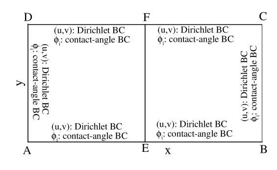
(a)

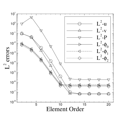
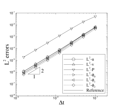
(b) (c)

Figure 1: Spatial/temporal convergence rates: (a) Problem configuration; (b) $L^{2}$ errors of flow variables versus element order (fixed $\Delta t=0.001$ and $t_{f}=0.1$); (c) $L^{2}$ errors of flow variables versus time step size $\Delta t$ (fixed element order $16$ and $t_{f}=1.0$).

The goal of this section is to demonstrate the spatial and temporal convergence rates of the method developed herein using a contrived analytic solution under non-trivial contact angles.

The setting of this problem is illustrated in Figure 1(a). We consider a rectangular domain $\overline{ABCD}$, $0\leqslant x\leqslant 2$ and $-1\leqslant y\leqslant 1$, and a four-fluid mixture (i.e. $N=4$) contained in this domain. Assume field distributions for the velocity, pressure and phase field functions given by the following expressions

$$\left\{\begin{split}&u=A_{0}\sin(ax)\cos(\pi y)\sin(\omega_{0}t)\\ &v=-(A_{0}a/\pi)\cos(ax)\sin(\pi y)\sin(\omega_{0}t)\\ &P=A_{0}\sin(ax)\sin(\pi y)\cos(\omega_{0}t)\\ &\phi_{1}=\frac{1}{6}\left[1+A_{1}\cos(a_{1}x)\cos(\bar{b}_{1}y)\sin(\omega_{1}t)\right]\\ &\phi_{2}=\frac{1}{6}\left[1+A_{2}\cos(a_{2}x)\cos(\bar{b}_{2}y)\sin(\omega_{2}t)\right]\\ &\phi_{3}=\frac{1}{6}\left[1+A_{3}\cos(a_{3}x)\cos(\bar{b}_{3}y)\sin(\omega_{3}t)\right],\\ \end{split}\right.$$ (131)

where ($u$, $v$) are the $x$ and $y$ components of the velocity $\mathbf{u}$. $A_{i}$, $\omega_{i}$ ($0\leqslant i\leqslant 3$), $a$, $a_{i}$ and $\bar{b}_{i}$ ($1\leqslant i\leqslant 3$) are constant parameters to be specified later. The above expressions for the velocity satisfy equation (4). We choose the $\mathbf{f}$ term in equation (109) such that the analytic expressions given in (131) satisfy equation (109). We choose the $g_{i}$ ($1\leqslant i\leqslant 3$) terms in equations (111) such that the expressions from (131) satisfy each of the ($N-1$) equations (111).

For the boundary conditions, we impose velocity Dirichlet condition (108) on all domain boundaries, where the boundary velocity $\mathbf{w}$ are chosen according to the velocity analytic expressions in (131). For the phase field variables we impose the contact-angle conditions (113)–(114) on the domain boundaries, where the source terms $g_{ai}$ and $g_{bi}$ ($1\leqslant i\leqslant 3$) are chosen such that the analytic expressions for $\phi_{i}$ from (131) satisfy the equations (113)–(114) on the boundaries with contact angles $(\theta_{14},\theta_{24},\theta_{34})=(120^{0},30^{0},135^{0})$. For the initial conditions, we choose the initial velocity and initial phase field distributions according to the analytic expressions of (131) by setting $t=0$.

Parameters	Values	Parameters	Values
$A_{0}$	$2.0$	$A_{1}$, $A_{2}$, $A_{3}$	$1.0$
$a$, $a_{1}$, $a_{2}$, $a_{3}$	$\pi$	$\bar{b}_{1}$, $\bar{b}_{2}$, $\bar{b}_{3}$	$\pi$
$\omega_{0}$, $\omega_{1}$	$1.0$	$\omega_{2}$	$1.2$
$\omega_{3}$	$0.8$	$\eta$	$0.1$
$\tilde{\rho}_{1}$	$1.0$	$\tilde{\rho}_{2}$	$3.0$
$\tilde{\rho}_{3}$	$2.0$	$\tilde{\rho}_{4}$	$4.0$
$\tilde{\mu}_{1}$	$0.01$	$\tilde{\mu}_{2}$	$0.02$
$\tilde{\mu}_{3}$	$0.03$	$\tilde{\mu}_{4}$	$0.04$
$\sigma_{12}$	$6.236E-3$	$\sigma_{13}$	$7.265E-3$
$\sigma_{14}$	$3.727E-3$	$\sigma_{23}$	$8.165E-3$
$\sigma_{24}$	$5.270E-3$	$\sigma_{34}$	$6.455E-3$
$\theta_{14}$	$120^{0}$	$\theta_{24}$	$30^{0}$
$\theta_{34}$	$135^{0}$	$m_{0}$	$1.0E-5$
$\rho_{0}$	$\min(\tilde{\rho}_{1},\dots,\tilde{\rho}_{4})$	$\nu_{0}$	$\max\left(\frac{\tilde{\mu}_{1}}{\tilde{\rho}_{1}},\dots,\frac{\tilde{\mu}_{4}}{\tilde{\rho}_{4}}\right)$
$J$ (temporal order)	$2$	$t_{f}$	$0.1$ or $1.0$
$\Delta t$	(varied)	Number of elements	$2$
Element order	(varied)

Table 2: Parameter values for the convergence-rate tests.

To simulate the problem we discretize the domain using two quadrilateral spectral elements of the same size, as shown in Figure 1(a). The volume fractions are chosen as the order parameters, as defined in (24). We integrate in time, from $t=0$ to $t=t_{f}$ ($t_{f}$ to be specified later), the governing equations for this four-phase system using the algorithm developed in Section 4. Then we compare the numerical solution and the exact solution given in (131) at $t=t_{f}$ to quantify the numerical errors for different flow variables. The values for the physical and numerical parameters of this problem are listed in Table 2.

Two group of tests have been performed. In the first group, we fix the integration time at $t_{f}=0.1$ and the time step size at $\Delta t=0.001$ ($100$ time steps), and vary the element order systematically between $2$ and $20$. The same element order has been used for all elements. Figure 1(b) plots the numerical errors at $t=t_{f}$ in $L^{2}$ norm for different flow variables as a function of the element order. It is evident that within a certain range of the element order (below about $12$) the errors decrease exponentially with increasing element order, exhibiting an exponential convergence rate in space. Beyond the element order of about $12$, the error curves level off as the element order further increases, exhibiting a saturation caused by the temporal truncation error.

In the second group of tests, we fix the integration time at $t_{f}=1.0$ and the element order at a large value $16$, and vary the time step size systematically between $\Delta t=0.0015625$ and $\Delta t=0.1$. Figure 1(c) shows the numerical errors at $t=t_{f}$ in $L^{2}$ norm for different variables as a function of $\Delta t$ in logarithmic scales. A reference line for a temporal second-order convergence rate has also been shown in the plot. It is evident that the numerical errors exhibit a second-order convergence rate in time.

The above results indicate that the method developed herein has a spatial exponential convergence rate and a temporal second-order convergence rate with multiple fluid components and different contact angles in the system.

5.2 Equilibrium Liquid Drops on Partially Wettable Wall – Comparison with de Gennes Theory

In this section we study the equilibrium configurations of two liquid drops – a water drop and an oil drop in ambient air – that are sufficiently far apart from each other, resting on a partially-wettable horizontal wall. This is a three-phase problem ($N=3$). However, because the two liquid drops are far apart, their interactions are weak, and the equilibrium shape of each drop will essentially be the same as the shape of that drop alone in the air. This allows us to compare qualitatively and quantitatively the numerical results of three-phase simulations on the contact angle effects with the de Gennes theory deGennesBQ2003 on the equilibrium drop shape for two-phase problems.

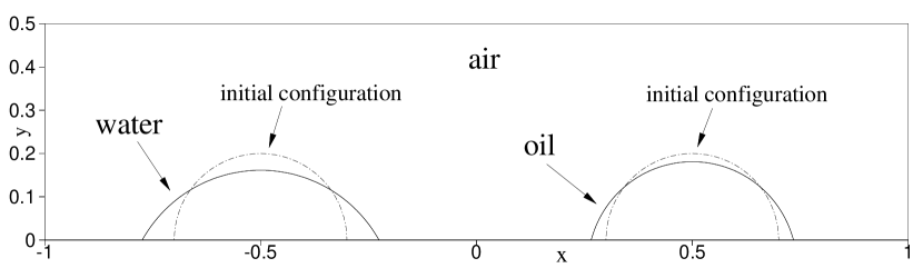
(a) (b)

Figure 2: Three-phase flows (zero gravity), equilibrium configurations of a water drop and an oil drop on a partially-wettable horizontal wall surface with contact angles: (a) $(\theta_{aw},\theta_{ao})=(60^{0},75^{0})$; (b) $(\theta_{aw},\theta_{ao})=(135^{0},75^{0})$. Solid curves denote the drop profiles from the simulations, visualized by the contour levels $c_{i}=\frac{1}{2}$ ($i=1,2,3$). In (a) the dashed-dot curves show the initial configurations (half circles) of the liquid drops. In (b) the dashed curves show the theoretical equilibrium drop profiles for the corresponding contact angles.

We consider a rectangular domain, $-L\leqslant x\leqslant L$ and $0\leqslant y\leqslant L/2$, where $L=4$cm; see Figure 2(a). The bottom and top sides of the domain are solid walls, with certain wettability properties. In the horizontal direction the domain is assumed to be periodic at $x=\pm L$. The domain is filled with air. Two liquid drops, a water drop and an oil drop, both initially semi-circular with a radius $R_{0}=L/5$, are held at rest on the bottom wall. Initially the center of the water drop is at $\mathbf{X}_{w}=(x_{0w},y_{0w})=(-L/2,0)$, and the center of the oil drop is at $\mathbf{X}_{o}=(x_{0o},y_{0o})=(L/2,0)$. The gravity is in the vertical direction, pointing downward. We use $\theta_{aw}$ and $\theta_{ao}$ to denote the static contact angles of the air-water interface and the air-oil interface on the wall, respectively. Note that these are the angles measured on the side of the liquid by convention. At $t=0$ the system is released and starts to evolve, eventually reaching an equilibrium state. Our goal is to study the equilibrium configuration of this three-phase system.

Density $[kg/m^{3}]$:	Air – $1.2041$	Water – $998.207$	Oil – $870$
Dynamic viscosity $[kg/(m\cdot s)]$:	Air – $1.78\times 10^{-4}$	Water – $1.002\times 10^{-3}$	Oil – $9.15\times 10^{-2}$
Surface tension $[kg/s^{2}]$:	Air/water – $0.0728$	Air/oil – $0.055$ (or varied)	Oil/water – $0.04$
Gravitational acceleration $[m/s^{2}]$:	$0$ or $9.8$ (or varied)

Table 3: Physical parameter values for the air/water/oil three-phase system.

The physical parameters for this problem include the densities and dynamic viscosities of the three fluids (air, water and oil), as well as the three pairwise surface tensions among them, together with the gravitational acceleration. The values for these parameters employed in this paper are listed in Table 3. We use $L$ as the length scale and the air density as the density scale $\varrho_{d}$, and choose the velocity scale as $U_{0}=\sqrt{g_{r0}L}$, where $g_{r0}=1m/s^{2}$. Then the problem is normalized based on Table 1.

In the simulations we assign the water, oil and air as the first, second, and third fluids, respectively. The two independent contact angles for this three-phase system are therefore $\theta_{13}$ (air-water contact angle $\theta_{aw}$) and $\theta_{23}$ (air-oil contact angle $\theta_{a}o$). We employ the volume fractions $c_{i}$ ($1\leqslant i\leqslant N-1$) as the order parameters; see equations (24) and (25).

To simulate this problem we partition the domain using $100$ quadrilateral spectral elements of the same size, with $20$ elements along the $x$ direction and $5$ elements along the $y$ direction. We employ an element order of $14$ within each element. On the top and bottom walls ($y=0,L/2$), we impose the Dirichlet condition (108) with $\mathbf{w}=0$ for the velocity, and the contact-angle boundary conditions (113)–(114) with $g_{ai}=0$ and $g_{bi}=0$ for the phase field variables $\phi_{i}$ ($1\leqslant i\leqslant N-1$). In the horizontal direction, periodic boundary conditions are imposed for all flow variables.

Parameters	Values
$\zeta_{ij}$	Computed based on (66) and (28)
$\eta/L$	$0.01$
$m_{0}/(U_{0}L^{3})$	$10^{-9}$
$\rho_{0}$	$\min(\tilde{\rho}_{1},\tilde{\rho}_{2},\tilde{\rho}_{3})$
$\nu_{0}$	$5\max\left(\frac{\tilde{\mu}_{1}}{\tilde{\rho}_{1}},\frac{\tilde{\mu}_{2}}{\tilde{\rho}_{2}},\frac{\tilde{\mu}_{3}}{\tilde{\rho}_{3}}\right)$
$S$	$\eta^{2}\sqrt{\frac{4\gamma_{0}}{m_{0}\Delta t}}$
$\alpha$	Computed based on (121)
$U_{0}\Delta t/L$	$2.0\times 10^{-6}$
$\theta_{13}$, $\theta_{23}$	ranging between $15^{0}$ and $165^{0}$
$J$ (temporal order)	$2$
Number of elements	$100$
Element order	$14$

Table 4: Simulation parameter values for air/water/oil three-phase problem.

The governing equations (109), (4), and (111) with $g_{i}=0$, together with the above boundary conditions are solved using the algorithm presented in Section 4. The initial velocity is set to $\mathbf{u}=0$, and the initial phase field distributions are set to

$$\left\{\begin{split}&\phi_{0}=\frac{1}{2}\left(1-\tanh\frac{|\mathbf{x}-\mathbf{X}_{w}|-R_{0}}{\sqrt{2}\eta}\right)\\ &\phi_{1}=\frac{1}{2}\left(1-\tanh\frac{|\mathbf{x}-\mathbf{X}_{o}|-R_{0}}{\sqrt{2}\eta}\right)\end{split}\right.$$ (132)

where $\mathbf{X}_{w}$ and $\mathbf{X}_{o}$ are the initial center coordinates of the water and oil drops, respectively. Table 4 summaries the values of the numerical parameters employed in the simulations.

(a) (b)

Figure 3: Three-phase flows (zero gravity): (a) Sketch of the equilibrium liquid-drop shape. (b) Comparison of the equilibrium drop height and spreading length as a function of the contact angle between the simulations and the de Gennes theory deGennesBQ2003 . Symbols include simulation results for both the water and oil drops. Multiple data points corresponding to a contact-angle value are results from different simulation cases with different $(\theta_{aw},\theta_{ao})$ combinations. For example, two combinations with $(\theta_{aw},\theta_{ao})=(60^{0},75^{0})$ and $(\theta_{aw},\theta_{ao})=(120^{0},60^{0})$ both contribute to the data for contact angle $60^{0}$.

5.2.1 Zero Gravity

We first focus on the case with no gravity, i.e. $g_{r}=0$, where $g_{r}$ denotes the magnitude of gravitational acceleration.

Since the two drops are sufficiently far apart on the wall, their influence on each other is small. In case of zero gravity the surface tensions are the only forces that come into play in the system. The equilibrium profile of each drop will be a circular cap (or a spherical cap in three dimensions), which intersects the wall surface at the prescribed contact angle deGennesBQ2003 .

In Figure 2 we show the equilibrium configurations of the system from the simulations corresponding to two sets of contact-angle values, $(\theta_{aw},\theta_{ao})=(60^{0},75^{0})$ for Figure 2(a) and $(\theta_{aw},\theta_{ao})=(135^{0},75^{0})$ for Figure 2(b). The solid curves correspond to the contour levels $c_{i}=\frac{1}{2}$ ($1\leqslant i\leqslant 3$). In Figure 2(a) the dashed-dot curves correspond to the initial profiles (semi-circular) of the water and oil drops. In Figure 2(b) we have also shown two dashed circles as references. The intersecting angles of these circles at the wall are exactly $135^{0}$ (in the water region) and $75^{0}$ (in the oil region). In addition, the caps formed between these dashed circles and the wall have exactly the same area as the initial semi-circular shapes of the water and oil drops (i.e. $\frac{1}{2}\pi R_{0}^{2}$). The water-drop and oil-drop profiles obtained from the simulations (solid curves) almost exactly overlap with those of the dashed circular caps in Figure 2(b). This indicates that the simulation has produced results that are qualitatively consistent with the theory deGennesBQ2003 .

To provide a quantitative comparison, we focus on the parameters spreading length $L_{s}$ and drop height $H_{d}$, as defined in Figure 3(a), of the equilibrium drop profile at zero gravity. Let $R$ denote the radius of the circle at equilibrium, and $\theta_{E}$ denote the contact angle. Then based on the volume conservation of the liquid drop we can obtain the following relations deGennesBQ2003 ; Dong2012 ,

$$\left\{\begin{split}&R=R_{0}\sqrt{\frac{\pi/2}{\theta_{E}-\sin\theta_{E}\cos\theta_{E}}}\\ &H_{d}=R(1-\cos\theta_{E})\\ &L_{s}=2R\sin\theta_{E},\end{split}\right.$$ (133)

where the initial drop profile is assumed to be semi-circular with a radius $R_{0}$. These theoretical expressions for the equilibrium drop parameters allow for quantitative comparisons with numerical simulations.

We have performed a series of numerical simulations of this three-phase problem with various combinations for the contact angles $(\theta_{aw},\theta_{ao})$, in particular, with a fixed $\theta_{aw}=120^{0}$ and $\theta_{ao}$ varied systematically between $15^{0}$ and $165^{0}$, and with a fixed $\theta_{ao}=75^{0}$ and $\theta_{aw}$ varied systematically between $15^{0}$ and $165^{0}$. For each pair of contact angles $(\theta_{aw},\theta_{ao})$, we have conducted simulations of this three-phase problem, and obtained the spreading length and the drop height from the equilibrium profiles of the water and oil drops. In Figure 3(b) we plot the spreading length and the drop height (symbols) as a function of the contact angle for both the water and the oil drops. For comparison we have also included in this plot the theoretical relations given by (133) (see the solid/dashed curves). Note that at zero gravity the theoretical relations (133) apply to both water and oil drops. Accordingly, we have not differentiated the water and oil drops when plotting the numerical results in Figure 3(b), and the symbols represent results for both the water drops and the oil drops from the simulations. We observe that the numerical results for the equilibrium drop height are in good agreement with the theoretical results for the whole range of contact-angle values ($[15^{0},165^{0}]$) consider here. For the spreading length, the numerical results also agree quite well with the theoretical results in the bulk range of contact angles ($[30^{0},150^{0}]$). However, at very small (or very large) contact angles (e.g. $15^{0}$ and $165^{0}$) we observe a larger discrepancy between the numerically obtained values and the theoretical values for the spreading length.

The results of this subsection indicate that our simulation results compare favorably with the de Gennes theory deGennesBQ2003 both qualitatively and quantitatively at zero gravity with multiple fluid components and multiple types of contact angles.

5.2.2 Effects of Gravity and Surface Tension

In this subsection we consider how the gravity influences the equilibrium profiles of the water and oil drops. We will also look into the effect of surface tensions on the system.

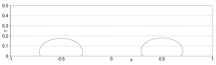
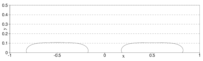
(a) (b) (c)

Figure 4: Three-phase flows, effect of gravity on equilibrium profiles of water/oil drops with contact angles $(\theta_{aw},\theta_{ao})=(120^{0},135^{0})$: (a) zero gravity, (b) gravity $g_{r}=3m/s^{2}$, (c) gravity $g_{r}=12m/s^{2}$.

In the presence of gravity, the equilibrium profile of the liquid drop is determined by the balance of three effects. These effects are associated with (i) the gravity, which tends to spread the drop on the wall; (ii) the surface tension, which tends to restore the drop to a circular cap; (iii) the contact angle, which the drop profile must respect at the wall. More specifically, one can define a capillary length associated with the liquid-air interface deGennesBQ2003 , $\kappa^{-1}=\sqrt{\frac{\sigma_{la}}{\rho_{l}g_{r}}}$, where $\sigma_{la}$ is the surface tension associated with the interface, $\rho_{l}$ is the liquid density and $g_{r}$ is the magnitude of the gravitational acceleration. If the drop size is much smaller than $\kappa^{-1}$, then the surface tension is dominant and the liquid drop forms a circular cap at equilibrium. If the drop size is much larger than $\kappa^{-1}$, then the gravity is dominant and the drop forms a puddle (or pancake-like shape) at equilibrium, with a flat liquid surface deGennesBQ2003 . Moreover, if the gravity is dominant (liquid forming a puddle), by considering the force and the Young’s relation one can obtain the following expression for the puddle thickness (height) in terms of other physical parameters (see deGennesBQ2003 )

$$H_{\infty}=2\kappa^{-1}\sin\left(\frac{\theta_{E}}{2}\right)=2\sqrt{\frac{\sigma_{la}}{\rho_{l}g_{r}}}\sin\left(\frac{\theta_{E}}{2}\right)$$ (134)

where $H_{\infty}$ denotes the asymptotic puddle thickness, and $\theta_{E}$ is the equilibrium contact angle at the wall.

We have performed two groups of numerical experiments to study the effects of the gravity and the surface tension, respectively.

In the first group of experiments, we fix all the other physical parameters at those values given in Table 3 (air-oil surface tension is fixed at $0.055kg/s^{2}$), and vary only the magnitude of the gravitational acceleration $g_{r}$ systematically. We have conducted a series of simulations of this three-phase system corresponding to these gravity values. Figure 4 shows the equilibrium profiles of the water and oil drops corresponding to three gravity values. The drop profiles again are visualized by the volume-fraction contour levels $c_{i}=\frac{1}{2}$ ($1\leqslant i\leqslant 3$). These results are for an air-water contact angle of $120^{0}$ and an air-oil contact angle of $135^{0}$. With zero gravity, the drops form circular caps (Figure 4(a)). With a large gravity $g_{r}=12m/s^{2}$, both drops form a puddle on the wall, with a flattened top surface (Figure 4(c)). With an intermediate gravity magnitude $g_{r}=3m/s^{2}$, the drops form oval caps (or elongated circular caps) on the wall (Figure 4(b)). These observations are consistent with the theory of deGennesBQ2003 .

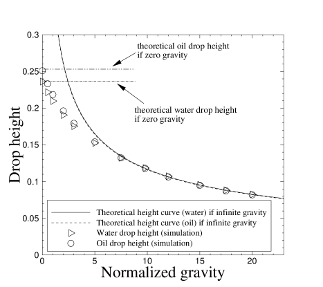
Figure 5: Effect of gravity: equilibrium water/oil drop heights as a function of gravity, with contact angles $(\theta_{aw},\theta_{ao})=(120^{0},135^{0})$. Solid/dashed curves show the theoretical asymptotic drop-height curves if gravity is dominant. The theoretical water/oil drop heights at zero gravity are also marked in the figure.

We have computed the heights of the water/oil drops from their equilibrium profiles corresponding to each gravity value. In Figure 5 we plot the heights of the water drop and the oil drop as a function of the gravity obtained from our simulations (see the symbols) corresponding to a set of fixed contact angles $(\theta_{aw},\theta_{ao})=(120^{0},135^{0})$. For comparison we have included in this plot the theoretical drop-height (puddle thickness) for water and for oil if the gravity is dominant, computed based on equation (134), as a function of the gravity for the same set of contact angles; see the solid and dashed curves. Note that these theoretical height curves are valid only for sufficiently large gravity values. They are invalid if the gravity is small. In addition, we have also included in this figure the theoretical heights for the water drop and the oil drop at zero gravity for $(\theta_{aw},\theta_{ao})=(120^{0},135^{0})$, which are computed based on equation (133). It can be observed that the drop-height values from numerical simulations agree with the theoretical values very well when the gravity becomes large (beyond about $7.5kg/m^{2}$). At zero gravity the simulation results are also in good agreement with the theoretical results. For intermediate gravity values, the simulation results exhibit a transition between the results of these two extreme cases.

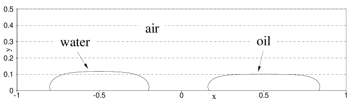
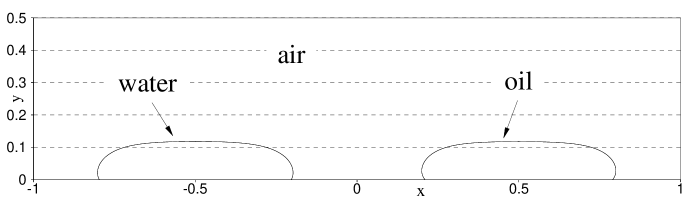
(a) (b)

Figure 6: Three-phase flows, effect of air-oil surface tension on equilibrium drop profiles: (a) $\sigma_{ao}=0.04kg/s^{2}$, (b) $\sigma_{ao}=0.055kg/s^{2}$. Contact angles are $(\theta_{aw},\theta_{ao})=(120^{0},135^{0})$. All other physical parameters are fixed.

In the second group of experiments we investigate the effect of the surface tension on the liquid drop heights when the gravity is dominant (i.e. liquid forming a puddle). In these tests we vary the air-oil surface tension systematically over a range of values while fixing all the other physical parameters. We use the normal gravitational acceleration $g_{r}=9.8m/s^{2}$, and the air-water and air-oil contact angles are fixed at $(\theta_{aw},\theta_{ao})=(120^{0},135^{0})$. The values for the rest of the physical parameters (excluding the air-oil surface tension) are given in Table 3. Figure 6 shows the equilibrium configurations of this three-phase system corresponding to two air-oil surface tensions $\sigma_{ao}=0.04kg/s^{2}$ and $0.055kg/s^{2}$. One can observe that both the water and oil drops form a puddle on the wall in this case, and the thickness of the oil puddle is notably influenced by the air-oil surface tension. We have computed the oil-puddle thickness from the equilibrium configurations corresponding to each air-oil surface tension value. In Figure 7 we compare the oil-puddle thickness squared as a function of the air-oil surface tension between the simulations and the de-Gennes theory (see equation (134)). The simulation results agree quite well with the theoretical relation.

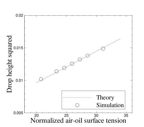
Figure 7: Three-phase flows, comparison of the oil-puddle thickness squared as a function of the normalized air/oil surface tension between simulation and the de Gennes theory. Contact angles are fixed at $(\theta_{aw},\theta_{ao})=(120^{0},135^{0})$.

The results of this section and the comparisons with the de Gennes theory deGennesBQ2003 indicate that, for multiphase problems involving solid walls and multiple types of fluid interfaces and contact angles, the method developed herein produces physically accurate results.

5.3 Compound Drops of Multiple Fluids on Horizontal Wall Surfaces – Effect of Contact Angles

We study the equilibrium configurations of compound drops formed by multiple fluids on a wall surface in this section, and how the various contact angles influence the drop configurations. Two multiphase systems will be considered, consisting of three and four fluid components, respectively. Because the interactions among the fluids are strong, in certain cases the profile of the compound drop can be dramatically modified with a small change in the contact angles.

5.3.1 Three Fluid Components

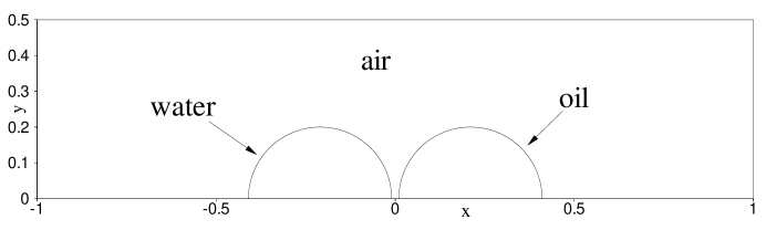
Figure 8: Compound liquid drop: initial profiles of water and oil drops.

First let us consider a three-phase flow problem consisting of air, water and oil, with a setting similar to that of Section 5.2, More specifically, we consider the rectangular domain as shown in Figure 8, $-L\leqslant x\leqslant L$ and $0\leqslant y\leqslant 0.5L$ ($L=4cm$), where the top and bottom are solid walls and in the horizontal direction it is periodic. A water drop and an oil drop, both semi-circular initially with radius $R_{0}=0.2L$, are in ambient air and held at rest on the bottom wall. The two drops are placed next to and almost touching each other. The water-drop center is located at $\mathbf{X}_{w}=(x_{0w},y_{0w})=(-0.21L,0)$, and the oil-drop center is at $\mathbf{X}_{o}=(x_{0o},y_{0o})=(0.21L,0)$. The gravity is in the $-y$ direction. Let $\theta_{aw}$ denote the contact angle between the air-water interface and the wall when measured on the water side, and $\theta_{ao}$ denote the contact angle between the air-oil interface and the wall when measured on the oil side. At $t=0$ the system is released, and evolves to equilibrium eventually. Because the two liquid drops are very close to each other, they merge and form a compound drop on the wall. Our goal is to study how the profile of the compound drop at equilibrium is affected by the wall wettability, i.e. the contact angles $\theta_{aw}$ and $\theta_{ao}$.

In the present simulations we employ the values listed in Table 3 for the physical parameters about the air, water and oil and the interfaces formed by these fluids. Water, oil and air are assigned as the first, second and third fluids, respectively. Similar to in Section 5.2, the problem is normalized by choosing $L$ as the length scale, the air density as the density scale ${\varrho}_{d}$, and $\sqrt{g_{r0}L}$ (where $g_{r0}=1m/s^{2}$) as the velocity scale $U_{0}$.

Parameters	Values
$\phi_{i}$	defined by (24), volume fractions as order parameters
$\zeta_{ij}$	Computed based on (66) and (28)
$\eta/L$	$0.01$
$m_{0}/(U_{0}L^{3})$	$10^{-7}$
$\rho_{0}$	$\min(\tilde{\rho}_{1},\tilde{\rho}_{2},\tilde{\rho}_{3})$
$\nu_{0}$	$5\max\left(\frac{\tilde{\mu}_{1}}{\tilde{\rho}_{1}},\frac{\tilde{\mu}_{2}}{\tilde{\rho}_{2}},\frac{\tilde{\mu}_{3}}{\tilde{\rho}_{3}}\right)$
$S$	$\eta^{2}\sqrt{\frac{4\gamma_{0}}{m_{0}\Delta t}}$
$\alpha$	Computed based on (121)
$U_{0}\Delta t/L$	$2.0\times 10^{-6}$
$\theta_{13}$, $\theta_{23}$	ranging between $45^{0}$ and $135^{0}$
$J$ (temporal order)	$2$
Number of elements	$100$
Element order	$14$

Table 5: Simulation parameter values for air/water/oil three-phase problem.

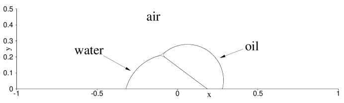
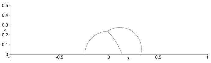
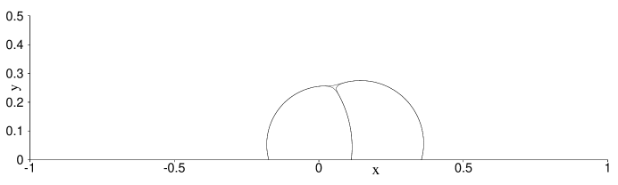
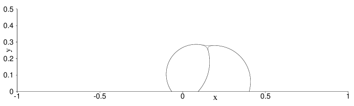
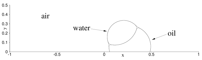
(a) (b) (c) (d) (e)

Figure 9: Profiles of the compound liquid drop formed by water and oil, with the air/oil contact angle fixed at $\theta_{ao}=105^{0}$ and the air/water contact angle varied: (a) $\theta_{aw}=75^{0}$, (b) $\theta_{aw}=90^{0}$, (c) $\theta_{aw}=105^{0}$, (d) $\theta_{aw}=125^{0}$, (e) $\theta_{aw}=135^{0}$.

The domain is partitioned using $100$ spectral elements (with $20$ and $5$ elements in the $x$ and $y$ directions, respectively), and an element order $14$ is employed in the simulations. On the top and bottom walls, no slip condition is imposed for the velocity, and for the phase field functions the contact-angle conditions (113)–(114) are imposed with $g_{ai}=0$ and $g_{bi}=0$. Periodic conditions are imposed for all flow variables in the horizontal direction. The initial velocity is assumed to be zero, and the initial distributions of the phase field functions are given by the expressions (132) by noting that $x_{0w}=-0.21L$ and $x_{0o}=0.21L$ in this case. Table 5 lists the simulation parameters employed for this test problem.

We observe that the wettability of the wall, i.e. the contact angles of the various fluids forming the compound drop, can considerably affect the equilibrium configurations of the drop. To demonstrate this point, let us assume that the gravity is absent, and the system is influenced only by the surface tensions among the air, water and oil. The results shown in Figure 9 demonstrate the effect of the air-water contact angle on the equilibrium shape of the water/oil compound drops. Plotted here are the profiles of the fluid interfaces, visualized by the contour levels of the volume fractions $c_{i}(\vec{\phi})=\frac{1}{2}$ ($1\leqslant i\leqslant 3$) for the three fluids. In this group of tests, the contact angle of the air-oil interface has been fixed at $\theta_{ao}=105^{0}$, while the contact angle of the air-water interface $\theta_{aw}$ is varied in a range of values, from $75^{0}$ to $135^{0}$. Around the three-phase line where the three fluid components intersect a small star-shaped region can be observed. As pointed out in Dong2014 ; Dong2015 , such a region is formed by the contour levels because no fluid has a volume fraction larger than $\frac{1}{2}$ in that region. We can observe that the water and oil form a compound drop. The contact angle of the water-oil interface and the overall profile of the compound drop are affected by the air-water contact angle remarkably. With air-water contact angle $\theta_{aw}=75^{0}$ the water partially goes underneath the oil at equilibrium (Figure 9), with the contact angle of the water-oil interface (measured on the water side) being about $\theta_{ow}\approx 34^{0}$ according to equation (90). As the air-water contact angle increases the contact angle of the water-oil interface increases more rapidly, and the region occupied by the water becomes more “plump” within the compound drop (Figures 9(b)-(d)). Based on equation (90), as the air-water contact angle increases to about $\theta_{aw}=138.16^{0}$ the water-oil contact angle will reach $\theta_{ow}=180^{0}$. In practice we have observed from numerical experiments that, when the air-water contact angle is below but close to this value, the water tends to move away from the wall at equilibrium because of the large contact angle of the water-oil interface. For example, with an air-water contact angle $\theta_{aw}=135^{0}$ the water forms a drop on the shoulder of the oil region, and the water drop is not in contact with the wall any more under current simulation conditions; see Figure 9(e).

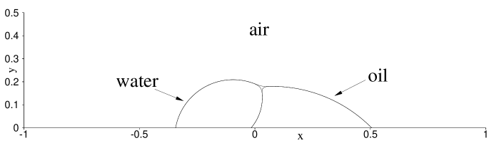
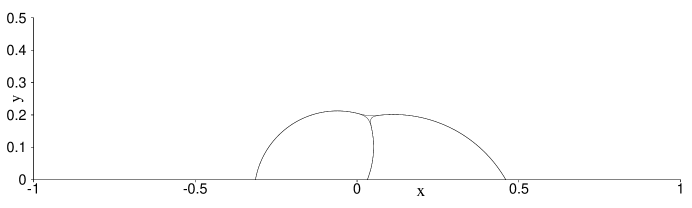
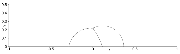
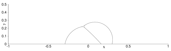
(a) (b) (c) (d)

Figure 10: Profiles of the compound liquid drop formed by water and oil, with the air/water contact angle fixed at $\theta_{aw}=80^{0}$ and the air/oil contact angle varied: (a) $\theta_{ao}=45^{0}$, (b) $\theta_{ao}=60^{0}$, (c) $\theta_{ao}=90^{0}$, (d) $\theta_{ao}=105^{0}$.

Figure 10 shows the equilibrium configurations of the compound water-oil drop corresponding to several values of the air-oil contact angle. In this group of tests the air-water contact angle is fixed at $\theta_{aw}=80^{0}$, and the air-oil contact angle is varied in a range of values between $\theta_{ao}=45^{0}$ and $\theta_{ao}=105^{0}$. According to equation (90), the contact angle of the water-oil interface (measured on the water side) varies between $\theta_{ow}\approx 131^{0}$ (Figure 10(a)) and $\theta_{ow}\approx 48^{0}$ (Figure 10(d)). It is evident that the overall profile of the compound drop, and the profiles of the water and oil regions within the drop, have been dramatically influenced by the change in the air-oil contact angle.

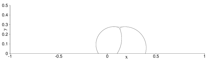
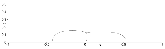
(a) (b) (c)

Figure 11: Effect of gravity on profiles of compound liquid drop formed by water and oil with contact angles $(\theta_{aw},\theta_{ao})=(120^{0},105^{0})$: (a) zero gravity, (b) $g_{r}=2m/s^{2}$, (c) $g_{r}=5m/s^{2}$.

It is also observed that the gravity can affect the equilibrium configuration of the compound drop significantly. Figure 11 shows the equilibrium configurations of the compound drop of water and oil corresponding to three values of the gravitational acceleration: $g_{r}=0$, $2m/s^{2}$ and $5m/s^{2}$. These results correspond to the air-water and air-oil contact angles $(\theta_{aw},\theta_{ao})=(120^{0},105^{0})$. The increase in the gravity tends to spread the compound drop onto the wall, reducing the drop height. The drop becomes very stretched along the horizontal direction at large gravity values.

5.3.2 Four Fluid Components

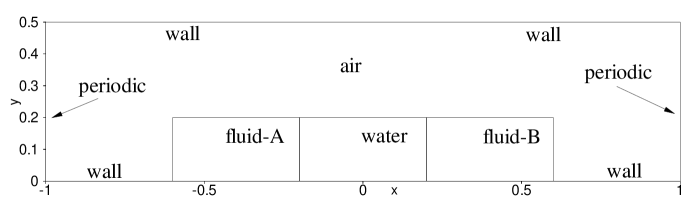
Figure 12: Initial configuration of a compound liquid drop consisting of water, fluid-A and fluid-B (in ambient air) on a horizontal wall.

We next study a four-phase problem, and consider a compound liquid drop consisting of three liquids (in ambient air) on a solid wall surface. We will look into the effects of various contact angles. The multitude of independent contact angles much complicates the interactions among different fluids.

Specifically, we consider the problem as sketched in Figure 12. A rectangular domain, of dimensions $-L\leqslant x\leqslant L$ and $0\leqslant y\leqslant L/2$ (where $L=4cm$) and with solid walls on the top and bottom sides, is filled with air and contains three liquids (water, fluid-A and fluid-B) within. The initial region occupied by these liquids are shown in Figure 12. The three liquid regions all have an initial height $0.2L$ (i.e. $0\leqslant y\leqslant 0.2L$). In the horizontal direction water occupies the region $-0.2L\leqslant x\leqslant 0.2L$, fluid-A occupies $-0.6L\leqslant x\leqslant-0.2L$, and fluid-B occupies $0.2L\leqslant x\leqslant 0.6L$. All these fluids are assumed to be incompressible and immiscible with one another. In the horizontal direction the domain is assumed to be periodic at $x=\pm L$. The gravity is ignored for this problem. All the four fluids are held at rest initially. Then at $t=0$ the system is released and starts to evolve under the six pairwise surface tensions among these fluids, eventually reaching an equilibrium configuration. Our goal is to investigate the effects of various contact angles on the equilibrium configuration of this system. We employ the physical parameter values as listed in Table 6 for this problem.

density [$kg/m^{3}$]:	air – $1.2041$, water – $998.207$, fluid-A – $870$, fluid-B – $400$
dynamic viscosity [$kg/m\cdot s$]:	air – $1.78E-4$, water – $1.002E-3$, fluid-A – $0.0915$, fluid-B – $0.02$
surface tension [$kg/s^{2}$]:	air/water – $0.0728$, air/fluid-A – $0.055$, air/fluid-B – $0.06$,
	water/fluid-A – $0.044$, water/fluid-B – $0.045$, fluid-A/fluid-B – $0.048$

Table 6: Physical parameter values for the four-phase flow problem with air, water, fluid-A and fluid-B.

We assign the water, fluid-A, fluid-B and air as the first, second, third and fourth fluids respectively in the simulations. Therefore the contact angles of the air-water interface ($\theta_{aw}$), the air/fluid-A interface ($\theta_{aA}$) and the air/fluid-B interface ($\theta_{aB}$) are chosen as the independent contact angles of this four-phase system. The normalization proceeds according to Table 1 by choosing $L$ as the length scale, the air density as the density scale $\varrho_{d}$, and $\sqrt{g_{r0}L}$ (where $g_{r0}=1m/s^{2}$) as the velocity scale $U_{0}$. We employ the volume fractions as the order parameters in this problem; see equations (24) and (25).

To simulate the problem we discretize the domain using $256$ quadrilateral spectral elements, with $32$ and $8$ elements along the $x$ and $y$ directions respectively. We use an element order $12$ for each element in the simulations. On the top and bottom walls we impose the Dirichlet boundary condition (108) with $\mathbf{w}=0$ for the velocity, and the contact-angle boundary conditions (113)–(114) with $g_{ai}=0$ and $g_{bi}=0$ for the phase field functions. Periodic conditions are imposed for all the flow variables in the horizontal direction. The initial velocity is zero. The initial phase field distributions are given by,

$$\left\{\begin{split}&\phi_{10}=\frac{1}{8}\left(1+\tanh\frac{x+0.2L}{\sqrt{2}\eta}\right)\left(1-\tanh\frac{x-0.2L}{\sqrt{2}\eta}\right)\left(1-\tanh\frac{y-0.2L}{\sqrt{2}\eta}\right)\\ &\phi_{20}=\frac{1}{8}\left(1+\tanh\frac{x+0.6L}{\sqrt{2}\eta}\right)\left(1-\tanh\frac{x+0.2L}{\sqrt{2}\eta}\right)\left(1-\tanh\frac{y-0.2L}{\sqrt{2}\eta}\right)\\ &\phi_{30}=\frac{1}{8}\left(1+\tanh\frac{x-0.2L}{\sqrt{2}\eta}\right)\left(1-\tanh\frac{x-0.6L}{\sqrt{2}\eta}\right)\left(1-\tanh\frac{y-0.2L}{\sqrt{2}\eta}\right)\\ &\phi_{40}=1-\phi_{10}-\phi_{20}-\phi_{30}.\end{split}\right.$$ (135)

Table 7 lists the values of the simulation parameters for this problem.

Parameters	Values
$\phi_{i}$	defined by (24)
$\zeta_{ij}$	Computed based on (66) and (28)
$\eta/L$	$0.01$
$m_{0}/(U_{0}L^{3})$	$10^{-9}$
$\rho_{0}$	$\min(\tilde{\rho}_{1},\tilde{\rho}_{2},\tilde{\rho}_{3})$
$\nu_{0}$	$5\max\left(\frac{\tilde{\mu}_{1}}{\tilde{\rho}_{1}},\frac{\tilde{\mu}_{2}}{\tilde{\rho}_{2}},\frac{\tilde{\mu}_{3}}{\tilde{\rho}_{3}}\right)$
$S$	$\eta^{2}\sqrt{\frac{4\gamma_{0}}{m_{0}\Delta t}}$
$\alpha$	Computed based on (121)
$U_{0}\Delta t/L$	$2.5\times 10^{-6}$
$\theta_{14}$, $\theta_{24}$, $\theta_{34}$	ranging between $60^{0}$ and $120^{0}$
$J$ (temporal order)	$2$
Number of elements	$256$
Element order	$12$

Table 7: Simulation parameter values for the four-phase air/water/fluid-A/fluid-B problem.

(a) (b) (c) (d)

Figure 13: Profiles of a compound liquid drop formed by water, fluid-A and fluid-B (ambient air) on a wall, with air/fluid-A and air/water contact angles fixed at $\theta_{aA}=\theta_{aw}=90^{0}$ and the air/fluid-B contact angle varied as: (a) $\theta_{aB}=60^{0}$, (b) $\theta_{aB}=80^{0}$, (c) $\theta_{aB}=100^{0}$, (d) $\theta_{aB}=120^{0}$.

Let us first look into the effect of the air/fluid-B contact angle on the equilibrium configuration of the system. In this set of tests we fix the contact angles of the air/water interface and the air/fluid-A interface at $\theta_{aw}=\theta_{aA}=90^{0}$, and vary the air/fluid-B contact angle in a range of values. Figure (13) shows the configurations of this system corresponding to four air/fluid-B contact angles: $\theta_{aB}=60^{0}$, $80^{0}$, $100^{0}$ and $120^{0}$. The profiles of the fluid regions are visualized by the volume-fraction contour levels $c_{i}=\frac{1}{2}$ ($1\leqslant i\leqslant 4$). One can observe that the change in the air/fluid-B contact angle not only impacts the fluid-B region, but also significantly affects the water region. Let $\theta_{wA}$ denote the contact angle of the water/fluid-A interface measured on the water side, and $\theta_{wB}$ denote the contact angle of the water/fluid-B interface measured on the water side. Then according to equation (90) $\theta_{wA}=90^{0}$ under the current conditions. On the other hand, as the $\theta_{aB}$ varies between $60^{0}$ and $120^{0}$, the water/fluid-B contact angle changes between $\theta_{wB}\approx 132^{0}$ and $\theta_{wB}\approx 48^{0}$ according to equation (90). The results shown in Figures 13(a)–(d) are qualitatively consistent with these theoretical results.

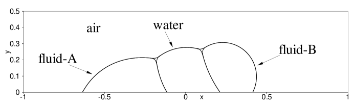
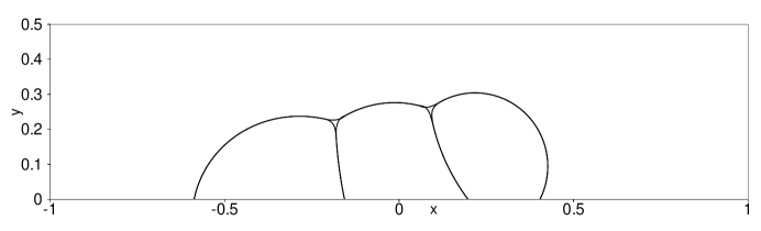
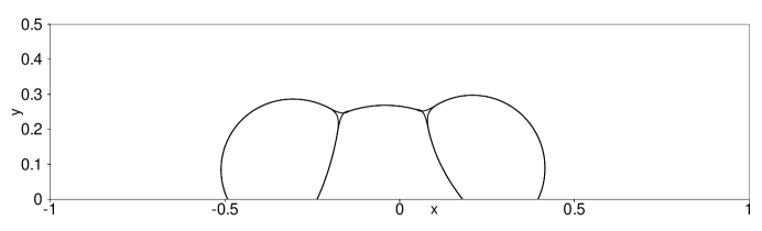
(a) (b) (c)

Figure 14: Profiles of a compound liquid drop formed by water, fluid-A and fluid-B (ambient air) on a wall, with air/water and air/fluid-B contact angles fixed at $\theta_{aw}=90^{0}$ and $\theta_{aB}=120^{0}$ and the air/fluid-A contact angle varied as: (a) $\theta_{aA}=60^{0}$, (b) $\theta_{aB}=80^{0}$, (c) $\theta_{aB}=120^{0}$.

Figure 14 demonstrates the effect of the air/fluid-A contact angle on the equilibrium configuration of the system. In this set of tests the air/water contact angle is fixed at $\theta_{aw}=90^{0}$ and the air/fluid-B contact angle is fixed at $\theta_{aB}=120^{0}$, while the air/fluid-A contact angle $\theta_{aA}$ is varied in a range of values. The variation in $\theta_{aA}$ alters the profiles of the fluid-A region and the water region noticeably, while the fluid-B region seems little affected. As $\theta_{aA}$ increases from $60^{0}$ to $120^{0}$ the region occupied by the fluid-A becomes more compact, and the water/fluid-A contact angle is varied between $\theta_{wA}\approx 129^{0}$ and $\theta_{wA}\approx 51^{0}$ according to equation (90). Note that the water/fluid-B contact angle is $\theta_{wB}\approx 48^{0}$ based on (90) under the current conditions.

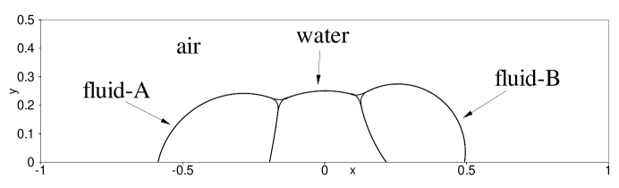
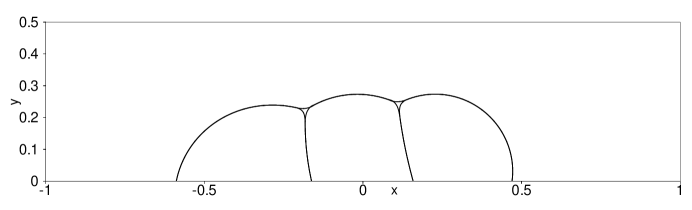
(a) (b) (c)

Figure 15: Profiles of a compound liquid drop formed by water, fluid-A and fluid-B (ambient air) on a wall, with air/fluid-A and air/fluid-B contact angles fixed at $\theta_{aA}=80^{0}$ and $\theta_{aB}=100^{0}$ and the air/water contact angle varied as: (a) $\theta_{aw}=75^{0}$, (b) $\theta_{aw}=90^{0}$, (c) $\theta_{aw}=105^{0}$.

Figure 15 demonstrates the effect of the air-water contact angle $\theta_{aw}$ on the configuration of the compound drop. In this group of tests the air/fluid-A and air/fluid-B contact angles are fixed at $\theta_{aA}=80^{0}$ and $\theta_{aB}=100^{0}$ respectively, and the air/water contact angle is varied. Note that even though the air/water interface is not in direct contact with the wall in this problem, the air/water contact angle $\theta_{aw}$ influences the contact angles of the other fluid interfaces in the system because of the Young’s relation (89). The profiles of the regions occupied by the water, fluid-A and fluid-B have all been modified by the variation in the air/water contact angle. The water region appears to become more rounded with increasing air/water contact angle. As the air/water contact angle increases from $\theta_{aw}=75^{0}$ to $\theta_{aw}=105^{0}$, the water/fluid-A contact angle (measured on the water side) increases from $\theta_{wA}\approx 78^{0}$ to $\theta_{wA}\approx 130^{0}$ according to (90), and the water/fluid-B contact angle (measured on the water side) increases from $\theta_{wB}\approx 49^{0}$ to $\theta_{wB}\approx 101^{0}$. The results in Figure 15 are qualitatively consistent with these theoretical predictions.

5.4 Impact of Liquid Drops on Partially Wettable Walls

The goal of this section is to demonstrate the performance of the method developed herein for studying the dynamics of multiphase flows involving the wall wettability. We will consider the impact of a water drop and an oil drop on a partially wettable horizontal wall.

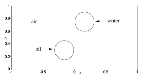
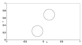
(a) (b) (c)

(d) (e) (f)

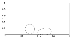
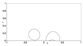
(g) (h) (i)

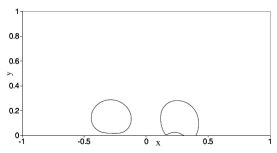
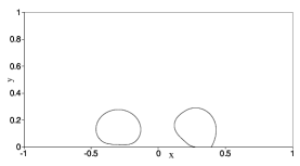
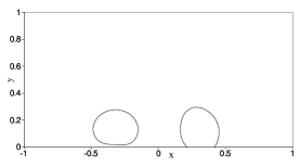
(j) (k) (l)

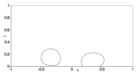
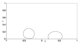
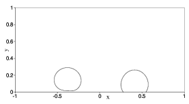
(m) (n) (o)

Figure 16: Impact of water/oil drops on horizontal wall with contact angles ($\theta_{ao},\theta_{aw})=(120^{0},120^{0})$: temporal sequence of snapshots of drop profiles at time instants (a) $t=0.0125$, (b) $t=0.1125$, (c) $t=0.175$, (d) $t=0.225$, (e) $t=0.2875$, (f) $t=0.3375$, (g) $t=0.375$, (h) $t=0.4375$, (i) $t=0.4625$, (j) $t=0.5$, (k) $t=0.525$, (l) $t=0.5625$, (m) $t=0.625$, (n) $t=0.6875$, (o) $t=0.75$.

More specifically, the problem configuration is illustrated in Figure 16(a). We consider a rectangular domain of dimensions $-L\leqslant x\leqslant L$ and $0\leqslant y\leqslant L$, where $L=8mm$. The top and bottom of the domain are two solid walls. In the horizontal direction the domain is periodic at $x=\pm L$. The domain is filled with air. A drop of wall and a drop of oil, both initially circular with a radius $R_{0}=0.15L$, are suspended in the air and held at rest. The center of the water drop is located at $\mathbf{X}_{w}=(x_{w},y_{w})=(0.16L,0.75L)$, and the oil-drop center is located at $\mathbf{X}_{o}=(x_{o},y_{o})=(-0.16L,0.3L)$. The gravity is assumed to be in the $-y$ direction. At $t=0$, the system is released, and the water and oil drops fall through the air. The oil drop impacts the wall first, followed by the water drop. Let $\theta_{aw}$ denote the contact angle between the air-water interface and the wall (measured on the water side), and $\theta_{ao}$ denote the contact angle between the air-oil interface and the wall (measured on the oil side). We look into the effect of the wall wettability on the dynamic behavior of this three-phase system.

We use the values listed in Table 3 for the physical parameters of air, water and oil in this problem. The gravitational acceleration is $9.8m/s^{2}$ in this problem. We take $L$ as the length scale, $U_{0}=\sqrt{g_{r0}L}$ (where $g_{r0}=1m/s^{2}$) as the velocity scale, and the air density as the density scale $\varrho_{d}$. The variables and parameters are then normalized according to Table 1. We assign water, oil and air as the first, second, and third fluids, respectively. The formulation with the volume fractions $c_{i}$ ($1\leqslant i\leqslant N-1$) as the order parameters is employed in the simulations.

Parameters	Values
$\phi_{i}$	defined by (24), volume fractions as order parameters
$\zeta_{ij}$	Computed based on (66) and (28)
$\eta/L$	$0.01$
$m_{0}/(U_{0}L^{3})$	$10^{-8}$
$\rho_{0}$	$\min(\tilde{\rho}_{1},\tilde{\rho}_{2},\tilde{\rho}_{3})$
$\nu_{0}$	$2\max\left(\frac{\tilde{\mu}_{1}}{\tilde{\rho}_{1}},\frac{\tilde{\mu}_{2}}{\tilde{\rho}_{2}},\frac{\tilde{\mu}_{3}}{\tilde{\rho}_{3}}\right)$
$S$	$\eta^{2}\sqrt{\frac{4\gamma_{0}}{m_{0}\Delta t}}$
$\alpha$	Computed based on (121)
$U_{0}\Delta t/L$	$2.5\times 10^{-6}$
$\theta_{13}$ ($\theta_{aw}$)	$120^{0}$, $150^{0}$
$\theta_{23}$ ($\theta_{ao}$)	$120^{0}$
$J$ (temporal order)	$2$
Number of elements	$512$
Element order	$12$

Table 8: Simulation parameter values for the dynamic problem of water and oil drops impacting the wall.

In order to simulate the problem, we discretize the domain using $512$ equal-sized quadrilateral spectral elements, with $32$ elements in the $x$ direction and $16$ elements in the $y$ direction. An element order $12$ is employed for each element in the simulations. On the top and bottom walls we impose the Dirichlet condition (108) with $\mathbf{w}=0$ for the velocity, and the contac-angle conditions (113)–(114) with $g_{ai}=0$ and $g_{bi}=0$ for the phase field variables. On the horizontal boundaries $x=\pm L$ periodic conditions are imposed on all the flow variables. The initial velocity is set to $\mathbf{u}=0$. Ihe initial phase field distributions are given by equation (132), in which the drop coordinates and radii are replaced by values for this problem. Table 8 lists the values of simulation parameters for this problem.

We have considered two sets of contact angles to demonstrate the effect of the wall wettability on the dynamics of the system. The air-oil contact angle is $\theta_{ao}=120^{0}$ in both sets, while the air-water contact angle is $\theta_{aw}=120^{0}$ in one set and $\theta_{aw}=150^{0}$ in the other.

We first look into the dynamic behavior of the liquid drops for the set of contact angles $(\theta_{aw},\theta_{ao})=(120^{0},120^{0})$. Figure 16 is a temporal sequence of snapshots of the fluid interfaces of this system, visualized by the contours of volume fractions $c_{i}=\frac{1}{2}$ ($1\leqslant i\leqslant 3$). As the system is released, the water and oil drops fall through the air (Figure 16(a)-(c)). The oil drop impacts the wall first (Figure 16(c)). The impact has caused the oil drop to deform (Figure 16(d)). Subsequently, the falling water drop rushes by the oil drop (Figure 16(e)-(f)). The hydrodynamic interactions between the water and air and between the air and oil push the oil drop laterally along the wall away from the water drop (Figure 16(g)-(m)). These interactions also cause the water drop to move sideways after it impacts the bottom wall (Figure 16(h)-(o)). The impact onto the wall has caused the water drop to deform significantly. The water drop appears to have trapped a small pocket of air underneath (Figure 16(h)-(i)), which escapes from the underside of the water drop subsequently as the water drop moves sideways (Figure 16(j)-(k)).

(a) (b) (c)

(d) (e) (f)

(g) (h) (i)

(j) (k) (l)

(m) (n) (o)

Figure 17: Impact of water/oil drops on horizontal wall with contact angles ($\theta_{ao},\theta_{aw})=(120^{0},120^{0})$: temporal sequence of snapshots of the velocity fields at time instants (a) $t=0.0125$, (b) $t=0.1125$, (c) $t=0.175$, (d) $t=0.225$, (e) $t=0.2875$, (f) $t=0.3375$, (g) $t=0.375$, (h) $t=0.4375$, (i) $t=0.4625$, (j) $t=0.5$, (k) $t=0.525$, (l) $t=0.5625$, (m) $t=0.625$, (n) $t=0.6875$, (o) $t=0.75$. Velocity vectors are plotted on every ninth quadrature points in each direction within each element.

Figure 17 shows a temporal sequence of snapshots of the velocity field distributions corresponding to those time instants of Figure 16. Several observations can be made. First, the falling water and oil drops have induced a quite significant velocity field inside the domain, and the a pair of vortices can be observed near the shoulder of the falling water drop (Figure 17(c)-(f)). Second, as the liquid drops are about to impact the wall, the air beneath the drops is squeezed out, and a locally strong velocity is generated; see e.g. Figures 17(c) and (f). This is consistent with intuitions. Third, when the falling water drop glances by the oil drop (Figure 17(e)), a strong shear layer is generated between the two drops. It can also be observed that the impact of the water drop and its lateral motion along the wall cause an extremely complicated and dynamic velocity distribution in the domain (Figures 17(g)-(o)).

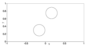
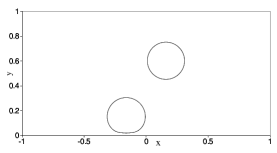
(a) (b) (c)

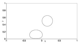
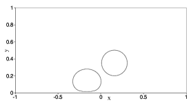
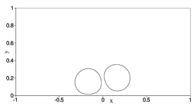
(d) (e) (f)

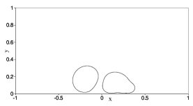
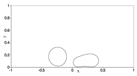
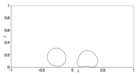
(g) (h) (i)

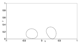
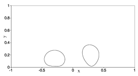
(j) (k) (l)

(m) (n) (o)

Figure 18: Impact of water/oil drops on horizontal wall with contact angles ($\theta_{ao},\theta_{aw})=(120^{0},150^{0})$: temporal sequence of snapshots of drop profiles at time instants (a) $t=0.0125$, (b) $t=0.1125$, (c) $t=0.175$, (d) $t=0.225$, (e) $t=0.2875$, (f) $t=0.3375$, (g) $t=0.375$, (h) $t=0.4375$, (i) $t=0.4625$, (j) $t=0.5$, (k) $t=0.525$, (l) $t=0.5625$, (m) $t=0.625$, (n) $t=0.6875$, (o) $t=0.75$.

In the second set of tests, the air-water contact angle is $\theta_{aw}=150^{0}$ (superhydrophobic wall surface), and the air-oil contact angle is the same as in the first set. Figure 18 shows a temporal sequence of snapshots of the fluid interfaces with this set of tests. The data depict a scenario similar to that of Figure 16, but with some main difference. After the impact, the water drop is observed to bounce off the wall and lift into the air while moving sideways in this case; see Figures 18(j)-(n). In contrast, in the first test case with $\theta_{aw}=120^{0}$ the water drop is observed to stay in contact with the wall and never bounce off after the impact; see Figures 16(j)-(n). Because the surface is more hydrophobic in the this case, small water drops can bounce off the wall upon impact, which is consistent with the observations in the two-phase bouncing water drop studies (see e.g. Dong2012 ; RichardQ2000 ).

(a) (b) (c)

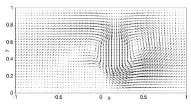
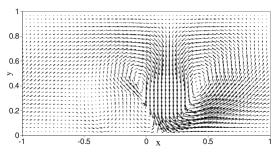
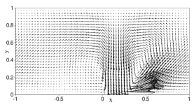
(d) (e) (f)

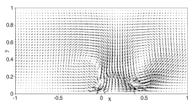
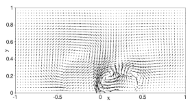
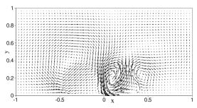
(g) (h) (i)

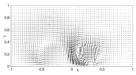
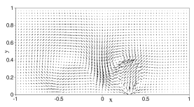
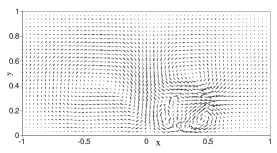
(j) (k) (l)

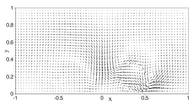
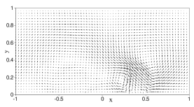
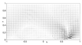
(m) (n) (o)

Figure 19: Water/oil drops impacting wall with contact angles ($\theta_{ao},\theta_{aw})=(120^{0},150^{0})$: temporal sequence of snapshots of the velocity fields at time instants (a) $t=0.0125$, (b) $t=0.1125$, (c) $t=0.175$, (d) $t=0.225$, (e) $t=0.2875$, (f) $t=0.3375$, (g) $t=0.375$, (h) $t=0.4375$, (i) $t=0.4625$, (j) $t=0.5$, (k) $t=0.525$, (l) $t=0.5625$, (m) $t=0.625$, (n) $t=0.6875$, (o) $t=0.75$. Velocity vectors are plotted on every ninth quadrature points in each direction within each element.

6 Concluding Remarks

In this paper we have explored the formulation and simulation of wall-bounded multiphase flows consisting of $N$ ($N\geqslant 2$) immiscible incompressible fluids with different densities, viscosities and pairwise surface tensions. We have looked into the implications of several reduction consistency properties between the $N$-phase formulation and the $M$-phase ($2\leqslant M\leqslant N-1$) formulations. We observe that the reduction consistency has profound implications on the N-phase governing equations, boundary conditions, and the form of the potential energy density function.

Our contributions can be specifically summarized in terms of the following aspects. First, we have presented a modified thermodynamically consistent phase field model for an N-fluid mixture that is more general than that of previous work Dong2014 . Second, by imposing the consistency property on the N-phase formulation we have obtained an explicit form for the mobility matrix in the phase field model. Third, by requiring the N-phase governing equations to be reduction consistent we have arrived at a set of conditions for the potential energy density function to ensure consistency. Fourth, we have proposed an N-phase contact-angle boundary condition that is reduction consistent with $M$-phase ($2\leqslant M\leqslant N-1$) systems.

The potential energy density function adopted in the current paper (originally suggested by BoyerM2014 ) ensures only a subset, yet an important subset, of the consistency conditions obtained herein. With this potential energy function, the N-phase formulation presented herein is fully consistent with two-phase formulations. In other words, if only a pair (for any pair) of fluid phases are present in the system, the N-phase physical formulation presented here will exactly reduce to the corresponding two-phase formulation. Compared with the previous N-phase formulations Dong2014 ; Dong2015 ), this is a great improvement, noting that both the current and the previous formulations are thermodynamically consistent.

Additionally, we have presented a numerical algorithm for solving the N-phase governing equations obtained herein. Employing this algorithm, we have performed extensive numerical experiments with several flow problems involving multiple flow components and partially wettable walls. Our simulation results show that the wall wettability and the contact angles have a profound influence on the equilibrium configuration and the dynamics of the multiphase system. In particular, we have compared our simulation results with the de Gennes theory deGennesBQ2003 about the contact angle effects on the spreading of a water drop and an oil drop on partially wettable wall surfaces. The comparison demonstrates that our method produces physically accurate results.

The method developed herein provides an effective technique for studying the interactions among multiple types of fluid interfaces and solid-wall surfaces, wettability effects, surface tension effects, and the dynamics and interactions of multiple types of contact lines. We anticipate that it will be useful to microfluidics, functional surfaces, materials processing, and applications in energy and petroleum industries.

The set of conditions on the potential energy density function (see (78a)–(78c)) ensures the consistency of the governing equations between the $N$-phase system and the $M$-phase systems ($2\leqslant M\leqslant N-1$). How does one construct a potential energy density function that satisfies all these conditions to ensure the full consistency? Is there some other way to ensure the reduction consistency between $N$ phases and $M$ phases ($2\leqslant M\leqslant N-1$)? These are interesting open questions to contemplate for future research.

Appendix A. Proof of Theorem 2.1

In light of assumption ($\mathcal{A}$1) about $H(\vec{\phi})$, it suffices to show that the term $\sum_{i,j=1}^{N-1}\frac{\lambda_{ij}}{2}\nabla\phi_{i}\cdot\nabla\phi_{j}$ in (26) satisfies the consistency property ($\mathcal{C}$2). Equation (28) implies $\sum_{i,j=1}^{N-1}\frac{\lambda_{ij}}{2}\nabla\phi_{i}\cdot\nabla\phi_{j}=\sum_{i,j=1}^{N-1}\frac{\Lambda_{ij}}{2}\nabla c_{i}\cdot\nabla c_{j}$ (see Dong2015 ), where $\phi_{i}$ ($1\leqslant i\leqslant N-1$) are a general set of order parameters defined by (22). So we only need to show that the term

$$K^{(N)}(\vec{c}^{(N)})=\sum_{i,j=1}^{N-1}\frac{\Lambda_{ij}^{(N)}}{2}\nabla c_{i}^{(N)}\cdot\nabla c_{j}^{(N)},\ \text{with}\ \Lambda_{ij}^{(N)}=\frac{3}{\sqrt{2}}\eta\left(\sigma_{iN}^{(N)}+\sigma_{jN}^{(N)}-\sigma_{ij}^{(N)}\right),\ 1\leqslant i,j\leqslant N-1,$$ (136)

satisfies ($\mathcal{C}$2), where $\vec{c}^{(N)}=(c_{1}^{(N)},c_{2}^{(N)},\dots,c_{N-1}^{(N)}),$ and the superscript in $(\cdot)^{(N)}$ accentuates the point that the quantity is for the $N$-phase system.

It suffices to show that, if one fluid phase is absent from the N-phase system then $K^{(N)}$ reduces to the corresponding form for the ($N-1$)-phase system. Let fluid $k$ ($1\leqslant k\leqslant N$) be the phase that is absent from the N-phase system, i.e. $c_{k}^{(N)}\equiv 0.$ We distinguish two cases: (i) $1\leqslant k\leqslant N-1$, and (ii) $k=N$.

In the first case ($1\leqslant k\leqslant N-1$), the first ($k-1$) fluids of the N-phase system have the same IDs in the ($N-1$)-phase system, and the last ($N-k$) fluids of the N-phase system will have their IDs reduced by one in the ($N-1$)-phase system. Therefore, the following relations hold

$$c_{i}^{(N-1)}=\left\{\begin{array}[]{ll}c_{i}^{(N)},&1\leqslant i\leqslant k-1,\\ c_{i+1}^{(N)},&k\leqslant i\leqslant N-1,\end{array}\right.$$ (137)

$$\sigma_{ij}^{(N-1)}=\left\{\begin{array}[]{ll}\sigma_{ij}^{(N)},&1\leqslant i\leqslant k-1,\ 1\leqslant j\leqslant k-1,\\ \sigma_{i,j+1}^{(N)},&1\leqslant i\leqslant k-1,\ k\leqslant j\leqslant N-1,\\ \sigma_{i+1,j}^{(N)},&k\leqslant i\leqslant N-1,\ 1\leqslant j\leqslant k-1,\\ \sigma_{i+1,j+1}^{(N)},&k\leqslant i\leqslant N-1,\ k\leqslant j\leqslant N-1,\end{array}\right.$$ (138)

$$\Lambda_{ij}^{(N-1)}=\frac{3}{\sqrt{2}}\eta\left(\sigma_{i,N-1}^{(N-1)}+\sigma_{j,N-1}^{(N-1)}-\sigma_{i,j}^{(N-1)}\right)\\ =\left\{\begin{array}[]{ll}\frac{3}{\sqrt{2}}\eta\left(\sigma_{iN}^{(N)}+\sigma_{jN}^{(N)}-\sigma_{ij}^{(N)}\right)=\Lambda_{ij}^{(N)},&1\leqslant i\leqslant k-1,\ 1\leqslant j\leqslant k-1,\\ \frac{3}{\sqrt{2}}\eta\left(\sigma_{iN}^{(N)}+\sigma_{j+1,N}^{(N)}-\sigma_{i,j+1}^{(N)}\right)=\Lambda_{i,j+1}^{(N)},&1\leqslant i\leqslant k-1,\ k\leqslant j\leqslant N-2,\\ \frac{3}{\sqrt{2}}\eta\left(\sigma_{i+1,N}^{(N)}+\sigma_{jN}^{(N)}-\sigma_{i+1,j}^{(N)}\right)=\Lambda_{i+1,j}^{(N)},&k\leqslant i\leqslant N-2,\ 1\leqslant j\leqslant k-1,\\ \frac{3}{\sqrt{2}}\eta\left(\sigma_{i+1,N}^{(N)}+\sigma_{j+1,N}^{(N)}-\sigma_{i+1,j+1}^{(N)}\right)=\Lambda_{i+1,j+1}^{(N)},&k\leqslant i\leqslant N-2,\ k\leqslant j\leqslant N-2.\end{array}\right.$$ (139)

Therefore,

$$\begin{split}&K^{(N)}(\vec{c}^{(N)})=\sum_{i,j=1}^{N-1}\frac{\Lambda_{ij}^{(N)}}{2}\nabla c_{i}^{(N)}\cdot\nabla c_{j}^{(N)}\\ =&\sum_{i,j=1}^{k-1}\frac{\Lambda_{ij}^{(N)}}{2}\nabla c_{i}^{(N)}\cdot\nabla c_{j}^{(N)}+\sum_{i=k+1}^{N-1}\sum_{j=1}^{k-1}\frac{\Lambda_{ij}^{(N)}}{2}\nabla c_{i}^{(N)}\cdot\nabla c_{j}^{(N)}\\ &\quad+\sum_{i=1}^{k-1}\sum_{j=k+1}^{N-1}\frac{\Lambda_{ij}^{(N)}}{2}\nabla c_{i}^{(N)}\cdot\nabla c_{j}^{(N)}+\sum_{i=k+1}^{N-1}\sum_{j=k+1}^{N-1}\frac{\Lambda_{ij}^{(N)}}{2}\nabla c_{i}^{(N)}\cdot\nabla c_{j}^{(N)}\\ =&\sum_{i,j=1}^{k-1}\frac{\Lambda_{ij}^{(N)}}{2}\nabla c_{i}^{(N)}\cdot\nabla c_{j}^{(N)}+\sum_{i=k}^{N-2}\sum_{j=1}^{k-1}\frac{\Lambda_{i+1,j}^{(N)}}{2}\nabla c_{i+1}^{(N)}\cdot\nabla c_{j}^{(N)}\\ &\quad+\sum_{i=1}^{k-1}\sum_{j=k}^{N-2}\frac{\Lambda_{i,j+1}^{(N)}}{2}\nabla c_{i}^{(N)}\cdot\nabla c_{j+1}^{(N)}+\sum_{i=k}^{N-2}\sum_{j=k}^{N-2}\frac{\Lambda_{i+1,j+1}^{(N)}}{2}\nabla c_{i+1}^{(N)}\cdot\nabla c_{j+1}^{(N)}\\ =&\sum_{i,j=1}^{k-1}\frac{\Lambda_{ij}^{(N-1)}}{2}\nabla c_{i}^{(N-1)}\cdot\nabla c_{j}^{(N-1)}+\sum_{i=k}^{N-2}\sum_{j=1}^{k-1}\frac{\Lambda_{ij}^{(N-1)}}{2}\nabla c_{i}^{(N-1)}\cdot\nabla c_{j}^{(N-1)}\\ &\quad+\sum_{i=1}^{k-1}\sum_{j=k}^{N-2}\frac{\Lambda_{ij}^{(N-1)}}{2}\nabla c_{i}^{(N-1)}\cdot\nabla c_{j}^{(N-1)}+\sum_{i=k}^{N-2}\sum_{j=k}^{N-2}\frac{\Lambda_{ij}^{(N-1)}}{2}\nabla c_{i}^{(N-1)}\cdot\nabla c_{j}^{(N-1)}\\ =&\sum_{i,j=1}^{N-2}\frac{\Lambda_{ij}^{(N-1)}}{2}\nabla c_{i}^{(N-1)}\cdot\nabla c_{j}^{(N-1)}\\ =&K^{(N-1)}(\vec{c}^{(N-1)}).\end{split}$$ (140)

In the second case ($k=N$), the first ($N-1$) fluids of the N-phase system have the same IDs in the ($N-1$)-phase system. Therefore, the following relations hold

$$c_{i}^{(N-1)}=c_{i}^{(N)},\quad 1\leqslant i\leqslant N-1,$$ (141)

$$\sum_{i=1}^{N-2}c_{i}^{(N)}+c_{N-1}^{(N)}=1,\quad\nabla c_{N-1}^{(N)}=-\sum_{i=1}^{N-2}\nabla c_{i}^{(N)},$$ (142)

$$\sigma_{ij}^{(N-1)}=\sigma_{ij}^{(N)},\quad 1\leqslant i,j\leqslant N-1,$$ (143)

$$\begin{split}\Lambda_{ij}^{(N)}&-\Lambda_{N-1,j}^{(N)}-\Lambda_{i,N-1}^{(N)}+\Lambda_{N-1,N-1}^{(N)}=\frac{3}{\sqrt{2}}\eta\left(\sigma_{i,N-1}^{(N)}+\sigma_{j,N-1}^{(N)}-\sigma_{ij}^{(N)}\right)\\ &=\frac{3}{\sqrt{2}}\eta\left(\sigma_{i,N-1}^{(N-1)}+\sigma_{j,N-1}^{(N-1)}-\sigma_{ij}^{(N-1)}\right)=\Lambda_{ij}^{(N-1)},\quad 1\leqslant i,j\leqslant N-2.\end{split}$$ (144)

Therefore,

$$\begin{split}&K^{(N)}(\vec{c}^{(N)})=\sum_{i,j=1}^{N-1}\frac{\Lambda_{ij}^{(N)}}{2}\nabla c_{i}^{(N)}\cdot\nabla c_{j}^{(N)}\\ =&\sum_{i,j=1}^{N-2}\frac{\Lambda_{ij}^{(N)}}{2}\nabla c_{i}^{(N)}\cdot\nabla c_{j}^{(N)}+\sum_{j=1}^{N-2}\frac{\Lambda_{N-1,j}^{(N)}}{2}\nabla c_{N-1}^{(N)}\cdot\nabla c_{j}^{(N)}\\ &\quad+\sum_{i=1}^{N-2}\frac{\Lambda_{i,N-1}^{(N)}}{2}\nabla c_{i}^{(N)}\cdot\nabla c_{N-1}^{(N)}+\frac{\Lambda_{N-1,N-1}^{(N)}}{2}\nabla c_{N-1}^{(N)}\cdot\nabla c_{N-1}^{(N)}\\ =&\sum_{i,j=1}^{N-2}\frac{1}{2}\left[\Lambda_{ij}^{(N)}-\Lambda_{N-1,j}^{(N)}-\Lambda_{i,N-1}^{(N)}+\Lambda_{N-1,N-1}^{(N)}\right]\nabla c_{i}^{(N)}\cdot\nabla c_{j}^{(N)}\\ =&\sum_{i,j=1}^{N-2}\frac{1}{2}\Lambda_{ij}^{(N-1)}\nabla c_{i}^{(N-1)}\cdot\nabla c_{j}^{(N-1)}\\ =&K^{(N-1)}(\vec{c}^{(N-1)}).\end{split}$$ (145)

Appendix B. Proof of Theorem 2.2

Suppose fluid $k$ (for any $1\leqslant k\leqslant N$) is absent from the N-phase system. Then we have the following relations

$$\tilde{\rho}_{i}^{(N-1)}=\left\{\begin{array}[]{ll}\tilde{\rho}_{i}^{(N)},&1\leqslant i\leqslant k-1\\ \tilde{\rho}_{i+1}^{(N)},&k\leqslant i\leqslant N-1,\end{array}\right.\tilde{\mu}_{i}^{(N-1)}=\left\{\begin{array}[]{ll}\tilde{\mu}_{i}^{(N)},&1\leqslant i\leqslant k-1\\ \tilde{\mu}_{i+1}^{(N)},&k\leqslant i\leqslant N-1.\end{array}\right.$$ (146)

According to (6),

$$\begin{split}\rho^{(N)}&=\sum_{i=1}^{N}\tilde{\rho}_{i}^{(N)}c_{i}^{(N)}=\sum_{i=1}^{k-1}\tilde{\rho}_{i}^{(N)}c_{i}^{(N)}+\sum_{i=k+1}^{N}\tilde{\rho}_{i}^{(N)}c_{i}^{(N)}=\sum_{i=1}^{k-1}\tilde{\rho}_{i}^{(N-1)}c_{i}^{(N-1)}+\sum_{i=k+1}^{N}\tilde{\rho}_{i-1}^{(N-1)}c_{i-1}^{(N-1)}\\ &=\sum_{i=1}^{k-1}\tilde{\rho}_{i}^{(N-1)}c_{i}^{(N-1)}+\sum_{i=k}^{N-1}\tilde{\rho}_{i}^{(N-1)}c_{i}^{(N-1)}=\sum_{i=1}^{N-1}\tilde{\rho}_{i}^{(N-1)}c_{i}^{(N-1)}=\rho^{(N-1)}.\end{split}$$ (147)

So equation (79) holds.

It can be similarly shown that equation (80) holds in light of equation (19),

$$\begin{split}\mu^{(N)}&=\sum_{i=1}^{N}\tilde{\mu}_{i}^{(N)}c_{i}^{(N)}=\sum_{i=1}^{k-1}\tilde{\mu}_{i}^{(N)}c_{i}^{(N)}+\sum_{i=k+1}^{N}\tilde{\mu}_{i}^{(N)}c_{i}^{(N)}=\sum_{i=1}^{k-1}\tilde{\mu}_{i}^{(N-1)}c_{i}^{(N-1)}+\sum_{i=k+1}^{N}\tilde{\mu}_{i-1}^{(N-1)}c_{i-1}^{(N-1)}\\ &=\sum_{i=1}^{k-1}\tilde{\mu}_{i}^{(N-1)}c_{i}^{(N-1)}+\sum_{i=k}^{N-1}\tilde{\mu}_{i}^{(N-1)}c_{i}^{(N-1)}=\sum_{i=1}^{N-1}\tilde{\mu}_{i}^{(N-1)}c_{i}^{(N-1)}=\mu^{(N-1)}.\end{split}$$ (148)

In Appendix A we have shown that the term $K^{(N)}=\sum_{i,j=1}^{N-1}\frac{1}{2}\Lambda_{ij}^{(N)}\nabla c_{i}^{(N)}\cdot\nabla c_{j}^{(N)}$ (see (136)) reduces to the corresponding form $K^{(N-1)}$ of the ($N-1$)-phase system if one fluid phase is absent. Using a procedure parallel to that for $K^{(N)}$, one can show that $\sum_{i,j=1}^{N-1}\Lambda_{ij}^{(N)}\nabla c_{i}^{(N)}\otimes\nabla c_{j}^{(N)}=\sum_{i,j=1}^{N-2}\Lambda_{ij}^{(N-1)}\nabla c_{i}^{(N-1)}\otimes\nabla c_{j}^{(N-1)}.$ Therefore relation (81) holds.

We next show that the relation (82) holds provided that the conditions (78a)–(78c) are satisfied by $H(\vec{\phi})$. We use the volume fractions as the order parameters as defined by (24). Based on equations (71) and (75) and noting $\sum_{i=1}^{N-1}\left(1-\frac{N}{\Gamma}\tilde{\gamma}_{i}\right)a_{ij}=\tilde{\rho}_{j}-\tilde{\rho}_{N},$ where $a_{ij}$ are given by (25), we have

$$\begin{split}\tilde{\mathbf{J}}^{(N)}&=-m_{0}\sum_{j=1}^{N-1}\left[\sum_{i=1}^{N-1}\left(1-\frac{N}{\Gamma^{(N)}}\tilde{\gamma}_{i}^{(N)}\right)a_{ij}^{(N)}\right]\nabla\left(-\nabla^{2}c_{j}^{(N)}+L_{j}^{(N)}\right)\\ &=-m_{0}\sum_{j=1}^{N-1}\left(\tilde{\rho}_{j}^{(N)}-\tilde{\rho}_{N}^{(N)}\right)\nabla\left(-\nabla^{2}c_{j}^{(N)}+L_{j}^{(N)}\right).\end{split}$$ (149)

Let $c_{k}^{(N)}\equiv 0$ for some $k$ ($1\leqslant k\leqslant N$), and assume that the conditions (78a)–(78c) are satisfied by $H(\vec{\phi})$. We distinguish two cases: (i) $1\leqslant k\leqslant N-1$, and (ii) $k=N$.

In the first case, we have the correspondence relations given by (146), (137) and (78b)–(78c). Therefore,

$$\begin{split}\tilde{\mathbf{J}}^{(N)}&=-m_{0}\left(\sum_{j=1}^{k-1}+\sum_{j=k+1}^{N-1}\right)\left(\tilde{\rho}_{j}^{(N)}-\tilde{\rho}_{N}^{(N)}\right)\nabla\left(-\nabla^{2}c_{j}^{(N)}+L_{j}^{(N)}\right)\\ &=-m_{0}\sum_{j=1}^{k-1}\left(\tilde{\rho}_{j}^{(N)}-\tilde{\rho}_{N}^{(N)}\right)\nabla\left(-\nabla^{2}c_{j}^{(N)}+L_{j}^{(N)}\right)-m_{0}\sum_{j=k}^{N-2}\left(\tilde{\rho}_{j+1}^{(N)}-\tilde{\rho}_{N}^{(N)}\right)\nabla\left(-\nabla^{2}c_{j+1}^{(N)}+L_{j+1}^{(N)}\right)\\ &=-m_{0}\left(\sum_{j=1}^{k-1}+\sum_{j=k}^{N-2}\right)\left(\tilde{\rho}_{j}^{(N-1)}-\tilde{\rho}_{N-1}^{(N-1)}\right)\nabla\left(-\nabla^{2}c_{j}^{(N-1)}+L_{j}^{(N-1)}\right)\\ &=\tilde{\mathbf{J}}^{(N-1)},\end{split}$$ (150)

where we have used (78a).

In the second case ($k=N$) we have the relations given by (141)–(142) and

$$\tilde{\rho}_{i}^{(N-1)}=\tilde{\rho}_{i}^{(N)},\quad 1\leqslant i\leqslant N-1.$$ (151)

Combining (78a) and (75) leads to

$$0=\nabla L_{N}^{(N)}=-\sum_{i=1}^{N-2}\nabla L_{i}^{(N)}-\nabla L_{N-1}^{(N)},\quad\nabla L_{N-1}^{(N)}=-\sum_{i=1}^{N-2}\nabla L_{i}^{(N)}.$$ (152)

Therefore,

$$\begin{split}\tilde{\mathbf{J}}^{(N)}&=-m_{0}\sum_{j=1}^{N-2}\left(\tilde{\rho}_{j}^{(N)}-\tilde{\rho}_{N}^{(N)}\right)\nabla\left(-\nabla^{2}c_{j}^{(N)}+L_{j}^{(N)}\right)-m_{0}\left(\tilde{\rho}_{N-1}^{(N)}-\tilde{\rho}_{N}^{(N)}\right)\nabla\left(-\nabla^{2}c_{N-1}^{(N)}+L_{N-1}^{(N)}\right)\\ &=-m_{0}\sum_{j=1}^{N-2}\left(\tilde{\rho}_{j}^{(N)}-\tilde{\rho}_{N}^{(N)}\right)\nabla\left(-\nabla^{2}c_{j}^{(N)}+L_{j}^{(N)}\right)+m_{0}\sum_{j=1}^{N-2}\left(\tilde{\rho}_{N-1}^{(N)}-\tilde{\rho}_{N}^{(N)}\right)\nabla\left(-\nabla^{2}c_{j}^{(N)}+L_{j}^{(N)}\right)\\ &=-m_{0}\sum_{j=1}^{N-2}\left(\tilde{\rho}_{j}^{(N)}-\tilde{\rho}_{N-1}^{(N)}\right)\nabla\left(-\nabla^{2}c_{j}^{(N)}+L_{j}^{(N)}\right)\\ &=-m_{0}\sum_{j=1}^{N-2}\left(\tilde{\rho}_{j}^{(N-1)}-\tilde{\rho}_{N-1}^{(N-1)}\right)\nabla\left(-\nabla^{2}c_{j}^{(N-1)}+L_{j}^{(N-1)}\right)\\ &=\tilde{\mathbf{J}}^{(N-1)},\end{split}$$ (153)

where we have used (78a)–(78b), (141)–(142), and (152).

Appendix C. Proof of Theorem 2.3

Suppose fluid $k$ and fluid $l$ ($1\leqslant k<l\leqslant N$) are the only fluid phases present in the N-phase system. Then the system is characterized by the conditions listed in (34).

For the two-phase system consisting of fluids $k$ and $l$, we have thses relations,

$$\left\{\begin{split}&c_{1}^{(2)}=c_{k},\quad c_{2}^{(2)}=c_{l},\quad\tilde{\rho}_{1}^{(2)}=\tilde{\rho}_{k},\quad\tilde{\rho}_{2}^{(2)}=\tilde{\rho}_{l},\quad\sigma_{12}^{(2)}=\sigma_{kl},\quad\\ &\Lambda_{11}^{(2)}=\frac{6}{\sqrt{2}}\eta\sigma_{12}^{(2)},\quad\Theta_{11}^{(2)}=\frac{1}{\Lambda_{11}^{(2)}}=\frac{\sqrt{2}}{6\eta}\frac{1}{\sigma_{12}^{(2)}},\\ &H^{(2)}=\beta\sigma_{12}^{(2)}f(c_{1}^{(2)}),\end{split}\right.$$ (154)

where $\beta$ is given by (37), the superscript in $(\cdot)^{(2)}$ refers to the variable for the corresponding two-phase system, and we have used (83), (42) and (73). As a result,

$$\left\{\begin{split}&L_{1}^{(2)}=\Theta_{11}^{(2)}\frac{\partial H^{(2)}}{\partial c_{1}^{(2)}}=\frac{\sqrt{2}}{6\eta}\beta f^{\prime}(c_{1}^{(2)})=\frac{1}{\eta^{2}}f^{\prime}(c_{k})\\ &L_{2}^{(2)}=-L_{1}^{(2)}=-\frac{1}{\eta^{2}}f^{\prime}(c_{k}),\end{split}\right.$$ (155)

where we have used (75).

For the N-phase system characterized by (34), we first note several simple facts that would be useful for the following discussions (where $f(c)$ is given in (83)):

$$f(c)=f(1-c),\quad f^{\prime}(c)=-f^{\prime}(1-c),\quad f(0)=f(1)=0,\quad f^{\prime}(0)=f^{\prime}(1)=0;$$ (156a)

$$c_{k}+c_{l}=1,\quad f(c_{k})=f(c_{l}),\quad f^{\prime}(c_{k})=-f^{\prime}(c_{l}),\quad f(c_{k}+c_{l})=f^{\prime}(c_{k}+c_{l})=0;$$ (156b)

$$f(c_{i})=f^{\prime}(c_{i})=0,\ \text{if}\ i\neq k\ \text{and}\ i\neq l,\ \text{for}\ 1\leqslant i\leqslant N.$$ (156c)

In light of (83) we get

$$\frac{2}{\beta}\frac{\partial H}{\partial c_{i}}=\sigma_{i}f^{\prime}(c_{i})-\sigma_{N}f^{\prime}(c_{N})-\sum_{j=1}^{N}\sigma_{ij}f^{\prime}(c_{i}+c_{j})+\sum_{j=1}^{N}\sigma_{Nj}f^{\prime}(c_{N}+c_{j}),\quad 1\leqslant i\leqslant N-1,$$ (157)

where

$$\sigma_{i}=\sum_{j=1}^{N}\sigma_{ij},\quad 1\leqslant i\leqslant N.$$ (158)

Note that when computing $\frac{\partial H}{\partial c_{i}}$ ($1\leqslant i\leqslant N-1$) one must treat $c_{N}$ as a variable dependent on $c_{i}$ ($1\leqslant i\leqslant N-1$), i.e. $c_{N}=1-\sum_{i=1}^{N-1}c_{i}.$ Note also that we have not included the superscript $(N)$ for brevity in the above expressions, and in subsequent discussions we will also drop this superscript if no confusion arises. Therefore,

$$\begin{split}\frac{2}{\beta}L_{i}^{(N)}&=\frac{2}{\beta}\sum_{j=1}^{N-1}\Theta_{ij}\frac{\partial H}{\partial c_{j}}\\ &=\sum_{j=1}^{N-1}\Theta_{ij}\sigma_{j}f^{\prime}(c_{j})-\Theta_{i}\sigma_{N}f^{\prime}(c_{N})-\sum_{j=1}^{N-1}\sum_{s=1}^{N}\Theta_{ij}\sigma_{js}f^{\prime}(c_{j}+c_{s})+\Theta_{i}\sum_{j=1}^{N}\sigma_{Nj}f^{\prime}(c_{N}+c_{j}),\\ &\quad 1\leqslant i\leqslant N-1,\end{split}$$ (159)

where

$$\Theta_{i}=\sum_{j=1}^{N-1}\Theta_{ij},\quad 1\leqslant i\leqslant N-1.$$ (160)

We distinguish two cases: (i) $1\leqslant k<l\leqslant N-1$, and (ii) $1\leqslant k<l=N$. In the first case,

$$\sum_{j=1}^{N-1}\sum_{s=1}^{N}\Theta_{ij}\sigma_{js}f^{\prime}(c_{j}+c_{s})=\Theta_{ik}\sigma_{k}f^{\prime}(c_{k})+\Theta_{il}\sigma_{l}f^{\prime}(c_{l})+\sum_{j=1}^{N-1}\Theta_{ij}\sigma_{jk}f^{\prime}(c_{k})+\sum_{j=1}^{N-1}\Theta_{ij}\sigma_{jl}f^{\prime}(c_{l}),$$ (161)

where we have used (34), and (156b)–(156c). Equation (159) is then transformed into

$$\frac{2}{\beta}L_{i}^{(N)}=\Theta_{i}\sigma_{Nk}f^{\prime}(c_{k})+\Theta_{i}\sigma_{Nl}f^{\prime}(c_{l})-\sum_{j=1}^{N-1}\Theta_{ij}\sigma_{jk}f^{\prime}(c_{k})-\sum_{j=1}^{N-1}\Theta_{ij}\sigma_{jl}f^{\prime}(c_{l}),\quad 1\leqslant i\leqslant N-1,$$ (162)

where we have used (156b) and (156c). In light of (73), we have the relations

$$\left\{\begin{split}&\delta_{ij}=\sum_{s=1}^{N-1}\Theta_{is}\Lambda_{sj}=\frac{3}{\sqrt{2}}\eta\sum_{s=1}^{N-1}\Theta_{is}\left(\sigma_{sN}+\sigma_{jN}-\sigma_{sj}\right),\\ &\sum_{s=1}^{N-1}\Theta_{is}\sigma_{sj}=\Theta_{i}\sigma_{jN}+\sum_{s=1}^{N-1}\Theta_{is}\sigma_{sN}-\frac{\sqrt{2}}{3\eta}\delta_{ij},\quad 1\leqslant i,j\leqslant N-1,\end{split}\right.$$ (163)

where we have used (42) and $\delta_{ij}$ is the Kronecker delta. Therefore, equation (162) is transformed into

$$\frac{2}{\beta}L_{i}^{(N)}=\frac{\sqrt{2}}{3\eta}\delta_{ik}f^{\prime}(c_{k})+\frac{\sqrt{2}}{3\eta}\delta_{il}f^{\prime}(c_{l})=\frac{\sqrt{2}}{3\eta}(\delta_{ik}-\delta_{il})f^{\prime}(c_{k}),\quad 1\leqslant i\leqslant N-1.$$ (164)

As a result,

$$\left\{\begin{split}&L_{i}^{(N)}=\frac{1}{\eta^{2}}(\delta_{ik}-\delta_{il})f^{\prime}(c_{k}),\quad\quad 1\leqslant i\leqslant N-1,\\ &L_{N}^{(N)}=-\sum_{i=1}^{N-1}L_{i}^{(N)}=-L_{k}^{(N)}-L_{l}^{(N)}=-\frac{1}{\eta^{2}}f^{\prime}(c_{k})+\frac{1}{\eta^{2}}f^{\prime}(c_{k})=0,\end{split}\right.$$ (165)

where we have used (37) and (75). Comparing equations (165) and (155), we conclude that the relations (84a)–(84c) hold for this case.

In the second case ($1\leqslant k<l=N$),

$$\sum_{j=1}^{N-1}\sum_{s=1}^{N}\Theta_{ij}\sigma_{js}f^{\prime}(c_{j}+c_{s})=\Theta_{ik}\sigma_{k}f^{\prime}(c_{k})+\sum_{j=1}^{N-1}\Theta_{ij}\sigma_{jk}f^{\prime}(c_{k})+\sum_{j=1}^{N-1}\Theta_{ij}\sigma_{jN}f^{\prime}(c_{N}),$$ (166)

where we have used (156b)–(156c), (34) and (35). Therefore, equation (159) is transformed into

$$\frac{2}{\beta}L_{i}^{(N)}=-\sum_{j=1}^{N-1}\Theta_{ij}\sigma_{jk}f^{\prime}(c_{k})-\sum_{j=1}^{N-1}\Theta_{ij}\sigma_{jN}f^{\prime}(c_{N})-\Theta_{i}\sigma_{Nk}f^{\prime}(c_{N}),\quad 1\leqslant i\leqslant N-1,$$ (167)

where we have used (156b) and (156c). In light of (163), we have

$$\sum_{j=1}^{N-1}\Theta_{ij}\sigma_{jk}=\Theta_{i}\sigma_{kN}+\sum_{j=1}^{N-1}\Theta_{ij}\sigma_{jN}-\frac{\sqrt{2}}{3\eta}\delta_{ik}.$$ (168)

Substitute this expression into (167), and we get

$$\left\{\begin{split}&L_{i}^{(N)}=\frac{\beta}{2}\frac{\sqrt{2}}{3\eta}\delta_{ik}f^{\prime}(c_{k})=\frac{1}{\eta^{2}}\delta_{ik}f^{\prime}(c_{k}),\quad 1\leqslant i\leqslant N-1,\\ &L_{N}^{(N)}=-\sum_{i=1}^{N-1}L_{i}^{(N)}=-L_{k}^{(N)}=-\frac{1}{\eta^{2}}f^{\prime}(c_{k}),\end{split}\right.$$ (169)

where we have used (156b), (37) and (75). Comparing the equations (169) and (155), we conclude that the relations (84a)–(84c) hold for the second case.

From the above discussions we note the following relation

$$L_{k}^{(N)}+L_{l}^{(N)}=0$$ (170)

for the N-phase system characterized by (34).

Finaly let us consider the relation (84d). We again distinguish two cases: (i) $1\leqslant k<l\leqslant N-1$, (ii) $1\leqslant k<l=N$. In the first case, according to (149),

$$\begin{split}\tilde{\mathbf{J}}^{(N)}&=-m_{0}\sum_{j=1}^{N-1}\left(\tilde{\rho}_{j}-\tilde{\rho}_{N}\right)\nabla\left(-\nabla^{2}c_{j}+L_{j}^{(N)}\right)\\ &=-m_{0}\left(\tilde{\rho}_{k}-\tilde{\rho}_{N}\right)\nabla\left(-\nabla^{2}c_{k}+L_{k}^{(N)}\right)-m_{0}\left(\tilde{\rho}_{l}-\tilde{\rho}_{N}\right)\nabla\left(-\nabla^{2}c_{l}+L_{l}^{(N)}\right)\\ &=-m_{0}\tilde{\rho}_{k}\nabla\left(-\nabla^{2}c_{k}+L_{k}^{(N)}\right)-m_{0}\tilde{\rho}_{l}\nabla\left(-\nabla^{2}c_{l}+L_{l}^{(N)}\right)\\ &=-m_{0}\left(\tilde{\rho}_{k}-\tilde{\rho}_{l}\right)\nabla\left(-\nabla^{2}c_{k}+L_{k}^{(N)}\right)\\ &=-m_{0}\left(\tilde{\rho}_{1}^{(2)}-\tilde{\rho}_{2}^{(2)}\right)\nabla\left(-\nabla^{2}c_{1}^{(2)}+L_{1}^{(2)}\right)\\ &=\tilde{\mathbf{J}}^{(2)},\end{split}$$ (171)

where we have used (84a)–(84c) and (170). In the second case,

$$\begin{split}\tilde{\mathbf{J}}^{(N)}&=-m_{0}\sum_{j=1}^{N-1}\left(\tilde{\rho}_{j}-\tilde{\rho}_{N}\right)\nabla\left(-\nabla^{2}c_{j}+L_{j}^{(N)}\right)\\ &=-m_{0}\left(\tilde{\rho}_{k}-\tilde{\rho}_{N}\right)\nabla\left(-\nabla^{2}c_{k}+L_{k}^{(N)}\right)\\ &=-m_{0}\left(\tilde{\rho}_{k}-\tilde{\rho}_{l}\right)\nabla\left(-\nabla^{2}c_{k}+L_{k}^{(N)}\right)\\ &=-m_{0}\left(\tilde{\rho}_{1}^{(2)}-\tilde{\rho}_{2}^{(2)}\right)\nabla\left(-\nabla^{2}c_{1}^{(2)}+L_{1}^{(2)}\right)\\ &=\tilde{\mathbf{J}}^{(2)},\end{split}$$ (172)

where we have used (84a)–(84c).

Appendix D. Algorithm for N-Phase Momentum Equations

In this Appendix we provide a summary of the algorithm we developed in Dong2015 for the N-phase momentum equations, (109) and (4), together with the velocity boundary condition, (108). We assume that the phase field variables $\phi_{i}^{n+1}$ ($1\leqslant i\leqslant N-1$) are already computed using the algorithm from Section 4, and our goal here is to compute the velocity and pressure from (109) and (4).

Given ($\mathbf{u}^{n}$, $P^{n}$, $\phi_{i}^{n+1}$), we solve (109) and (4) by successively computing $P^{n+1}$ and $\mathbf{u}^{n+1}$ in a de-coupled fashion as follows:
For $P^{n+1}$:

$$\begin{split}\frac{\gamma_{0}\tilde{\mathbf{u}}^{n+1}-\hat{\mathbf{u}}}{\Delta t}+\mathbf{u}^{*,n+1}\cdot\nabla\mathbf{u}^{*,n+1}&+\frac{1}{\rho^{n+1}}\tilde{\mathbf{J}}^{n+1}\cdot\nabla\mathbf{u}^{*,n+1}+\frac{1}{\rho_{0}}\nabla P^{n+1}=\left(\frac{1}{\rho_{0}}-\frac{1}{\rho^{n+1}}\right)\nabla P^{*,n+1}\\ &-\frac{\mu^{n+1}}{\rho^{n+1}}\nabla\times\nabla\times\mathbf{u}^{*,n+1}+\frac{1}{\rho^{n+1}}\nabla\mu^{n+1}\cdot\mathbf{D}(\mathbf{u}^{*,n+1})\\ &-\frac{1}{\rho^{n+1}}\sum_{i,j=1}^{N-1}\lambda_{ij}\nabla^{2}\phi_{j}^{n+1}\nabla\phi_{i}^{n+1}+\frac{1}{\rho^{n+1}}\mathbf{f}^{n+1},\end{split}$$ (173a)

$$\nabla\cdot\tilde{\mathbf{u}}^{n+1}=0,$$ (173b)

$$\left.\mathbf{n}\cdot\tilde{\mathbf{u}}^{n+1}\right|_{\partial\Omega}=\mathbf{n}\cdot\mathbf{w}^{n+1}.$$ (173c)

For $\mathbf{u}^{n+1}$:

$$\frac{\gamma_{0}\mathbf{u}^{n+1}-\gamma_{0}\tilde{\mathbf{u}}^{n+1}}{\Delta t}-\nu_{0}\nabla^{2}\mathbf{u}^{n+1}=\nu_{0}\nabla\times\nabla\times\mathbf{u}^{*,n+1},$$ (174a)

$$\left.\mathbf{u}^{n+1}\right|_{\partial\Omega}=\mathbf{w}^{n+1}.$$ (174b)

In the above equations all the symbols follow the notation outlined in Section 4. $\mathbf{u}^{*,n+1}$ and $P^{*,n+1}$ are defined by (116). $\hat{\mathbf{u}}$ and $\gamma_{0}$ are defined by (117). $\rho^{n+1}$ and $\mu^{n+1}$ are given by (129), and also (130) in case of large density ratios among the N fluids. $\tilde{\mathbf{J}}^{n+1}$ is given by (71). $\mathbf{f}^{n+1}$ is the external body force evaluated at time step ($n+1$). $\mathbf{n}$ is the outward-pointing unit vector normal to $\partial\Omega$. $\tilde{\mathbf{u}}^{n+1}$ is an auxiliary velocity that approximates $\mathbf{u}^{n+1}$. $\rho_{0}$ is a chosen constant that must satisfy the condition

$$0<\rho_{0}\leqslant\min(\tilde{\rho}_{1},\tilde{\rho}_{2},\dots,\tilde{\rho}_{N}).$$ (175)

$\nu_{0}$ in (174a) is a chosen positive constant that is sufficiently large. In the current paper we employ an $\nu_{0}$ value with the following,

$$\nu_{0}\geqslant\max\left(\frac{\tilde{\mu}_{1}}{\tilde{\rho}_{1}},\frac{\tilde{\mu}_{2}}{\tilde{\rho}_{2}},\cdots,\frac{\tilde{\mu}_{N}}{\tilde{\rho}_{N}},\right).$$ (176)

The above algorithm employs a velocity correction-type idea DongS2010 ; DongKC2014 ; Dong2015clesobc to de-couple the computations for the pressure and the velocity. It can be noted that the variable density $\rho$ and the variable dynamic viscosity $\mu$ have been treated with a reformulation of the pressure term $\frac{1}{\rho}\nabla P$ and a reformulation of the viscous term $\frac{\mu}{\rho}\nabla^{2}\mathbf{u}$, so that the linear algebraic systems resulting from the discretization involve only constant and time-independent coefficient matrices. The ideas for the reformulations stem from the original developments for two-phase flows DongS2012 ; Dong2012 ; Dong2014obc .

Le us next derive the weak forms for the pressure and the velocity in order to facilitate the implementation using $C^{0}$ spectral elements. Let $q\in H^{1}(\Omega)$ denote the test function, and let

$$\mathbf{G}^{n+1}=\frac{1}{\rho^{n+1}}\mathbf{f}^{n+1}-\left(\mathbf{u}^{*,n+1}+\frac{1}{\rho^{n+1}}\tilde{\mathbf{J}}^{n+1}\right)\cdot\nabla\mathbf{u}^{*,n+1}+\frac{\hat{\mathbf{u}}}{\Delta t}+\left(\frac{1}{\rho_{0}}-\frac{1}{\rho^{n+1}}\right)\nabla P^{*,n+1}\\ +\frac{1}{\rho^{n+1}}\nabla\mu^{n+1}\cdot\mathbf{D}(\mathbf{u}^{*,n+1})-\frac{1}{\rho^{n+1}}\sum_{i,j=1}^{N-1}\lambda_{ij}\nabla^{2}\phi_{j}^{n+1}\nabla\phi_{i}^{n+1}+\nabla\left(\frac{\mu^{n+1}}{\rho^{n+1}}\right)\times\bm{\omega}^{*,n+1},$$ (177)

where $\bm{\omega}=\nabla\times\mathbf{u}$ is the vorticity. Take the $L^{2}$ inner product between equation (173a) and $\nabla q$, and we get the weak form about $P^{n+1}$,

$$\int_{\Omega}\nabla P^{n+1}\cdot\nabla q=\rho_{0}\int_{\Omega}\mathbf{G}^{n+1}\cdot\nabla q-\rho_{0}\int_{\partial\Omega}\frac{\mu^{n+1}}{\rho^{n+1}}\mathbf{n}\times\bm{\omega}^{*,n+1}\cdot\nabla q-\frac{\gamma_{0}\rho_{0}}{\Delta t}\int_{\partial\Omega}\mathbf{n}\cdot\mathbf{w}^{n+1}q,\ \ \forall q\in H^{1}(\Omega)$$ (178)

where we have used integration by part, equations (173b) and (173c), the divergence theorem, and the identity $\frac{\mu}{\rho}\nabla\times\bm{\omega}\cdot\nabla q=\nabla\cdot\left(\frac{\mu}{\rho}\bm{\omega}\times\nabla q\right)-\nabla\left(\frac{\mu}{\rho}\right)\times\bm{\omega}\cdot\nabla q.$

Adding together the equations (173a) and (174a), we get

$$\frac{\gamma_{0}}{\Delta t}\mathbf{u}^{n+1}-\nu_{0}\nabla^{2}\mathbf{u}^{n+1}=\mathbf{G}^{n+1}-\nabla\left(\frac{\mu^{n+1}}{\rho^{n+1}}\right)\times\bm{\omega}^{*,n+1}-\frac{1}{\rho_{0}}\nabla P^{n+1}-\left(\frac{\mu^{n+1}}{\rho^{n+1}}-\nu_{0}\right)\nabla\times\bm{\omega}^{*,n+1}$$ (179)

Let $H^{1}_{0}(\Omega)=\left\{\ v\in H^{\Omega}\ :\ v|_{\partial\Omega}=0\ \right\},$ and $\varphi\in H_{0}^{1}(\Omega)$ denote the test function. Taking the $L^{2}$ inner product between equation (179) and $\varphi$, one can get the weak form about $\mathbf{u}^{n+1}$,

$$\int_{\Omega}\nabla\varphi\cdot\nabla\mathbf{u}^{n+1}+\frac{\gamma_{0}}{\nu_{0}\Delta t}\int_{\Omega}\varphi\mathbf{u}^{n+1}=\frac{1}{\nu_{0}}\int_{\Omega}\left(\mathbf{G}^{n+1}-\frac{1}{\rho_{0}}\nabla P^{n+1}\right)\varphi\\ -\frac{1}{\nu_{0}}\int_{\Omega}\left(\frac{\mu^{n+1}}{\rho^{n+1}}-\nu_{0}\right)\bm{\omega}^{*,n+1}\times\nabla\varphi,\qquad\forall\varphi\in H_{0}^{1}(\Omega),$$ (180)

where we have used integration by part, the divergence theorem, the identity ($\chi$ denoting a scalar function)

$$\int_{\Omega}\chi\nabla\times\bm{\omega}\varphi=\int_{\partial\Omega}\chi\mathbf{n}\times\bm{\omega}\varphi-\int_{\Omega}\nabla\chi\times\bm{\omega}\varphi+\int_{\Omega}\chi\bm{\omega}\times\nabla\varphi,$$

and the fact that the surface integrals of type $\int_{\partial\Omega}\chi\varphi$ vanish because $\varphi\in H^{1}_{0}(\Omega)$.

The weak forms for the pressure and the velocity, (178) and (180), can be discretized in space using $C^{0}$ spectral elements in a straightforward fashion. Note that the terms $\nabla^{2}\phi_{i}^{n+1}$ ($1\leqslant i\leqslant N-1$) involved in the $\mathbf{G}^{n+1}$ expression (177) and in the $\tilde{\mathbf{J}}^{n+1}$ expression (see (149) and (71)) must be computed based on equation (127).

Solving the N-phase momentum equations (109) and (4) amounts to the following two successive operations. First, solve equation (178) for pressure $P^{n+1}$. Then, solve equation (180), together with the Dirichlet condition (174b) on $\partial\Omega$, for $\mathbf{u}^{n+1}$.

References

- [1] D.M. Anderson, G.B. McFadden, and A.A. Wheeler. Diffuse-interface methods in fluid mechanics. Annu. Rev. Fluid Mech., 30:139–165, 1998.
- [2] M.J. Blunt. Constraints on contact angles for multiple phases in thermodynamic equilibrium. Journal of Colloid and Interface Science, 239:281–282, 2001.
- [3] F. Boyer and C. Lapuerta. Study of a three component cahn-hilliard flow model. ESAIM: M2AN, 40:653–687, 2006.
- [4] F. Boyer, C. Lapuerta, S. Minjeaud, B. Piar, and M. Quintard. Cahn-hilliard/navier-stokes model for the simulation of three-phase flows. Transp. Porous Med., 82:463–483, 2010.
- [5] F. Boyer and S. Minjeaud. Numerical schemes for a three component cahn-hilliard model. ESAIM: M2AN, 45:697–738, 2011.
- [6] F. Boyer and S. Minjeaud. Hierarchy of consistent n-component Cahn-Hilliard systems. Mathematical Models and Methods in Applied Sciences, 24:2885–2928, 2014.
- [7] A. Carlson, M. Do-Quang, and G. Amberg. Dissipation in rapid dynamic wetting. J. Fluid Mech., 682, 2011.
- [8] P.G. de Gennes, F. Brochard-Wyart, and D. Quere. Capillarity and Wetting Phenomena. Springer, 2003.
- [9] S. Dong. On imposing dynamic contact-angle boundary conditions for wall-bounded liquid-gas flows. Computer Methods in Applied Mechanics and Engineering, 247–248:179–200, 2012.
- [10] S. Dong. An efficient algorithm for incompressible N-phase flows. Journal of Computational Physics, 276:691–728, 2014.
- [11] S. Dong. An outflow boundary condition and algorithm for incompressible two-phase flows with phase field approach. Journal of Computational Physics, 266:47–73, 2014.
- [12] S. Dong. A convective-like energy-stable open boundary condition for simulations of incompressible flows. Journal of Computational Physics, 302:300–328, 2015.
- [13] S. Dong. Physical formulation and numerical algorithm for simulating N immiscible incompressible fluids involving general order parameters. Journal of Computational Physics, 283:98–128, 2015.
- [14] S. Dong, G.E. Karniadakis, and C. Chryssostomidis. A robust and accurate outflow boundary condition for incompressible flow simulations on severely-truncated unbounded domains. Journal of Computational Physics, 261:83–105, 2014.
- [15] S. Dong and J. Shen. An unconditionally stable rotational velocity-correction scheme for incompressible flows. Journal of Computational Physics, 229:7013–7029, 2010.
- [16] S. Dong and J. Shen. A time-stepping scheme involving constant coefficient matrices for phase field simulations of two-phase incompressible flows with large density ratios. Journal of Computational Physics, 231:5788–5804, 2012.
- [17] M. Heida, J. Malek, and K.R. Rajagopal. On the development and generalization of cahn-hilliard equations within a thermodynamic framework. Z. Angew. Math. Phys., 63:145–169, 2012.
- [18] D. Jacqmin. Contact-line dynamics of a diffuse fluid interface. J. Fluid Mech., 402:57–88, 2000.
- [19] G.E. Karniadakis and S.J. Sherwin. Spectral/hp element methods for computational fluid dynamics, 2nd edn. Oxford University Press, 2005.
- [20] J. Kim. A generalized continuous surface tension force formulation for phase-field models for mult-component immiscible fluid flows. Comput. Methods Appl. Mech. Engrg., 198:3105–3112, 2009.
- [21] J. Kim. Phase-field models for multi-component fluid flows. Commun. Comput. Phys., 12:613–661, 2012.
- [22] J. Kim and J. Lowengrub. Phase field modeling and simulation of three-phase flows. Interfaces and Free Boundaries, 7:435–466, 2005.
- [23] D. Richard and D. Quere. Bouncing water drops. Europhysics Letters, 50:769–775, 2000.
- [24] R. Scardovelli and S. Zaleski. Direct numerical simulation of free-surface and interfacial flow. Annu. Rev. Fluid Mech., 31:567–603, 1999.
- [25] J.A. Sethian and P. Semereka. Level set methods for fluid interfaces. Annu. Rev. Fluid Mech., 35:341–372, 2003.
- [26] Y. Shi and X.P. Wang. Modeling and simulation of three-component flows on solid surface. Japan J. Indust. Appl. Math., 31:611–631, 2014.
- [27] G. Tryggvason, B. Bunner, and A. Esmaeeli et al. A front-tracking method for computations of multiphase flow. J. Comput. Phys., 169:708–759, 2001.
- [28] P. Yue and J.J. Feng. Wall energy relaxation in the Cahn-Hilliard model for moving contact lines. Phys. Fluids, 23:012106, 2011.
- [29] P. Yue, J.J. Feng, C. Liu, and J. Shen. A diffuse-interface method for simulating two-phase flows of complex fluids. J. Fluid Mech., 515:293–317, 2004.
- [30] P. Yue, C. Zhou, and J.J. Feng. Sharp-interface limit of the Cahn-Hilliard model for moving contact lines. J. Fluid Mech., 645:279–294, 2010.
- [31] Q. Zhang and X.P. Wang. Phase field modeling and simulation of three-phase flow on solid surfaces. Journal of Computational Physics, 319:79–107, 2016.
- [32] X. Zheng and S. Dong. An eigen-based high-order expansion basis for structured spectral elements. Journal of Computational Physics, 230:8573–8602, 2011.