Nuclear and Quark Matter at High Temperature

Abstract

We review important ideas on nuclear and quark matter description on the basis of high-temperature field theory concepts, like resummation, dimensional reduction, interaction scale separation and spectral function modification in media. Statistical and thermodynamical concepts are spotted in the light of these methods concentrating on the – partially still open – problems of the hadronization process.

1 Introduction

At the roots of thermal field theory, back to the late 1960-s, field theory calculations and ideas applied to nuclear physics were considered as ”exotic” as the idea of using heavy atomic nuclei as projectile and target in high energy accelerator experiments. In these heroic times the most prominent idea was to experimentally produce and study very hot nuclear matter, whatever it shall beHISTORY ; HISTORYB .

Parallel to the achievements of QCD and the Standard Model of particle physics, the idea of a phase transition from ”normal” nuclear and hadronic matter to a quark-gluon plasma (QGP) have emerged QGP ; QGPB ; QGPC . Transgressing the ideas of nuclear democracy NUCDEM ; NUCDEMB and an infinite tower of hadronic resonances not allowing to exceed the Hagedorn temperature HAGEDORN , the MIT bag model of hadrons based speculations about a phase transition to a plasma of free colored charges, a QGP, became popular BAG ; BAGB . This and the more and more progressing nuclear fluid treatment NUCFLUID ; NUCFLUIDB at high bombarding energies in the range of 1 GeV/nucleon and upwards in fixed target experiments let the hydrodynamical models flourish. Since hydrodynamics relies only on the local conservation of energy, momenta and eventually of a few more Noether currents, the only input needed to carry out such calculations is an equation of state, a connection between local pressure and energy density. In this way it provides a flexible framework to test underlying theories predicting various equations of state MODERNHYDRO .

In the forthcoming decades it has been gradually revealed, that neither the QGP, nor the transition process is as simple as originally proposed. A remnant of confining forces, a long range correlation between colored particles, in some respect reminding to (pre-)hadrons, in some other respect not being particle-like at all, pollute the naive picture of a free QGP CONF ; CONFB . More devastatingly, the non-perturbative infrared effects occur not only at low temperature, but with a low relative momentum between any pairs of particles at all temperatures ALLCONF ; ALLCONFB . Also the color deconfinement phase transition, at the beginning surmised to be of first order with a huge latent heat density, proved to be of a rather continuous transition with no uniquely fixed transition temperature point by more recent lattice QCD calculations with dynamical light quarks LATTICE ; LATTICEB . The ”exact” transition temperature does not exist, only a position for a maximum in one or another susceptibilities can be obtained. While a general lowering trend in the deconfinement temperature, $T_{c}$, can be observed from $175$ MeV through $165$ MeV for a long time and recently down to $158$ MeV, the width of the transition zone is about $15-35$ MeV itself. Since the transition is not of first or second order at vanishing baryochemical potential, the ”correct and only” order parameter cannot be identified FODORA ; FODORB ; FODORC ; FODORD ; WIDETRANS .

There are furthermore doubts about the applicability of hydrodynamics ILLUSION at the very early stage of heavy ion collisions and at the final hadronization process, when the quarks and gluons suddenly form hadrons. The details of the latter process are still unresolved; phenomenology based fragmentation functions and modeling level string- or rope-decay scenarios are in use ROPEA ; ROPEB ; ROPEC ; ROPED ; ROPEE . For the early phase, when nevertheless most of the final state entropy is supposed to be produced already, pictures utilizing the concept of coherent, nearly classical color fields dominate, describing color rope formation and more recently a colored glass condensate (CGC) CGCA ; CGCB ; CGCC ; CGCD .

In this concise review we shall concentrate on selected issues related to applications of models and achievements of high temperature field theory to nuclear physics, in particular to relativistic heavy ion reactions. After a short review of the properties of quark matter we deal with basic concepts of the hierarchy of scales and dimensional reduction. Then considering the structure of the QGP we review the spectral function approach and its main consequences for the medium properties, including the shear viscosity. This is followed by a review of special, nonlinear coherent states, showing a possibility to produce negative binomial distribution of numbers in quantum states. Finally a short conclusion section rounds up this brief review with indications of some open problems in the field.

2 Properties of Quark Matter

Our picture about the properties of quark matter and the very definition of quark matter and quark–gluon plasma (QGP) underwent some changes in the passing decades. Starting with the picture of the plasma state as a ”fourth phase” beyond solid, liquid and gas, and responding to the idea of local liberation of color charges, by now almost all quark or QCD-level descriptions, also that of a hadronic resonance gas or string theory fitting numerical lattice QCD equation of state results, are considered as dealing with ”quark matter”. We have learned step by step (and by doing more and more precise ab initio numerical experiments on bigger and bigger computer farms) that the QGP should have a very rich interaction structure. Around the transition to color deconfinement in terms of temperature and chemical potentials, in a grand canonical approach expanded in terms of the chemical potential to temperature ratio, $\mu/T$, the real state of matter is far from having free color charges, quarks and gluons, in a classical ideal gas based plasma. Not only that the color freedom is only ”asymptotic”, being expressed only between pairs having relative momenta sufficiently larger than a characteristic scale, whose estimates range from $3T_{c}$ to $6T_{c}-10T_{c}$, but also hadron–like correlations survive well in the temperature zone of $T_{c}-4T_{c}$ according to modern lattice data.

Beyond heavy mesons, like the $c\overline{c}$ or $b\overline{b}$ system, also new, on the hadron level exotic complexes, like glueballs, dibaryons, pentaquarks, etc. have been considered as playing a crucial role in forming the rich structure of the realistic QGP near and above $T_{c}$. In particular the $1/T^{2}$ fat tail of the interaction measure, $(e-3p)/T^{4}$, at high temperature ($T\in[T_{c},4T_{c}]$), that is so luring to be interpreted as a mass term, $m^{2}/T^{4}\sim 1/T^{2}$, has been given special thoughts by several authors ALLCONFB ; SEMIQGP1 ; SEMIQGP2 ; SEMIQGP3 . Also the question of critical endpoint in the $T-\mu_{B}$ plane, signaling the border between a first order color deconfinement phase transition and a continuous crossover between hadronic resonance gas and QGP, has been studied in deep details relating different susceptibilities to the quality of underlying ”freed” color degrees of freedom FLUCKOCH1 ; FLUCKOCH2 ; FLUCKOCH3 ; FLUCKOCH4 ; FLUCKOCH5 ; FLUKARS1 ; FLUKARS2 ; FLUKARS3 ; FLUKARS4 . Finally the problem of a quarkyonic phase, the expected structure of quark matter at low temperature but high baryon density, and the coincidence or not coincidence of the color deconfinement transition with the chiral symmetry restoring phase transition are debated since long.

Beyond the plethora of more or less arbitrary (but often analytically tractable) models of QGP, the lattice regularized approach to solving QCD non-perturbatively by numerical strategies proved to be the one, which has received the most credits and trust in the community. Although it also has its limitations, e.g. it cannot deal with dynamical processes on the quantum level in real time, for the statistical – thermodynamical approach it delivers very useful insights into a strongly coupled, complex structure of matter, also called newly an sQGP. It also helped a lot to identify keynote field configurations, like the magnetic monopoles and the instantons, which may characterize the main physical difference between confined (hadronic) and deconfined (QGP) states of matter.

However, in particular the perturbative QCD dominated regime is hard to be reached by numerical simulation. Although by some tricky methods quite a few authors FODOR100TC squeezed out results at temperatures as high as $10T_{c}-100T_{c}$, the real perturbative behavior, also approached by traditional perturbative QCD (pQCD), sets in only at unrealistic high temperatures. Certainly one of the problems is, that thinking in terms of temperature, $T\approx T_{c}$ represents an average energy per degree of freedom, while in an accelerator experiment bringing heavy ions to collide the spread of the relative pair-momenta goes in the order of several dozens or even hundreds $T_{c}$. Therefore any approach can make only a part of the true behavior of the physical QGP available, and our complex picture has to be constructed based on the mosaics we have puzzled out so far.

High temperature field theory, based on resummation and renormalization techniques starting with analytic, perturbative approach, is a very special theoretical tool for obtaining a more intuitive picture about sQGP than only analyzing lattice QCD results. Finally, probably a comparison of correlation functions and density matrix elements obtained in both ways shall tell us new, hitherto unheard stories about the ”real nature” of quark matter.

Finally, it can be enlightening to review briefly the thermodynamics of ideal gases polluted with objects having less than 3-dimensional kinetic degrees of freedom, but carrying strong and possibly long ranged correlations. The most famous such objects are strings and ropes; they feature quasi 1-dimensional objects inside the plasma. The free energy density of an ideal gas will then be additively modified by an energy contribution reflecting the average length, $\left\langle{\>\ell\>}\right\rangle\sim n^{-1/3}$, by a string tension, $\sigma$ as

$$f^{{\rm string}}=\sigma n\,n^{-1/3},$$ (1)

besides the trivial $f^{{\rm id}}$ contributions. Here we present the simplest, most straightforward implementation of this idea; more details can be taken from STRINGY1 ; STRINGY2 ; STRINGY3 ; STRINGY4 .

The non-relativistic ideal, non-equilibrium chemical potential in the Boltzmann approximation is given by

$$\mu_{{\rm id}}={\frac{\partial f^{{\rm id}}}{\partial n}}\>=\>T\,\log\frac{n}{n_{{\rm eq,id}}(T)}.$$ (2)

The ideal gas free energy density contribution is its integral over the density $n$, resulting

$$f^{{\rm id}}=nT\left(\log\frac{n}{n_{{\rm eq,id}}(T)}\,-\,1\right)+f_{0}(T).$$ (3)

The total free energy density is given as

$$f(n,T)\>=\>f^{{\rm id}}(n.T)+\sigma n^{2/3},$$ (4)

leading to a non-equilibrium chemical potential

$$\mu(n,T)\>=\>{\frac{\partial f}{\partial n}}\>=\>\mu^{{\rm id}}+\frac{2}{3}\sigma n^{-1/3}.$$ (5)

This sum of a rising and falling function of the density, $n$, can be equal to a foreseen constant – in this simple example zero – only above a critical temperature. Below that temperature the plasma with strings would not reach any finite equilibrium density; the system must disintegrate to disconnected objects, e.g. to hadrons.

In terms of scaled quantities the non-equilibrium chemical potential is described by a function,

$$\frac{\mu}{T}\>=\>g\left(\frac{n}{n_{{\rm eq,id}}(T)}\right).$$ (6)

The key function corresponding to our above model is given by

$$g(x)\>=\>\ln x\,+\,3\lambda\,x^{-1/3}$$ (7)

with

$$\lambda\>=\>\frac{2}{9}\,\frac{\sigma}{Tn_{{\rm eq,id}}^{1/3}(T)}.$$ (8)

This function has its minimum for $g^{\prime}(x_{m})=1/x_{m}-\lambda x_{m}^{-4/3}=0$, giving $x_{m}=\lambda^{3}$. The condition for having a stable equilibrium density for the QGP then follows from $g(x_{m})=3\left(\ln\lambda+1\right)\leq 0$ and reads as

$$\frac{2}{9}\,\frac{\sigma}{Tn_{{\rm eq,id}}^{1/3}(T)}\leq e^{-1}.$$ (9)

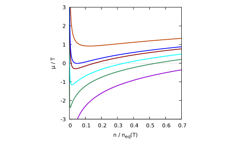
Figure 1: The generic function $g(x)=\ln x+\lambda x^{-1/3}$ for the scaled non-equilibrium chemical potential, $\mu/T$, as a function of the scaled particle number density, $n/n_{{\rm eq,id}}(T)$. Various values of $\lambda$ from the bottom to the top line are $0,0.5,0.75,1.0,1.1,1.5$.

Interesting enough, that in the Boltzmann approximation, where $n_{{\rm eq,id}}(T)=T^{3}/\pi^{2}$ for each degree of freedom, and counting with the traditional $37$ effective light degrees of freedom for a QGP we obtain the result that

$$T_{{\rm QGP}}\geq\frac{\sqrt{2}}{3}\,\frac{e^{1/2}\pi^{1/3}}{37^{1/6}}\,\sqrt{\sigma}\>\approx\>0.623\,\sqrt{\sigma}.$$ (10)

This result is near to the one obtained from early studies of the static quark – antiquark potential for the relation between the string tension and the color deconfinement temperature in pure lattice gauge theories STRINGTENSION1 ; STRINGTENSION2 ; STRINGTENSION3 ; STRINGTENSION4 . This very simple-minded model can also be extended to finite baryochemical potentials, and does perform appreciably STRINGY3 .

3 High-T effective field theory

It is known since long, already from the perturbative QCD treatment of the quark-gluon plasma (QGP) that interactions play a decisive role, and the description of equation of state at high temperature cannot be based solely on the model of an ideal gas of bare quarks and gluons. The more interesting that it can be and for a long time was being based on the ideal gas picture of quasiparticles, featuring the same number of degrees of freedom as colored elementary quarks and gluons do. The most prominent effect of interaction is concentrated to effective masses and its recursive effects on the pressure, energy density and entropy density at a given temperature.

First experiences on nontrivial problems in the non-interacting quasiparticle treatment arose from the study of the propagation of oscillatory excitations, so called plasmons, in hot QGP: original calculations on the gluon damping coefficient, which determines the speed of thermalization of a QGP, seemed to depend on the gauge fixing choice. Even its sign was disputed in the beginning UKT1987 ; GAUGEDEP1 ; GAUGEDEP2 ; GAUGEDEP3 .

The solution was found by Rob Pisarski and Eric Braaten with a resummation procedure of the so called hard thermal loops (HTL-s) HTL1 ; HTL2 ; HTL3 ; HTL4 ; HTL5 ; HTL6 ; HTL7 . The basis of this approach is a division of elementary quanta according to their momenta: ’hard’ are the hot thermal ones ($k\sim T$) and ’soft’ are at momentum scales characteristic to the interaction ($k\sim gT$ to leading order). Infinitely many Feynman graphs are grouped together so that the damping rate and the effective mass (self energy in the infrared limit) can be calculated with methods familiar from perturbative QCD. At high temperature the expansion according to the coupling strength, $g$, and according to the number of loops in Feynman diagrams, $\hbar$, is no more equivalent.

This, albeit is a big step forwards, does not solve alone all the problems. Most prominently the static magnetic gluon mass is of order $g^{2}T$, occurs at a ’supersoft’ scale, and cannot be generated by HTL resummation techniques alone. One considers e.g. a dilute magnetic monopole gas, whose density is proportional to $n\sim m^{3}\sim(g^{2}T)^{3}$, making a contribution to pressure and energy density at the level of $p\sim nT\sim g^{6}T^{4}$. In the perturbative QCD approach this term is related to an infrared divergence LINDE ; INFRA , and as such it is independent of UV renormalization schemes. The magnetic gluon mass of order $g^{2}T$ seems to be of genuine nonperturbative origin MAGMASS ; MAGMASS2 . It plays a role also in the calculation of other physically relevant quantities, like shear viscosity. Lattice QCD calculations on the other hand obtained this static magnetic gluon mass via observing a reduced dimensional string tension for space–space like Wilson loops as well as hunting for magnetic monopole looking configurations during the Monte-Carlo integration MONO1 ; MONO2 ; MONO3 ; MONO4 ; MONO5 ; MONO6 .

Basic formulas of high-temperature field theory make it possible to obtain order of magnitude estimates by assuming different dominant gluon field configurations, which contribute to the Euclidean path integral integrating the factors $\exp({iS/\hbar})$ with the action

$$S_{4}=i\int_{0}^{\hbar\beta}\limits\!d\tau\,\int\!d^{3}x\,\frac{1}{2}\left(E_{ia}^{2}+B_{ia}^{2}\right).$$ (11)

Here the chromoelectric field is related to the vector potential via the Euclidean time derivative, $E_{ia}=-\partial A_{ia}/\partial\tau$. The quantum theoretical path integral,

$$Z={\rm Tr}\left(e^{\frac{i}{\hbar}S_{4}}\right)\>=\>{\rm Tr}\left(e^{-\frac{1}{\hbar}\int_{0}^{\beta\hbar}\limits Hd\tau}\right),$$ (12)

is carried out for (with their gauge equivalent) $\tau$-periodic $A_{ia}$ fields with period $\beta\hbar$, and can therefore be reduced to a 3-dimensional partition sum at high temperature (small $\beta\hbar$):

$$Z_{3}\>=\>{\rm Tr}\left(e^{-\beta H}\right)$$ (13)

with

$$H_{3}\>=\>\frac{1}{2}\int\!d^{3}x\,\left(E_{ia}^{2}+B_{ia}^{2}\right).$$ (14)

In obtaining this result one assumes a constant $H(\tau)$ function in the narrow interval $(0,\beta\hbar)$. This is relevant in the study of the infrared behavior of the full, interacting theory.

For the sake of simplicity let us consider pure Yang-Mills theory (i.e. QCD without quarks) for a while. The path integral trace is over vector potential configurations, these can be re-scaled by the interaction strength: $gA\rightarrow A$ transformation leads to an effective, reduced 3-dimensional action with an effective coupling of the static magnetic mass

$$S_{3}\>=\>\frac{1}{g^{2}T}\,\int\!d^{3}x\,\frac{1}{2}B_{ia}^{2},$$ (15)

revealing the sought finite temperature partition sum as

$$Z_{3}\>=\>{\rm Tr}\left(e^{-S_{3}}\right).$$ (16)

Since this formula does not contain the Planck constant any more, we may confirm that the chromo-magnetostatic features of QGP can be estimated by purely classical field theory means. At the same time they are genuinely non-perturbative.

In the followings we review a few assumed gluon field configurations and investigate the corresponding mass and density scales of gluons, in the original setting, before re-scaling the vector potential with $g$. As a starting point we have to relate the magnitudes of the vector potential and that of the chromoelectric fields. We do this remembering that they are represented by canonically conjugate operators, satisfying

$$\left[E_{ia}(\vec{x}),\>A_{jb}(\vec{x})\right]\>=\>\frac{\hbar}{i}\,\delta_{ij}\,\delta_{ab}\,\delta(\vec{x}-\vec{y}).$$ (17)

Looking for quantum states possibly near to classical fields one singles out coherent states, where the Heisenberg uncertainty between the canonical operators is minimal.
Henceforth we use the intuitive estimate

$$E\cdot A\sim\hbar/L^{3},$$ (18)

assuming a quantization box of length $L$. We classify the gluon field configurations according to the magnitude of the vector potential and distinguish the following three fiducial classes:

1. The vector potential is large, of classical order (independent of $\hbar$): $A\sim 1/gL$. In this case $E\sim g\hbar/L^{2}$ and the magnetic field strength becomes $B\sim A/L+gA^{2}\sim 1/gL^{2}$, also classical. It receives Abelian and non-Abelian contributions in equal magnitude. The field energy,

   $$H=\frac{1}{2}\int\!d^{3}x\,(E^{2}+B^{2})\>\sim\>\frac{1}{g^{2}L}\,\left(\,1+{\cal O}\left((g^{2}\hbar)^{2}\right)\,\right),$$ (19)

   is also classical and dominated by the magnetic contribution for $g^{2}\hbar\ll 1$. Equating this value with the thermal gluon energy, $H\sim T$, we obtain the relation $1/L\sim g^{2}T$, i.e. the supersoft magnetic scale determines these configurations. The gluon density is estimated as being $n\sim 1/L^{3}\sim(g^{2}T)^{3}$ and the magnetic screening mass, the gluon self energy in the infrared limit, is estimated from $m^{2}A^{2}\sim g^{2}A^{4}$:

   $$m^{2}\sim g^{2}A^{2}\>\sim\>(g^{2}T)^{2}.$$ (20)

   This tour de force in estimates ends up with the mass $m\sim g^{2}T$.

2. The vector potential and the electric field strength share the quantum order but they are independent of the coupling, $g$. In this case one typically deals with configurations of $A\sim\sqrt{\hbar}/L$ and $E\sim\sqrt{\hbar}/L^{2}$. The magnetic field is Abelian dominated, $B\sim A/L+gA^{2}\sim\sqrt{\hbar}/L^{2}+g\hbar/L^{2}$. The dominant chromomagnetic field is of the same magnitude as the chromoelectric one. This describes a thermal state with equipartition and the energy density

   $$\varepsilon\sim\frac{T}{L^{3}}\>\sim\>\frac{\hbar}{L^{4}}.$$ (21)

   The characteristic scale from this is obtained as the thermal wavelength, $L\sim\hbar/T$, and the effective screening mass becomes

   $$m^{2}\sim g^{2}A^{2}\>\sim\>\frac{g^{2}T^{2}}{\hbar}.$$ (22)

   This Debye screening mass is of the order $m\sim gT/\sqrt{\hbar}$.

3. In principle a third class of configurations exists dominated by the classical chromoelectric field on the account of a vector potential of highly quantum order: $E\sim 1/gL^{2}$ and $A\sim g\hbar/L$. Physically this corresponds to the string picture and implies $E\gg A/L$ for $g^{2}\hbar\ll 1$. The Abelian part of the chromomagnetic field, $B_{Abel}\sim A/L\sim g\hbar/L^{2}\sim g^{2}\hbar E$ is then smaller than the chromoelectric field, while the non-Abelian contribution, $B_{non-Abel}\sim gA^{2}\sim g^{3}\hbar^{2}/L^{2}$ is even smaller, negligible in the semiclassical weak coupling approach. It is interesting that the thermal energy, dominated by the classical chromoelectric field,

   $$\varepsilon\>\sim\>\frac{T}{L^{3}}\>\sim\>\frac{1}{g^{2}L^{4}},$$ (23)

   again delivers a characteristic length scale of $L\sim 1/g^{2}T$. The screening mass effect, however, in this case is very small and of highly quantum nature:

   $$m^{2}\sim g^{2}A^{2}\>\sim\>\frac{g^{4}\hbar^{2}}{L^{2}},$$ (24)

   delivering at the end a mass scale of $m\sim g^{2}\hbar\cdot g^{2}T$.

Considering quasiparticles their mass is defined by the dispersion relation reflecting the Schwinger-Dyson equation with a general, complex self-energy

$$\omega^{2}-\vec{k}^{2}-\Sigma(\omega,\vec{k})\>=\>0.$$ (25)

Interacting with a medium during propagation is included in the general self-energy term, $\Sigma$. The resolution of eq.(25) for $\omega$ can also deliver complex values, the imaginary part of the frequency signalizes the so called plasmon damping. In the infrared limit, $|\vec{k}|\to 0$ the general frequency is $\omega+i\gamma$, satisfying

$$\left(\omega+i\gamma\right)^{2}\>=\>\Sigma(\omega+i\gamma,0).$$ (26)

In the weak damping limit, $\gamma\ll\omega$ the imaginary part of this equation defines

$$\gamma\>\approx\>\frac{1}{2\omega}\,\,\mathfrak{Im}\,\Sigma(\omega,0),$$ (27)

and the real part constitutes a mass gap equation

$$\omega^{2}\>\approx\>\,\mathfrak{Re}\,\Sigma(\omega,0).$$ (28)

To leading order in the perturbative expansion $\,\mathfrak{Re}\,\Sigma(\omega,0)=(m/\hbar)^{2}$ with $m$ being the mass scale derived above. With $\omega\sim T/\hbar$ taken as hard thermal, the weak damping constant becomes $\gamma\sim m^{2}/\hbar T$. This is perturbatively the largest in the second class, $\gamma_{2}\sim g^{2}T/\hbar$.

4 Internal Structure of QGP

The fact that QCD is a strongly interacting theory changes several concepts originally stemming from the free particle world.

4.1 Particles in strongly interacting system

In an interacting field theory the notion of a “particle” needs careful definition. The problem is that the concept of a “particle” is associated with free field theory; but, in fact, there are various definitions that refer to the same physical phenomenon in non-interacting theories, any of them being appropriate to describe a free particle:

• In free theory there exists a conserved particle number operator $\hat{N}$ that also commutes with the momentum operator, too. The common eigenvectors of the energy, momentum and particle number in the $N=1$ sector are the free particles. The $N>1$ sector consist of direct products of one-particle states; the direct sum of all $N$-particle sectors provides the Fock-space construction.

• The energy $E$ and momentum $k$ of a free one-particle state is connected by the dispersion relation $E=E(\bm{k})$. Therefore the spectrum of the one-particle sector consists of a single energy level, let us denote it $\left|E,\bm{k}\right\rangle$. The spectral density of this sector is therefore a single Dirac-delta. To measure the spectral density we can use any operator $\hat{\Phi}$ that posesses only a one-particle form factor, ie. $\langle E,\bm{k}|\hat{\Phi}|0\rangle\neq 0$, but $\langle E,\bm{k};E^{\prime},\bm{k}^{\prime}|\hat{\Phi}|0\rangle=0$. Then we define

  $$\varrho(t)=\langle 0|[\hat{\Phi}(t),\hat{\Phi}(0)]_{\pm}|0\rangle,$$ (29)

  where $\pm$ refers to the commutator/anticommutator, depending on the bosonic/fermionic nature of the particles. In Fourier space this definition is equivalent with a weighted spectral density

  $$\varrho(\omega)=\sum_{E,\bm{k}}\left|\langle E,\bm{k}|\hat{\Phi}|0\rangle\right|^{2}2\pi\delta(\omega-E(\bm{k})).$$ (30)

  In a relativistic field theory, using the fundamental field as a measurement operator we have the spectral function

  $$\varrho(\omega,\bm{k})=\frac{2\pi}{2E(\bm{k})}\left[\delta(\omega-E(\bm{k}))-\delta(\omega+E(\bm{k}))\right].$$ (31)

  This satisfies the sum rule

  $$\int\frac{d\omega}{2\pi}\omega\varrho(\omega,\bm{k})=1,$$ (32)

• The spectral function remains unchanged at finite temperature, so a particle at finite temperature is the same object as a zero temperature particle.

• As a consequence the wave function of the free particle is $\Psi(t,\bm{x})\sim e^{-iEt+i\bm{kx}}$, an infinite extension plane-wave, with $|\Psi|^{2}=1$ uniform probability density.

• The linear response to a disturbance leads to the linear response function, or retarded Green’s function. The retarded Green’s function reads as

  $$G_{ret}(\omega,\bm{k})=\frac{1}{(\omega+i\varepsilon)^{2}-E^{2}(\bm{k})}$$ (33)

  in relativistic systems. This form is preserved at finite temperature.

In free theory these all are consequences of each other, therefore we unintentionally identify these concepts, and when we tell “particle”, it means all of these at the same time.

However, in an interacting model all of these concepts yield different results, and so we have to release the identification of the above concepts.

• In a general field theory the number of conserved quantities is much smaller than the number of state labels (types of quantizable physical degrees of freedom); the only exceptions are integrable systems. In particular the particle number operator does not exists any more.

• We can measure the spectral function in the same way as we did in the free case. But, because of the interactions, the spectrum of the free one-particle states will be mixed with the spectrum of the higher particle number states. These will provide a continuum contribution besides the free particle state. Since the spectrum is subject of a sum rule, cf. (32), the height of the Dirac-delta peak can not be the free one, it receives a multiplicative correction $Z$ (wave function renormalization).

• The spectrum is more complicated at finite temperature or at finite chemical potential: there the spectral function is nonzero for all frequencies (with the sole exception $\omega=0$), as a consequence of the scattering on particles in the environment. This broadens the Dirac-delta particle peak, resulting in a Lorentzian curve. Such an excitation is called quasiparticle. It, as opposed to the free case, does not represent a single energy level, but a collection of energy eigenstates. Here other excited/ground states can appear too, and the continuum is always present. A typical finite temperature spectrum can be seen on Fig. 2.

  

  Figure 2: Typical spectrum in an interacting theory. The original particle peak is broadened (finite lifetime or finite coherence length), other peaks can appear (excited and bound states), moreover we always have a multi-particle continuum contribution.

• The linear response function at zero temperature still contains contribution from the Dirac-delta peak. For long times we obtain

  $$G_{ret}(t,\bm{k})=Ze^{-iE(\bm{k})t}+Ct^{-3/2}e^{-iE_{thr}(\bm{k})t}+\dots.$$ (34)

  For long times the second part dies out, leaving a free particle like propagation: these are the asymptotic states.

• In numerous cases, however, there are no asymptotic states: if the particle mixes with zero mass particles (all charged particles do that), or the particle is not stable, or we are at nonzero temperature; practically in all realistic cases. The Lorentzian quasiparticle peak and the continuum part of the spectral function yield the retarded propagator

  $$G_{ret}(t,\bm{k})=Ze^{-iE(\bm{k})t-\gamma_{\bm{k}}t}+Ct^{-3/2}e^{-iE_{thr}(\bm{k})t-\Gamma_{\bm{k}}t}+\dots.$$ (35)

  where $\gamma_{\bm{k}}$ is the half-width of the Lorentzian peak, and $\Gamma_{\bm{k}}$ is some parameter determining the smoothing of the spectrum near the threshold. The quasiparticles for long times decay exponentially. If $\gamma_{\bm{k}}\ll\Gamma_{\bm{k}}$, for long times we can observe a fading quasiparticle response, in the reverse case, $\gamma_{\bm{k}}\gg\Gamma_{\bm{k}}$, the long time behavior of the system is not particle-like at all.

Having said all these we see that the particle concept becomes a dangerous ground, we must be very precise on what we are talking about. For example stating that the particles have temperature dependent mass is sensible only in the quasiparticle-sense: free particles are eigenstates of the Hamiltonian, they cannot have a mass changing with the temperature. The quasiparticles, on the other hand, are collections of energy eigenstates, and the coefficients of the combination can change with $T$. Therefore the position and the width of the quasiparticle peak can also change with the temperature.

4.2 Particles, spectral function and thermodynamics

There is still a possible definition for a particle through thermodynamics: in free theory each particle species represents a thermodynamic degree of freedom. Does it remain true in the interacting case, i.e. are also the nonperturbative particle species thermodynamic degrees of freedom? Let us seek an answer to this question by utilizing spectral properties.

The pressure of the free gas of different species is the sum of partial pressures $P=\sum_{n}P_{n}$ with

$$P_{n}=\mp\frac{T^{4}}{2\pi^{2}}\int\limits_{0}^{\infty}\!dx\,x^{2}\ln(1\mp e^{-\sqrt{x^{2}+(\beta m_{n})^{2}}}),$$ (36)

where $m_{n}$ is the mass of the $n$th particle, and $\mp$ refers to the bosonic/fermionic case, respectively. In particular the pressure at large temperature, in the Stefan-Boltzmann limit, $T\gg m$, reads as

$$P_{free}=\frac{\pi^{2}}{90}\left(N_{b}+\frac{7}{8}N_{f}\right),$$ (37)

where $N_{b}$ is the number of bosonic, $N_{f}$ the number of fermionic species. All fundamental free particles therefore contribute independently to the pressure.

We do not need to have, however, fundamental particles to obtain thermodynamical degrees of freedom. In the case of well separated quasiparticle excitations, that can be characterized by a phase shift $\delta(\omega)$ of a scattered particle centered at $\omega=E(\bm{k})$, the Beth-Uhlenbeck formula Landau states

$$\delta Z\sim\int\limits_{0}^{\infty}\frac{d\omega}{2\pi}\frac{\partial\delta}{\partial\omega}e^{-\beta\omega}\sim e^{-\beta E(\bm{k})}.$$ (38)

Therefore all excitations contribute to the partition function exactly like a stable particle, irrespective whether it is a fundamental particle, or a bound state with internal structure and motion.

This picture leads to the Hadron Resonance Gas (HRG) description of the QCD plasma HRG0 . Here all the possible hadrons, measured and identified at zero temperature, contribute to the thermal ensemble in the same way, irrespective of their width. The resulting pressure is in fact in a very good agreement with the pressure measured in MC simulations in the hadronic phase Andronic:2003 ; Karschetal ; Huovinen:2009yb ; Borsanyi:2010cj ; Bazavov:2013dta .

It fails, however, badly in the quark-gluon phase, about $T>150$ MeV Bazavov:2013dta ; FLUKARS4 . In fact, as it was first pointed out by Hagedorn, the HRG pressure would be divergent, if all hadrons were taken into account. This is due to the fact that the density of hadron states grows exponentially with the mass: $\rho(m)\sim m^{\alpha}e^{\beta_{H}m}$, with $T_{H}=1/\beta_{H}$ Hagedorn temperature, and an appropriate power $\alpha$ (e.g. $\alpha=5/2$). Then the pressure of all hadrons, written up as an integral for the mass density diverges,

$$P\sim\int\!\!dm\,\rho(m)\,e^{-\beta m}\>\to\>\infty,\qquad\mathrm{for}\qquad T>T_{H}.$$ (39)

If we do not take into account all hadrons, just those that are listed in the Particle Data Book PDG , or the hadrons below, say 3 GeV, then the pressure will not diverge, but still overshoots the pressure of the quark gluon plasma. This is a conceptual problem: at all temperatures the system in equilibrium realizes that phase where the grand-canonical thermodynamical potential, in this case $PV$, is the largest. The quark gluon plasma with 8 gluons and $N_{f}$ quarks represents a system with $16+10.5N_{f}$ bosonic degrees of freedom (all fermions have 4 Lorentz-components, 3 colors, and the factor $7/8$ compared to the bosonic contribution). If we would count only the stable hadrons, i.e. pions and nucleons, as hadronic degrees of freedom, we would obtain $10$ bosonic degrees of freedom, and so the QGP would have a larger number of degrees of freedom, which explains, why there is a phase transition to the QGP phase. But if all the Particle Data Book hadrons are taken into account, this highly exceeds the QGP number of degrees of freedom, and we do not understand, why a phase transition occurs at all? We must emphasize that the argument that the hadrons are not valid degrees of freedom in the QGP phase is not applicable, since the hadron phase represents a higher entropy state of matter, and so it forbids the change to the QGP phase.

So we are faced with the situation, where we can describe the pressure of the strongly interacting plasma below $\sim 150$ MeV (HRG), and above $300$ MeV (QGP), but we do not understand why there is a phase transition, and we do not understand the pressure in the intermediate temperature range. What happens with the hadrons between $150\,\mathrm{MeV}<T<300\,\mathrm{MeV}$? The bound states must somehow disappear from the system as we rise the temperature, physically the hadrons must melt away.

How is this melting related to the Beth-Uhlenbeck formula, according to that every quasiparticle resonance corresponds to a single thermodynamical degree of freedom? We should note that in the derivation of the result one must assume that the quasiparticles are independent, in the sense that all can be treated as separate Breit-Wigner peaks. This assumption, however, fails when we consider a system where the quasiparticle peaks occur densely, or if a multiparticle background is present. In such cases the quantum mechanical treatment of the quasiparticle peak contributions to the $S$ matrix have complex coefficients Scon ; Svec . The unitarity of the $S$ matrix poses constraints among these coefficients: in this way the pole contributions are no more independent.

In field theory we can describe this process by observing the hadronic spectral functions Jakovac:2012tn ; Jakovac:2013iua ; ALLCONFB . A mathematically similar description can be obtained using the Mott-transition analogy Turko:2011gw ; Benic:2013tga ; Blaschke:2015nma . The hadronic spectral functions, as all spectral functions, consist of a quasiparticle peak and a continuum part. The weight of these parts, however, changes with the temperature. At small temperatures the quasiparticle peak is pronounced, it dominates the thermodynamics, and the gas of hadrons behaves as a gas of almost free particles. At high temperatures, however, the quasiparticle peak merges with the continuum, and the “particle” nature of the hadronic channel ceases to be true. This is accompanied by a drastic reduction of the partial pressure in this channel.

To set up a field theoretical model we construct a quadratic theory with the same statistical property (boson/fermion) and the same spectral function as the studied channel. For a scalar field it means that we write up the Lagrangian as

$${\cal L}\>=\>\frac{1}{2}\Phi\,{\cal K}(i\partial)\,\Phi,$$ (40)

with some kernel ${\cal K}$. The kernel and the retarded Green’s function are related as $G_{ret}(p)={\cal K}^{-1}(p_{0}+i\varepsilon,\bm{p})$, while the retarded Green’s function and the spectral function can be expressed from each other

$$G_{ret}(p)\>=\>\int\limits_{-\infty}^{\infty}\!\frac{d\omega}{2\pi}\frac{\varrho(\omega,\bm{p})}{p_{0}-\omega+i\varepsilon},\quad\varrho(p)=\mathop{\mathrm{Disc}}_{p_{0}}iG_{ret}(p).$$ (41)

Since the theory described by the effective Lagrangian (40) is quadratic, and so it is solvable; but its spectrum does not consists of free particles. To determine thermodynamics one has to start from a microscopically measurable quantity, which most conveniently can be chosen the energy density, ie. the expectation value of the 00 component of the energy-momentum tensor $T_{00}$. Although we have a quadratic, model, the energy-momentum tensor is not simple, due to the nonlocal nature of the kernel. The divergence of the energy-momentum tensor can be determined from the variation of the action with respect to a space-time translation $a_{\mu}$ Collins

$$\partial^{\mu}T_{\mu\nu}=\frac{\delta S}{\delta a^{\mu}}.$$ (42)

This leads to Jakovac:2012tn

$$T_{\mu\nu}(x)=\frac{1}{2}\Phi(x)\,D_{\mu\nu}{\cal K}(i\partial)\,\Phi(x)$$ (43)

where

$$D_{\mu\nu}{\cal K}(i\partial)=\left[\frac{\partial{\cal K}(p)}{\partial p^{\mu}}\biggr{|}_{p\to i\partial}\right]_{sym}\!\!\!i\partial_{\nu}-g_{\mu\nu}{\cal K}(i\partial),$$ (44)

and the symmetrized derivative is defined as

$$f(x)[(i\partial)^{n}]_{sym}g(x)=\frac{1}{n+1}\sum\limits_{a=0}^{n}[(-i\partial)^{a}f(x)][(i\partial)^{n-a}g(x)].$$ (45)

Once we know $T_{\mu\nu}$, wa can take its expectation value in equilibrium. We can use KMS relation to write

$$\left\langle\Phi(x)\Phi(y)\right\rangle=\int\!\frac{d^{4}p}{(2\pi)^{4}}e^{-ip(x-y)}\left(\frac{1}{2}+n(p_{0})\right)\varrho(p).$$ (46)

Finally we renormalize the expressions and express pressure through thermodynamical relations. The result reads Jakovac:2012tn ; Jakovac:2013iua ; ALLCONFB

$$P=\mp T\int\!\frac{d^{4}p}{(2\pi)^{4}}\,\Theta(p_{0})\frac{\partial{\cal K}}{\partial p_{0}}\varrho(p)\ln(1\mp e^{-\beta p_{0}}).$$ (47)

We should note that the pressure does not depend on the normalization of the spectral function, since the kernel is inversely proportional to this normalization factor (cf. (41)).

In the free case, ie. using the free spectral function (31) and ${\cal K}=p^{2}-m^{2}$ in the above formula, we get back the free pressure (36). If there are several Dirac-delta peaks in the spectrum, we also get back the sum of the free gas partial pressures, in accordance with the Beth-Uhlenbeck formula (38). But if the peaks are not independent, the exact pressure starts to deviate from the Beth-Uhlenbeck prediction. In Fig. 3 we can see that when two peaks start to merge, the exact pressure decreases.

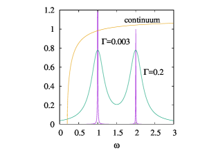
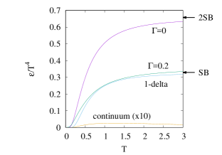
Figure 3: Left panel: spectral functions of two peaks with different widths as well as a pure continuum. Right panel: energy density of two peaks with different widths, the energy density of a single Dirac-delta peak (with $m=1.6$), and the energy density contribution of the continuum, enlarged by a factor of 10

It is not unexpected: when there is just one peak, the spectrum looks like a one-quasiparticle spectrum, and so the pressure must come from a single degree of freedom. Therefore starting from a two separate peaks spectrum, and continuously approach a one-peak spectrum the pressure also changes smoothly from the two-particle pressure to the one particle one.

This observation leads to the explanation of Gibbs-paradox in interacting systems Jakovac:2012tn . The original paradox, valid in free systems is that if the molecules of two gases differ only in a tiny, continuously disappearing thing (eg. mass difference, or a tiny “flag”), then the two gases are different as long as the difference is present, but are the same if the difference is exactly zero. This leads to a non-analytic contribution to the entropy (mixing entropy). In interacting gases, however, the energy spectrum consists not infinitely thin Dirac-deltas, but there is a line broadening coming from different sources (eg. thermal motion, or finite density). Then with vanishing mass difference the spectral functions become more and more overlapping, as it is shown in Fig. 3. As a consequence the pressure will continuously reduce from the 2-independent particle pressure to a 1-particle pressure (where the mass is somewhere between the masses of the two peaks), as it is also shown in Fig. 3. In an interacting system, therefore, the Gibbs-paradox leads to a continuously vanishing mixing entropy.

In Fig. 3 there is shown also the contribution of the multiparticle continuum (cut) part. Its spectrum is not quasiparticle-like, as it can be seen on the left panel of Fig. 3. The corresponding pressure is much lower than the pressure of the quasiparticle systems: in Fig. 3 it is enlarged by a factor of 10 to be visible at all.

This explains why a huge pressure reduction appears when a peak merges with the continuum, ie. when it melts. The original narrow peak structure corresponds to an almost free quasiparticle, with pressure close to the free pressure. When the peak gets merged in the continuum, the spectrum does not contain a particle, it becomes more and more like the continuum part of Fig. 3, therefore the corresponding pressure is also smaller and smaller. In the course of a continuous merging procedure the pressure smoothly changes from the one free particle pressure to zero: the particle is melted, it disappears from the thermal ensemble. We can define the number of thermodynamical degree of freedom as the ratio of the exact pressure and the free pressure. With this definition the thermodynamical degrees of freedom changes continuously to zero.

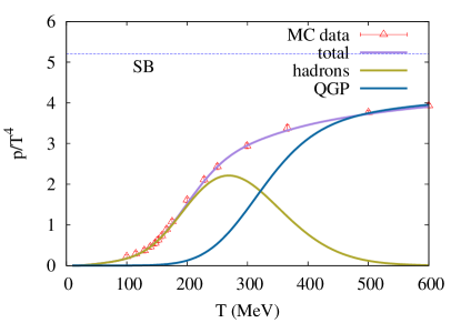
Figure 4: Hadronic pressure reduction at high $T$, quark pressure reduction at low $T$, due to merging peaks. For comparison, lattice data are indicated by triangles.

This mechanism makes it possible to explain why there is no divergent pressure beyond the Hagedorn temperature in the QCD plasma, or why the hadronic pressure does not overshoot the QGP pressure. The hadron spectrum changes with the temperature from quasiparticle peaks to peaks merged with the continuum. As discussed above, this results in the reduction of the thermodynamical degrees of freedom effective for the total pressure. The situation is just the opposite for the QGP degrees of freedom: at small temperatures the spectrum in the quark channel is just a continuum, there are no particle-like excitations there, the partial pressure is zero. At high temperatures the spectra in the QGP channels become more and more particle-like; although even at about $T\approx 300$ MeV the number of thermodynamical degrees of freedom is only about 80% of the free case (cf. Fig.4).

In this way, within the picture of melting quasiparticle peaks, the QCD pressure computed in MC simulations can be reproduced and interpreted in correct physical terms. The main prediction of this model is that the hadronic thermodynamic degrees of freedom do not vanish suddenly above the critical temperature, there is a sizable temperature regime, until about $T=330$ MeV, where they still dominate the pressure. In this melting hadron peak regime, however, we do not have quasiparticles as excitations, just a mixture of hadron-like and dissociated quark-gluon-like behavior. This is indeed a new type of nuclear matter.

4.3 Continuous mass fits to lattice EoS

Quark matter, searched for in relativistic heavy ion collisions, reveals itself in signatures on observed hadron spectra which are interpreted in terms of quark level properties. In particular scaling of the elliptic flow component $v_{2}$ with the constituent quark content of the finally observed mesons and baryons v2 ; v2B ; v2C ; v2D ; v2E ; v2F and successful description of $p_{T}$-spectra of pions and antiprotons using quark coalescence rules for hadron building ourJPG utilize the fast hadronization concept of quark redistribution. Albeit this simple idea brings also problems with it, e.g. in dealing with energy conservation and entropy increase, these issues can be resolved by using a distributed mass quasiparticle model for quark matter ourPRChep , and are in accord with the quark matter equation of state obtained in lattice QCD calculations ourPLB . The surmised mass distribution gives rise to specific equation of state (pressure as a function of temperature, $p(T)$), and reversed, a mass distribution may be outlined from knowledge on the $p(T)$ curve.

While traditional, fixed mass quasiparticle models already succeed to describe the equation of state obtained in lattice QCD Quasiptl , those mass values are themselves temperature dependent. Furthermore a temperature dependent width is associated to the quasiparticle mass, too Quasi2 ; Quasi3 ; Peshier . The factor between the massive and massless relativistic ideal pressure in the Boltzmann approximation,

$$\Phi\left(\frac{m}{T}\right)\>=\>\frac{p_{{\rm id}}(m,T)}{p_{{\rm id}}(0,T)}\>=\>\frac{1}{2}\,\frac{m^{2}}{T^{2}}\,K_{2}\!\left(\frac{m}{T}\right),$$ (48)

relates the observed pressure in a non-trivially interacting system to the mass distribution of a conjectured continuous mixture of different mass particles

$$p(T)\>=\>\int_{0}^{\infty}\limits\,\!w(m)\,p_{{\rm id}}(m,T)\,dm.$$ (49)

This means that the observed equation of state in terms of the pressure ratio to the Stefan–Boltzmann limit, representing the effective fraction of thermodynamical degrees of freedom, is a so called Meijer transform of a conjectured continuous mass distribution:

$$\sigma(T)\>=\>\frac{p(T)}{p_{{\rm id}}(0,T)}\>=\>\int_{0}^{\infty}\limits\,\!\!w(m)\,\frac{1}{2}\,\frac{m^{2}}{T^{2}}\,K_{2}\!\left(\frac{m}{T}\right)\,dm.$$ (50)

Using the scaled variables, $t=m/T_{c}$ and $z=T_{c}/T$, and the redefined functions $\sigma(z):=\sigma(T_{c}/z)$, $w(t):=T_{c}w(T_{c}t)$, we obtain

$$\sigma(z)\>=\>\int_{0}^{\infty}\limits\,\!\!w(t)\,\frac{z^{2}t^{2}}{2}\,K_{2}\!\left(zt\right)\,dt.$$ (51)

This integral transformation, the so called Meijer transform, can be inverted analytically,

$$w(t)\>=\>\frac{2}{i\pi}\int\sigma(z)\,\frac{I_{2}(zt)}{zt}\,dz.$$ (52)

The respective high temperature expansions of the pressure ratios, based on the expansion of the $K_{2}(z)$ Bessel function in the mass distribution formula, and that one applied in perturbative QCD, are worth to be compared:

$$\frac{p(T)}{p_{{\rm id}}(0,T)} = 1-\frac{\langle{m^{2}}\rangle}{4T^{2}}+\left(\frac{3}{4}-\gamma\right)\frac{\langle{m^{4}}\rangle}{16T^{4}}$$

$$+\,\frac{\langle{m^{4}\ln(2T/m)}\rangle}{16T^{4}}+\ldots,$$

$$\frac{p_{{\rm pQCD}}}{p_{{\rm id}}(0,T)} = 1-a_{2}g^{2}+a_{4}g^{4}+b_{4}g^{4}\ln\frac{2\pi T}{\Lambda}+\ldots$$ (53)

with $\gamma$ being the Euler–Mascheroni constant and $\Lambda$ the renormalization subtraction scale. We note that $\sigma(z)$ can also be obtained for Bose or Fermi distributions instead of the Boltzmann one; the numerical difference is overall minor, less than six per cent at vanishing chemical potential. The basic result on the Debye screening length in a QGP supports the assumption that $\left\langle{\>m^{2}\>}\right\rangle\sim g^{2}T^{2}$ sets the scale for a simplified treatment of the quark matter pressure at high temperature. The comparison of pQCD and mass distribution results above reveals that $\left\langle{\>m^{4}\>}\right\rangle\neq\left\langle{\>m^{2}\>}\right\rangle^{2}$, whence the necessity of a width in the mass distribution emerges. Alone this fact indicates that the spectral function cannot be a simple sum of quasiparticle peaks, it must contain appreciable widths, possibly even a continuum part.

The temperature dependence of the pressure ratio to the massless ideal gas value is concentrated on the temperature dependence of the coupling constant: $g=g(T)$ in the traditional interpretation. We have recently pursued an alternative approach to the quasiparticle mass distribution in quark matter ourJPG ; ourPRChep , where a temperature independent $w(m)$ distribution is reconstructed from the pressure ratio $\sigma(T)=p(T)/p_{{\rm id}}(0,T)$ curve:

$$\sigma(T)=\int_{0}^{\infty}w(m)\>\Phi\left(\frac{m}{T}\right)\,{\,\mathrm{d}}m.$$ (54)

It is interesting to play around with some analytic formulas with respect to the Meijer transformation. The simple exponential ansatz leads to a certain power-law tailed form of $w(m)$ with a threshold mass gap at $m=\lambda$:

$$\sigma(T)\>=\>\,\mathrm{e}^{-\lambda/T}\,\>\leftrightarrow\>w(m)\>=\>\frac{4\lambda}{\pi m^{2}}\,\sqrt{1-\frac{\lambda^{2}}{m^{2}}}.$$ (55)

Since such a mass distribution would have a diverging $\left\langle{\>m^{2}\>}\right\rangle$ and also for higher powers of $m$, we conclude that it must be

$$\sigma(T)\><\>\,\mathrm{e}^{-\lambda/T}\,.$$ (56)

Indeed lattice results on $\sigma(T)$ all satisfy such a constraint with a corresponding value of $\lambda$. The smallest such $\lambda$ value, found numerically, is then the Boltzmannian estimate for the mass gap. It is a remarkable property of this approach that it indicates a temperature independent threshold (smallest mass) in the $w(m)$ spectrum for lattice QCD pressure dataFODOR ; BIELEFELD .

The pressure is, however, not known analytically, the numerical results are smeared with error bars. This problem is more severe in the light of the fact that eq.(50) constitutes an integral transformation (the Meijer K transformation, a generalization of the Laplace transformation). There is no mathematical guarantee that the inverting transformation eq.(52) leads to close results for $w(m)$ from close functions for $\sigma(T)$. In fact this is known as the ”inverse imaging problem” IMAG ; IMAG2 ; IMAG3 .

However, based on the above assumptions one can obtain some supportive knowledge about a $T$-independent $w(m)$ mass distribution when the pressure $p(T)$ satisfies certain inequalities. In particular we prove that if the pressure $p(T)$ is below the corresponding ideal gas pressure with a given mass $M_{0}$ at all temperatures, then the mass distribution is exactly zero for all masses below $M_{0}$. For inequalities with other than ideal gas pressure curves as estimators we apply the Markov inequality for probability measures, which directly offers upper bounds on the integrated probability density function $P(M)=\int_{0}^{M}\limits w(m)dm$. It turns out that the appearance and value of the highest possible $M$ for which $P(M)=0$, the mass gap value $M_{0}$, is connected to the low temperature behavior of $\sigma(T)$. Two particular estimators for $\sigma(T)$, namely $\Phi(M_{0}/T)$ with $M_{0}=3.2T_{c}$ and $\exp(-T_{c}/T)$ are compared to 2+1 flavor lattice QCD scaled pressure data in Figure 5 (top) and to pure SU(3) lattice gauge theory data (bottom) with $M_{0}=2.7T_{c}$ and $\lambda=0.55T_{c}$. Of course the temperature scales are different, $T_{c}\approx 165$ MeV in the first, $T_{c}\approx 260$ MeV in the second case. These examples are important for gaining a physical insight into the Markov inequality discussed below.

Figure 5: Pressure curve estimators for the data from lattice QCD simulation of Ref.FODOR (2+1 flavor QCD) and of SU3 ; SU3B (pure SU(3) gauge theory).

In the followings we relate the mass gap to the behavior of $\sigma(T)$ using the generalized Markov inequality to estimate upper bounds on the integrated probability density function for the mass being lower than a given value. The general form of the Markov inequality is given by MARKOV1 ; MARKOV2 ; MARKOV3 ; MARKOV4

$$\mu\left(\left\{x\in X:f(x)\geq t\right\}\right)\leq\frac{1}{g(t)}\int\limits_{x\in X}g\left(\,f(x)\,\right){\,\mathrm{d}}\mu(x)$$ (57)

with measure $\mu$, a real valued $\mu$-measurable function $f$, and a monotonic growing non-negative measurable real function $g$. The proof, based on the monotonity of integration, can be presented in a few lines. For a non-negative and monotonic growing function $g(t)\leq g(f(x))$ for $t\leq f(x)$. We obtain

$$g(t)\!\!\!\!\!\!\int\limits_{f(x)\geq t}\!\!\!\!\!\!{\,\mathrm{d}}\mu(x)\>=\!\!\!\!\!\!\int\limits_{f(x)\geq t}\!\!\!\!g(t){\,\mathrm{d}}\mu(x)\>\leq\!\!\!\!\!\!\int\limits_{f(x)\geq t}\!\!\!\!g\left(\,f(x)\,\right){\,\mathrm{d}}\mu(x).$$ (58)

This quantity can be bounded by

$$\int\limits_{f(x)\geq t}g\left(\,f(x)\,\right){\,\mathrm{d}}\mu(x)\>\leq\>\int\limits_{x\in X}g\left(\,f(x)\,\right){\,\mathrm{d}}\mu(x).$$ (59)

A division by $g(t)\geq 0$ delivers the original statement in eq.(57).

In order to apply this inequality to the mass spectrum we choose $f(m)=tM/m$. In this case

$$\mu\left(\frac{tM}{m}\geq t\right)=\int_{0}^{M}{\,\mathrm{d}}\mu(m),$$ (60)

and the Markov inequality reads as

$$P(M):=\int_{0}^{M}{\,\mathrm{d}}\mu(m)\leq\frac{1}{g(t)}\int_{0}^{\infty}g\left(\frac{tM}{m}\right){\,\mathrm{d}}\mu(m).$$ (61)

For a continuum mass spectrum ${\,\mathrm{d}}\mu(m)=w(m){\,\mathrm{d}}m$ can be chosen with $w(m)$ being the probability density function. The generalized Markov inequality stated above is valid for general probability measures $\mu$ possibly including bound state contributions.

Now we discuss a few examples for monotonic rising functions $g(z)$, which allow us to draw some conclusions about the integrated probability for masses below $M$. Applying the special form of $g(t)=t^{n}$ we arrive at

$$P(M)\leq\frac{1}{t^{n}}\int_{0}^{\infty}\left(\frac{tM}{m}\right)^{n}w(m){\,\mathrm{d}}m,$$ (62)

whence we obtain:

$$P(M)\leq M^{n}\int_{0}^{\infty}m^{-n}w(m){\,\mathrm{d}}m.$$ (63)

It is easy to see that the negative integral moments of the mass on the right hand side of the above inequality are connected to the negative integral moments of scaled pressure $\sigma(T)=p(T)/p_{{\rm id}}(0,T)$. The final inequality for the probability of having masses smaller than $M$ is given by

$$P(M)\>\leq\>M^{n}\,\frac{\int_{0}^{\infty}\limits\,T^{-n-1}\,\sigma(T)\,{\,\mathrm{d}}T}{\int_{0}^{\infty}\limits\,x^{n-1}\,\Phi(x)\,{\,\mathrm{d}}x}.$$ (64)

Figure 6: Reconstructed scaled mass distribution using analytic (continuous line) and numerical Meijer back transformation (black boxes: lattice EoS data, black circles: exponential upper estimate) on the top. Upper bounds for the integrated probability $P(M)$ of masses lower than $M$, based on 2+1 flavor lattice QCD EoS dataFODOR at the bottom (cf. eq.68).

Let us apply this result to the simplest majorant, that of a fixed mass relativistic ideal gas. In this case $\sigma(T)\leq\Phi(M_{0}/T)$ with some $M_{0}$ (cf. dashed line in Figure 5). Equation (64) leads to

$$P(M)\>\leq\>M^{n}\frac{\int_{0}^{\infty}T^{-n-1}\,\Phi\!\left(\frac{M_{0}}{T}\right){\,\mathrm{d}}T}{\int_{0}^{\infty}x^{n-1}\Phi(x){\,\mathrm{d}}x}\>\leq\>\left(\frac{M}{M_{0}}\right)^{n}$$ (65)

in this case. Should it hold for arbitrary high $n$, the right hand side of this inequality is zero for all $M<M_{0}$ and divergent for $M>M_{0}$. In the second case it is not restrictive, since $P(M)<1$ anyway, in the first case this means a mass gap up to $M_{0}$. We note that this conclusion holds for a general non-negative $\Phi(x)$, for which the integrals in eq.(65) are finite for all $n>0$. Thus the Bose-Einstein or the Fermi-Dirac distribution could as well be applied instead of the Boltzmann one.

Another possible majorant is the exponential function, $\sigma(T)\leq\exp(-\lambda/T)$ (cf. the dotted line in Figure 5 for $\lambda=T_{c}$). In this case eq.(64) delivers

$$P(M)\leq\left(\frac{M}{2\lambda}\right)^{n}\frac{2\Gamma(n)}{\Gamma(2+n/2)\Gamma(n/2)}.$$ (66)

The large $n$ limit of this result is given by

$$P(M)\leq\left(\frac{M}{\lambda}\right)^{n}2\sqrt{\frac{2}{\pi}}\frac{1}{n^{3/2}}$$ (67)

to leading order in $1/n$. Again the right hand side approaches zero for $M\leq\lambda$ and diverges for $M>\lambda$. This points out a mass gap stretching to (and including) $\lambda$ from zero.

Figure 7: Upper bounds for the integrated probability of masses lower than $M$ based on eq.(69) and on 2+1 flavor lattice QCD EoS dataFODOR (top) and from Ref.BIELEFELD (bottom) respectively. The estimates belong to different temperatures $T$ near $T_{c}$ indicated in the legend. In the second case a constant error of $0.01$ was assumed in the original $p/T^{4}$ data.

The most striking inequality is obtained by using $g(t)=\Phi(1/t)$. This function is also admissible, its rise from zero to one is strict monotonic. Eq. (64) leads to

$$P(M)\>\leq\>\frac{\sigma(tM)}{\Phi(1/t)}.$$ (68)

For $t=1$ using the numerical value $\Phi(1)\approx 0.81$ one arrives at $P(M)\leq 1.23\sigma(M)$, which can be directly read off from numerical simulation or theoretical predictions of $\sigma(T)$. Figure 6 presents curves for different $t$-values (see legend), all being an upper estimate for the integrated probability $P(M)$ in the respective cases of 2+1 flavor QCD and pure SU(3) gauge theory. The higher seems to be the starting $M_{0}$ value for the rise of the upper bound on $P(M)$, the higher also the magnification of the error bars. A secure estimate for the $P(M)\leq 0.05$ is given for masses $M>1.7T_{c}=280$ MeV for the 2+1 flavor QCD case, while for $M>7.2T_{c}=1.9$ GeV for the pure SU(3) gauge case. While in the first case this can be at best an average between quark and gluon-like quasiparticle masses, in the second case should be close to observed glueball mass. We note that using $\sigma(tM)\leq\Phi(M_{0}/tM)$ in the $t\rightarrow 0$ limit again a mass gap at $M_{0}$ follows from eq.(68). In this respect the use of different $g(z)$ functions in the Markov inequality does not matter.

A related version of the inequality (68) is obtained for $tM=T$, $g(z)=\Phi(tM/zT)$. The upper bound is obtained at any fixed $T$ as being

$$P(M)\>\leq\>\frac{\sigma(T)}{\Phi(M/T)}$$ (69)

Figure 7 plots upper bounds for $P(M)$ obtained using the eq.(69). The most restrictive are the lowest temperature data for $\sigma(T)$, they are, however, also the most contaminated by errors. It is probably safe to conclude that as much as $90-95\%$ of the masses are above $1.5T_{c}\approx 440$ MeV according to these data.

Our mathematical treatment of the mass gap leaves the point $m=0$ in the possible mass distribution as a special case. Assuming that there were such a contribution of finite measure, i.e. $P(0)=a$ were a finite value between zero and one, one concludes from the definition eq.(54) that in this case $\sigma(T)\geq a$ would be. There is no sign of such an indication in lattice QCD data.

Finally we note that there is a potential to use our method presented in this letter in a context wider than quark matter: the quasiparticle test based on the generalized Markov inequality can in principle be done for any system with sufficiently known thermal equation of state. The estimate for a lowest mass can then be checked against knowledge on the mass spectrum obtained from the study of correlation functions.

4.4 $\langle\alpha(Q^{2})\rangle_{T}$ vs $\alpha_{{\rm eff}}(T)$

Talking about non-perturbative effects in high temperature QCD, at a first glance is a paradoxical issue. However, there always have been warnings coming from a few experts Polonyi1 ; Polonyi2 ; Polonyi3 ; Polonyi4 . By the majority such warnings have been long ignored: upon the famous proof by A. Linde LINDE , that the problem of non-perturbativness were an infrared effect, it was generally believed that one does not have to consider this above $T_{c}$.

The $1/log$-like pole behavior of the running coupling constant has been encountered by phenomenological shifts in the renormalization point energy scale from $T_{c}$ a bit SHIFTLOG1 ; SHIFTLOG2 ; SHIFTLOG3 in a formula for the effective thermal coupling conjectured to be a good approximation:

$$\alpha_{T}:=\left\langle{\>\alpha(Q^{2})\>}\right\rangle_{{\rm thermal}}\>\approx\>\alpha\left(\left\langle{\>Q^{2}\>}\right\rangle\right)=\alpha(T^{2}).$$ (70)

Even without digging into the delicate issues of QCD deep, one can easily convince himself that this approximation could only hold if the thermal distribution of relative $Q^{2}$ values in a QGP were sharp. This is, however, not the case, as we shall demonstrate it below.

First we summarize the results we arrive at by considering the thermal distribution of $Q^{2}$ in a QGP:

1. The thermal distribution of $Q^{2}$ values are not peaked around $T^{2}$, rather they are maximal at $Q^{2}=0$ between two massless particles; the Boltzmann distribution being just a particular example. The width of the distribution is proportional to $T^{2}$.

2. The expectation value of a non-perturbative (NP) order parameter, being one until $Q^{2}=\Lambda^{2}$ and zero otherwise, is non-vanishing at arbitrary temperatures. For high $T$ it goes like $\Lambda^{2}/T^{2}$ upon the constant probability near to $Q^{2}=0$.

3. As a consequence at arbitrary high temperatures there is a relative measure of NP effects. In the pressure this occurs already at the subleading term.

4. The lattice EoS results subleading terms are seen in the scaling $(e-3p)/T^{2}=$ constant at high temperatures. pQCD would predict an inverse logarithmic fall of this value.

In the followings we outline the support for these statements. The relativistic kinematics for pairs of massless particles delivers

$$Q^{2}=-(p_{1}-p_{2})^{2}=2E_{1}E_{2}(1-\cos\theta).$$ (71)

The distribution of $Q^{2}$ values is then given by

$$P(Q^{2})=\frac{\int_{12}\limits\,f(E_{1})f(E_{2})\,\delta\!\left(Q^{2}-2E_{1}E_{2}(1-\cos\theta)\right)}{\int_{12}\limits\,f(E_{1})f(E_{2})}.$$ (72)

with the integration

$$\int_{12}\limits\ldots\>=\>\int dE_{1}dE_{2}d\cos\theta\>E_{1}^{2}\,E_{2}^{2}\,\ldots$$ (73)

Using the Dirac delta functional for the integral over $\cos\theta$ this can be written as

$$P(Q^{2})=\frac{\int_{0}^{\infty}\limits\!dE_{1}\int_{Q^{2}/4E_{1}}^{\infty}\limits\!dE_{2}\,\frac{1}{2}E_{1}E_{2}f(E_{1})f(E_{2})}{\int_{0}^{\infty}\limits\!dE_{1}\int_{0}^{\infty}\limits\!dE_{2}\,2E_{1}^{2}E_{2}^{2}f(E_{1})f(E_{2})}.$$ (74)

This value is always between zero and one, its integral is one due to its construction in eq.(72). Since the thermal parton distribution, $f(E)$, is positive, the numerator is maximal at $Q^{2}=0$. The maximal value of the distribution is given by

$$P(0)=\frac{1}{4}\frac{\int dE_{1}\int dE_{2}E_{1}E_{2}f_{1}f_{2}}{\int dE_{1}dE_{2}E_{1}^{2}E_{2}^{2}f_{1}f_{2}}=\left\langle{\>\frac{1}{2E}\>}\right\rangle^{2}=\frac{c^{2}}{T^{2}}$$ (75)

with $c$ some constant depending on the distribution. In particular for the Boltzmann distribution, $f(E)\propto e^{-E/T}$, the $Q^{2}$-distribution can be given in analytic form as

$$P(Q^{2})=\frac{1}{64T^{2}}\left(\frac{|Q|^{3}}{T^{3}}K_{1}(|Q|/T)+2\frac{Q^{2}}{T^{2}}K_{2}(|Q|/T)\right).$$ (76)

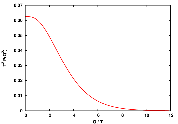
Figure 8: The distribution of $Q^{2}$ values between pairs of massless partons at temperature $T$ assuming respective Boltzmann distributions. It is not peaked, but its width scales with $T^{2}$.

Let us now consider a non-perturbative quantity, like the string tension, which is zero above $Q^{2}=\Lambda^{2}$ and around constant below this momentum scale. The ideal order parameter is given by a step function, $o=\Theta(\Lambda^{2}-Q^{2})$. The expectation value of such an order parameter at temperature $T$ is

$$\langle{o}\rangle=\int_{0}^{\Lambda^{2}}\limits\!d{Q^{2}}\,P(Q^{2})=\int_{0}^{\Lambda^{2}/T^{2}}\limits\!F(x)dx$$ (77)

by using the integration variable $x=Q^{2}/T^{2}$. This is the integrated distribution function of the thermal $Q^{2}$ distribution. By definition this approaches the value one from below, so as a function of $T$ (or $T^{2}$) it starts with the value $1$ and continuously decreases.

For high enough temperature, $T\gg\Lambda$, the distribution is nearly constant, so we can use (75) to conclude that

$$\langle{o}\rangle\approx\frac{c^{2}\Lambda^{2}}{T^{2}}.$$ (78)

For Boltzmann distribution $c=1/4$. This means that at any temperature there are non-perturbative (NP) effects to subleading order in $T^{2}$ (cf. the $1/16x^{2}$ curve on Fig.9).

Figure 9: The integrated distribution of $Q^{2}$ values from zero to $\Lambda^{2}$ as a function of $T/\Lambda$ in order to show the contribution of an NP order parameter. The dotted line is the high-temperature limit for the Boltzmann distribution.

In particular for the equation of state (EoS) of high-temperature matter, among others for the quark-gluon plasma, NP effects are present already at this level. Owing to the fact that the pressure be zero in the confining phase, one may consider that it is proportional to $1-\langle{o}\rangle$:

$$p=p_{SB}\left(1-\langle{o}\rangle\right).$$ (79)

Figure 10 plots the normalized pressure with this simple assumption and QCD lattice equation of state data from different groups. The cut-off parameter was taken as $\Lambda=6T_{c}=1$ GeV. The deviation from the Stefan-Boltzmann limit is non-perturbative, showing the subleading order at high temperature.

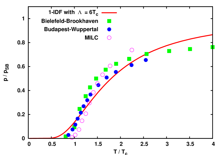
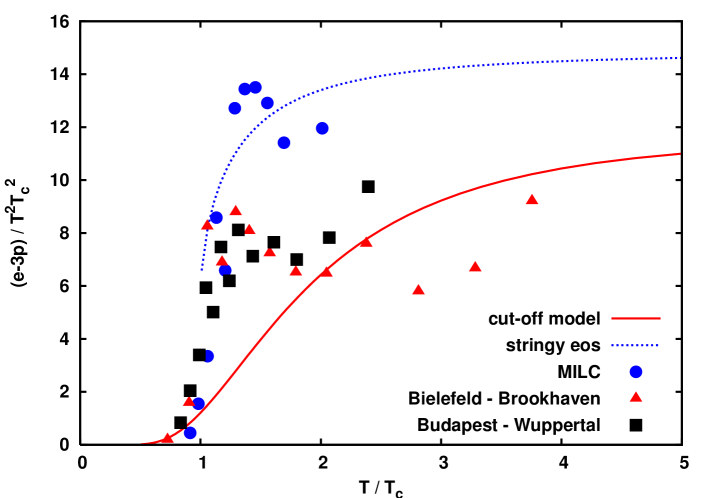
Figure 10: Normalized pressure as the expectation value of $1-\langle{o}\rangle$ assuming $\Lambda=6T_{c}\approx 1$ GeV and lattice results (top) and the scaled interaction measure (cf. eq.81) (bottom). The EoS curve for stringy matter is from Ref.STRINGY3 .

The interaction measure is also non-perturbative to leading order

$$e-3p=2c_{NP}\Lambda^{2}T^{2}+\ldots$$ (80)

Lattice gauge field theory calculations, especially SU(3) Yang-Mills, in fact show a rather constant value for the parameter

$$\Delta=\frac{e-3p}{T^{2}T_{c}^{2}},$$ (81)

(cf. Figure 10). The perturbative QCD predicts here effects going with $T^{2}\alpha(T)$, which has to be smaller than this. (The problem is that $\alpha(T)=\langle{\alpha(Q^{2})}\rangle$ also must contain NP effects, the one-loop inverse logarithm is not integrable with the $P(Q^{2})$ distribution.)

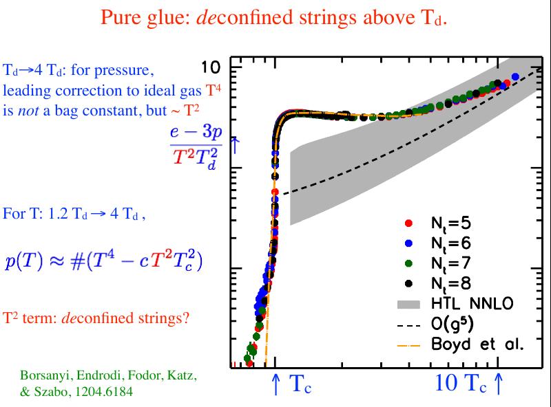
Figure 11: $T^{2}$-scaling of the interaction measure in pure glue lattice data. This is a slide from Rob Pisarski’s lecture on July 8th, 2016, Wigner RCP Theory Seminar, Budapest.

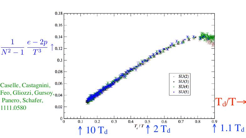
Figure 12: $T^{2}$-scaling for $2+1$ dimensional lattice data for different SU(N) gauge groups. This is a slide from Rob Pisarski’s lecture on July 8th, 2016, Wigner RCP Theory Seminar, Budapest.

Elementary thermodynamics of ideal gases including string-like objects, gives account to this subleading behavior. Here we briefly describe this mechanism based on the more detailed presentation in Ref.STRINGY3 . We denote the number density of colored sources by $c=\sum c_{i}n_{i}$ and assume that the temperature and number density dependent free energy density is given by

$$f\>=\>f_{{\rm id}}(n_{i},T)\,+\,\sigma\,\left\langle{\>\ell\>}\right\rangle\,c$$ (82)

with $\left\langle{\>\ell\>}\right\rangle=c^{-\gamma}$. For straight color tubes with constant cross sectional area in three dimensions one naturally assumes $\gamma=1/3$. In this way the total free energy density contains a term depending on the total color density as a fractional power:

$$f\>=\>f_{{\rm id}}(n_{i},T)\,+\,\sigma\,c^{1-\gamma}.$$ (83)

The chemical potentials, the pressure and energy density can be derived from this as follows

$$\mu_{i}\> = \>{\frac{\partial f}{\partial n_{i}}}\>=\>\mu_{i,{\rm id}}\,+\,(1-\gamma)\sigma c^{-\gamma}\,c_{i},$$

$$p\> = \>\sum\mu_{i}n_{i}-f\>=\>p_{{\rm id}}\,-\,\gamma\sigma c^{1-\gamma},$$

$$e\> = \>f-T{\frac{\partial f}{\partial T}}\>=\>e_{{\rm id}}\,+\,\sigma c^{1-\gamma}.$$ (84)

Utilizing these results the interaction measure becomes

$$\Delta\>=\>e-3p\>=\>e_{{\rm id}}-3p_{{\rm id}}+(1+3\gamma)\sigma\,c^{1-\gamma}.$$ (85)

The contribution by the ideal gas is zero for massless objects, for each massive degree of freedom it is proportional to $m^{2}$. For a QGP made of (nearly) massless quarks and gluons only the stringy contribution remains, in which all densities are proportional to $T^{3}$, as $n_{i}=\nu_{i}T^{3}$. In this case one obtains

$$\left.(e-3p)\right|_{m=0}\>=\>(1+3\gamma)\sigma\left(\sum c_{i}\nu_{i}\right)^{1-\gamma}\,T^{3(1-\gamma)}.$$ (86)

For straight objects $\gamma=1/3$, and this term is proportional to $T^{2}$, and the same follows for the non-ideal contribution to the total pressure, too:

$$p\>=\>\sigma_{SB}T^{4}-\frac{1}{3}\sigma\,\left(\sum c_{i}\nu_{i}\right)^{2/3}\,T^{2}.$$ (87)

A further remarkable property of this picture is that at the edge of mechanical stability, defined by vanishing total pressure, $p=0$, the energy density is given by

$$\left.e\right|_{p=0}\>=\>e_{{\rm id}}\,+\,p_{{\rm id}}/\gamma.$$ (88)

For massless constituents in the QGP $e_{{\rm id}}=3p_{{\rm id}}$, and $p_{{\rm id}}=T\sum n_{i}$, and we obtain the following energy per particle

$$\frac{E}{N}\>=\>\frac{e}{\sum n_{i}}\>=\>(3+1/\gamma)T\>=\>6T.$$ (89)

For a hadronization temperature of $167$ MeV, conjectured in earlier lattice calculations, this would be $E/N=1$ GeV; a value remarkably close to the result of phenomenological fits of hadronic ideal gas mixtures (the so called ”Statistical Model”) to heavy ion experiments at various bombarding energiesSTM1 ; STM2 ; STM3 ; STM4 ; STM5 . Since the hadronic matter has almost zero pressure compared to a QGP, the deconfinement phase crossover transition temperature is indeed close to the mechanical instability point defined by $p=0$.

Having a glimpse on Fig.12 one realizes that the nonperturbative leading correction to ideal pressure term is negative and scales with the Casimir of the charge in the $SU(N)$ gauge group, namely with $N^{2}-1$. Since strings pull, it is natural that they give a negative correction to the ideal pressure. Since they are mainly made of chromoelectric flux, it is natural that the effective string tension scales like $N^{2}-1$. However, for also resulting in ${\cal O}(T^{2})$ corrections, in $2+1$ dimensional lattices the elementary correction per color source must be like $f/c\sim\sigma\ln\left\langle{\>\ell\>}\right\rangle$. This hints towards a very different mechanism for the origin of such corrections in lower dimensional Yang-Mills systems.

Summarizing this subsection, we have shown on the basis of general arguments that non-perturbative effects, even those which cease at a sharp momentum cut-off, contribute to thermal expectation values at arbitrary high temperatures. Based on the thermal distribution of $Q^{2}$ values it was demonstrated that this contribution is of the relative order of $\Lambda^{2}/T^{2}$ to any thermally averaged quantity. A physical picture of such non-perturbative corrections to the ideal gas equation of state is offered by an elementary study of the thermodynamics of straight strings with a naturally density-dependent average length.

4.5 Shear viscosity bounds

Accelerator experiments suggest that the matter formed in heavy ion collisions is a very good fluid close to be a perfect one Shuryak:2003xe ; Teaney:2003kp , which means that the characteristic dimensionless $\eta/s$ ratio ($\eta$ being the shear viscosity, $s$ the entropy density) is very small. The quantity $\eta/s$, apart from the fact that it appears directly in hydrodynamical formulas like the sound attenuation length Landau , can be interpreted as a fluidity measure of an ultra-relativistic gas that characterizes the viscosity on its own scale Liao:2010nv .

The experimental tool to access this quantity is measuring the flow anisotropy, in particular its second angular moment, $v_{2}$. The desired parameters of the corresponding fluid model can be obtained by fitting the model predictions to the experimental curves Romatschke:2007mq ; Dusling:2007gi . The result of these studies is that the observed $\frac{\eta}{s}\sim\frac{1}{4\pi}$ with a coefficient of order one. The value $\frac{1}{4\pi}$ has a specific significance, since, at is it used to say, it is the “theoretical lower bound”.

But, as opposed to the folklore, the status of $1/4\pi$ being a theoretical lower bound for the $\eta/s$ ratio, is far from being proven. We try to review in this section what are the assumptions and approximations behind this conjecture.

The idea that $\eta/s$ can have a lower bound, was first suggested in Danielewicz:1984ww . The authors realized that in the kinetic approach $\eta/s\sim E\tau$ where $E$ is the quasiparticle energy and $\tau$ is its lifetime. For a quasiparticle $E>\Delta E$ where $\Delta E$ is the width of the quasiparticle peak, therefore, using uncertainty principle $\eta/s\sim E\tau>\Delta E\tau\gtrsim\hbar$, meaning that $\eta/s$ has a lower bound. This elegant way of thought, however, cannot be considered as a proof of the lower bound, since it uses the kinetic, quasiparticle approach which is not really suitable to describe the small viscosity regime. The point is that kinetic theory estimates the shear viscosity to be $\eta\sim 1/\sigma$ where $\sigma$ is a cross section. In weakly coupled theories $\sigma\sim g^{4}$ where $g$ is the coupling constant. Since $g$ must be small in order the kinetic, Boltzmann-equation approach be applicable, only the large viscosity regime is accessible in this way. In this range of applicability several studies in the literature computed the shear viscosity using the Boltzmann-equation or quasiparticle approach Peshier ; Dobado:2009ek ; Marty:2013ita ; Kadam:2014cua ; Bluhm:2010qf ; Hidaka:2009ma . But, when the theory is more and more strongly coupled, higher order processes become dominant, too Xu:2007ns ; Xu:2007jv , and the simplest kinetic argumentation looses its validity.

One can think that perturbation theory is also can be used to calculate the $\eta/s$ ratio. The entropy density is defined through the thermodynamics from free energy, the shear viscosity by the Kubo formula

$$\eta=\lim\limits_{\omega\to 0}\frac{\left\langle[T_{12}(\omega,{\bm{k}}=0),T_{12}(x=0)]\right\rangle}{\omega}.$$ (90)

But with the perturbative approach there are several problems. The first one is that in realistic applications, for example for QCD near the critical regime of the crossover perturbation theory is not really applicable. At somewhat higher temperatures the perturbation theory still needs heavy machinery including resummations to reliably predict the thermodynamical quantities like pressure or entropy density, but after some efforts one can give a relatively good description Andersen:2015eoa . But the shear viscosity is a quantity that is much harder to access. The fundamental problem is that perturbation theory can compute corrections to a quantity calculated in the free theory. But the shear viscosity is infinite in a free gas. Therefore we should compute corrections to infinity which is a hard task. In a strict diagrammatic approach one has to re-sum ladder diagrams Jeon:1994if ; Carrington:2002bv . One can use 2PI resummation to perform the task Aarts:2004sd , or, concentrating only to the most important pinch singular contributions, quantum Boltzmann-equations Arnold:2000dr ; Arnold:2002zm ; Arnold:2003zc ; Jakovac:2001kj . One can also apply renormalization group techniques to approach the shear viscosity Haas:2013hpa But even after the most thorough job one can expect a “small” correction to infinity that means large numerical values: one typically gets $\eta\sim 1/(g^{4}\log g)$ as the leading order estimate. For small viscosities, just like in the kinetic approach, we would need large coupling, and so perturbation theory is not applicable there.

An alternative approach to calculate the shear viscosity could be the lattice Monte Carlo technique. There have been in fact attempts to extract this information from lattice, calculating the energy-momentum tensor correlation function Karsch:1986cq ; Meyer:2007dy . The obtained results have been in the $\eta/s\sim 0.1-0.2$ regime. Unfortunately the measurements cannot be performed without strong assumptions. The reason is that hydrodynamics is an effective description of the matter only in so large timescales that is hard to access from a Euclidean lattice. Therefore the present MC simulations have very small sensitivity to the desired transport regime Datta:2008dq . We remark that in classical theories one can also compute the shear viscosity Homor:2015qza . Here one is not restricted by the Euclidean formalism, but the quantum interpretation is much more difficult.

Since small viscosity involves large couplings, therefore methods that use the inverse coupling as expansion parameters are of great importance. Unfortunately these dual partners are rarely known. Therefore the conjectured AdS/CFT duality Maldacena:1997re has a big relevance, even though here the weakly coupled theory is a conformal field theory, and so its symmetries are not the same as the symmetries of QCD. Nevertheless one can calculate the $\eta/s$ ratio in the infinitely strongly coupled (the t’Hooft coupling $\lambda=g^{2}N_{c}$ is infinite) ${\cal N}=4$ supersymmetric Yang-Mills theory with this method Kovtun:2004de resulted in $\eta/s=1/{4\pi}$. The significance of this result is raised by the fact that the infinitely coupled theory is expected to have the smallest shear viscosity; in fact, in this model the $1/\lambda$ corrections are all positive Myers:2008yi . The KSS result, together with the conjecture of the lower bound based on kinetic approach was then advertised that “the lower bound for the $\eta/s$ ratio is $1/(4\pi)$”.

But, as we see, the two pivots of the argumentation are coming from the quasiparticle and the conformal field theory limits, and so these are not as general as it is usually thought. In fact, soon after the announcement of the “lower bound” there appeared constructions that violate, or at least challenge the $1/(4\pi)$ value.

In the framework of non-relativistic theories one can construct such theories Cohen:2007qr ; Cherman:2007fj ; Son:2007xw ; for example theories where with the growing number of field components the shear viscosity remains constant, but the entropy density grows with the number of the components. It is also seems valid that when we start to deviate from the quasiparticle approximation, for example with the inclusion of the continuum besides the quasiparticle peak, the shear viscosity starts to decrease NoronhaHostler:2008ju ; Jakovac:2009xn ; Horvath:2015gqd . In fact, in very general grounds one can argue for a lower bound not for $\eta/s$, but $\eta T^{3}/s^{2}$ Jakovac:2009xn ; Horvath:2015gqd .

From the Ads/CFT side, there are also doubts about the universality of the $1/(4\pi)$ bound. Model studies of gravity models, where besides the leading order AdS action there are corrections (higher order terms in curvature, other fields like dilaton) lead to the conclusion that in these models the $\eta/s$ ratio can ge below $1/(4\pi)$ Kats:2007mq ; Buchel:2008vz ; Cai:2009zv ; Feng:2015oea . It is not clear if in a general consistent gravity model there exists at all a lower bound.

From experimental side it seems that the $\eta/s$ ratio of the strongly interacting plasma is ${\cal O}(1-2)/(4\pi)$ Romatschke:2007mq ; Drescher:2007cd ; Lacey:2013eia . Comparing with the $\eta/s$ values of other matters like water or even superfluid ⁴He, the $\eta/s$ value really seems very low Lacey:2006bc , but if we use a fluidity measure better suited for not ultra-relativistic matter, then QCD seems to be not extraordinary Liao:2010nv .

So, summarizing the content of this section, although in quasiparticle systems and some conformal theories we really expect to have a lower bound for the shear viscosity, but in a strongly interacting matter like QCD there is no well-established proof for that. It is also true, that the numerical value of $1/(4\pi)$ is so small, that it is not easy to provide such experimental setup where we could violate this bound. But, since this bound is not a constant of nature, it can happen that in some future collider experiments it will still be violated.

4.6 Rather field or rather particle?

The particle-wave duality appears in an interesting aspect in the heavy ion collisions. The classical picture of a particle is a point-like object traveling on a world-line in the spacetime; if the particle is free of interaction, the world-line is a straight line (or geodesic line). On the other hand the free quantum particle has infinite extension in space as a plane wave.

Interacting particles or waves penetrating and trespassing a medium get distorted. The distortion effect depends on the nature of the interaction, its localization and strength. Typically particle-like interactions are extremely localized, not only in space, but also in time. The straight world-line receives kicks once in a while. An extended medium on the other hand acts for long and makes the particle world-line smoothly curved. The same typing for extended waves includes changes in the dispersion relation by phase shifts in the former case and an overall change in the latter case. Static and large media, in particular, modify the free particle dispersion relations (propagators) by inducing a self-energy part, which re-scales the effective mass and adds a quasi-particle width. A continuum part in a spectral function, however, is a sign for creating and annihilating particles during the interaction between the quantum objects and the medium.

Traditional high-temperature field theory considers the environment as given, in most cases keeping a sharp value of the temperature. This so called heat bath is assumed to be god given and very few thoughts are dedicated to the problem: where does this temperature comes from? What mechanism keeps its value so constant? And how should we describe the QGP if none?

In principle all thermal effects are results of the same interaction. It is therefore legitim to seek for approaches which do not assume a temperature, but calculate it. Or at least investigate the effects due to un-sharp values of it – a step forward – testing some simple distributions. This so called superstatistical approachTSALLISorig ; TSALLISBOOK ; Beck1 ; BeckCohen ; Cohen ; Beck2 ; ABC is based on a particular distribution of $\beta$ values in the thermal weight, $\exp{(-\beta H)}$. The simplest such distribution, having a width of $\beta$-values and allowing only non-negative ones, is an Euler–Gamma distribution. This converts the Boltzmann–Gibbs weight in a Tsallis–Pareto form:

$$\int_{0}^{\infty}\limits\,\,\mathrm{e}^{-\beta H}\,\,\frac{(\beta nT)^{n-1}}{\Gamma(n+1)}\,\,\mathrm{e}^{-\beta nT}\,\,nTd\beta\>=\>\left(1+\frac{H}{nT}\right)^{-n},$$ (91)

often experienced in particle spectra measured in high-energy collisions. Here $\left\langle{\>\beta\>}\right\rangle=1/T$ and $\Delta\beta/\left\langle{\>\beta\>}\right\rangle=1/\sqrt{n}$. In the $n\to\infty$ limit the distribution of $\beta$ values narrows to a Dirac delta, and the above statistical weight converts to the well-known Boltzmann factor. Candidates for physical mechanisms therefore, which would explain the occurrence of the temperature, $T$, in a dynamical system, should also explain whether or not the width $\Delta\beta$ is small enough under the circumstances given.

A thermodynamical interpretation of the parameters $T$ and $n$ can be given starting from Einstein’s idea relating the statistically evenly occupied phase space volume to the notion of entropyBiroENTROPY ; BiroPHYSICA ,

$$\Omega(E)\>=\>\,\mathrm{e}^{S(E)}\,.$$ (92)

Picking up a subsystem with energy $H$ out of $E$ has then the probability

$$P(H)\>=\>\frac{\Omega(H)\,\Omega(E-H)}{\Omega(E)},$$ (93)

assuming no correlation other than induced by fixing the total energy to $E$. In this microcanonical view the environmental factor,

$$\rho(H)\>=\>\left\langle{\>\frac{\Omega(E-H)}{\Omega(E)}\>}\right\rangle,$$ (94)

models the statistical operator. Based on the conjectured connection to the thermodynamical entropy one finally deals with

$$\rho(H)\>=\>\left\langle{\>\,\mathrm{e}^{S(E-H)-S(E)}\,\>}\right\rangle.$$ (95)

In the expansion $H\ll E$ up to quadratic terms one obtains

$$\rho(H)\>=\>1\,-\,H\left\langle{\>S^{\prime}(E)\>}\right\rangle\,+\,\frac{1}{2}H^{2}\,\left\langle{\>S^{\prime\prime}(E)+S^{\prime}(E)^{2}\>}\right\rangle\,+\,\ldots$$ (96)

Comparing this result with eq.(91) one interprets the parameters as

$$\frac{1}{T}\>=\>\left\langle{\>S^{\prime}(E)\>}\right\rangle\qquad\mathrm{and}\qquad T^{2}\Delta\beta^{2}\>=\>\frac{1}{C}+\frac{1}{n},$$ (97)

with $C=dE/dT$ being the total heat capacity of the system. In the infinite reservoir (thermodynamical) limit, $C\to\infty$, one gets back the width of the Euler–Gamma distribution. On the other hand, for $n\to\infty$, considering a sharp $\beta$ value, one obtains the textbook result $T^{2}\Delta\beta^{2}=1/C$ for the variance. Indeed near to the maximum the Euler–Gamma distribution, as many other, is well approximated by a Gaussian. However, the Gaussian assumption cannot be extended to negative $\beta$ values, therefore the Euler–Gamma assumption is superior.

In interacting, ”real” systems the natural dynamics itself must determine the actual distribution of $\beta$ values. For any finite sized system, a width of this distribution is compulsory. The task of understanding the emergence of temperature and other thermal effects, and calculating the actual values of $T$ and $C$, and perhaps $n$ in existing physical systems, sharpens even more in quantum (field) theory. If $\beta$, or for that matter any function of it, is associated to an operator in the quantum description, then its width cannot be narrowed down to zero in practice. (Only theoretically, on the cost of having infinite width for other, non-commuting operators.) Here the question to be answered is, how to describe a statistical operator part during the quantum evolution, which – under certain approximations to the physical reality – behaves like factorizing to a Boltzmann-Gibbs, or similar, and a unitary factor.

For this purpose considering quantum states with finite width can be of help. Contrary to point-particles (zero width in location, infinite width in momentum) and to plane-waves (infinite width in location, zero width in momentum) more general states, in particular coherent states look more realistic. In the rest of this section we give a short overview of properties of coherent states and show a possible way of an unusual interpretation of being thermal.

4.6.1 State labels

We consider generalized coherent states defined by

$$\left|\,{z}\,\right>=\sum_{n=0}^{\infty}\limits\sqrt{p_{n}(t)}\,e^{in\Theta}\,\left|\,{n}\,\right>$$ (98)

with $z=\sqrt{t}e^{i\Theta}$. Such constructions in quantum optics are called ”nonlinear coherent states”. This state overlaps with the $n$-quantum state, the overlap probability being

$$\left|\left<\,{n}\middle|{z}\,\right>\right|^{2}\>=\>p_{n}(t)\geq 0.$$ (99)

From the normalization of the coherent state, $\left|\,{z}\,\right>$, a normalization of the factor $p_{n}(t)$ follows:

$$\left<\,{z}\middle|{z}\,\right>\>=\>\sum_{n,m}\limits\left<\,{m}\,\right|\sqrt{p_{m}p_{n}}\,e^{i(n-m)\Theta}\left|\,{n}\,\right>\>=\>\sum_{n}p_{n}(t)=1.$$ (100)

The expectation value of any function of the number operator, $\hat{n}=a^{{\dagger}}a$, is given by

$$\left<\,{z}\,\right|\varphi(\hat{n})\left|\,{z}\,\right>\>=\>\sum_{n}\varphi(n)\,p_{n}(t).$$ (101)

This construction ensures that $p_{n}(t)$ is a probability distribution in ${n}$.

We also construct a complete set based on coherent states as follows:

$$\int\!\!\frac{d^{2}z}{\pi}\left|\,{z}\,\right>\left<\,{z}\,\right|\,=\,\int_{0}^{\infty}\limits\!\!dt\int_{0}^{2\pi}\limits\!\frac{d\Theta}{2\pi}\sum_{n,m}\limits\sqrt{p_{n}p_{m}}e^{i(n-m)\Theta}\left|\,{m}\,\right>\left<\,{n}\,\right|.$$ (102)

Here, after integrating over $\Theta$ one obtains a Kronecker $\delta_{nm}$ under the double sum and ends up with a single sum:

$$1\>=\>\int_{0}^{\infty}\limits\!\!dt\,\sum_{n}p_{n}(t)\left|\,{n}\,\right>\left<\,{n}\,\right|\>=\>\sum_{n}\left|\,{n}\,\right>\left<\,{n}\,\right|.$$ (103)

A sufficient condition for completeness is $\int_{0}^{\infty}\limits\!\!dt\,p_{n}(t)\>=\>1$, wishing a complete set for all possible Fock spaces based on $\left|\,{n}\,\right>$, it is also necessary. This makes $p_{n}(t)$ to a probability distribution function of $t$ as well. One may consider the distribution in the number of quanta $n$ as primary statistics, while in the coherent state parameter $t=|z|^{2}$ as superstatistics.

4.6.2 Operator eigenstate

While the most known coherent states show a Poisson statistics in $n$, and are eigenstates of the annihilation operator, $a$, the generalized versions are eigenstates to a more complex operator. To construct this operator is related to the problem of regularizing the phase operator in quantum optics PHASEOP1 ; PHASEOP2 ; PHASEOP3 ; PHASEOP4 .

We request that $\left|\,{z}\,\right>$, defined as in eq.(98), is an eigenstate with eigenvalue $z$ to the following operator:

$$F\left|\,{z}\,\right>\>=\>ag(\hat{n})\left|\,{z}\,\right>\>=\>z\,\left|\,{z}\,\right>.$$ (104)

Here $a$ is an annihilating ($a^{{\dagger}}$ is a creating) operator, and $\hat{n}=a^{{\dagger}}a$ is the number operator. $g(\hat{n})$ is a yet unspecified function of the number operator.

The action of this operator $F$ on the general coherent state causes

$$F\left|\,{z}\,\right>\>=\>\sum_{n=1}^{\infty}\limits g(n)\sqrt{np_{n}}\,e^{in\Theta}\left|\,{n-1}\,\right>,$$ (105)

that can be re-indexed to

$$F\left|\,{z}\,\right>\>=\>\sum_{n=0}^{\infty}\limits g(n+1)\sqrt{(n+1)p_{n+1}}\,e^{i(n+1)\Theta}\left|\,{n}\,\right>.$$ (106)

One can derive a recursion law by comparing this result with

$$z\,\left|\,{z}\,\right>\>=\>\sqrt{t}\,e^{i\Theta}\sum_{n=0}^{\infty}\limits\sqrt{p_{n}}\,e^{in\Theta}\left|\,{n}\,\right>.$$ (107)

In conclusion the following relation has to be satisfied:

$$p_{n}(t)\>=\>\frac{t}{ng(n)^{2}}\,p_{n-1}(t).$$ (108)

This specifies to a known quantum number distribution, $p_{n}(t)$, the necessary function $g(n)$, or serves as a recursion rule for a given $g(n)$, fixing the operator $F$, to obtain the distribution $p_{n}(t)$. The recursion is solved by

$$p_{n}(t)\>=\>p_{0}(t)\,\frac{t^{n}}{n!}\>{\prod_{j=1}^{n}\limits g(j)^{-2}}.$$ (109)

Finally $p_{0}(t)$ can be obtained from the normalization condition. At the end of this reconstruction also the completeness constraint, $\int_{0}^{\infty}\limits\!\!dt\,p_{n}(t)\>=\>1$, has to be checked.

4.6.3 Glauber and Negative Binomial states

The most known, traditional coherent state is defined by $\bm{g(n)=1}$. This results in a Poisson distribution in $n$ and in an Euler-Gamma distribution in $t$:

$$p_{n}(t)\>=\>\frac{t^{n}}{n!}\,e^{-t}.$$ (110)

In this case $\left|\,{z}\,\right>$ is an eigenstate to the $F=a$ annihilation operator.

The negative binomial coherent state is based on the negative binomial distribution (NBD),

$$p_{n}(t)\>=\>\binom{n+k}{n}\,(t/k)^{n}\,(1+t/k)^{-n-k-1}.$$ (111)

It is a normalized NBD in $n$, and at the same time is an Euler-Beta distribution in $t$. From the recursion eq.(108) one obtains the necessary $g(n)$ function for modifying the operator $a$ to $F=ag(\hat{n})$:

$$g(n)^{2}\>=\>\frac{t}{n}\,\frac{p_{n-1}}{p_{n}}\>=\>\frac{k+t}{k+n},$$ (112)

so this NB coherent state satisfies

$$a\sqrt{\frac{k+|z|^{2}}{k+a^{{\dagger}}a}}\,\left|\,{z}\,\right>\>=\>z\,\left|\,{z}\,\right>.$$ (113)

One realizes a one-dimensional boost property beyond such NB states when introducing the rapidity-like notation: $t/k=\sinh^{2}\zeta$. Using this notation the distribution and the Fock-representation of such a state are rewritten as

$$p_{n}(t)=\binom{k+n}{n}\,\sinh^{2n}\zeta\,\cosh^{-2n-2k-2}\zeta,$$

$$\left|\,{z}\,\right>=\sum_{{n}=0}^{\infty}\limits\!\sqrt{\binom{k+n}{n}}\,\frac{\left(e^{i\Theta}\,\tanh\zeta\right)^{n}}{\cosh^{k+1}\zeta}\left|\,{n}\,\right>.$$ (114)

Using the velocity variable $v=\tanh\zeta$, the corresponding Lorentz factor is given by $\gamma=\cosh\zeta$ and the overlap probability between two NB coherent states becomes

$$\left|\left<\,{z_{1}}\middle|{z_{2}}\,\right>\right|^{2}\>=\>\left[1+\gamma_{1}^{2}\gamma_{2}^{2}\left|v_{1}e^{i\Theta_{1}}-v_{2}e^{i\Theta_{2}}\right|^{2}\right]^{-k-1}.$$ (115)

This result reminds us to a Tsallis–Pareto distribution with the energy variable replaced by a relative velocity squared in a 2+1 dimensional vector notation. The possibility of using such a notation is related to the $su(1,1)$ algebra structure of operators forming an NB coherent state, an interesting connection which shall be discussed below.

For this purpose it is enlightening to express the overlap between NB coherent states in terms of the complex numbers $z_{1}$ and $z_{2}$. We introduce the following vector,

$$\vec{K}=\gamma_{1}\gamma_{2}\left(\vec{v}_{1}-\vec{v}_{2}\right)\>=\>\frac{1}{\sqrt{k}}\,\left(\gamma_{2}z_{1}-\gamma_{1}z_{2}\right).$$ (116)

The NB state overlap written this way converges to the known overlap between Glauber coherent states for large $k\to\infty$:

$$\left|\left<\,{z_{1}}\middle|{z_{2}}\,\right>\right|^{2}\>=\>\left[1+\frac{1}{k}\left|\gamma_{2}z_{1}-\gamma_{1}z_{2}\right|^{2}\right]^{-k-1}\to e^{-|z_{1}-z_{2}|^{2}}.$$ (117)

with $\gamma_{i}=\sqrt{1+|z_{i}|^{2}/k}\to 1$. It is an interesting question whether we can connect some physical property of particle-like objects to this quantity. Interpreting the $v_{i}$-s as magnitudes of velocities and obtaining the corresponding Lorentz factors from the energy to mass ratio of pointlike massive objects one would consider

$$\vec{K}=\frac{1}{m_{1}m_{2}}\left(E_{2}\vec{P}_{1}-E_{1}\vec{P_{2}}\right).$$ (118)

In this interpretation the overlap between two NB states decays asymptotically as a power-law of the relative velocity of relativistic massive particles moving on a plane.

It is useful to extend the notation of NB states with the index $k$, referring to the $k$ parameter in the underlying NBD distribution. From now on we use the following notation

$$\left|\,{z_{k},k}\,\right>\>=\>\sum_{n=0}^{\infty}\limits\sqrt{p_{n}(k)}e^{in\Theta}\left|\,{n}\,\right>$$ (119)

with $z_{k}=\sqrt{kf}\,e^{i\Theta}$ for the NB states and

$$p_{n}(k)\>=\>\binom{k+n}{n}\,f^{n}\,(1+f)^{-n-k-1}$$ (120)

for the NBD distribution. This distribution provides an average number of $\left\langle{\>n\>}\right\rangle=(k+1)f$.

We are primarily interested in the effect of annihilating a quantum from an NB state. The annihilating ladder operator acts as

$$a\left|\,{z_{k},k}\,\right>\>=\>\sum_{n=1}^{\infty}\limits\sqrt{p_{n}}e^{in\Theta}\,\sqrt{n}\left|\,{n-1}\,\right>$$ (121)

what can be re-indexed into

$$a\left|\,{z_{k},k}\,\right>\>=\>\sum_{n=0}^{\infty}\limits\sqrt{(n+1)p_{n+1}}\,e^{i\Theta}\,e^{in\Theta}\left|\,{n}\,\right>.$$ (122)

Consider now that

$$(n+1)p_{n+1}(k)\>=\>(n+1)\binom{k+n+1}{n+1}f^{n+1}(1+f)^{-(n+1)-k-1}$$ (123)

can be expressed as

$$(n+1)p_{n+1}(k)\>=\>f({k+1})\,\binom{k+1+n}{k+1}f^{n}(1+f)^{-n-(k+1)-1}.$$ (124)

Here we recognize $z_{k+1}=\sqrt{f(k+1)}e^{i\Theta}$ as a factor and arrive at the elegant result

$$a\,\left|\,{z_{k},k}\,\right>\>=\>z_{k+1}\left|\,{z_{k+1},k+1}\,\right>.$$ (125)

In the $k\to\infty$ limit again the familiar Glauber coherent state emerges, as an eigenstate of the annihilation operator, $a$. On the other hand for an NB state, the annihilation of a primary quantum can be represented by an upgrade of the parameter $k$ by one, times the corresponding complex eigenvalue, $z_{k+1}$. This helps us to answer the question of to what operator is an NB state an eigenstate. We compare the above result with the action of another operator

$$\sqrt{\hat{n}+k+1}\,\left|\,{z_{k},k}\,\right>\>=\>\sqrt{(k+1)(1+f)}\,\left|\,{z_{k+1},k+1}\,\right>,$$ (126)

based on the relation

$$(k+1+n)\,\binom{k+n}{k}\>=\>(k+1)\,\binom{k+1+n}{k+1}.$$ (127)

This helps to recognize the following NB eigenvalue equation:

$$\left(\sqrt{f}\,(\hat{n}+k+1)-\sqrt{1+f}\,e^{-i\Theta}\,\sqrt{\hat{n}+k+1}\>a\right)\,\left|\,{z_{k},k}\,\right>\>=\>0.$$ (128)

Based on this it is now easy to work out the corresponding NB algebra. In the previous eigenvalue equation (128) the following operator occurs:

$$K_{-}\>=\>\sqrt{\hat{n}+k+1}\,a,\qquad K_{+}\>=\>K_{-}^{{\dagger}}\>=\>a^{{\dagger}}\,\sqrt{\hat{n}+k+1}.$$ (129)

Their commutator,

$$\left[K_{-},K_{+}\right]\>=\>(\hat{n}+1)(\hat{n}+k+1)-\hat{n}(\hat{n}+k)\>=\>2\hat{n}+k+1\>=\>2K_{0}$$ (130)

defines $K_{0}\>=\>\hat{n}+(k+1)/2$ as a linear expression using $\hat{n}$. With $\alpha=\sqrt{(1+f)/f}\,e^{-i\Theta}$ we arrive at

$$\left(\alpha\,K_{-}-\,K_{0}\right)\,\left|\,{z,k}\,\right>\>=\>\frac{k+1}{2}\cdot\left|\,{z,k}\,\right>.$$ (131)

The commutators among the $K$-operators form an SU(1,1) algebra:

$$\left[K_{0},K_{+}\right]\> = \>K_{+}$$

$$\left[K_{0},K_{-}\right]\> = \>-K_{-}$$

$$\left[K_{-},K_{+}\right]\> = \>2K_{0}$$ (132)

The Casimir operator is given as: $Q=K_{0}^{2}-K_{0}-K_{+}K_{-}.$

4.6.4 Creation of an NB state from Fock vacuum

Another important question is how to create an NB state from the vacuum. For the ordinary coherent state a unitary operator, also called Weyl operator, does the job. For a more general analysis we consider again general functions of the number operator, $\hat{n}$, mixed with annihilation and creation operators. This describes a coupling to a field with field-energy dependent coefficients.

The known operator identity,

$$e^{A+B}\>=\>e^{-\lambda/2}\,e^{A}\,e^{B}\qquad{\mathrm{with}}\qquad[A,B]\>=\>\lambda,$$ (133)

if $[A,\lambda]=0$ and $[B,\lambda]=0$, helps us to obtain the necessary form for $\left|\,{z_{k},k}\,\right>=U\left|\,{0}\,\right>$. We choose  $A=\alpha\,zf(\hat{n})\,a^{{\dagger}}$  and  $B=-\beta\,z^{*}a\,/f(\hat{n})$. Please note that $B\neq-A^{{\dagger}}$. The commutator,

$$[A,B]=|z|^{2}\alpha\beta\,\left(a\frac{1}{f(\hat{n})}f(\hat{n})a^{{\dagger}}-f(\hat{n})a^{{\dagger}}a\frac{1}{f(\hat{n})}\right)$$ (134)

leads to $\lambda=|z|^{2}\alpha\beta$. We seek our evolution operator from the Fock vacuum to an NB state in the form

$$U\>=\>e^{\Phi/2+A+B}\>=\>e^{(\Phi-\lambda)/2}\,e^{A}\,e^{B}.$$ (135)

Here $e^{B}\left|\,{0}\,\right>=\left|\,{0}\,\right>$ due to $B\left|\,{0}\,\right>=0$, since $B$ in the exponent is proportional to the annihilation operator. Expanding the exponential one obtains

$$U\left|\,{0}\,\right>\>=\>e^{(\Phi-\alpha\beta\,|z|^{2})/2}\,\sum_{{n}=0}^{\infty}\limits\!\frac{\alpha^{n}z^{n}}{n!}\left(f(\hat{n})a^{{\dagger}}\right)^{n}\,\left|\,{0}\,\right>.$$ (136)

Since we have

$$\left(f(\hat{n})a^{{\dagger}}\right)^{n}\,\left|\,{0}\,\right>\>=\>f(n)\cdot\ldots\cdot f(1)\,\sqrt{n!}\,\left|\,{n}\,\right>,$$ (137)

the form

$$U\left|\,{0}\,\right>\>=\>\sum_{{n}=0}^{\infty}\limits\!\sqrt{u_{n}}\,e^{in\Theta}\left|\,{n}\,\right>,$$ (138)

with $z=\sqrt{t}\,e^{i\Theta}$, is achieved when using $f(\hat{n})=\xi\,\sqrt{\hat{n}+k}$:

$$u_{n}=e^{\Phi-\alpha\beta\,t}\,\left(\alpha^{2}\xi^{2}t\right)^{n}\,\binom{n+k}{n}.$$ (139)

In order to satisfy normalization of the resulting NB state, $||U\left|\,{0}\,\right>||^{2}=1$, one needs

$$\sum_{{n}=0}^{\infty}\limits\!u_{n}\>=\>e^{\Phi-\alpha\beta t}\,\left(1-\alpha^{2}\xi^{2}t\right)^{-(k+1)}\>=\>1.$$ (140)

From this we express

$$\alpha^{2}\xi^{2}t=1-e^{\frac{1}{k+1}(\Phi-\alpha\beta t)}\>=\>1-w,$$ (141)

and gain the following negative binomial distribution:

$$u_{n}\>=\>\binom{n+k}{n}\,w^{k+1}\,(1-w)^{n}.$$ (142)

For the superstatistics normalization, we utilize the Euler Beta integral

$$\int_{0}^{\infty}\limits\!dt\,u_{n}(t)\>=\>\binom{k+n}{n}\,\int_{0}^{\infty}\limits\!dt\,w^{k+1}(1-w)^{n},$$ (143)

which after changing the integration variable from $t$ to $w$ should become unity:

$$\int_{0}^{\infty}\limits\!dt\,u_{n}(t)\>=\>\binom{k+n}{n}\,k\,\int_{0}^{1}\limits dw\,w^{k-1}(1-w)^{n}\>=\>1.$$ (144)

This condition is satisfied if

$$dt=-k\frac{dw}{w^{2}},\qquad\longrightarrow\qquad t\>=\>k\,\left(\frac{1}{w}-1\right),$$ (145)

or – expressing $w(t)$ – the superstatistics is normalized if

$$w\>=\>\frac{1}{1+t/k}\>=\>\frac{k}{t+k}.$$ (146)

This requirement identifies $\Phi$ as being

$$\Phi\>=\>\alpha\beta\,t-(k+1)\ln\left(1+t/k\right)$$ (147)

After these manipulations only $\alpha,\beta$ and $\xi$ remain undetermined. A purposeful choice is $\alpha=\beta=1/\sqrt{t}=1/|z|$ with $\xi=1/\sqrt{t+k}$. The natural logarithm of the evolution operator becomes in this case

$$\ln U\> = \>-\frac{k+1}{2}\ln\left(1+t/k\right)+\frac{1}{2}$$ (148)

$$-\,e^{-i\Theta}\,a\,\sqrt{\frac{t+k}{\hat{n}+k}}+\,e^{i\Theta}\sqrt{\frac{\hat{n}+k}{t+k}}\,a^{{\dagger}}.$$

This is neither Hermitean nor anti-Hermitean, therefore can only be interpreted as

$$\ln U\>=\>-\frac{1}{2}\,\beta H_{0}+\frac{i}{\hbar}\tau H_{1}.$$ (149)

With this definition one has a statistical operator of

$$\rho\>=\>U^{{\dagger}}U\>=\>e^{-\beta H_{0}}.$$ (150)

This underlines the necessity of thinking in complex time paths or equivalently assuming an environmental factor, which is not unitary. The anti-Hermitean part of $\ln U$ gives a guess for the evolution Hamiltonian

$$\frac{i}{\hbar}\tau H_{1}\>=\>\,\mathrm{e}^{i\Theta}\,f_{+}(\hat{n})a^{{\dagger}}-\,\mathrm{e}^{-i\Theta}\,af_{+}(\hat{n}),$$ (151)

while the Hermitean part for the statistical factor

$$-\frac{1}{2}\beta H_{0}\>=\>R_{k}\,+\,\,\mathrm{e}^{i\Theta}\,f_{-}(\hat{n})a^{{\dagger}}+\,\mathrm{e}^{-i\Theta}\,af_{-}(\hat{n}).$$ (152)

Here

$$f_{\pm}\> = \>\frac{1}{2}\left(\sqrt{\frac{\hat{n}+k}{t+k}}\pm\sqrt{\frac{t+k}{\hat{n}+k}}\right),$$

$$R_{k}\> = \>\frac{1}{2}-\frac{k+1}{2}\ln(1+t/k).$$ (153)

Please note that in this case the statistical environmental operator contains a factor in the Tsallis–Pareto form:

$$\rho\>\propto\>\left(1+\frac{t}{k}\right)^{-k-1},$$ (154)

with $t=|z|^{2}$ interpretable as the average number of quanta in an NB state.

4.7 Physical sources of NB states

Various physical mechanisms may lead to an NBD in particle numbers produced in high energy collisions. The NB coherent state, reviewed above, is just one of them; more closely we did not specify the Hamiltonian which produces such a state. Typically, as described in eqs.(151) and (152), a linear field coupling of the particle modes, as described by the phase factors $\,\mathrm{e}^{\pm i\Theta}\,$ and the annihilation and creation operator, are necessary for the desired result. However, other than for the classical Glauber coherent state, the coupling (or equivalently the amplitude of the external field creating the particles) does depend on the number of particles to be produced. In particular for the NB coherent state this dependence is algebraic, involving the square root function – as specified in eq.(153). This effect is typically a multiparticle effect, the mathematical expression involves infinitely many quanta for the same mode.

There are further hints and speculations about the origin of negative binomial particle distributions. A simple phase space cell statistics, ”throwing” stones of quanta into phase space cells repeatedly in unrestricted number – as bosons behave – predicts a combinatoric factor in the probability to find exactly $n$ particles in $k$ cells. The Pólya distribution extends this picture to the same probability, when the investigated system of $n$ and $k$ is a part of a bigger system consisting of $N$ particles altogether in $K$ total number of phase space cells:

$$P_{n}\>=\>\frac{\binom{k+n}{n}\,\binom{K-k+N-n}{N-n}}{\binom{K+N+1}{N}}.$$ (155)

In the large environment limit, $K\to\infty,N\to\infty$ while $f=N/K$ is kept finite, one arrives at the NBD distribution (120). This approach predicts that $k+1=\left\langle{\>n\>}\right\rangle/\,f\propto N_{{\rm part}}$, so high-multiplicity events are closer to the Poissonian, if $f$ is universal.

In the derivation of an NB state in quantum optics, the $f$ parameter occurs as a squeeze parameter PHASEOP4 ; Jackiw . Analyzing bosonic wave packet statistics, onefold filled bosonic states give a correlation factor of $2$ at zero relative momentum. With $M$-fold occupation of the same state it reduces to

$$C_{2}(0)\>=\>1+\frac{1}{M}\>=\>1+\frac{1}{k+1}.$$ (156)

The logarithmic cumulants for an NB state, defined by $G(z)=\sum p_{n}z^{n}$ and $\ln G(z)=\sum_{n=1}^{\infty}\limits C_{n}(z^{n}-1)$, are

$$C_{n}=\frac{k+1}{n}\left(\frac{f}{1+f}\right)^{n}.$$ (157)

This looks like a $(k+1)$-fold overload of the simple Bose case, given if $k=0$. KauffmannGyulassy ; CsorgoPrattZimanyi

Regarding the superstatistics view Beck1 ; BeckCohen ; Cohen , thermodynamical $\beta$-fluctuations and $n$-fluctuations are related by the Poisson transform. From

$$\int_{0}^{\infty}\limits\!\gamma(\beta)e^{-\beta\omega}d\beta\>=\>\sum_{{n}=0}^{\infty}\limits\!\left(1-\frac{\omega}{E}\right)^{n}\,P_{n}(E).$$ (158)

it follows

$$P_{n}(E)\>=\>\int_{0}^{\infty}\limits\!\frac{(\beta E)^{n}}{n!}\,\,\mathrm{e}^{-\beta E}\,\,\gamma(\beta)\,d\beta,$$ (159)

after Taylor-expanding $\,\mathrm{e}^{\beta E(1-\omega/E)}\,$ in the factorized expression $\,\mathrm{e}^{-\beta\omega}\,=\,\mathrm{e}^{-\beta E}\,\,\mathrm{e}^{\beta E(1-\omega/E}\,$.

In this way $\Delta\beta^{2}/\left\langle{\>\beta\>}\right\rangle^{2}=1/(k+1)$ cf. eq.(97).

In perturbative QCD calculations Dokshitzer ; Dremin ; DD2 KNO scaling + DGLAP give nearly NBD with constant $k$, related to $\Lambda_{QCD}$ and expressed by the $n$-variance. In experimental findings NBD is in fact slightly violated, so more sophisticated distributions are also discussed.

In a minimal information statistical approach, the Tsallis–Pareto distribution in stead of the Boltzmann–Gibbs is viewed as a maximal entropy state. Utilizing the Tsallis’ or Rényi entropy formula TSALLISBOOK ; Renyi the usual canonical constraint on the average energy indeed leads to

$$w(\omega)=\left(1+(q-1)\frac{\omega}{T}\right)^{-\frac{1}{q-1}}.$$ (160)

Using further assumptions about reservoir fluctuations, further entropy formulas can be constructed, as expectation values of formal logarithms, behaving additively Biro:Entropy2016 .

Finally we have to mention the color glass condensate picture CGCA ; CGCB ; CGCC ; CGCD where particles are produced directly from the decay of a nearly classical non-Abelian field. A glittering glasma with $k$-fold ropes delivers also NBD in the final state. In this model the main NBD parameter, $k$ is calculated as $k=\kappa(N_{c}^{2}-1)Q_{s}^{2}R^{2}/2$, with $\kappa$ string constant, $N_{c}$ number of colors, $Q_{s}$ saturation energy scale and $R$ radius in transverse plane. Its value is about the number of tubes, produces NBD with this parameter. The actual estimates in Ref.GelisLappi go to a few hundreds for heavy ion collisions at RHIC.

4.8 Lattice field theory with canonical Tsallis distribution

Lattice field theory is still the only systematic nonperturbative computational tool to solve physical problems related to the strong interaction. While at its dawn it produced only a qualitative insight into the characteristic features of the strongly interacting matter, in the last decades it has accomplished a lot and produced reliable quantitative predictions on equilibrium quantities such as the transition temperature or the equation of state. Among them, for example, a precise study of the transition temperature has been done with staggered fermions and results from different groups tend to agree quite remarkably BW10 ; HQCD11 . It has been shown that the deconfining transition is a crossover for physical quark masses Aoki06 and the deconfining transition and the chiral transition essentially coincide.

Despite the remarkable success of lattice calculations regarding equilibrium quantities, a direct investigation of out-of-equilibrium properties is not possible using conventional lattice gauge theory methods. There are attempts to describe near-equilibrium properties, especially via spectral functions. For a more detailed overview we direct the reader to a recent review Meyer15 on this topic.

Here we present a completely different approach within the lattice gauge theory framework, which is based on the generalized, non-extensive thermodynamics. Non-extensive thermodynamics is regarded as an effective theory for non-equilibrium effects and long-range correlations Tsallis09 . One possible manifestation of it in the language of probability distributions is the Tsallis distribution,

$$w_{i}(E)=\frac{1}{Z_{TS}}\>\left(1+\frac{\beta E_{i}}{c}\right)^{-c}$$ (161)

where $E$ denotes the energy of a state and $\beta$ is the inverse temperature. This power-like function restores the Gibbs factor in the $c\rightarrow\infty$ limit:

$$\lim_{c\rightarrow\infty}w(E)=\frac{1}{Z_{G}}\exp(-\beta E)$$ (162)

Observed particle spectra in high energy $pp$ and heavy-ion reactions can be well described with the above distribution Urmossy ; Urmossy2 . Via the Gamma-distribution

$$w_{c}(\theta)=\frac{c^{c}}{\Gamma(c)}\,\theta^{c-1}\,e^{-c\theta}$$ (163)

the Tsallis weight can be rewritten as

$$w_{i}=\frac{1}{Z_{TS}}\,\int_{0}^{\infty}\!d\theta\,w_{c}(\theta)\exp(-\theta\beta E_{i}),$$ (164)

which is a specific case of the superstatistical approach SUP1 ; SUP2 . That means that averages with the Tsallis distribution can be calculated from the Gibbs expectation values at different $\beta$’s: one simply has to average them over the inverse temperature, $\beta$, which obeys a Gamma-distribution. The corresponding partition functions are connected as

$$\begin{split}Z_{TS}(\beta)&=\sum_{i}\int_{0}^{\infty}\!d\theta\,w_{c}(\theta)\exp(-\theta\beta E_{i})\\ &=\int_{0}^{\infty}\!d\theta\,w_{c}(\theta)Z_{G}(\theta\beta).\end{split}$$ (165)

As a consequence, so as to take into account non-equilibrium effects, it is possible to apply the Tsallis distribution in lattice gauge theory simulations instead of the Gibbs one. The calculation of expectation values can be realized using the superstatistical method. For an exploratory study, the simplest, pure SU(2) theory has been chosen and investigated so far BiroSchram1 ; BiroSchram2 ; BiroSchram3 .

In a lattice simulation, the physical temperature is determined by the period length in the Euclidean time direction: $\beta=N_{t}a_{t}$. It is clear that one cannot use the re-sampling technique of the traditional, Gibbs distributed configurations in order to evaluate the Tsallis averages. Those configurations are available for a few integer $N_{t}$-s only, therefore the necessary coverage of the Gamma distribution is not possible. However, if the timelike lattice spacing, $a_{t}$ follows a Gamma distribution, so do the physical $\beta=N_{t}a_{t}=1/T$ inverse temperature values at a given, fixed $N_{t}$. We assume that the mean value $<a_{t}>$ is equal to the spacelike lattice spacing, $a_{s}$. Then the ratio $\theta=a_{t}/a_{s}$ follows a normalized Gamma distribution with the mean value $1$ and a width of $1/\sqrt{c}$. Inspecting ZEUS $e^{+}e^{-}$ data we obtain $c\approx 5.8\pm 0.5$. In the numerical calculations outlined next the value $c=5.5$ has been used.

The form of equation (165) for gauge fields is given as

$$Z_{TS}\left[\beta\right]\,=\,\int_{0}^{\infty}\!d\theta\,w_{c}(\theta)\int{\cal D}U\,e^{-S\left[U,\theta\right]}$$ (166)

In general, one needs to calculate the Tsallis expectation value of an observable $\hat{A}[U]$ over lattice field configurations $U$. If $\hat{A}$ has a form $\hat{A}=\theta^{\>v}A$, one obtains

$$\langle A\rangle_{TS}\,=\,\frac{1}{Z_{TS}}\frac{c^{c}}{\Gamma(c)}\int\!d\theta\>\theta^{\>c-1}e^{-c\>\theta}\int{\cal D}UA\left[U\right]\theta^{\>v}e^{-S\left[\theta,U\right]}$$ (167)

Here the lattice action generally can be written as

$$S\left[\theta,U\right]=a\>\theta+b/\theta,$$ (168)

where $a=S_{ss}[U]$ contains space-space oriented plaquettes and $b=S_{ts}[U]$ contains time-space oriented plaquettes. In the $c\rightarrow\infty$ limit the Gamma distribution approximates $\delta(\theta-1)$, and one gets back the traditional lattice action $S=a+b$, and the corresponding averages. For a given finite $c$, one can exchange the $\theta$ integration and the path integral and obtains exactly the power-law-weighted expression.

One can indeed explicitly perform the $\theta$ integration and derive an effective action, which turns out to be a logarithm of a Bessel function. As it is not particularly easy to carry on simulations with that effective action, we consider an other solution here.

According to equation (167), it is possible to modify the direct numerical update algorithms used in the usual canonical Gibbs simulations for our superstatistical ensemble. We use the Metropolis algorithm here, but the heat-bath should also work for pure gauge fields. Now there is an additional variable, the anisotropy, which has to be generated according to a Gamma distribution with the Tsallis parameter $c$. Simulations for different $c$ values has been performed in the range of 5.5 – 1024.0, the lower value being relevant in high-energy collision experiments, while $c=1024$ is meant to approximate the $c\rightarrow\infty$ (Gibbs) limit. At a given $c$ the numerically generated random $\theta$ anisotropy values show, that for a really smooth reconstruction of the Euler-Gamma distribution one needs random values in the order of $10^{4}\sim 10^{5}$. Of course, this criterion considerably elongates the simulations and makes them computationally more expensive.

Once an anisotropy parameter is given, the standard Metropolis sweep is applied to update the gauge fields. After a sweep through the whole lattice a new $\theta$ is thrown and so on. The ensemble averages are calculated with averaging the gauge configurations over the generated $\theta$ values in the standard way. The numerical calculations show that the - here outlined - generalized Monte Carlo method is stable and functioning. Simulations have been performed on various lattices up to $10^{3}\times 2$ and $10^{4}$ sizes and different thermodynamical quantities, including the equation of state, have been estimated BiroSchram1 ; BiroSchram2 via the calculation used in the pioneering work of Engels81 . The $c=1024$ results can also be compared directly to those obtained in Engels81 .

The deconfining transition can also be studied within the superstatistical framework by investigating the behavior of the Polyakov loop. Results on this are illustrated in Fig.13 for $c=5.5$ (a realistic value from $p_{T}$ spectra) and for $c=1024$ (which represents effectively the traditional, Gibbs limit). The Polyakov loop expectation values and the fourth order cumulants have been calculated and the critical couplings have been determined using a functional fit to the data. At $c=1024$ the result is $x_{c}=4/g_{c}^{2}=1.85$ (for both quantities) which is in a good agreement with the known result for the SU(2) LGT on $N_{t}=2$ lattices Fingberg ; Velytsky . At $c=5.5$ one obtains $x_{c}=2.12$ with the same type of fits (again, consistently for the Polyakov loops and the cumulants as well) which means that the transition temperature moves towards higher values in that case. We are interested in the amount of the change in the temperature values. Based on Velytsky the critical couplings can be translated to temperatures, and if we denote the critical temperature for the canonical Gibbs ensemble with $T_{c}$, for $c=1024$ the transition occurs (trivially) at $T_{c}$ and for $c=5.5$ one gets the value $T\approx 1.3T_{c}$.

Figure 13: Polyakov-loop expectation values and fourth order cumulants on $10^{3}\times 2$ lattices at $c=5.5$ (circles) and at $c=1024.0$ (squares). The critical coupling, $x=4/g^{2}_{c}$, is estimated by fitting an $\sim(x-x_{c})^{1/3}$ function to the $<P>$ values and with a linear fit to the smaller nonzero values in case of the cumulants.

This result, taken at face value, suggests a considerable increase of the transition temperature, supposedly due to non-equilibrium effects. However, one could argue that during the simulation $<\theta>=1$, i.e. it is the inverse temperature, which has the mean value of $1/T$. Due to the properties of the Gamma distribution, the mean of the temperature itself is determined by $<1/\theta>=c/(c-1)\approx 1.22$. Nevertheless, the dynamical effect is definitely larger than the trivial statistical factor of 1.22 obtained by this argument.

One should make a further remark here. In the above superstatistical Monte Carlo method the anisotropy $\theta$ is actually the bare anisotropy. This parameter should be regarded as an additional coupling (or, one can imagine having different coupling parameters in spacelike and timelike directions on the lattice) and it should be renormalized accordingly in order to obtain physical results in the simulation. In principle this renormalization can be incorporated in the above algorithm if the functional form between the bare and renormalized anisotropies is known. Then an additional step is required in the update sweep: after generating the actual anisotropy parameter $\theta$ according to Gamma distribution (which should be called the physical anisotropy) one should calculate the bare anisotropy $\theta_{0}$ using this functional form and perform the update with $\theta_{0}$ (which, in that case is not really Gamma distributed any more).

For this modification one would actually need to know $\theta_{0}$ as a function of $\theta$ in the whole $(0,\infty)$ interval to cover the whole range of the Gamma distribution. As anisotropic lattices are also used in the usual simulations, this function has been determined Klassen , although only for $\theta\leq 1$. The reason is practical: anisotropic lattices are used mainly for simulating systems at finite (high) temperature and for that purpose $\theta\leq 1$ suffices. As a consequence, for renormalizing the superstatistical lattice gauge theory, first the above function should be determined for the region $\theta>1$. That could be non trivial, although some relevant physical quantities do not depend strongly on the temperature below the deconfining transition.

Because of these difficulties, renormalization is not considered here. Clearly, the procedure would influence the value of the transition temperature. Nevertheless, we think that the qualitative results obtained from the superstatistical Monte Carlo simulation are still reliable. Therefore it is safe to conclude that experiments aiming at producing quark matter under circumstances characteristic to high energy collisions should consider the possibility of an up to about $30$ per cent higher $T_{c}$ then predicted by traditional Monte Carlo lattice calculations. (Let’s mention that similar effects are reported – although in opposite direction – based on completely different studies: including more and more quark fields in the QCD Lagrangian Lombardo15 , or applying strong external magnetic fields Bonati16 , the critical temperature seem to decrease.)

5 Conclusion and Open Problems

In conclusion we gave a review of several ”exotic” methods dealing with the QCD deconfinement transition from hadron to quark and gluon dominated matter and back, picking out both phenomenological model approaches and computation-technique developments. Our main line of thoughts of dwelling into questions of the complexity of the structure of quark-gluon plasma (QGP) was accompanied by the playful experimentation with a possible extension of the Boltzmann-Gibbs canonical view in thermodynamics for non-equilibrium phenomena and finite reservoir effects.

Keeping as a main subject the exploration of the well-established high-temperature field theory approach, we contrasted a number of phenomenological approaches, also as speculative physical models, with the most important findings. There is no sudden switch from the hadronic world to an ideal quark-gluon plasma. The complex universe of a QGP in the range $T_{c}-4T_{c}$, also called an sQGP by some, is full with beautiful physical effects. These effects go far beyond an effective quasiparticle mass, which is more or less proportional to the temperature. The increasing thermal width and the occurrence of continuum parts in the physical spectral function have competing effects on the total pressure. Their balance results in an equation of state describing a matter softer than the radiative Stefan-Boltzmann gas with massless constituents.

This phenomenon can be interpreted within a string-like interaction picture considering the (color-)density dependent contribution to the free energy density. Also an assumption of emerging and melting quasiparticle peaks in the spectral function, as well as a higher correlation effect on generated mass terms agrees with both with leading order pressure corrections in perturbative QCD and with numerically obtained lattice Monte Carlo data.

Beyond the equilibrium view, very few things can be done in exact quantum field theory. The linear response approximation allows us to wring out some information on transport properties near the thermal equilibrium; most famous being the shear viscosity coefficient. Here also some traps occur in thinking, we have tried to point out some of them in this review. On the other hand we have introduced arguments in favor of considering non-Gibbsean weighting of configurations as if we were dealing with nonlinear (non-Glauber) quantum coherent states of radiation or – with a very similar effect – with an unsteady environment resembling an Euler-Gamma distributed inverse temperature, as superstatistics.

Certainly we have left a number of problems undisclosed. Just to list a few we formulate questions for future consideration, emerging from high energy experimental results: Is most of entropy produced initially or during a fast hadronization at the end of these reactions? Is there any real thermalization (even if no sharp temperature is possible in an event–averaged ensemble of measured data) or are all temperature effects just illusion, reflecting barely an Unruh-like temperature (acceleration based, with no heat container)? How to produce dynamical states closely but not exactly reminding to thermal equilibrium states without ever reaching an equilibrium?

We close this short review with the hope that the Reader could find as much enjoyment in passing these ideas through his/her mind, as the Authors definitely did.

- (1) Melting Hadrons, Boiling Quarks: From Hagedorn Temperature to Ultra-Relativistic Heavy-Ion Collisions at CERN. Ed. J. Rafelski; doi: 10.1007/978-3-319-17545-4 Springer 2016.
- (2) J. Letessier, H. Gutbrod, J. Rafelski; Hot Hadronic Matter: Theory and Experiment; Plenum Press, N.Y., 1995
- (3) B. Müller; The Physics of Quark-Gluon Plasma; Springer Lecture Notes in Physics 225, 1985
- (4) J. Letessier, J. Rafelski; Hadrons and Quark-Gluon Plasma; Cambridge Monographs on Particle Physics, Nuclear Physics and Cosmology; Cambridge University Press, 2002
- (5) J. Kapusta, B. Müller, J. Rafelski; Quark-Gluon Plasma: Theoretical Foundations; An annotated reprint collection. Elsevier, 2003.
- (6) D. Kaiser; Nuclear Democracy; 2002. http://web.mit.edu/dikaiser/www/Kaiser.BucDem.pdf;
- (7) G. Chew, S. Frautschi; Principle of Equivalence for all Strongly Interacting Particles within the S.Matrix Framework; Phys. Rev. Lett. 7 (1961) 394
- (8) R. J. Eden, P. V. Landshoff, D. I. Olive, C. Polkingherne; The Analytic S-Matrix; Cambridge University Press, 1966
- (9) The M.I.T. Bag Model in the Context of QCD; Massachusetts Institute of Technology, 1983.
- (10) U. Mosel; Fields Symmetries and Quarks; 2-nd ed. Springer 2013
- (11) L. P. Csernai, D. Strottman; Relativistic Heavy Ion Physics, World Scientific, 1991
- (12) Topical Issue on Relativistic Hydro- and Thermodynamics; Eds. G. G. Barnaföldi, T. S. Biró, P. Ván; Eur. Phys. J. 48 (2012) Papers: 160 – 175
- (13) F. Becattini, G. Inghirami, V. Rolando, A. Beraudo, L. Del Zanna, A. De Pace, M. Nardi, G. Pagliara, V. Chandra; A study of vorticity formation in high energy nuclear collisions; Eur. Phys. J. C 75 (2015) 406
- (14) Color Confinement and Hadrons in Quantum Chromodynamics; Eds. H. Suganuma, N. Ishii, M Oka, H. Enyo, T. Hatsuda, T. Kunihiro, K. Yazaki; World Scientific, 2004
- (15) J. Greensite; An Introduction to the Confinement Problem; Springer Lecture Notes in Physics 821, 2011 doi: 10.1007/978-3-642-14382-3
- (16) M. T. Strickland; Dynamical Mass Generation and Confinement at Finite Temperature; Duke University, 1997
- (17) T. S. Biró, A. Jakovác; QCD above : Hadrons, partons and the continuum; Phys. Rev. D 90 (2014) 094029
- (18) Topical Issue on Lattice Field Theory Methods in Hadron and Nuclear Physics; Eds. S. Hands, H. Wittig; Eur. Phys. J. A 49 (2013) papers 81 - 91.
- (19) Heng-Tong Ding, Fritjof Karsch, Swagato Mukherjee; Thermodynamics of strongly-interacting matter from Lattice QCD; In QGP5; World Scientific 2016
- (20) Y. Aoki, S. Borsanyi, D. Durr, Z. Fodor, S. D. Katz, S. Krieg, K. K. Szabo; The QCD transition temperature: results with physical masses in the continuum limit II; JHEP 0906:088 (2009)
- (21) S. Borsanyi, Z. Fodor, C. Hoelbling, S. D. Katz, S. Krieg, K. K. Szabo; Full result for the QCD equation of state with 2+1 flavors; Phys. Lett. B 370 (2014) 99
- (22) R. Bellwied, S. Borsanyi, Z. Fodor, S. D. Katz, A. Pasztor, C. Ratti, K. K. Szabo; Fluctuations and correlations in high temperature QCD; Phys. Rev. D 92 (2015) 114505
- (23) Z. Fodor, S. D. Katz, D. Sexty, C. Torok; Complex Langevin dynamics for dynamical QCD at nonzero chemical potential: a comparison with multi-parameter reweighing; Phys. Rev. D 92 (2015) 094516
- (24) A. Dumitru, Y. Guo, Y. Hidaka, C. P. Koorthals Altes, R. D. Pisarski; How Wide is the Transition to Deconfinement?; Phys. Rev. D 83 (2011) 034022;
- (25) T. S. Biró, Z. Szendi, Z. Schram; Illusory flow in radiation from accelerating charge; Eur. Phys. J. A 50 (2014) 1
- (26) T. S. Biro, H. B. Nielsen, J. Knoll; Colour rope model for extreme relativistic heavy ion collisions; Nucl. Phys. B 245 (1984) 449
- (27) H. Sorge; Flavor Production in Pb(160AGeV) on Pb Collisions: Effect of Color Ropes and Hadronic Rescattering; Phys. Rev. C 52 (1995) 3291
- (28) C. Pajares, D. Sousa, R. A. Vázquez; Consequences of parton’s saturation and string’s percolation on the developments of cosmic ray showers; Phys. Rev. Lett. 86 (2001) 1674
- (29) V. V. Skokov, P. Levai; Transverse momentum spectra of fermions and bosons produced in strong abelian fields; Phys. Rev. D 71 (2005) 094010
- (30) C. Bierlich, G. Gustafson, L. Lönnblad, A. Tarasov; Effects of Overlapping Strings in pp Collisions; arxiv:1412.6259
- (31) L. D. McLerran, R. Venugopalan; Phys. Rev. D 49 (1994) 2233;
- (32) L. D. McLerran, R. Venugopalan; Phys. Rev. D 49 (1994) 3352;
- (33) L. D. McLerran, R. Venugopalan; Phys. Rev. D 50 (1994) 2225;
- (34) F. Gelis; Initial State and Thermalization in the Color Glass Condensate Framework; In QGP5; World Scientific, 2016
- (35) K. Kashiwa, R. D. Pisarski, V. V. Skokov; Quasi-particle and matrix models of the semi Qurak Gluon Plasma; Proc. Quark Matter 2012, Washington DC, Aug. 13-18., 2012; arxiv:1305.0767.
- (36) P. Bicudo, R. D. Pisarski, E. Seel; Matrix model for deconfinement in gauge theory in dimensions; Phys. Rev. D 89 (2014) 085020.
- (37) R. D. Pisarski, V. V. Skokov; Chiral matrix model of the semi-Quark Gluon Plasma in QCD; Phys. Rev. D 94 (2016) 034015.
- (38) S. Jeon, V. Koch; Charged Particle Ratio Fluctuation as a Signal for QGP; Phys. Rev. Lett. 85 (2000) 2076.
- (39) V. Koch, A. Majumder, J. Randrup; Baryon–strangeness correlation: a diagnostic of strongly interacting matter; Phys. Rev. Lett. 90 (2005) 182301.
- (40) V. Koch, A. Majumder, J. Randrup; Signals of spinodial hadronization: strangeness trapping; Phys. Rev. C 72 (2005) 064903.
- (41) M. Doring, V. Koch; Charge fluctuations and electric mass in a hot meson gas; Phys. Rev. C 76 (2007) 054906.
- (42) V. Koch, A. Bzdak; Fluctuations and the QCD Phase Diagram; Proc. of SQM 2016, Berkely, CA, July 25 - 31, 2016; arxiv:1607.06602
- (43) F. Karsch, S. Ejiri, K. Redlich; Hadronic fluctuations in the QGP; Nucl. Phys. A 774 (2006) 619.
- (44) F. Karsch, K. Redlich; Probing freeze-out conditions in heavy ion collisions with moments of charge fluctuations; Phys. Lett. B 695 (2011) 136.
- (45) A. Bazavov, H.-T. Ding, P. Hegde, O. Kaczmarek, F. Karsch, E. Laermann, Y. Maezawa, S. Mukherjee, H. Ohno, P. Petreczky, C. Schmidt, S. Sharma, W. Soeldner, M. Wagner; Additional Strange Hadrons from QCD Thermodynamics and Strageness Freeze-Out in Heavy Ion Collisions; Phys. Rev. Lett. 113 (2014) 072001.
- (46) F. Karsch, A. Bazavov, H.-T. Ding, P. Hegde, O. Kaczmarek, E. Laermann, S. Mukherjee, H. Ohno, P. Petreczky, C. Schmidt, S. Sharma, W. Soeldner, P. Steinbrecher, M. Wagner; Conserved Charge Fluctuations from Lattice QCD and the Beam Energy Scan; Proc. Quark Matter 2015, Kyoto; arxiv:1512.06987.
- (47) Sz. Borsanyi, G. Endrodi, Z. Fodor, S. D. Katz, K. K. Szabo; Precision SU(3) lattice thermodynamics for a large temperature range; JHEP 07 (2012) 056.
- (48) T. S. Biro, A. A. Shanenko, V. Toneev; Toward thermodynamic consistency of quasiparticle picture; Phys. Atomic Nuclei 66 (2003) 982.
- (49) T. S. Biro, P. Levai, J. Zimanyi; Hadronization with a confining equation of state; Phys. Rev. C 59 (1999) 1574.
- (50) T. S. Biro, J. Cleymans; Hadronization line in stringy matter; Phys. Rev. C 78 (2008) 034902.
- (51) T. S. Biro, K. Urmossy; Transverse hadron spectra from a stringy quark matter; J. Phys. G 36 (2009) 064044
- (52) M. Creutz; Phys. Rev. D 21 (1980) 2308.
- (53) F. Gutbrod, P. Hasenfratz, Z. Kunszt, I. Montvay; String tension in SU(3) gauge theory on a 164 lattice; Phys. Lett. B 128 (1983) 415.
- (54) N. A. Campbell, C. Michael, P. E. L. Rakow; The string tension for lattice QCD; Phys. Lett. B 139 (1984) 288.
- (55) L. Del Debbio, M. Faber, J. Greensite, S. Olejnik; Casimir Scaling vs. Abelian Dominance in QCD String Formation; Phys. Rev. D 53 (1996) 5891.
- (56) U. Heinz, K. Kajantie, T. Toimela; Ann.Phys. 176 (1987) 218.
- (57) R. Baier, G. Kunstaffer, D. Schiff; Gauge Dependence of the Resummed Thermal Gluon Self Energy; Nucl. Phys. B 388 (1992) 267.
- (58) A. Rebhan; Comment on ”High Temperature Fermion Propagator – Resummation and Gauge Dependence of the Damping rate”; Phys. Rev. D 46 (1992) 4779.
- (59) H. A. Weldon; Structure of the Gluon Propagator at Finite Temperature; Ann. Phys. 271 (1999) 141.
- (60) R. D. Pisarski; Phys. Rev. Lett. 63 (1989) 1129.
- (61) E. Braaten, R. D. Pisarski; Phys. Rev. Lett. 64 (1990) 1338.
- (62) E. Braaten, R. D. Pisarski; Phys. Rev. D 42 (1990) 2556.
- (63) E. Braaten, R. D. Pisarski; Nucl. Phys. B 337 (1990) 569.
- (64) E. Braaten, R. D. Pisarski;
- (65) J. O. Andersen, E. Braaten, E. Petitgirard, M. Strickland; HTL Perturbation Theory of Two Loops; Phys. Rev. D 66 (2002) 085016
- (66) J. O. Andersen, M. Strickland; Resummation in Hot Field Theories; Ann. Phys. 317 (2005) 281.
- (67) A. Linde; Phys. Lett. B 96 (1980) 289.
- (68) E. Braaten, H. W. Hammer; Phys. Rev. Lett. 91 (2003) 102002.
- (69) T. S. Biro, B. Muller; Magnetic screening in thermal Yang-Mills theories; Nucl. Phys. A 561 (1993) 477.
- (70) F. Cooper, C. W. Kao, C. G. Nayak; Infrared behavior of the gluon propagator in nonequilibrium situations; Phys. Rev. D 66 (2002) 114016.
- (71) ’t. Hooft; Magnetic monopoles in unified gauge theories; Nucl. Phys. B 79 (1974) 276.
- (72) A. Polyakov; Compact gauge fields and the infrared catastrophe; Phys. Lett. B 59 (1975) 82.
- (73) S. Mandelstam; Vortices and quark confinement in non-abelian gauge theories; Phys. Rep. C 23 (1976) 245.
- (74) J. Greensite, B. Lucini; Is confinement a phase of broken dual gauge symmetry? Phys. Rev. D 78 (2008) 085004.
- (75) T. De Grand, D. Toussiant; Topological excitations and Monte Carlo simulation of Abelian gauge theory; Phys. Rev. D 22 (1980) 2478.
- (76) A. Billoire, G. Lazarides, Q. Shafi; Phys. Lett. B 103 (1981) 450.
- (77) L.D. Landau, E.M. Lifshitz, Course of Theoretical Physics, Vol. 3: Quantum mechanics (Butterworth-Heinemann, 1977)
- (78) for a review see: P. Braun-Munzinger, K. Redlich, and J. Stachel, In Hwa, R.C. (ed.) et al.: Quark gluon plasma 491-599, [nucl-th/0304013].
- (79) A. Andronic, P. Braun-Munzinger, K. Redlich and J. Stachel, Phys. Lett. B571, 36(2003), [nucl-th/0303036]
- (80) F. Karsch, K. Redlich and A. Tawfik, Eur. Phys. J. C29, 549(2003), [hep-ph/0303108]
- (81) P. Huovinen and P. Petreczky, Nucl. Phys. A 837, 26 (2010) [arXiv:0912.2541 [hep-ph]].
- (82) S. Borsanyi, G. Endrodi, Z. Fodor, A. Jakovac, S. D. Katz, S. Krieg, C. Ratti and K. K. Szabo, JHEP 1011, 077 (2010) [arXiv:1007.2580 [hep-lat]].
- (83) A. Bazavov et al., Phys. Rev. Lett. 111, 082301 (2013) doi:10.1103/PhysRevLett.111.082301 [arXiv:1304.7220 [hep-lat]].
- (84) J. Beringer et al. (Particle Data Group), Phys. Rev. D86, 010001 (2012)
- (85) H. Feshbach, Ann. Phys. 43, 110 (1967), L. Rosenfeld, Acta Phys. Polonica A38, 603 (1970).
- (86) M. Svec, Phys. Rev. D 64, 096003 (2001) [hep-ph/0009275].
- (87) A. Jakovac, Phys. Rev. D 86, 085007 (2012) doi:10.1103/PhysRevD.86.085007 [arXiv:1206.0865 [hep-ph]].
- (88) A. Jakovac, Phys. Rev. D 88, 065012 (2013) doi:10.1103/PhysRevD.88.065012 [arXiv:1306.2657 [hep-ph]].
- (89) L. Turko, D. Blaschke, D. Prorok and J. Berdermann, Acta Phys. Polon. Supp. 5, 485 (2012) doi:10.5506/APhysPolBSupp.5.485 [arXiv:1112.6408 [nucl-th]].
- (90) S. Benić and D. Blaschke, Acta Phys. Polon. Supp. 6, no. 3, 947 (2013) doi:10.5506/APhysPolBSupp.6.947 [arXiv:1306.1932 [hep-ph]].
- (91) D. Blaschke, A. Dubinin and L. Turko, Phys. Part. Nucl. 46, no. 5, 732 (2015) doi:10.1134/S1063779615050093 [arXiv:1501.00485 [hep-ph]].
- (92) J. Collins, Renormalization (Cambridge Monographs for Mathematical Physics, Cambridge University Press, Cambridge, UK, 1984)
- (93) D. Blaschke, G. Röpke, F. Reinholz, D. Kremp; Phys. Lett. B 151 (1985) 439.
- (94) D. Blaschke, G. Burau, M. K. Volkov, V. L. Yudichev; EPJ A 11 (2001) 319.
- (95) G. Burau, D. Blaschke, Y. Kalinovsky; Phys. Lett. B 506 (2001) 297.
- (96) S. A. Voloshin; Nucl. Phys. A 715 (2003) 379.
- (97) V. Greco, C. M. Ko, P. Lévai; Phys. Rev. Lett. 90 (2003) 202302.
- (98) V. Greco, C. M. Ko, P. Lévai; Phys. Rev. C 68 (2003) 034904.
- (99) R. J. Fries, B. Müller, C. Nonaka, S. A. Bass; Phys. Rev. Lett. 90 (2003) 202303.
- (100) R. J. Fries, B. Müller, C. Nonaka, S. A. Bass; Phys. Rev. C 68 (2003) 044902.
- (101) D. Molnár, S. A. Voloshin; Phys. Rev. Lett. 91 (2003) 092301.
- (102) T. S. Biró, P, Lévai, J. Zimányi; J. Phys. G 31 (2005) 711.
- (103) T. S. Biró, P. Lévai, P. Ván, J. Zimányi; J. Phys. G 32 (2006) S205.
- (104) T. S. Biró, J. Zimányi, hep-ph/0607079. Entropy of expanding QCD matter; Phys. Lett. B 650 (2007) 193.
- (105) K. K. Szabó, A. Tóth; JHEP 06 (2003) 008.
- (106) A. Peshier, B. Kämpfer, G. Soff; Phys. Rev. C 61 (2000) 045203.
- (107) A. Peshier, B. Kämpfer, G. Soff; Phys. Rev. D 66 (2002) 094003.
- (108) A. Peshier, W. Cassing, Phys. Rev. Lett. 84, 172301 (2005).
- (109) Y. Aoki, Z. Fodor, S.D. Katz, K.K. Szabó, JHEP 0601: 089 (2006).
- (110) S. Ejiri, F. Karsch, K. Redlich, Phys. Lett. B 633, 275 (2006).
- (111) A. László; J. Phys. A 39 (2006) 13621.
- (112) J. Wiegerinck: Advanced Fourier Analysis, Lecture Notes, University of Amsterdam (1996);
- (113) A. Kirsch: An Introduction to the Mathematical Theory of Inverse Problems, Springer (1996).
- (114) G. Boyd, J. Engels, F. Karsch, E. Laermann, C. Legeland, M. Lutgemeier, B. Peterssen; Nucl. Phys. B 469 (1996) 419.
- (115) F. Karsch, E. Laermann, A. Peikert; Phys. Lett. B 478 (2000) 447.
- (116) P. L.1Chebyshev; Mat. Sb. 2 (1867) 1.
- (117) A. A. Markov: Wahrscheinlichkeitsrechnung, Teubner (1912).
- (118) M. Dinculeanu: Vector Measures, Elsevier (1967).
- (119) M. M. Rao: Measure Theory and Integrals, Dekker (2004).
- (120) J. Polonyi; Non-Perturbative Aspects of QCD at Finite Temperature; in ”Hot and Dense NUclear Matter”, Eds. W. Greiner, H. Stöcker, A. Gallmann; Plenum Press 1994.
- (121) J. Polonyi, Z. Schram; Compressing Gluons; Nucl. Phys. B (PS) 42 (1995) 544.
- (122) J. Polonyi; The deconfinement phase transition as an Aharonov-Bohm effect; Talk at ”Understanding Deconfinement in QCD”, Trento, Italy, 1999. hep-th/9906208.
- (123) M. Oleszczuk, J. Polonyi; Ann. Phys. 277 (1993) 76.
- (124) A. Peshier, B. Kampfer, O. V. Pavlenko, G. Soff; A massive quasiparticle model of the SU(3) gluon plasma; Phys. Rev. D 54 (1996) 2399.
- (125) A. Peshier, B. Kampfer, G. Soff; The equation of state of deconfined matter at finite chemical potential in a quasiparticle description; Phys. Rev. C 61 (2000) 045203.
- (126) A. Peshier, B. Kampfer, G. Soff; From QCD lattice calculations to the equation of state of quark matter; Phys. Rev. D 66 (2002) 094003.
- (127) J. Cleymans, H. Oeschler, K. Redlich; Phys. Rev. C 59 (1999) 1663.
- (128) F. Becattini, J. Cleymans, A. Keränen, E. Suhonen, K. Redlich; Phys. Rev. C 64 (2001) 024901.
- (129) J. Cleymans, B. Kämpfer, M. Koneta, S. Wheaton, N. Xu; Phys. Rev. C 71 (2005) 0409071
- (130) J. Cleymans, H. Oeschler, K. Redlich, S. Wheaton; Phys. Lett. B 615 (2005) 50.
- (131) J. Cleymans; The thermal–statistical model for particle production; EPJ Web of Conf. 7 (2010) 01001.
- (132) E. Shuryak, Prog. Part. Nucl. Phys. 53, 273 (2004) doi:10.1016/j.ppnp.2004.02.025 [hep-ph/0312227].
- (133) D. Teaney, Phys. Rev. C 68, 034913 (2003) doi:10.1103/PhysRevC.68.034913 [nucl-th/0301099].
- (134) J. Liao, V. Koch and A. Bzdak, Phys. Rev. C 82, 054902 (2010) doi:10.1103/PhysRevC.82.054902 [arXiv:1005.5380 [nucl-th]].
- (135) P. Romatschke and U. Romatschke, Phys. Rev. Lett. 99, 172301 (2007) doi:10.1103/PhysRevLett.99.172301 [arXiv:0706.1522 [nucl-th]].
- (136) K. Dusling and D. Teaney, Phys. Rev. C 77, 034905 (2008) doi:10.1103/PhysRevC.77.034905 [arXiv:0710.5932 [nucl-th]].
- (137) P. Danielewicz and M. Gyulassy, Phys. Rev. D 31, 53 (1985). doi:10.1103/PhysRevD.31.53
- (138) A. Dobado, F. J. Llanes-Estrada and J. M. Torres-Rincon, Phys. Rev. D 80, 114015 (2009) doi:10.1103/PhysRevD.80.114015 [arXiv:0907.5483 [hep-ph]].
- (139) R. Marty, E. Bratkovskaya, W. Cassing, J. Aichelin and H. Berrehrah, Phys. Rev. C 88, 045204 (2013) doi:10.1103/PhysRevC.88.045204 [arXiv:1305.7180 [hep-ph]].
- (140) G. P. Kadam and H. Mishra, Nucl. Phys. A 934, 133 (2014) doi:10.1016/j.nuclphysa.2014.12.004 [arXiv:1408.6329 [hep-ph]].
- (141) M. Bluhm, B. Kampfer and K. Redlich, Phys. Rev. C 84, 025201 (2011) doi:10.1103/PhysRevC.84.025201 [arXiv:1011.5634 [hep-ph]].
- (142) Y. Hidaka and R. D. Pisarski, Phys. Rev. D 81, 076002 (2010) doi:10.1103/PhysRevD.81.076002 [arXiv:0912.0940 [hep-ph]].
- (143) Z. Xu and C. Greiner, Phys. Rev. Lett. 100, 172301 (2008) doi:10.1103/PhysRevLett.100.172301 [arXiv:0710.5719 [nucl-th]].
- (144) Z. Xu, C. Greiner and H. Stocker, Phys. Rev. Lett. 101, 082302 (2008) doi:10.1103/PhysRevLett.101.082302 [arXiv:0711.0961 [nucl-th]].
- (145) J. O. Andersen, N. Haque, M. G. Mustafa and M. Strickland, Phys. Rev. D 93, no. 5, 054045 (2016) doi:10.1103/PhysRevD.93.054045 [arXiv:1511.04660 [hep-ph]].
- (146) S. Jeon, Phys. Rev. D 52, 3591 (1995) doi:10.1103/PhysRevD.52.3591 [hep-ph/9409250].
- (147) M. E. Carrington, H. Defu and R. Kobes, Phys. Rev. D 67, 025021 (2003) doi:10.1103/PhysRevD.67.025021 [hep-ph/0207115].
- (148) G. Aarts and J. M. Martinez Resco, JHEP 0402, 061 (2004) doi:10.1088/1126-6708/2004/02/061 [hep-ph/0402192].
- (149) P. B. Arnold, G. D. Moore and L. G. Yaffe, JHEP 0011, 001 (2000) doi:10.1088/1126-6708/2000/11/001 [hep-ph/0010177].
- (150) P. B. Arnold, G. D. Moore and L. G. Yaffe, JHEP 0301, 030 (2003) doi:10.1088/1126-6708/2003/01/030 [hep-ph/0209353].
- (151) P. B. Arnold, G. D. Moore and L. G. Yaffe, JHEP 0305, 051 (2003) doi:10.1088/1126-6708/2003/05/051 [hep-ph/0302165].
- (152) A. Jakovac, Phys. Rev. D 65, 085029 (2002) doi:10.1103/PhysRevD.65.085029 [hep-ph/0112188].
- (153) M. Haas, L. Fister and J. M. Pawlowski, Phys. Rev. D 90, 091501 (2014) doi:10.1103/PhysRevD.90.091501 [arXiv:1308.4960 [hep-ph]].
- (154) F. Karsch and H. W. Wyld, Phys. Rev. D 35, 2518 (1987). doi:10.1103/PhysRevD.35.2518
- (155) H. B. Meyer, Phys. Rev. Lett. 100, 162001 (2008) doi:10.1103/PhysRevLett.100.162001 [arXiv:0710.3717 [hep-lat]].
- (156) S. Datta and P. Petreczky, J. Phys. G 35, 104114 (2008) doi:10.1088/0954-3899/35/10/104114 [arXiv:0805.1174 [hep-lat]].
- (157) M. M. Homor and A. Jakovac, Phys. Rev. D 92, no. 10, 105011 (2015) doi:10.1103/PhysRevD.92.105011 [arXiv:1505.00930 [hep-th]].
- (158) J. M. Maldacena, Int. J. Theor. Phys. 38, 1113 (1999) [Adv. Theor. Math. Phys. 2, 231 (1998)] doi:10.1023/A:1026654312961 [hep-th/9711200].
- (159) P. Kovtun, D. T. Son and A. O. Starinets, Phys. Rev. Lett. 94, 111601 (2005) doi:10.1103/PhysRevLett.94.111601 [hep-th/0405231].
- (160) R. C. Myers, M. F. Paulos and A. Sinha, Phys. Rev. D 79, 041901 (2009) doi:10.1103/PhysRevD.79.041901 [arXiv:0806.2156 [hep-th]].
- (161) T. D. Cohen, Phys. Rev. Lett. 99, 021602 (2007) doi:10.1103/PhysRevLett.99.021602 [hep-th/0702136 [HEP-TH]].
- (162) A. Cherman, T. D. Cohen and P. M. Hohler, JHEP 0802, 026 (2008) doi:10.1088/1126-6708/2008/02/026 [arXiv:0708.4201 [hep-th]].
- (163) D. T. Son, Phys. Rev. Lett. 100, 029101 (2008) doi:10.1103/PhysRevLett.100.029101 [arXiv:0709.4651 [hep-th]].
- (164) J. Noronha-Hostler, J. Noronha and C. Greiner, Phys. Rev. Lett. 103, 172302 (2009) doi:10.1103/PhysRevLett.103.172302 [arXiv:0811.1571 [nucl-th]].
- (165) A. Jakovac, Phys. Rev. D 81, 045020 (2010) doi:10.1103/PhysRevD.81.045020 [arXiv:0911.3248 [hep-th]].
- (166) M. Horváth and A. Jakovác, Phys. Rev. D 93, no. 5, 056010 (2016) doi:10.1103/PhysRevD.93.056010 [arXiv:1512.03001 [hep-ph]].
- (167) Y. Kats and P. Petrov, JHEP 0901, 044 (2009) doi:10.1088/1126-6708/2009/01/044 [arXiv:0712.0743 [hep-th]].
- (168) A. Buchel, R. C. Myers and A. Sinha, JHEP 0903, 084 (2009) doi:10.1088/1126-6708/2009/03/084 [arXiv:0812.2521 [hep-th]].
- (169) R. G. Cai, Z. Y. Nie, N. Ohta and Y. W. Sun, Phys. Rev. D 79, 066004 (2009) doi:10.1103/PhysRevD.79.066004 [arXiv:0901.1421 [hep-th]].
- (170) X. H. Feng, H. S. Liu, H. Lü and C. N. Pope, JHEP 1511, 176 (2015) doi:10.1007/JHEP11(2015)176 [arXiv:1509.07142 [hep-th]].
- (171) H. J. Drescher, A. Dumitru, C. Gombeaud and J. Y. Ollitrault, Phys. Rev. C 76, 024905 (2007) doi:10.1103/PhysRevC.76.024905 [arXiv:0704.3553 [nucl-th]].
- (172) R. A. Lacey, D. Reynolds, A. Taranenko, N. N. Ajitanand, J. M. Alexander, F. H. Liu, Y. Gu and A. Mwai, J. Phys. G 43, no. 10, 10LT01 (2016) doi:10.1088/0954-3899/43/10/10LT01 [arXiv:1311.1728 [nucl-ex]].
- (173) R. A. Lacey et al., Phys. Rev. Lett. 98, 092301 (2007) doi:10.1103/PhysRevLett.98.092301 [nucl-ex/0609025].
- (174) C. Tsallis; Possible generalization of Boltzmann–Gibbs statistics; J. Stat. Phys. 52 (1988) 479
- (175) C. Tsallis; Introduction to Nonextensive Statistical Mechanics: Approaching a Complex World; Springer Science+Business Media LLC 2009.
- (176) C. Beck; Dynamical foundations of nonextensive statistical mechanics; Phys. Rev. Lett. 87 (2001) 180601.
- (177) C. Beck, E. G. D. Cohen; Superstatistics; Physica A 322 (2003) 267.
- (178) E. G. D. Cohen; Superstatistics; Physica D 193 (2004) 35.
- (179) C. Beck; Stretched exoponentials from superstatistics; Physica A 365 (2006) 96.
- (180) S. Abe, C. Beck, E. G. D. Cohen; Superstatistics, thermodynamics and flcutuations; Phys. Rev. E 76 (2007) 031102.
- (181) T. S. Biró, P. Ván, G. G. Barnaföldi, K. Ürmössy; Statistical Power Law due to Reservoir Fluctuations and the Universal Thermostat Independence Principle; Entropy 16 (2014) 6497.
- (182) T. S. Biró, G. G. Barnaföldi, P. Ván; New entropy formula with fluctuating reservoir; Physica A 417 (2015) 215.
- (183) J. Vaccaro; Number–phase Wigner function in Fock space; Phys. Rev. A 52 (1995) 3474.
- (184) S. Varro; Entangled photon–electron states and the number–pahse minimum uncertainty states of the photon field; New J. Phys. 10 (2008) 053028.
- (185) P. Adam, M. Mechler, V. Szalay, M. Koniorczyk; Intelligent states for a number-operator–annihilation-operator uncertainty relation; Phys. Rev. A 89 (2014) 062108.
- (186) S. Varro; Regular phase operator and SU(1,1) coherent states of the harmonic oscillator; Physica Scripta 90 (2015) 074053.
- (187) R. Jackiw; Minimum uncertainty product, number uncertainty product, and coherent states; J. Math. Phys. 9 (1968) 339
- (188) S. K. Kauffmann, M. Gyulassy; Multiplicity Distributions of CReated Bosons: The Cumulants Tool; J. Phys. A 11 (1978) 1715
- (189) S. Pratt, T. Csorgo, J. Timanyi; Detailed predictions for two-pion correlations in ultrarelativistic heavy-ion colisions; Phys. Rev. C 42 (1990) 2646
- (190) Y. L. Dokshitzer; Improved QCD treatment of the KNO phenomena; Phys. Lett. B 305 (1993) 295
- (191) I. M. Dremin; Cumulants and factorial moments in perturbatuve gluodynamics; Phys. Lett. B 313 (1993) 209
- (192) Y. L. Dokshitzer, I. M. Dremin; Multiplicity fluctuations within small phase space bins in QCD; Nucl. Phys. B 402 (1993) 139
- (193) A. Rényi; in Proc. of the Fourth Berkeley Symposium, 1, (1961) 547.
- (194) T. S. Biró; Entropy 12 (2016) .
- (195) F. Gelis, T. Lappi, L. McLerran; Glittering Glasmas; Nucl. Phys. A 828 (2009) 149.
- (196) K. Ürmössy, G. G. Barnaföldi, T. S. Biró; Microcanonical jet-fragmentation in proton–proton collisions at LHC energy; Phys. Lett. B 718 (2012) 125.
- (197) K. Ürmössy, G. G. Barnaföldi, T. S. Biró; Generalised microcanonical statistics and fragmentation in electron-positron collisions; Acta Phys. Polon. B, Proc. Supp. 5 (2012) 363.
- (198) S. Borsanyi, Z. Fodor, C. Hoelbling, S. Katz, S. Krieg, C. Ratti, K. K. Szabo, JHEP 09 (2010) 073
- (199) A. Bazavov et al., Phys.Rev. D85 (2012) 054503
- (200) Y. Aoki, G. Endrodi, Z. Fodor, S. Katz and K. Szabo, Nature 443 (2006) 675
- (201) H. B. Meyer, PoS LATTICE2015, (2016) 014
- (202) C. Tsallis, Introduction to Nonextensive Statistical Mechanics (Springer, New York, 2009)
- (203) C. Beck, E.D.G. Cohen, H.L. Swinney, Phys. Rev. E72, (2005) 056133
- (204) C. Beck, Phys.Rev.Lett. 98, (2007) 064502
- (205) T. S. Biró and Z. Schram, EPJ Web Conf. 13 (2011) 05004
- (206) T. S. Biró and Z. Schram, Phys.Part.Nucl.Lett. 8 (2011) 805
- (207) T. S. Biró and Z. Schram, Acta Physica Debrecina XLIV, (2010) 130
- (208) J. Engels, F. Karsch, H. Satz and I. Montvay, Phys.Lett. B101 (1981) 89
- (209) J. Fingberg, U. Heller and F. Karsch, Nucl.Phys. B392 (1993) 493
- (210) A. Velytsky, Int.J.Mod.Phys. C19 (2008) 1079
- (211) T. R. Klassen, Nucl.Phys. B533, (1998) 557
- (212) M. P. Lombardo, K. Miura, T. J. Nunes da Silva and E. Pallante, PoS CPOD2014 (2015) 059
- (213) C. Bonati, M. D’Elia, M. Mariti, M. Mesiti, F. Negro, A. Rucci, F. Sanfilippo, arXiv:1607.08160