Remarks on the Taub-NUT solution
in Chern-Simons modified gravity

Abstract

We discuss the generalization of the NUT spacetime in General Relativity (GR) within the framework of the (dynamical) Einstein–Chern-Simons (ECS) theory with a massless scalar field. These configurations approach asymptotically the NUT spacetime and are characterized by the ‘electric’ and ‘magnetic’ mass parameters and a scalar ‘charge’. The solutions are found both analytically and numerically. The analytical approach is perturbative around the Einstein gravity background. Our results indicate that the ECS configurations share all basic properties of the NUT spacetime in GR. However, when considering the solutions inside the event horizon, we find that in contrast to the GR case, the spacetime curvature grows (apparently) without bound.

1 Introduction

The Einstein–Chern-Simons (ECS) theory [1] is one of the most interesting generalizations of the General Relativity (GR) [2]. In its dynamical version, this model possesses a (real) scalar field $\phi$, with an axionic-type coupling with the Pontryagin density [3]. As such, its action contains extra-terms quadratic in the curvature which can potentially lead to new effects in the strong-field regime. Moreover, this model is motivated by string theory results [4] and occurs also in the framework of loop quantum gravity [5], [6].

In contrast to its Einstein–Gauss-Bonnet counterpart (in which case $\phi$ couples to the Gauss-Bonnet scalar), it can be shown that any static spherically symmetric solution of GR is also a solution of ECS gravity. Therefore this model is almost unique, as it leads to different results only in the presence of a parity-odd source such as rotation. However, despite the presence in the literature of some partial results [7], [8], [9], the generalizations of the (astrophysically relevant) Kerr solution in ECS theory is still unknown, presumably due to the complexity of the problem. Therefore the study of ECS generalizations of known GR rotating solutions is a pertinent task which, ultimately, could lead to some progress in the Kerr problem.

One of the most intriguing solutions of GR has been found in 1963 by Newman, Tamburino and Unti (NUT) [10]. This is a generalization of the Schwarzschild solution which solves the Einstein vacuum field equations, possessing in addition to the mass parameter $M$ an extra-parameter–the NUT charge $n$. In its usual interpretation, it describes a gravitational dyon with both ordinary and magnetic mass. The NUT charge $n$ plays a dual role to ordinary ADM mass $M$, in the same way that electric and magnetic charges are dual within Maxwell theory [11]. This solution has a number of unusual properties, becoming renowned for being ‘a counter-example to almost anything’ [12]. For example, the NUT spacetime is not asymptotically flat in the usual sense although it does obey the required fall-off conditions, and, moreover, contains closed timelike curves. As such, it is cannot be taken as a realistic model for a macroscopic object, although its Euclideanized version might play a role in the context of quantum gravity [14].

For the purposes of this work, the NUT metric is interesting from another point of view: its line-element can be taken as Kerr-like, in the sense that it has a crossed metric component $g_{\varphi t}$, see (2.7) bellow. This term does not produce an ergoregion but it leads to an effect similar to the dragging of inertial frames [15]. Moreover, one can say that a NUT spacetime consists of two counter-rotating regions, with a vanishing total angular momentum [16], [17]. Therefore, the study of its generalization in the framework of ECS theory is a legitimate task.

Also, one should mention that the NUT solution has been generalized already in various models. For example, nutty solutions with gauge fields have been has been found in [18], [19], [20]. The low-energy string theory possess also nontrivial solutions with NUT charge (see $e.g.$ [21]).

The paper is structured as follows: in the next Section we review the basic framework of the model which includes the metric and scalar field Ansatz. Some properties of general nutty solutions are also discussed there. In Section 3 we present the results of a perturbative construction of solutions as a power series in the CS coupling constant. The basic properties of the non-perturbative configurations are discussed in Section 4. We conclude with Section 5 where the results are compiled. There we present also our results for the Taub region of the solutions and give arguments that the solution is divergent there.

2 The framework

2.1 The Chern-Simons modified gravity

The action of the dynamical CS modified gravity is provided by

$$I=\int d^{4}x\sqrt{-g}\left(\kappa R+\frac{\alpha}{4}\phi{{\,{}^{\ast}\!}R\,R}-\frac{1}{2}g^{ab}(\nabla_{a}\phi)(\nabla_{b}\phi)-V(\phi)\right)~{},$$ (2.1)

where $g$ is the determinant of the metric $g_{\mu\nu}$, $R$ is the Ricci scalar and we note $\kappa^{-1}=16\pi G$. The quantity ${\,{}^{\ast}\!}R\,R$ is the Pontryagin density, defined via

$${\,{}^{\ast}\!}R\,R={\,{}^{\ast}\!}R^{a}{}_{b}{}^{cd}R^{b}{}_{acd}~{},~{}~{}{\rm with}~{}~{}{{}^{\ast}}R^{a}{}_{b}{}^{cd}=\frac{1}{2}\epsilon^{cdef}R^{a}{}_{bef}~{},$$ (2.2)

(where $\epsilon^{cdef}$ is the 4-dimensional Levi-Civita tensor). The gravity equations for this model read

$$R_{ab}-\frac{1}{2}g_{ab}R=\frac{1}{2\kappa}T_{ab}^{(eff)},~{}~{}{\rm with}~{}~{}T_{ab}^{(eff)}=T_{ab}^{(\phi)}-2\alpha C_{ab},$$ (2.3)

where

$$C^{ab}=(\nabla_{c}\phi)\epsilon^{cde(a}\nabla_{e}R^{b)}{}_{d}+(\nabla_{c}\nabla_{d}\phi){\,{}^{\ast}\!}R^{d(ab)c}\,,$$ (2.4)

and $T_{ab}^{(\phi)}$ is the energy-momentum tensor of the scalar field,

$$T_{ab}^{(\phi)}=\left(\nabla_{a}\phi\right)\left(\nabla_{b}\phi\right)-\left[\frac{1}{2}g_{ab}\left(\nabla_{c}\phi\right)\left(\nabla^{c}\phi\right)+g_{ab}V(\phi)\right]~{}.$$ (2.5)

The scalar field solves the Klein-Gordon equation in the presence of a source term given by the Pontryagin density,

$$\nabla^{2}\phi=\frac{dV}{d\phi}-\frac{\alpha}{4}{\,{}^{\ast}\!}R\,R.$$ (2.6)

To simplify the picture, in this work we shall report results for a massless, non-selfinteracting scalar only, $V(\phi)=0$.

2.2 The Ansatz

We consider a NUT-charged spacetime whose metric can be written locally in the form

$$ds^{2}=\frac{dr^{2}}{N(r)}+g(r)(d\theta^{2}+\sin^{2}\theta d\varphi^{2})-N(r)\sigma^{2}(r)(dt+4n\sin^{2}\frac{\theta}{2}d\varphi)^{2}~{},$$ (2.7)

while the scalar field depends on the $r$-coordinate only, $\phi=\phi(r)$. Here $\theta$ and $\varphi$ are the standard angles parametrizing an $S^{2}$ with the usual range. As usual, we define the NUT parameter $n$ (with $n\geq 0$, without any loss of generality), in terms of the coefficient appearing in the differential $dt+4n\sin^{2}\frac{\theta}{2}d\varphi$.

The form of $N(r),~{}\sigma(r)$ and $g(r)$ emerges as result of demanding the metric to be a solution of the ECS equations (2.3) (note the existence of a metric gauge freedom in (2.7), which is fixed later by convenience). The equations satisfied by these functions (and the corresponding one for $\phi(r))$ are rather complicated and we shall not not include them here. However, we notice that they can also be derived from the effective action

$${\cal L}_{eff}={\cal L}_{E}+\kappa\left(\frac{\alpha}{4}{\cal L}_{CS}+{\cal L}_{\phi}\right)~{},$$ (2.8)

where

$${\cal L}_{E}=2\sigma\left[1+\left(\frac{N^{\prime}}{2N}+\frac{g^{\prime}}{4g}+\frac{\sigma^{\prime}}{\sigma}\right)Ng^{\prime}+\frac{\sigma^{2}N}{g}n^{2}\right],~{}~{}~{}~{}{\cal L}_{\phi}=-\frac{1}{2}N\sigma g\phi^{\prime 2}~{},$$

$${\cal L}_{CS}=8n\frac{N\sigma^{2}}{g}\left[(\frac{N^{\prime}}{N}-\frac{g^{\prime}}{g}+\frac{2\sigma^{\prime}}{\sigma})(1+4n^{2}\frac{N\sigma^{2}}{g})\phi+\left(\frac{N^{\prime 2}}{4N^{2}}+\frac{g^{\prime 2}}{4g^{2}}+\frac{\sigma^{\prime 2}}{\sigma^{2}}-\frac{g^{\prime}N^{\prime}}{2gN}-\frac{g^{\prime}\sigma^{\prime}}{g\sigma}+\frac{N^{\prime}\sigma^{\prime}}{N\sigma}\right)Ng\phi^{\prime}\right],$$

(where a prime denotes a derivative $w.r.t.$ the radial coordinate $r$). Remarkably, one can see that, due to the factorization of the angular dependence for the metric Ansatz (2.7), all functions solve $second$ order equations of motion.

The reduced action (2.8) makes transparent the scaling symmetries of the problem. For example, to simplify the analysis, it is convenient to work with conventions where $\kappa=1$ (this is obtained by rescaling the scalar field and the coupling constant $\alpha$). Then the system still has a residual scaling symmetry

$$\alpha\to\alpha\lambda^{2},~{}~{}r\to\lambda r,~{}~{}n\to\lambda n,~{}~{}{\rm and}~{}~{}~{}g\to\lambda^{2}g,$$ (2.9)

which can be used to fix the value of $\alpha$ or $n$.

Finally, we note that the NUT solution is found for $\alpha=0$, $\phi=0$, being usually written for a gauge choice with

$$\sigma(r)=1~{}~{}{\rm and}~{}~{}~{}N(r)=1-\frac{2(Mr+n^{2})}{r^{2}+n^{2}},~{}~{}~{}g(r)=r^{2}+n^{2},$$ (2.10)

possessing a nonvanishing Pontryagin density

$${{\,{}^{\ast}\!}R\,R}=\frac{96n^{2}}{(r^{2}+n^{2})^{6}}\left(n^{2}(n^{2}-3r^{2})+Mr(3n^{2}-r^{2})\right)\left(n^{2}(M-3r)+r^{2}(r-3M)\right),$$ (2.11)

(and thus it cannot be promoted to a solution of the ECS model). This metric has an (outer) horizon located at

$$r_{H}=M+\sqrt{M^{2}+n^{2}}>0.$$ (2.12)

Here, similar to the Schwarzschild limit, $N(r_{H})=0$ is only a coordinate singularity where all curvature invariants are finite. In fact, a nonsingular extension across this null surface can be found just as at the event horizon of a black hole.

2.3 General properties

Some basic properties of the line element (2.7) are generic, independent on the specific details of the considered gravity model. As a result, the general nutty configurations always share the same troubles exhibited by the original NUT solution in GR. For example, the Killing symmetries of (2.7) are time translation and $SO(3)$ rotations. However, spherical symmetry in a conventional sense is lost, since the rotations act on the time coordinate as well. Moreover, for $n\neq 0$, the metric (2.7) has a singular symmetry axis. However, following the discussion in [12] for the GR limit, these singularities can be removed by appropriate identifications and changes in the topology of the spacetime manifold, which imply a periodic time coordinate. Then such a configuration $cannot$ be interpreted properly as black hole. In fact, the pathology of closed timelike curves is not special to the NUT solution in GR but afflicts all solutions with a ”dual” magnetic mass in general [22]. As discussed in [23], this condition emerges only from the asymptotic form of the fields. Therefore, it is not sensitive to the precise details of the nature of the source, or the precise nature of the theory of gravity at short distances.

In our approach we are interested in solutions whose far field asymptotics are similar, to leading order, to those of the Einstein gravity solution (2.10), with $N(r)\to 1$, $g(r)\to r^{2}$, $\sigma(r)\to 1$ and $\phi(r)\to 0$ as $r\to\infty$. The solution will posses also an horizon at $r=r_{H}>0$, where $N(r_{H})=0$, and $g(r)$, $\sigma(r)$ strictly positive.

In the absence of a global Cauchy surface, the thermodynamical description of (Lorentzian signature) nutty solutions is still poorly understood. However, one can still define a temperature of solutions via the surface gravity associated with the Killing vector $\partial/\partial t$,

$$T_{H}=\frac{1}{4\pi}N^{\prime}(r_{H})\sigma(r_{H}),$$ (2.13)

and also an even horizon area [24]

$$A_{H}=\int_{0}^{\pi}d\theta\int_{0}^{2\pi}d\varphi\sqrt{g_{\theta\theta}g_{\varphi\varphi}}\big{|}_{r=r_{H}}=4\pi g(r_{H}).$$ (2.14)

The mass of the solutions can be computed by employing the quasilocal formalism in conjuction with the boundary counterterm method [25]. A direct computation shows that, similar to the Einstein gravity case, the mass of the solutions is identified with the constant $M$ in the far field expansion of the metric function $g_{tt}$,

$$g_{tt}=-1+\frac{2M}{r}+\dots~{}.$$ (2.15)

3 A perturbative approach

An exact solution of the equations (2.3), (2.6) can be found in the limit of small $\alpha$, by treating the ECS configurations as perturbations around the Einstein gravity background. Here we have found convenient to work in a gauge with

$$g(r)=r^{2}+n^{2}~{}.$$ (3.16)

Then we consider a perturbative Ansatz with

$$N(r)=N_{0}(r)(1+\alpha^{2}N_{2}(r)+\dots),~{}~{}\sigma(r)=1+\alpha^{2}\sigma_{2}(r)+\dots,~{}~{}\phi(r)=\alpha\phi_{1}(r)+\dots,~{}~{}$$ (3.17)

where $N_{0}=1-2(M_{0}r+n^{2})/{(r^{2}+n^{2})}$ corresponds to the solution in Einstein gravity.

To this order, one arrives at the following system of linear ordinary differential equations

$$rN_{2}^{\prime}+\frac{1}{N_{0}}N_{2}-\frac{6n^{2}}{g}\sigma_{2}=\frac{2n}{g^{2}}\bigg{(}r(r^{2}-3n^{2})+M_{0}(n^{2}-3r^{2})\bigg{)}\left(\phi_{1}^{\prime\prime}-\frac{r(r^{2}-3n^{2})+M_{0}(n^{2}-3r^{2})}{N_{0}g^{2}}\phi^{\prime}\right)-\frac{1}{4}g\phi_{1}^{\prime 2},$$

$$r\sigma_{2}^{\prime}+\frac{2n^{2}}{g}\sigma_{2}=\frac{1}{4}g\phi_{1}^{\prime 2}-\frac{n}{g^{2}}\bigg{(}r(r^{2}-3n^{2})+M_{0}(n^{2}-3r^{2})\bigg{)}\phi_{1}^{\prime\prime},$$ (3.18)

$$\phi_{1}^{\prime\prime}-\frac{2(M_{0}-r)}{N_{0}g}\phi^{\prime}=\frac{24n}{N_{0}g^{6}}\bigg{(}M_{0}r(r^{2}-3n^{2})-n^{2}(n^{2}-3r^{2})\bigg{)}\bigg{(}r(r^{2}-3n^{2})+M_{0}(n^{2}-3r^{2})\bigg{)}.$$

When solving them, there are four integration constants. These constants are chosen such that the corrected NUT metric is still smooth at $r=r_{H}$ and approaches a background with $N(r)\to 1$ and $\sigma(r)\to 1$ asymptotically, while $\phi(r)\to 0$. Then, to lowest order, the solution has the generic structure

$${\cal F}=P_{0}(r)+P_{1}(r)\arctan\left(\frac{n}{r}\right)+P_{2}(r)\log\left(\frac{(n^{2}+r^{2})r_{H}^{2}}{(n^{2}+rr_{H})^{2}}\right)~{},$$ (3.19)

with ${\cal F}=\{N_{2},\sigma_{2},\phi_{1}\}$. The functions $P_{0}$, $P_{1}$ and $P_{2}$ are ratio of polynomials, possessing a simple form for $\phi_{1}$ only, with

$$P_{0}=\frac{n^{2}}{(r^{2}+n^{2})^{3}}\left(\frac{(n^{2}-r_{H}^{2})}{nr_{H}}(n^{2}+\frac{(r^{2}-n^{2})^{2}}{4n^{2}})+4rn\right)-\frac{r}{2n(r^{2}+n^{2})},$$ (3.20)

$$P_{1}=\frac{1}{n^{2}},~{}~{}P_{2}=-\frac{r}{2n(r^{2}+n^{2})}-\frac{n^{2}-r_{H}^{2}}{4nr_{H}},$$

the corresponding expressions for $N_{2},\sigma_{2}$ being too complicated to display here. To this order in perturbation theory, one finds to following far field expression of the scalar field

$$\phi_{1}(r)=\frac{q}{r}-\frac{n(n^{2}-r_{H}^{2})}{4r_{H}^{3}}\frac{1}{r^{2}}+\dots,~{}~{}{\rm with}~{}~{}~{}q=\frac{n}{2r_{H}^{2}}>0,$$ (3.21)

while the mass parameter has the following expression

$$M=M_{0}+\alpha^{2}M_{2},~{}{\rm with}~{}M_{2}=\frac{1}{64n^{5}r_{H}^{5}}\left(U_{0}(n,r_{H})+U_{1}(n,r_{H})\arctan(\frac{n}{r_{H}})+U_{2}(n,r_{H})\log(\frac{r_{H}^{2}}{n^{2}+r_{H}^{2}})\right),{~{}~{}~{}}$$ (3.22)

where $M_{0}=(r_{H}^{2}-n^{2})/(2r_{H})$, and

$$U_{0}=\frac{n}{210}\left(429n^{6}+2716n^{4}r_{H}^{2}-2555n^{2}r_{H}^{4}-3570r_{H}^{6}\right),$$

$$U_{1}=-r_{H}(n^{2}+r_{H}^{2})(11n^{4}+5r^{2}r_{H}^{2}-22r_{H}^{4}),~{}~{}U_{2}=\frac{1}{n}(r_{H}^{4}-n^{4})(5r_{H}^{4}-n^{4})~{}.$$

The same type of expression is found for the temperature, with

$$T_{H}=\frac{1}{4\pi r_{H}}\bigg{[}1+\frac{\alpha^{2}}{6720n^{2}r_{H}^{4}(n^{2}+r_{H}^{2})^{2}}\bigg{(}n^{2}(429n^{8}+5951n^{6}r_{H}^{2}+343n^{4}r_{H}^{4}-3115n^{2}r_{H}^{6}-1680r_{H}^{8})$$

$${~{}~{}~{}~{}~{}~{}~{}~{}~{}~{}~{}~{}~{}~{}~{}~{}}-210(n^{2}-r_{H}^{2})(n^{2}+r_{H}^{2})^{3}\big{(}11nr_{H}\arctan(\frac{n}{r_{H}})-(n^{2}-3r_{H}^{2})\log(\frac{r_{H}^{2}}{n^{2}+r_{H}^{2}})\big{)}\bigg{)}\bigg{]}~{}.$$ (3.23)

An inspection of the (3.22) shows that $M_{2}$ is a strictly negative quantity. However, the CS correction to $T_{H}$ has no definite sign. For a given $n$, it is negative for small $r_{H}$ and becomes strictly positive for large enough $r_{H}$ (in particular for $r_{H}>n$).

This approach can be extended to higher order in $\alpha$. Unfortunately, the resulting equations are too complicated for an analytical treatment. Although they can be solved numerically, we have preferred to consider instead a fully nonperturbative approach.

4 Numerical results

The nonperturbative solutions are constructed by solving numerically the ECS eqs. (2.3), (2.6), as a boundary value problem. In this approach, it is convenient to employ the same metric gauge as in Einstein gravity, and take $\sigma(r)=1$. Then we consider solutions in the domain $r_{H}\leq r<\infty$ (with $r_{H}>0$), smoothly interpolating between the following boundary values: $N(r_{H})=0$, $g(r_{H})=g_{0}>0$, $\phi(r_{H})=\phi_{0}$ and $N=1$, $g=r^{2}$, $\phi=0$ as $r\to\infty$.

Figure 1: Left: The profiles of $r^{2}N^{\prime}/2$ and $g^{\prime}/(2r)$ are shown for several values of $\alpha$. The solutions have $r_{h}=1$, $n=0.1$. Right: The same for the scalar field $\phi$ and the Ricci scalar $R$.

An approximate expression of the solutions compatible with these asymptotics can easily be found. Its first terms as $r\to r_{H}$ are

$$N(r)=N_{1}(r-r_{H})-\frac{1}{g_{0}}\frac{g_{0}^{2}+3N_{1}n^{2}\alpha^{2}}{g_{0}^{2}-3N_{1}n^{2}\alpha^{2}}(r-r_{H})^{2}+\dots,$$ (4.24)

$$g(r)=g_{0}+\frac{1}{N_{1}}\frac{2g_{0}^{2}}{g_{0}^{2}-3N_{1}n^{2}\alpha^{2}}(r-r_{H})+\dots,~{}~{}\phi(r)=\phi_{0}-\frac{6n\alpha}{g_{0}^{2}-3N_{1}n^{2}\alpha^{2}}(r-r_{H})+\dots,$$

$\{N_{1},g_{0},\phi_{0}\}$ being three undetermined parameters, while the leading order expansion in the far field is

$$N(r)=1-\frac{2M}{r}-\frac{2n^{2}}{r^{2}}+2M(n^{2}-\frac{q^{2}}{12})\frac{1}{r^{3}}+\dots,$$

$$g(r)=r^{2}+(n^{2}-\frac{q^{2}}{4})-\frac{Mq^{2}}{3r}-\frac{q}{6}(3M^{2}q+n(nq-2\alpha))\frac{1}{r^{2}}+\dots,$$ (4.25)

$$\phi(r)=\frac{q}{r}+\frac{Mq}{r^{2}}+(4M^{2}+n^{2}+\frac{q^{2}}{4})\frac{q}{3r^{3}}+\dots,$$

containing the parameters $M$ and $q$ fixed by numerics. These constants are identified with the mass and the scalar ‘charge’ of the solutions.

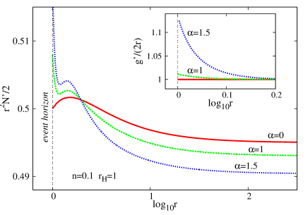
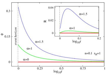
The ECS equations have been solved by using a solver which employs a Newton-Raphson method with an adaptive mesh selection procedure [26], the input parameters being $\{r_{H},n;\alpha\}$. Starting with the GR solutions and slowly increasing $\alpha$, we have found numerical evidence that the NUT metric possesses non-perturbative generalizations in ECS theory. For all considered solutions, the metric functions $N(r),$ $g(r)$ are qualitatively very similar to their $\alpha=0$ counterparts, while the scalar field smoothly interpolate between the asymptotic expansions (4.24), (4.25). To reveal the effects of the CS term, we show in Figure 1 (left) the function $r^{2}N^{\prime}/2$ (whose asymptotic value corresponds to the mass $M$) together with the function $g^{\prime}/(2r)$ (whose values is one in GR). The corresponding scalar field $\phi$ and the Ricci scalar $R$ are shown on the right hand panel of the figure. The solutions there have $r_{H}=1$, $n=0.1$ and several values of $\alpha$.

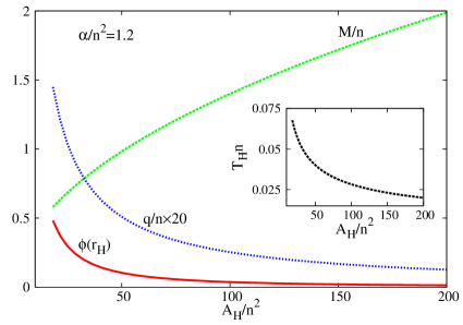
The determination of the domain of existence of the solutions would be a complicated task. In this work we will only report partial results in this direction, by analyzing the pattern of several classes of solutions only. Typical results of the numerical integration are shown in Figure 2 as a function of $\alpha$ (left) and for a varying horizon size (right). Note that all displayed quantities are expressed in units set by the NUT charge $n$, being invariant under the transformation (2.9).

Figure 2: Left: Some parameters of the ECS solutions are shown as a function of $\alpha$ (left) and of the horizon area (right).

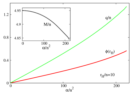
As stated above, the ECS solutions smoothly emerge from the $\alpha=0$ GR ones. At the same time, the numerical results suggest that, for given $(r_{H},n)$, the value of the parameter $\alpha$ cannot be arbitrary large. It turns out that, when the Chern-Simons parameter becomes too large, the scalar field becomes very peaked at the horizon, with large values of the Ricci scalar there, and the overall numerical accuracy strongly decreases. Also, in agreement with the perturbation theory results, the mass $M$ decreases with $\alpha$, while the scalar ‘charge’ $q$ is strictly positive, increasing with $\alpha$.

When varying instead the horizon size for fixed $\{\alpha;n\}$ (Figure 2 (right)), we notice the existence of a minimal value of $A_{H}$, a feature shared with the GR solution. For a given $n$, this minimal value decreases as $\alpha$ increases. Also, the scalar field vanishes gradually for large size of the horizon and becomes peaked at the horizon as the minimal $A_{H}$ is approached.

5 Further remarks. The issue of Taub solution

The main purpose of this work was to investigate the basic properties of the Lorentzian NUT solution in Einstein–Chern-Simons (ECS) theory, viewed as a toy model for a rotating configuration. Even if the primary interest is in the ECS generalization of the Kerr metric (which would possess usual asymptotics and no causal pathologies), we hope that, by widening the context to solutions with NUT charge, one may achieve a deeper appreciation of the model.

The problem has been approached from two different directions: using an expansion in powers of $\alpha$ (the CS coupling constant) around the GR solution, and solving the problem numerically. As expected, our results indicate that the basic properties (in particular the pathologies) of the NUT solution persist for ECS configurations, without spectacular new features. One interesting aspect which deserves further investigation is the possible existence of a maximal value of $\alpha$, as suggested by the numerical results.

Figure 3: The Ricci scalar $R$ and the derivative of the scalar field $\phi^{\prime}$ are shown as a function of $r$, inside and outside the horizon, for two values of $\alpha$ and $r_{H}=1$, $n=0.1$.

This work can be continued in various directions. For example, once the geometry is known, one can study the effects of the CS term on the geodesic motion. In the GR limit, $\alpha=0$, this problem has been extensively discussed in the literature, see $e.g.$ [15], [27]-[32]. Restricting to null circular orbits, one can shown that, for $\sigma(r)=1$, the radius $r=r_{0}>r_{H}$ of the photon sphere is a solution of the equation

$$(N^{\prime}g-Ng^{\prime})|_{r=r_{0}}=0,$$ (5.26)

which in the GR case, reduces to $r_{0}^{3}-3Mr_{0}^{2}-3n^{2}r_{0}+Mn^{2}=0$. For $\alpha\neq 0$, the solution of (5.26) is found numerically. Our results indicate that for a given $n$, the ratio $r_{c}/M$ increases with $\alpha$ (although for all solutions we have considered from this direction, the differences $w.r.t.$ the GR case are at the level of a few percents). It would be interesting to extend this study and to compute $e.g.$ the shadow of the ECS solutions.

Returning to the GR solution (2.10), one remarks that the NUT metric is interesting from yet another point of view. By continuing it through its horizon at $r=r_{H}$ one arrives in the Taub universe, which may be interpreted as a homogeneous, non-isotropic cosmology with an $S^{3}$ spatial topology. (In fact, as discussed by Misner in [13], the NUT spacetime can be joined analytically to the Taub spacetime as a single Taub-NUT spacetime.) Whereas the Schwarzschild solution has a curvature singularity at $r=0$, this is not the case for $n\neq 0$ and the radius coordinate in Taub-NUT (TN) solution may range on the whole real axis.

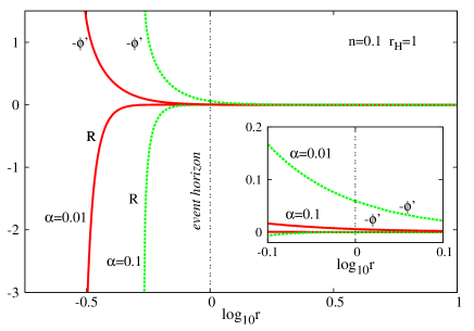
Since the regularity of the TN solution over the whole space-time is somehow exceptional, it is natural to address the question of the behaviour of the ECS solutions inside the horizon. Starting again with a perturbative approach, we remark that the solution derived in Section 3 holds also for $r<r_{H}$. Then one can show that the corrections $N_{2}(r)$ and $\sigma_{2}(r)$ to the TN solution diverge as $1/r^{2}$ as $r\to 0$. As expected, this divergence manifests itself also in the curvature invariants, leading to a divergent character of the solutions, at least to lowest order in perturbation theory.

A similar conclusion is reached when considering a non-perturbative construction of solutions inside the horizon. This is a feasible problem, since we have obtained already the solutions at $r=r_{H}$. This set is used as initial data to integrate inwards, on an interval $[r_{I},r_{H}]$, by decreasing progressively $r_{I}$. The results of the numerical (non-perturbative) integration can be summarized as follows. For all values of the parameters which we have considered, the integration inside can be performed only for $r\in]r_{c},r_{H}]$ with $0<r_{c}<r_{H}$. The minimal value $r_{c}$ depends on the choice of the parameters $\{r_{H},n;\alpha\}$. In particular, the Ricci scalar increases considerably in the limit $r\to r_{c}$, as shown by Figs. 3 (note that a similar picture holds for the Kretschmann invariant $K$). These results strongly suggest that all ECS solutions present an essential singularity at $r=r_{c}$. Unfortunately, we failed to find an analytical argument explaining this feature. However, inspecting the different functions entering in the equations, it turns out that, for the chosen metric gauge, $|\phi^{\prime}(r)|$ strongly increases as $r\to r_{c}$ (see Fig. 3). This induces strong variations of the functions $g^{\prime},g^{\prime\prime}$ and likely leads to the divergence of $R$ and $K$. Finally, let us stress that -in agreement with the perturbative analysis- the critical radius $r_{c}$ decreases towards zero when $\alpha$ decreases. At the same time, its value increases with $\alpha$. Moreover, the existing results suggest that this critical value reaches the horizon radius, $r_{c}\to r_{H}$, as the maximal value of $\alpha$ (noticed in the previous Section) is approached, which would imply a singular horizon in that limit. However, a clarification of these aspects seems to require another parametrization of the problem and possibly a different numerical approach.

One should mention that we have also constructed ECS solutions with a massive scalar field, $V(\phi)=\mu^{2}\phi^{2}/2$. However, all qualitative features of the massless solutions are recovered in that case. In particular, the solution inside the horizon still appears to possess a singularity for a critical value of $r$.

Finally, we remark that it would be interesting to find how a (dynamical) CS term affects the properties of the Euclideanized Taub-NUT solution.

Acknowledgement
E. R. acknowledges funding from the FCT-IF programme. This work was also partially supported by the H2020-MSCA-RISE-2015 Grant No. StronGrHEP-690904, and by the CIDMA project UID/MAT/04106/2013.

References

- [1] R. Jackiw and S. Y. Pi, Phys. Rev. D 68 (2003) 104012 [gr-qc/0308071].
- [2] E. Berti et al., Class. Quant. Grav. 32 (2015) 243001 [arXiv:1501.07274 [gr-qc]].
- [3] S. Alexander and N. Yunes, Phys. Rept. 480 (2009) 1 [arXiv:0907.2562 [hep-th]].
-
[4]
B. A. Campbell, M. J. Duncan, N. Kaloper and K. A. Olive,
Nucl. Phys. B 351 (1991) 778.
B. A. Campbell, M. J. Duncan, N. Kaloper and K. A. Olive, Phys. Lett. B 251 (1990) 34. -
[5]
V. Taveras and N. Yunes,
Phys. Rev. D 78 (2008) 064070
[arXiv:0807.2652 [gr-qc]];
S. Mercuri, Phys. Rev. Lett. 103 (2009) 081302 [arXiv:0902.2764 [gr-qc]]; - [6] A. Ashtekar, A. P. Balachandran and S. Jo, Int. J. Mod. Phys. A 4 (1989) 1493.
- [7] M. Cambiaso and L. F. Urrutia, Phys. Rev. D 82 (2010) 101502 [arXiv:1010.4526 [gr-qc]].
- [8] M. Cambiaso and L. F. Urrutia, arXiv:1008.0591 [gr-qc].
- [9] K. Konno and R. Takahashi, Phys. Rev. D 90 (2014) no.6, 064011 [arXiv:1406.0957 [gr-qc]].
- [10] E. T. Newman, L.Tamburino and T. Unti, J. Math. Phys. 4 (1963) 915.
[11]
M. Damianski and E. T. Newman, Bull. Acad. Pol. Sci,14 (1966) 653;
J. S. Dowker, Gen. Rel. Grav. 5 (1974) 603. - [12] C. W. Misner, in Relativity Theory and Astrophysics I: Relativity and Cosmology, edited by J. Ehlers, Lectures in Applied Mathematics, Volume 8 (American Mathematical Society, Providence, RI, 1967), p. 160.
[13]
C. W. Misner,
J. Math. Phys. 4 (1963) 924;
C. W. Misner and A. H. Taub, Sov. Phys. JETP 28 (1969) 122. - [14] S. W. Hawking in General Relativity. An Einstein Centenary Survey, edited by S. W. Hawking and W. Israel, (Cambridge, Cambridge University Press, 1979) p. 746.
- [15] R. L. Zimmerman and B. Y. Shahir, Gen. Rel. Grav. 21 (1989) 821.
- [16] V. S. Manko and E. Ruiz, Class. Quant. Grav. 22 (2005) 3555 [gr-qc/0505001].
- [17] B. Kleihaus, J. Kunz and E. Radu, Phys. Lett. B 729 (2014) 121 [arXiv:1310.8596 [gr-qc]].
- [18] D. R. Brill, Phys. Rev. 133 (1964) B845.
- [19] E. Radu, Phys. Rev. D 67 (2003) 084030 [hep-th/0211120].
- [20] Y. Brihaye and E. Radu, Phys. Lett. B 615 (2005) 1 [gr-qc/0502053].
- [21] C. V. Johnson and R. C. Myers, Phys. Rev. D 50 (1994) 6512.
[22]
S. Ramaswamy and A. Sen,
J. Math. Phys. 22 (1981) 2612;
A. Magnon, J. Math. Phys. 27 (1986) 1066;
A. Magnon, J. Math. Phys. 28 (1987) 2149. - [23] M. Mueller and M. J. Perry, Class. Quant. Grav. 3 (1986) 65.
- [24] P. Pradhan, Europhys. Lett. 115 (2016) no.3, 30003 [arXiv:1408.2973 [gr-qc]].
- [25] D. Astefanesei, R. B. Mann and C. Stelea, Phys. Rev. D 75 (2007) 024007 [hep-th/0608037].
[26]
U. Ascher, J. Christiansen, R. D. Russell,
Math. Comp. 33 (1979) 659;
U. Ascher, J. Christiansen, R. D. Russell, ACM Trans. 7 (1981) 209. - [27] D. Lynden-Bell and M. Nouri-Zonoz, Rev. Mod. Phys. 70 (1998) 427 [gr-qc/9612049].
- [28] V. Kagramanova, J. Kunz, E. Hackmann and C. Lammerzahl, Phys. Rev. D 81 (2010) 124044 [arXiv:1002.4342 [gr-qc]].
- [29] A. Grenzebach, V. Perlick and C. Lammerzahl, Phys. Rev. D 89 (2014) no.12, 124004 [arXiv:1403.5234 [gr-qc]].
- [30] G. Clément, D. Gal’tsov and M. Guenouche, Phys. Lett. B 750 (2015) 591 [arXiv:1508.07622 [hep-th]].
- [31] P. Pradhan, arXiv:1605.06244 [gr-qc].
- [32] P. Jefremov and V. Perlick, arXiv:1608.06218 [gr-qc].