Baryon interactions in lattice QCD:
the direct method vs. the HAL QCD potential method

Abstract:

We make a detailed comparison between the direct method and the HAL QCD potential method for the baryon-baryon interactions, taking the $\Xi\Xi$ system at $m_{\pi}=0.51$ GeV in 2+1 flavor QCD and using both smeared and wall quark sources. The energy shift $\Delta E_{\mathrm{eff}}(t)$ in the direct method shows the strong dependence on the choice of quark source operators, which means that the results with either (or both) source are false. The time-dependent HAL QCD method, on the other hand, gives the quark source independent $\Xi\Xi$ potential, thanks to the derivative expansion of the potential, which absorbs the source dependence to the next leading order correction. The HAL QCD potential predicts the absence of the bound state in the $\Xi\Xi$(¹S₀) channel at $m_{\pi}=0.51$ GeV, which is also confirmed by the volume dependence of finite volume energy from the potential. We also demonstrate that the origin of the fake plateau in the effective energy shift $\Delta E_{\mathrm{eff}}(t)$ at $t\sim 1$ fm can be clarified by a few low-lying eigenfunctions and eigenvalues on the finite volume derived from the HAL QCD potential, which implies that the ground state saturation of $\Xi\Xi$(¹S₀) requires $t\sim 10$ fm in the direct method for the smeared source on $(4.3\ \mathrm{fm})^{3}$ lattice, while the HAL QCD method does not suffer from such a problem.

1 Introduction

Although Lüscher’s finite volume method [1] and HAL QCD method [2] are theoretically equivalent and employed to study hadron-hadron interactions in lattice QCD [3, 4, 5, 6, 7, 8, 9, 10, 11], two methods give inconsistent results for two-baryon systems (see a review [3]).

Recently, we pointed out that the direct measurement of the two-baryon energy shift in Lüscher’s method suffers from systematic uncertainties due to contamination of excited states [12, 13] that plateaux in the effective energy shift $\Delta E_{\mathrm{eff}}(t)$ disagree between smeared and wall sources. In this talk, we clarify the origin of the fake plateaux in the direct method using the HAL QCD potential, which is insensitive to source operators.

2 Formalism

2.1 Lüscher’s finite volume method

The energy shift of the two-body system in the finite volume $L$, $\Delta E_{\mathrm{BB}}(L)=E_{\mathrm{BB}}(L)-2m_{B}$, with the ground state energy of the two-baryon system $E_{\mathrm{BB}}(L)$ and a single baryon mass $m_{B}$, is related to the phase shift $\delta(k)$ through the finite volume formula [1] as

$$k\cot\delta(k)=\frac{1}{\pi L}\sum_{\vec{n}\in\mathbf{Z}^{3}}\frac{1}{|\vec{n}|^{2}-|kL/(2\pi)|^{2}},$$ (1)

where $k$ is defined by $\Delta E_{\mathrm{BB}}(L)=2\sqrt{(m_{B})^{2}+k^{2}}-2m_{B}$. The bound state is determined from the pole condition, $k\cot\delta(k)=-\sqrt{-k^{2}}$ at $L\rightarrow\infty$ .

In lattice QCD simulations, $\Delta E_{\mathrm{BB}}(L)$ is estimated by the plateau of the effective energy shift

$$\Delta E_{\mathrm{BB}}^{\mathrm{eff}}(t)\equiv E_{\mathrm{BB}}^{\mathrm{eff}}(t)-2m_{\mathrm{B}}^{\mathrm{eff}}(t)=-\frac{1}{a}\log\left(\frac{R_{\mathrm{BB}}(t+a)}{R_{\mathrm{BB}}(t)}\right),$$ (2)

where $R_{\mathrm{BB}}(t)\equiv C_{\mathrm{BB}}(t)/\{C_{\mathrm{B}}(t)\}^{2}$ with the two-baryon propagator $C_{\mathrm{BB}}(t)\equiv\left\langle B(t)^{2}\bar{B}(0)^{2}\right\rangle$, the baryon propagator $C_{B}(t)\equiv\left\langle B(t)\bar{B}(0)\right\rangle$ and the lattice spacing $a$.

2.2 Difficulties in multi-baryon systems

Besides its significant computational cost, the multi-baryon systems in lattice QCD has the signal to noise ratio problem, which becomes exponentially worse for $A$ baryons as $S(t)/N(t)\sim\exp\left[-A(m_{B}-(3/2)m_{M})t\right]$, where $m_{B}$ and $m_{M}$ are the baryon and meson masses. In addition to this, the direct method suffers from the contamination of elastic scattering states, whose energy gap decrease as $\mathcal{O}(1/L^{2})$ as the volume increases. For example, a gap between the ground state and the first $\Xi\Xi$ scattering state is about $50$ MeV at $L=4.3\ \mathrm{fm}$ in this study, which requires $(50\ \mathrm{MeV})^{-1}\ll t\sim\mathcal{O}(10)$ fm for the ground state saturation.

As an instructive example [12] , let us consider the mock-up data as

$$R(t)=b_{1}e^{-\Delta E_{\mathrm{BB}}t}+b_{2}e^{-(\delta E_{\mathrm{el}}+\Delta E_{\mathrm{BB}})t}+c_{1}e^{-(\delta E_{\mathrm{inel}}+\Delta E_{\mathrm{BB}})t},$$ (3)

where $\Delta E_{\mathrm{BB}}=E_{\mathrm{BB}}-2m_{\mathrm{B}}$, while $\delta E_{\mathrm{el}}=E_{\mathrm{BB}}^{\ast}-E_{\mathrm{BB}}$ and $\delta E_{\mathrm{inel}}=E_{\mathrm{inel}}-E_{\mathrm{BB}}$ for the excited states. Fig. 1(a) shows the lines of $\Delta E_{\mathrm{BB}}^{\mathrm{eff}}(t)-\Delta E_{\mathrm{BB}}$ at $\delta E_{\mathrm{el}}=50$ MeV and $\delta E_{\mathrm{inel}}=500$ MeV, which are typical values for the elastic and inelastic excitations, with $c_{1}/b_{1}=0.01$ and $b_{2}/b_{1}=\pm 0.1$, $0$. Without the elastic state ($b_{2}/b_{1}=0$), $\Delta E_{\mathrm{BB}}^{\mathrm{eff}}(t)$ converges to $\Delta E_{\mathrm{BB}}$ around $t\sim 1$ fm within 1 MeV of accuracy, while the ground state saturation requires $t\sim 10$ fm even for the 10% contamination.

Figure 1(b) is the discrete data with fluctuations added. There appear plateau-like structures around $t\sim 1$ fm, which however are fake plateaux as seen in Fig. 1(a). This demonstrates a difficulty in obtaining the ground state energy from a plateau-like structure in $\Delta E_{\mathrm{eff}}(t)$ at $t\simeq 1$ fm.

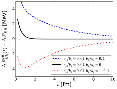
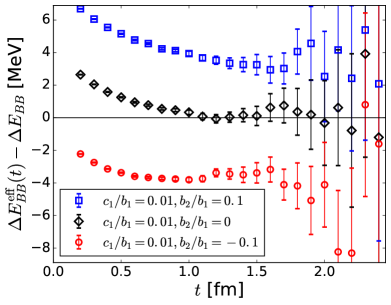
Figure 1: (a) The effective energy shift of the mock-up data. (b) A mock-up data with fluctuations.

2.3 HAL QCD method

Contrary to the direct method, the time-dependent HAL QCD method [9] utilizes all scattering state below the inelastic threshold to extract the non-local potential $U(\vec{r},\vec{r}^{\prime})$ as

$$\left[\frac{1}{4m_{B}}\frac{\partial^{2}}{\partial t^{2}}-\frac{\partial}{\partial t}-H_{0}\right]R(\vec{r},t)=\int d\vec{r}^{\prime}U(\vec{r},\vec{r}^{\prime})R(\vec{r}^{\prime},t)$$ (4)

for $t\gg(\Delta W_{\mathrm{th}})^{-1}$, where the Nambu-Bethe-Salpeter (NBS) correlation function $R(\vec{r},t)$ is defined as

$$R(\vec{r},t)\equiv\left\langle 0|T\{B(\vec{x}+\vec{r},t)B(\vec{x},t)\bar{\mathcal{J}}(0)|0\right\rangle/\{C_{B}(t)\}^{2}=\sum_{n}A_{n}\phi^{W_{n}}(\vec{r})e^{-\Delta W_{n}t}+\mathcal{O}(e^{-\Delta W_{\mathrm{th}}t})$$ (5)

with a source operator $\mathcal{J}$, $\Delta W_{n}=W_{n}-2m_{B}$ with $n$-th energy eigenvalue $W_{n}$, and the inelastic threshold $\Delta W_{\mathrm{th}}=W_{\mathrm{th}}-2m_{B}$. Using the velocity expansion, $U(\vec{r},\vec{r}^{\prime})\simeq\{V(\vec{r})+\mathcal{O}(\nabla^{2})\}\delta(\vec{r}-\vec{r}^{\prime})$, the leading order potential is given by

$$V(\vec{r})=\frac{1}{4m_{B}}\frac{(\partial/\partial t)^{2}R(\vec{r},t)}{R(\vec{r},t)}-\frac{(\partial/\partial t)R(\vec{r},t)}{R(\vec{r},t)}-\frac{H_{0}R(\vec{r},t)}{R(\vec{r},t)}.$$ (6)

3 Lattice QCD measurements for $\Xi\Xi$ interactions

We use 2+1 flavor QCD ensembles in Ref. [6], generated with the Iwasaki gauge action and $\mathcal{O}(a)$-improved Wilson quark action at $a=0.8995(40)$ fm, where $m_{\pi}=0.51$ GeV, $m_{N}=1.32$ GeV and $m_{\Xi}=1.46$ GeV. For a comparison, we employ the wall source $q^{\mathrm{wall}}(t)=\sum_{\vec{y}}q(\vec{y},t)$, which is mainly used in the HAL QCD method, as well as the smeared source $q^{\mathrm{smear}}(\vec{x},t)=\sum_{\vec{y}}f(|\vec{x}-\vec{y}|)q(\vec{y},t)$ with $f(r)\equiv Ae^{-Br},1,0$ for $0<r<(L-1)/2$, $r=0$, $(L-1)/2\leq r$, which is generally adopted for the direct method. Simulation parameters including $(A,B)$ identical to those in Ref. [6] are summarized in Table 1. In this report, we mainly consider $\Xi\Xi$(¹S₀) channel using the relativistic interpolating operators, since $\Xi\Xi$(¹S₀) channel has smaller statistical errors but belongs to the same SU(3) flavor representation of the NN(¹S₀).

3.1 Quark source dependence of the effective energy shift $\Delta E_{\Xi\Xi}^{\mathrm{eff}}(t)$

Quark source dependence is an easy check against fake plateaux. We compare the effective energy shift between the wall and smeared sources in Fig. 2 for $\Xi\Xi$(¹S₀) (Left) and $\Xi\Xi$(³S₁) (Right) on $48^{3}$ lattice. While plateau-like structures appear around $t=15a$ for both sources, they disagree with each other, implying that either plateau (or both) is fake. Repeating this analysis on other volumes and taking $L\rightarrow\infty$ limit, we have found that the lowest energy state from the wall source is the scattering state in both $\Xi\Xi$(¹S₀) and $\Xi\Xi$(³S₁) channels, while that from the smeared source turns out to be the bound state in the $\Xi\Xi$(¹S₀) channel but an unphysical state in the $\Xi\Xi$(³S₁), which has positive energy shift $\Delta E_{\mathrm{\Xi\Xi}}(^{3}$S${}_{1})>0$ in the infinite volume limit. These results bring serious doubt on the validity of the energy shift in the previous works [6, 7, 8] . More detailed studies including NN, ³He and ⁴He systems are found in Ref. [12].

volume	$La$	# of conf.	# of smeared sources	$(A,B)$	# of wall sources
$32^{3}\times 48$	2.9 fm	402	384	$(1.0,0.18)$	48
$40^{3}\times 48$	3.6 fm	207	512	$(0.8,0.22)$	48
$48^{3}\times 48$	4.3 fm	200	$4\times 384$	$(0.8,0.23)$	$4\times 48$
$64^{3}\times 64$	5.8 fm	327	$1\times 256$	$(0.8,0.23)$	$4\times 64$

Table 1: Simulation parameters. The rotational symmetry for isotropic lattice is used to increase statistics.

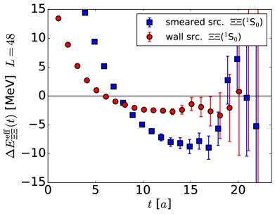
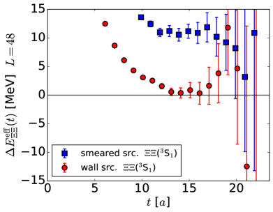
Figure 2: Examples of the effective energy shift plots at $L^{3}=48^{3}$.

3.2 Quark source dependence of the HAL QCD potential

We similarly consider the source dependence of the HAL QCD potential. Fig. 3(a) and (b) show the central potential $V_{C}(r)$ of $\Xi\Xi$(¹S₀) at $L^{3}=48^{3}$ from smeared and wall sources, respectively. While $V_{C}^{\mathrm{wall}}(r)$ is stable against a variation of $t$ from $t=11a$ to $15a$ within errors, $V_{C}^{\mathrm{smear}}(r)$ has a weak $t$ dependence and is slightly different from $V_{C}^{\mathrm{wall}}(r)$ as seen in Fig. 3(c) at $t=15a$ though the difference decreases as $t$ increases.

Contrary to the direct method, the source dependence in the HAL QCD method give an extra information, from which we can determine the next leading order of the derivative expansion as

$$V^{X}_{C}(r)R^{X}(r,t)\equiv\left[\frac{1}{4m}\frac{\partial^{2}}{\partial t^{2}}-\frac{\partial}{\partial t}-H_{0}\right]R^{X}(r,t)=V_{\mathrm{LO}}(r)R^{X}(r,t)+V_{\mathrm{NLO}}(r)\nabla^{2}R^{X}(r,t)$$ (7)

with $X=$ wall, smeared. As seen in Fig. 3 (d), $V_{C}^{\mathrm{wall}}(r)$ is a good approximation of $V_{\mathrm{LO}}(r)$, so that it gives reliable results at the low energy where $V_{\mathrm{LO}}(r)$ dominates.

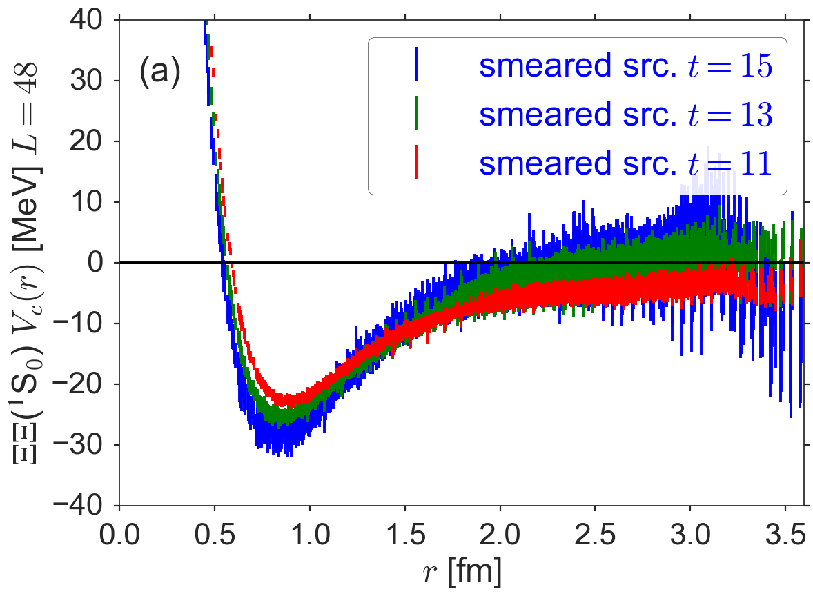
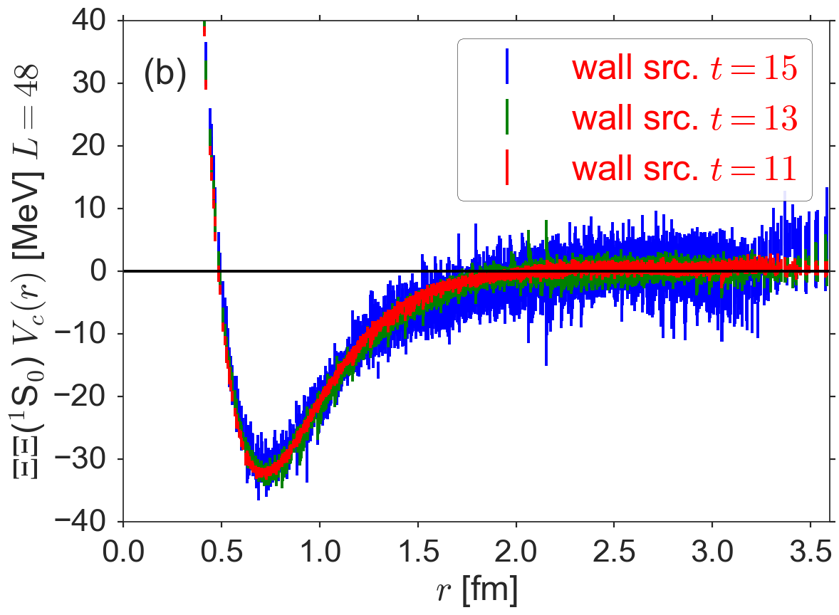
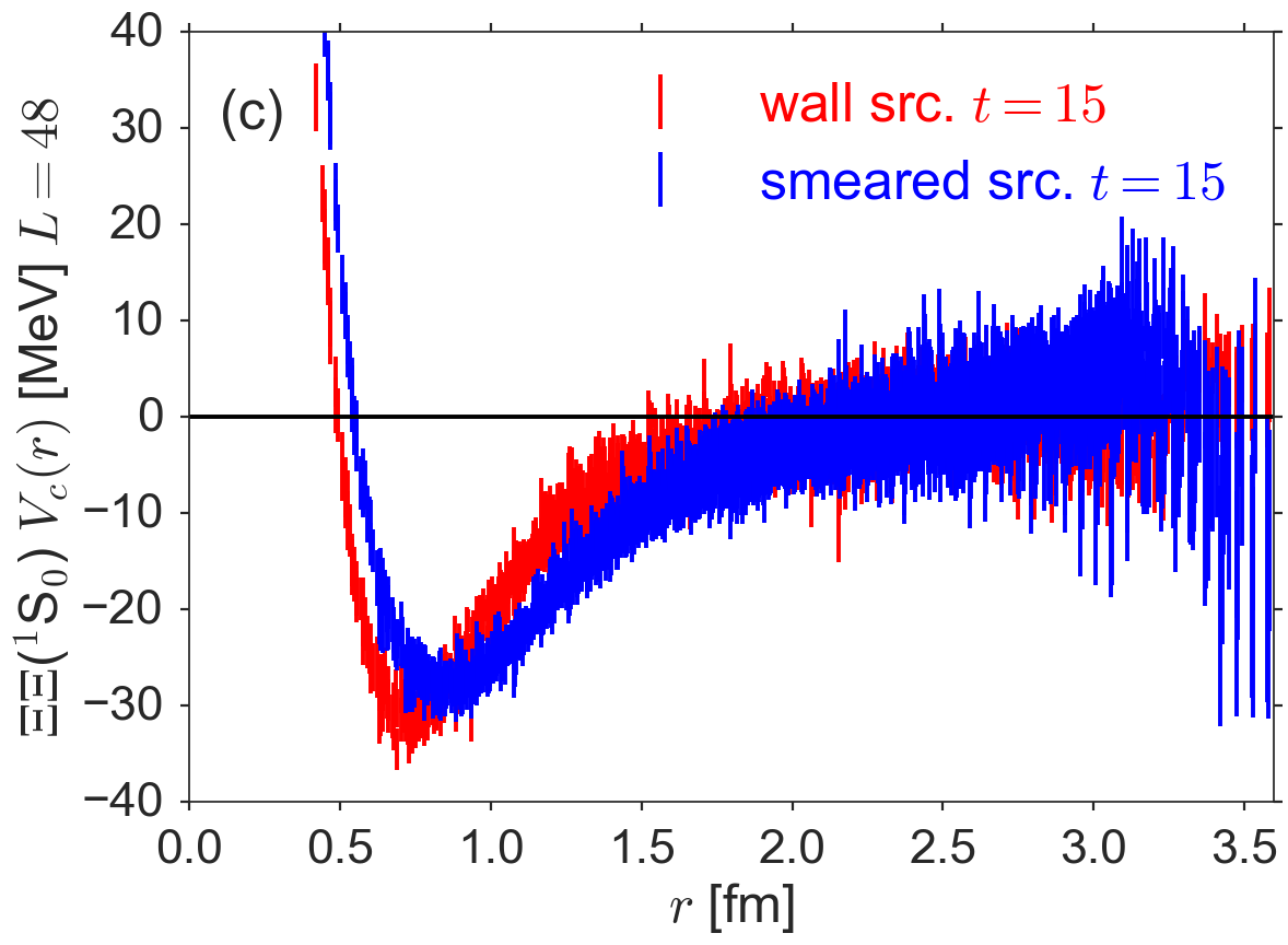
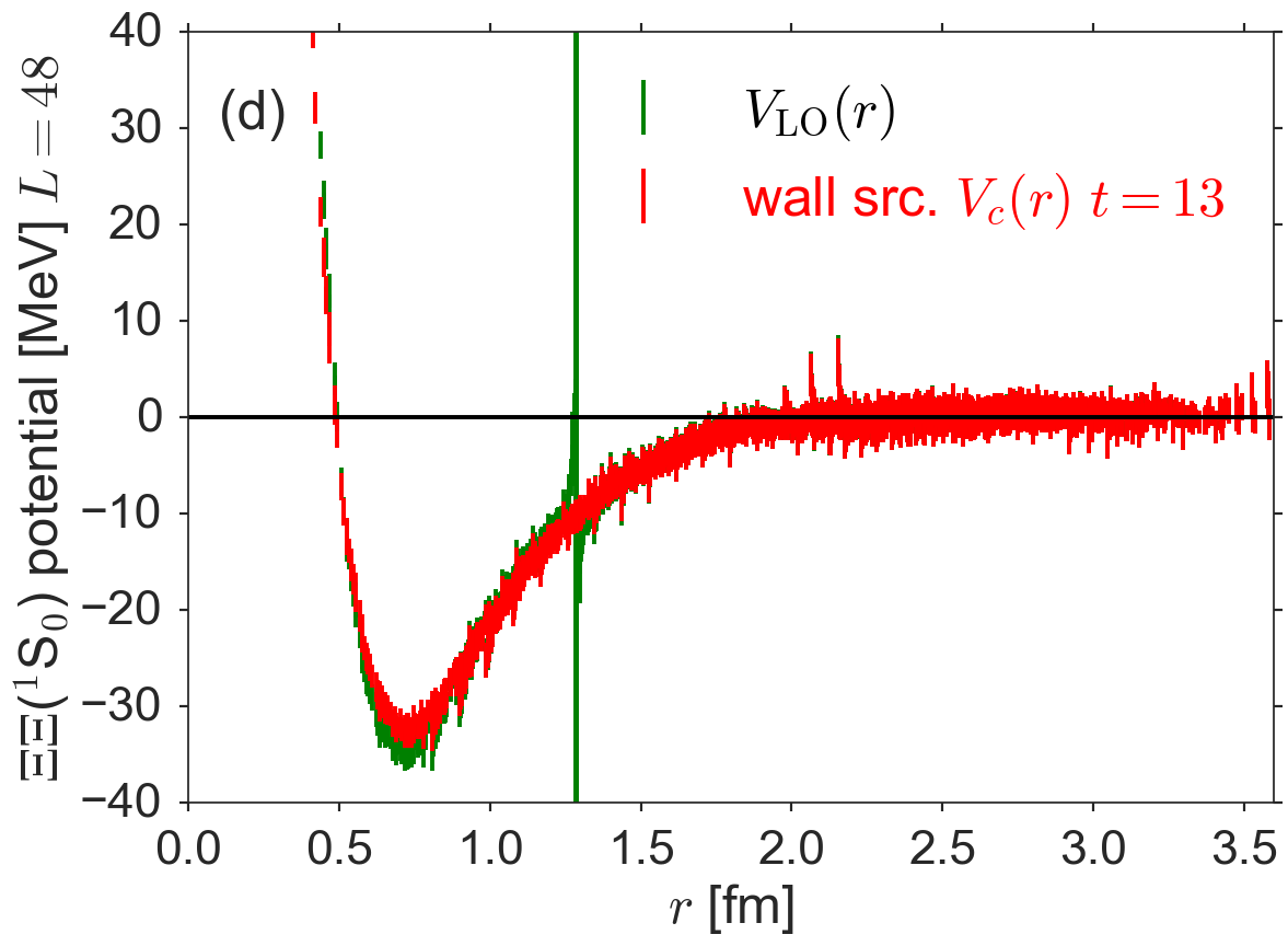
Figure 3: $V_{C}(r)$ of $\Xi\Xi$(¹S₀) for $L^{3}=48^{3}$. (a) $V_{C}^{\mathrm{smear}}(r)$ at $t=11,13$ and $15$ (b) $V_{C}^{\mathrm{wall}}(r)$ at $t=11$, $13$ and $15$. (c) a comparison between $V_{C}^{\mathrm{wall}}(r)$ and $V_{C}^{\mathrm{smear}}(r)$ at $t=15$. (d) LO potential $V_{\mathrm{LO}}(r)$ and $V_{C}^{\mathrm{wall}}(r)$.

3.3 Anatomy of fake plateaux by the potential

While we have found no bound state in $\Xi\Xi(^{1}$S₀) channel from the Shrödinger equation with the HAL QCD potential in the infinite volume, eigenvalues of $H=H_{0}+V$ on the finite volume $L$ gives the finite volume ground state energy [10, 13]. Fig. 4(a) shows the volume dependence of the lowest eigenvalue $\Delta E_{0}$ for $L^{3}=40^{3},48^{3}$ and $64^{3}$ from the wall source potential $V_{C}^{\mathrm{wall}}(r)$ at $t=14a$ , together with the linear extrapolation in $1/L^{3}$, which confirms the absence of the bound state in the $\Xi\Xi(^{1}$S₀) at $m_{\pi}=0.51$ GeV.

Furthermore, using several low-lying eigenfunctions $\Psi_{n}(\vec{r})$ with eigenvalues $\Delta E_{n}$, we can decompose $\Xi\Xi$ correlation functions as

$$\sum_{\vec{r}}R^{\mathrm{wall/smear}}(\vec{r},t)\simeq\sum_{\vec{r}}\sum_{n}a_{n}^{\mathrm{wall/smear}}\Psi_{n}(\vec{r})\exp\left(-\Delta E_{n}t\right)=\sum_{n}b_{n}^{\mathrm{wall/smear}}\exp\left(-\Delta E_{n}t\right),$$ (8)

where $a_{n}^{\mathrm{wall/smear}}$ are determined from the orthogonality of $\Psi_{n}(\vec{r})$. Fig. 4(b) shows the ratio $|b_{n}/b_{0}|$ as a function of the eigenvalue $\Delta E_{n}$, which shows that the contamination of excited states. The contamination from the first excitation with about 50 MeV at $L^{3}=48^{3}$ is much smaller than 1% for the wall source, while it is about 10% for the smeared source.

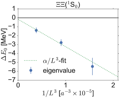
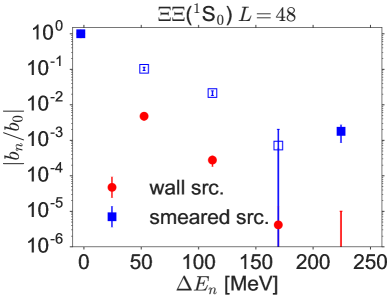
Figure 4: (a) The volume dependence of the ground state eigenvalue $\Delta E_{0}$. (b) The contamination of excited states $|b_{n}/b_{0}|$. Solid (open) symbol denotes a positive(negative) value.

Using the decomposition Eq. (8), we can reconstruct the effective energy shift $\Delta E_{\mathrm{eff}}(t)$, as shown in Fig. 5 (Left), where the reconstructed result, denoted by the gray (orange) band for the wall (smeared) source is compared with the direct calculation. The plateau-like structure for both sources is well explained by the reconstruction, while it is also shown that the ground saturation for the smeared source requires $t\sim 100a\simeq 10$ fm [12].

The effective energy from $\sum_{\vec{r}}g(r)R^{\rm smeared}(\vec{r},t)$ is plotted in Fig. 5 (Right), which shows the strong sink operator dependence among $g(r)=1$ (solid square), $g_{1}(r)$ (open square) and $g_{2}(r)$ (open diamond), while we confirm the agreement among three for the wall source[12].

Plateaux of the effective energy shift from $\sum_{\vec{r}}\Psi_{0}(\vec{r})R^{\rm wall/smeared}(\vec{r},t)$, where $\Psi_{0}(\vec{r})$ is the lowest eigenstate at $t=14a$ on $L=48$, on the other hand, agree between the wall (open down triangle) and the smeared (open up triangle) sources in Fig. 5 (Right), where they also agree with that from the wall source without $\Psi_{0}(r)$ (solid circle). This analysis demonstrates that the lowest eigenstate from the potential is indeed correct, and one can extract the correct lowest energy in the direct method once we know the eigenstate. In the present case, the wall source happens to give the correct lowest energy within errors in the direct method, though this is not always the case.

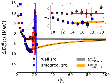
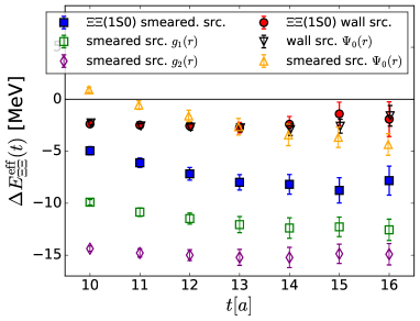
Figure 5: (Left) Reconstructions of $\Delta E_{\mathrm{eff}}(t)$ from low-lying three eigenstates. (Right) Effective energy shift from sink projection by $g_{1}(r)=1-0.5e^{-0.2r}$, $g_{2}(r)=1-0.9e^{-0.22r}$ and $\Psi_{0}$.

We have shown that the direct measurement for the energy shift has strong source and sink dependencies while the (time-dependent) HAL QCD method is free from these dependencies. We also demonstrate that the origin of the fake plateau of the effective energy shift in the direct method can be clarified by the lowest few eigenstates by using the potential on the finite volume.

We thank the authors of [6] for providing the gauge configurations and the detailed account of the smeared source used in [6]. The lattice QCD calculations have been performed on Blue Gene/Q at KEK (Nos. 12/13-19, 13/14-22, 14/15-21, 15/16-12), HA-PACS at University of Tsukuba (Nos. 13a-23, 14a-20) and K computer at AICS (hp150085, hp160093). This research was supported by MEXT as “Priority Issue on Post-K computer” (Elucidation of the Fundamental Laws and Evolution of the Universe) and JICFuS.

References

- [1] M. Lüscher, Nucl. Phys. B 354, 531 (1991).
- [2] N. Ishii, S. Aoki and T. Hatsuda, Phys. Rev. Lett. 99 (2007) 022001 [nucl-th/0611096].
- [3] T. Yamazaki, PoS LATTICE 2014 (2015) 009 [arXiv:1503.08671 [hep-lat]], and the references therein.
- [4] S. Aoki et al. [HAL QCD Collaboration], PTEP 2012 (2012) 01A105 [arXiv:1206.5088 [hep-lat]].
- [5] T. Kurth, N. Ishii, T. Doi, S. Aoki and T. Hatsuda, JHEP 1312 (2013) 015 [arXiv:1305.4462 [hep-lat], arXiv:1305.4462].
- [6] T. Yamazaki, K. i. Ishikawa, Y. Kuramashi and A. Ukawa, Phys. Rev. D 86 (2012) 074514 [arXiv:1207.4277 [hep-lat]];
- [7] T. Yamazaki, K. i. Ishikawa, Y. Kuramashi and A. Ukawa, Phys. Rev. D 92 (2015) 1, 014501 [arXiv:1502.04182 [hep-lat]].
- [8] S. R. Beane et al. [NPLQCD Collaboration], Phys. Rev. D 85 (2012) 054511 [arXiv:1109.2889 [hep-lat]]; Phys. Rev. D 87 (2013) 3, 034506 [arXiv:1206.5219 [hep-lat]]; Phys. Rev. C 88 (2013) 2, 024003 [arXiv:1301.5790 [hep-lat]].
- [9] N. Ishii et al. [HAL QCD Collaboration], Phys. Lett. B 712 (2012) 437 [arXiv:1203.3642 [hep-lat]].
- [10] B. Charron [HAL QCD Collaboration], PoS LATTICE 2013 (2014) 223 [arXiv:1312.1032 [hep-lat]].
- [11] M. Yamada et al. [HAL QCD Collaboration], PTEP 2015 (2015) 7, 071B01 [arXiv:1503.03189 [hep-lat]].
- [12] T. Iritani et al., JHEP 1610 (2016) 101 [arXiv:1607.06371 [hep-lat]].
- [13] T. Iritani [HAL QCD Collaboration], PoS LATTICE 2015 (2016) 089 [arXiv:1511.05246 [hep-lat]].
- [14] S. Aoki, PoS LATTICE 2016 (2016) 109 [arXiv:1610.09763], and in preparation.