On the radial velocity detection of additional planets in transiting, slowly rotating M-dwarf systems: the case of GJ 1132

Abstract

M-dwarfs are known to commonly host high-multiplicity planetary systems. Therefore M-dwarf planetary systems with a known transiting planet are expected to contain additional small planets ($r_{p}\leq 4$ R_⊕, $m_{p}\lesssim 20$ M_⊕) that are not seen in transit. In this study we investigate the effort required to detect such planets using precision velocimetry around the sizable subset of M-dwarfs which are slowly rotating ($P_{\mathrm{rot}}\gtrsim 40$ days) and hence more likely to be inactive. We focus on the test case of GJ 1132. Specifically, we perform a suite of Monte-Carlo simulations of the star’s radial velocity signal featuring astrophysical contributions from stellar jitter due to rotationally modulated active regions and keplarian signals from the known transiting planet and hypothetical additional planets not seen in transit. We then compute the detection completeness of non-transiting planets around GJ 1132 and consequently estimate the number of RV measurements required to detect those planets. We show that with 1 m s^-1 precision per measurement, only $\sim 50$ measurements are required to achieve a 50% detection completeness to all non-transiting planets in the system and to planets which are potentially habitable. Throughout we advocate the use of Gaussian process regression as an effective tool for mitigating the effects of stellar jitter including stars with high activity. Given that GJ 1132 is representative of a large population of slowly rotating M-dwarfs, we conclude with a discussion of how our results may be extended to other systems with known transiting planets such as those which will be discovered with TESS.

1. Introduction

One major endeavour in current exoplanet research is the characterization of exoplanetary atmospheres through spectroscopic investigation. Indeed such efforts have already been performed from the ground as well as from space-based observatories including the Hubble Space Telescope and Spitzer Space Telescope, on primarily transiting giant planets (Bean et al., 2013; Crouzet et al., 2014; McCullough et al., 2014) and even on planets down to $\sim 3$ Earth radii (Kreidberg et al., 2014). High-dispersion spectroscopy may also be used to characterize non-transiting exoplanet atmospheres including measurements of orbital inclinations and planetary rotation velocities (Snellen, 2013). With upcoming technological advances on-board the James Webb Space Telescope, researchers in the field are pushing the boundary towards the characterization of exoplanetary atmospheres around planets with bulk Earth-like compositions (Beichman et al., 2014). Such experiments require nearby planetary systems and favors hot planets around small host stars wherein the atmospheric transmission signal is maximized (Brown, 2001). Therefore the most favorable targets for characterizing potential Earth-like exoplanetary atmospheres are around nearby M-dwarf stars.

Numerous current and upcoming transiting exoplanet missions (e.g. K2, TESS, CHEOPS) will discover nearby M-dwarf transiting planetary systems which are sufficiently bright and are therefore amenable to atmospheric characterization. For example, the upcoming Transiting Exoplanet Survey Satellite mission (Ricker et al., 2014) is expected to detect $\sim 980$ transiting planets around M-dwarfs ($T_{\mathrm{eff}}\leq 3800$ K) including $\sim 50$ bright M-dwarfs with $J<9.5$ (Sullivan et al., 2015). Given the high frequency of Earth to mini-Neptune sized planets around early-mid M-dwarfs ($\sim 0.36-2.5$ planets per M-dwarf; Bonfils et al., 2013; Dressing & Charbonneau, 2015; Gaidos et al., 2016), including planets within the habitable zone, many of these newly discovered transiting M-dwarf planetary systems will contain additional planets not seen in transit but are potentially detectable with radial velocity (RV) follow-up observations. It is therefore of interest to observers conducting such observations of these systems to quantify the effort which is required to detect these additional ‘non-transiting’ planets and obtain accurate measurements of all planet masses.

Unfortunately, RV observations are often deterred by strong RV jitter signals (Wright, 2005) associated with magnetic regions which, for M-dwarfs, tend to be strongest on stars undergoing rapid rotation (Mohanty & Basri, 2003; Browning et al., 2010; Reiners et al., 2012; West et al., 2015). For M-dwarfs, empirically there exist two populations of rotation periods (e.g. Irwin et al., 2011; McQuillan et al., 2013a, 2014; Newton et al., 2016b) with a significant subset of M-dwarfs having rotation periods $\gtrsim 40$ days. These slowly rotating stars are expected to have low levels of rotationally-induced stellar jitter from active regions such as spots and plages (Aigrain et al., 2012) compared to their rapidly rotating counterparts. For example, the slowly rotating M-dwarfs GI 176 and GI 674 ($P_{\mathrm{rot}}=39$ and 35 days respectively) have been shown to exhibit comparatively small levels of activity jitter with an amplitude of $\sim 5$ m s^-1 (Bonfils et al., 2007; Forveille et al., 2009). The typical low-amplitude jitter thus makes slow rotators attractive targets for the atmospheric characterization of their planetary companions and detection of additional planets not seen in transit, both of which are strongly deterred by stellar jitter. Rapid rotators are made additionally disfavorable for RV measurements as the intrinsic Doppler broadening of spectral features significantly degrades the RV accuracy thus making the determination of planetary masses less precise.

In this study we investigate the observational effort required to detect additional planets in transiting M-dwarf planetary systems, focusing on the subset of M-dwarfs which are slowly rotating and are therefore less likely to be magnetically active. We address this problem using the GJ 1132 planetary system as a fiducial test case. We do so by modelling the observed photometric variability of GJ 1132 in order to model the corresponding RV jitter from rotationally modulated active regions. We then perform a suite of Monte-Carlo realizations of simulated RV timeseries which sample from the known population of small planets around M-dwarfs and compute the detection completeness of those planets under realistic observing conditions. A direct consequence of this calculation provides limits on the number of RV observations required to recover additional planets around slowly rotating M-dwarfs such as GJ 1132.

In Sect. 2 we briefly summarize the current state of knowledge of GJ 1132 and GJ 1132b. In Sect. 3 we present the details of our Monte-Carlo simulations, Sect. 4 presents the resulting detection completeness of small planets around GJ 1132 followed in Sect. 5 by a discussion of our assumptions and the broad applicability of our results to similar planetary systems such as those which will be discovered with TESS. A summary of our results is presented in Sect. 6 for ease of reference.

2. GJ 1132 Planetary System

The GJ 1132 planetary system (M4.5V, $V=13.49$, $J=9.25$; Berta-Thompson et al., 2015, hereafter B15) is the most recent planet discovery from the MEarth transiting planet survey (Irwin et al., 2015). At just 12 pc, the planet known as GJ 1132b is currently one of the closest transiting rocky exoplanets to the solar system. GJ 1132b is slightly larger than the Earth and has an orbital period of less than 2 days, placing it interior to its host star’s habitable zone. Photometric and RV measurements determined that the planet has a rocky bulk composition (B15). Together, this has lead to claims that GJ 1132b might represent a Venus analog (low water vapor mass fraction as a result of thermal escape) but requires atmospheric characterization via spectroscopic follow-up to probe the planet’s atmosphere and challenge that notion. Owing to the planetary system’s close proximity, GJ 1132b represents a very appealing target for the atmospheric characterization of a rocky exoplanet with JWST.

As discussed in the introduction, this single planetary system should host additional planets not seen in transit which could potentially exist within the star’s habitable zone between $\approx 15-39$ days (Kopparapu et al., 2013). Scrutinous photometric monitoring and a modest RV timeseries did not reveal the presence of any additional planets (B15 and this work. See Sect. 3.4.1 and Table 2). Although any planets co-planar with GJ 1132b, but with $a/R_{s}\gtrsim 42$, would not transit. For reference, $a/R_{s}=16$ for GJ 1132b.

The planet discovery paper presented multiple transit observations and measured a planetary radius of GJ 1132b of 1.16 R_⊕. RV measurements taken with the HARPS spectrograph (Mayor et al., 2003) also revealed a $3\sigma$ mass detection of 1.62 M_⊕ thus giving GJ 1132b a bulk density consistent with a rocky, Earth-like composition. Additionally, B15 presented a long baseline stellar light curve for which a stellar rotation period of $\sim 125$ days was inferred. From this slow rotation period one expects a correspondingly low level of stellar jitter (Aigrain et al., 2012) which is greatly beneficial for the detection of additional planetary companions with RVs. The properties of GJ 1132 and GJ 1132b are summarized in Table 1.

Table 1GJ 1132 Planetary System Properties

Parameter	B15 Value	Value from this work
GJ 1132 (star)
Stellar Mass, $M_{s}$	$0.181\pm 0.019$ M⊙	-
Stellar Radius, $R_{s}$	$0.207\pm 0.016$ R⊙	-
Effective Temperature, $T_{\mathrm{eff}}$	$3270\pm 140$ K	-
Stellar Luminosity, $L_{s}$	$(4.38\pm 0.34)\times 10^{-3}$ L⊙	-
Stellar Age	$>5$ Gyrs	-
Rotation Period, $P_{\mathrm{rot}}$	125 days	$122.31^{+6.03}_{-5.04}$ days
GJ 1132b (planet)
Orbital Period, $P_{b}$	$1.62893\pm 3.1\times 10^{-5}$ days	-
Time of Mid-Transit, $T0_{b}$	$2457184.55786\pm 0.00032$ BJD	-
Planetary Radius, $r_{p,b}$	$1.16\pm 0.11$ R⊕	-
Eccentricity, $e_{b}$	0	-
Inclination, $i_{b}$	$88.63\pm 0.86^{\circ}$	-
Semiamplitude, $K_{b}$	$2.76\pm 0.92$ m s-1	$2.69^{+0.81}_{-0.79}$ m s-1
Planetary Mass, $m_{p,b}$	$1.62\pm 0.55$ M⊕	$1.58^{+0.49}_{-0.48}$ M⊕

3. Monte-Carlo Simulations

To determine the detection completeness of small ($\leq 4$ R_⊕) planets around GJ 1132 with dedicated RV follow-up, here we run an extensive Monte-Carlo (MC) simulation of planetary systems (including GJ 1132b) around GJ 1132. When constructing RV timeseries and searching for additional planets we fully exploit the available data for this system described in Sect. 2 which includes a model of the RV jitter derived from the star’s photometric light curve. The setup of our MC simulation is described in the proceeding sections.

3.1. Modelling Radial Velocity Jitter from MEarth Photometry

3.1.1 Gaussian process photometry model

The rotation of active regions such as spots and plages in the stellar photosphere of GJ 1132 gives rise to RV jitter which varies with time. The long-baseline photometric light curve presented in B15 (planetary transits are removed) provides the opportunity to model this source of astrophysical noise empirically. In brief, this is done by modelling the photometric light curve with a smoothly varying function which is then used to predict the associated RV signal from the active regions presumed responsible for the observed photometric variability. Because the transits of GJ 1132b have been removed from the light curve, the observed photometric variability can be solely attributed to active regions on the star. Therefore unlike the observed RVs which contain signals from GJ 1132b and possibly from additional, non-transiting planets, the light curve traces the source of stellar jitter only. The light curve and best-fit model, shown in Fig. 1, are described in the proceeding paragraphs.

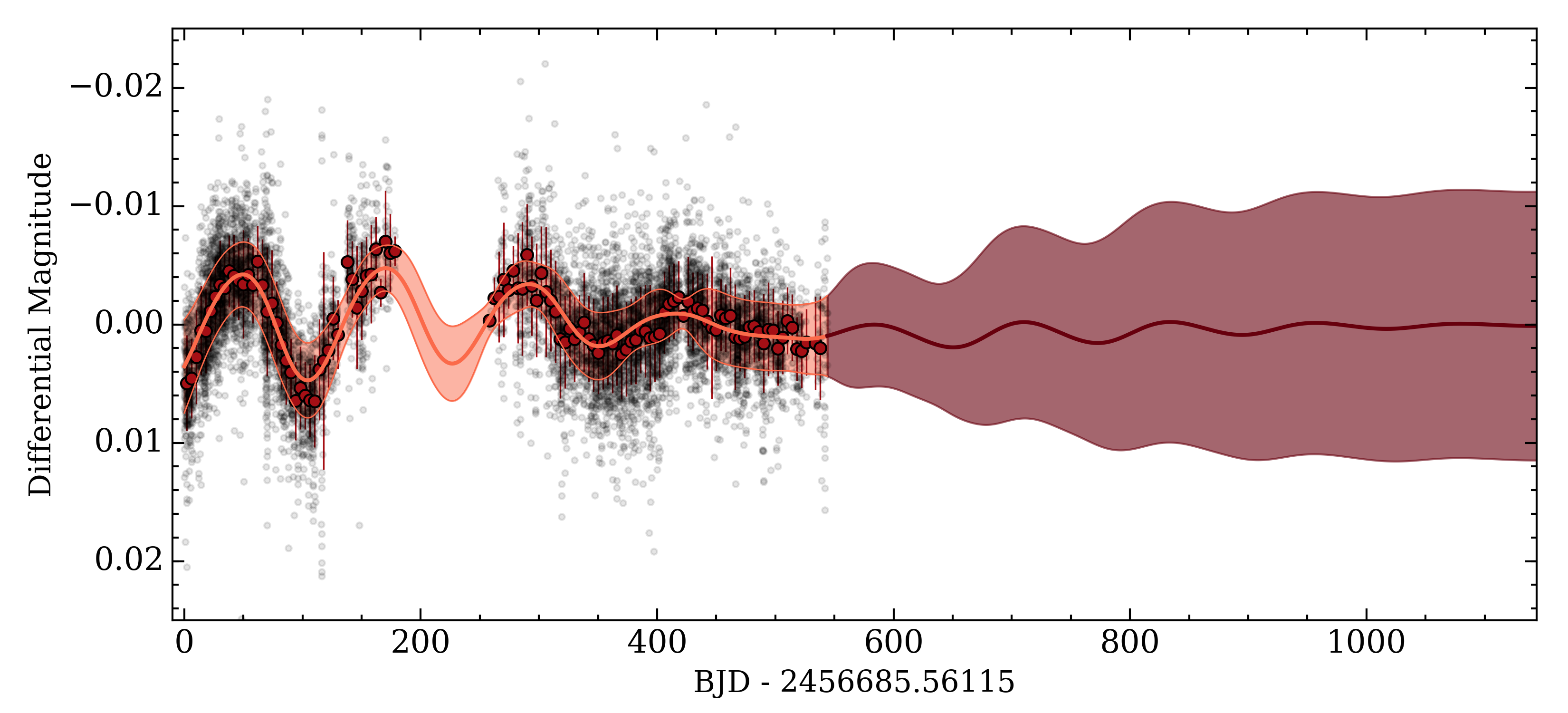
Figure 1.— The MEarth photometry originally presented in B15. Red dots are the binned photometric measurements modelled with a quasi-periodic Gaussian process (GP) which reveals a stellar rotation period of $\sim 122$ days. The mean GP model and 99% confidence intervals are shown in pink. The GP predictive light curve and 99% confidence intervals are shown for 600 days following the last photometric observation in red.

The photometric data of GJ 1132 were obtained with the MEarth-South telescope array at the Cerro Tololo Inter-American Observatory (CTIO) in Chile between January 2014 and July 2015. The systematic effects unique to the MEarth telescopes have been corrected for and are described in detail in Newton et al. (2016b). This includes the removal of the ‘common-mode’ systematic effect resulting from atmospheric extinction due to telluric water vapor absorption in the MEarth bandpass. We proceed using the fully reduced photometry following a clip of ‘bad’ photometric points corresponding to frames with an uncharacteristically low zero-point magnitude correction possibly resulting from cloud cover.

Due to complexities regarding the differential rotation of the stellar photosphere and variations in the sizes and contrast of multiple active regions on the stellar surface, the photometric variability need not be strictly periodic. We note that for mid M-dwarfs such as GJ 1132, the effect of differential rotation may vanish or at least be small due to the extensive convective depth (Barnes et al., 2005). Additionally, parametric models of stellar variability due to active regions feature degenerate model parameters including the sizes and spatial distribution of active regions thus making it difficult to accurately constrain model parameters of active regions. We instead opt to model the photometric variability of GJ 1132 using non-parametric Gaussian process (GP) regression. A discussion of the full Gaussian process formalism is presented in appendix A for the interested reader. Most crucially, by assuming that photometric measurements are correlated in time via the rotation of the star, we model the covariance between photometric measurements with a GP specified by a null mean function and a covariance function which varies quasi-periodically (Eq. A1).

The photometry shown in Fig. 1 is accompanied by the mean of the GP predictive distribution and its $99$% confidence interval. We then use the GP predictive distribution to predict the photometric variability for 600 days following the last available photometric measurement.

3.1.2 Radial velocity jitter model

From the photometry, the corresponding RV signal or astrophysical jitter can be approximately estimated. Haywood et al. (2016) used contemporaneous RV measurements and images of the Sun to argue that photometry is an incomplete diagnostic of the RV jitter from active regions. Yet the photometric light curve still gives approximate empirical insight into the nature of the star’s RV jitter arising from active regions. The conversion to RV from photometry is done using the analytical $FF^{\prime}$ method from Aigrain et al. (2012) which uses the time-varying fractional coverage of the stellar disk by active regions and it first time derivative to model the corresponding RV variations. Due to the smoothness of the GP model of the light curve we are able to compute the time derivative of the star’s fractional spot coverage in a simplistic way using finite differences. Specifically, we use the python numpy.gradient function; an accurate second-order forward/backwards scheme to estimate the time derivative at the boundaries and a central differences scheme elsewhere.

This jitter model does not consider certain higher order effects such as granulation and stellar oscillation modes whose amplitudes are each seen to diminish with later spectral types (Christensen-Dalsgaard, 2004; Gray, 2009; Dumusque et al., 2011) and we assume can be averaged down using long integration times (Lovis et al., 2005). Furthermore, we do not include the jitter arising from the Zeeman broadening of spectral features in the presence of magnetic fields (Reiners et al., 2013) because empirical correlations between the stellar rotation period and magnetic field strength indicate that slow rotators, such as GJ 1132, have a negligible contribution to the RV jitter from Zeeman broadening (Reiners & Basri, 2007; West et al., 2015) even at near-IR wavelengths where the effect is stronger than in the optical (Reiners et al., 2013). We also neglect flares in our jitter model because their distinctive spectral signature allows them to be easily flagged and removed from the RV timeseries (Schmidt et al., 2012).

The modelled contributions to the RV jitter from the $FF^{\prime}$ method result from the superposition of two effects: i) the suppression of particularly Doppler-shifted flux from the occultation of the differentially Doppler-shifted stellar limbs by active regions traversing the stellar disk (the flux effect) and ii) from the suppression of the convective blueshift at the photospheric boundary as the fractional spot coverage evolves with time. Focusing on the latter effect, the convective blueshift term scales directly with the velocity difference between the active regions and the quiet photosphere $\delta V_{c}$, and the ratio of the magnetized area to the spot surface $\kappa$. Because we do not have direct observations of the spottedness of M-dwarfs (O’Neal et al., 2005), we fix $\delta V_{c}$ to the solar value of $\sim 300$ m s^-1 and use the rms about the keplarian model to the RV measurements presented in B15 ($\sim 2.9$ m s^-1) to estimate a fiducial value of $\kappa\sim 6$. We consider the adopted model parameters to be conservative given that the spot-to-photosphere contrast should be smaller at near-IR wavelengths compared to the optical and where upcoming near-IR velocimeters will operate (Martín et al., 2006; Huélamo et al., 2008; Prato et al., 2008; Reiners et al., 2010; Mahmud et al., 2011).

Due to the slow stellar rotation of GJ 1132, the dominant source of jitter from active regions results from the suppression of convective blueshift and reaches a maximum level of $\sim 8$ m s^-1 when the star’s fractional coverage by active regions is at its largest observed value. Fig. 2 shows our RV jitter model for an example RV timeseries. The jitter, if left unfiltered, can be a few times greater than the semiamplitude of GJ 1132b. We would therefore like to model the RV jitter contribution to help mitigate its contribution to our simulated RV timeseries and thus allow us to detect additional planets. In practise, the functional form of the RV jitter is unknown (although we know it in our model because it was derived from the GP photometry model in Fig. 1) so we opt to use a second quasi-periodic GP, trained on the photometry, to model the RV residuals after the removal of the GJ 1132b keplarian model (i.e. the GP mean function is the GJ 1132b keplarian model). We’ll refer to this second GP as the GP jitter model throughout. This methodology has been successfully demonstrated in the literature on stars more active than GJ 1132 (e.g. Baluev, 2013; Haywood et al., 2014; Grunblatt et al., 2015).

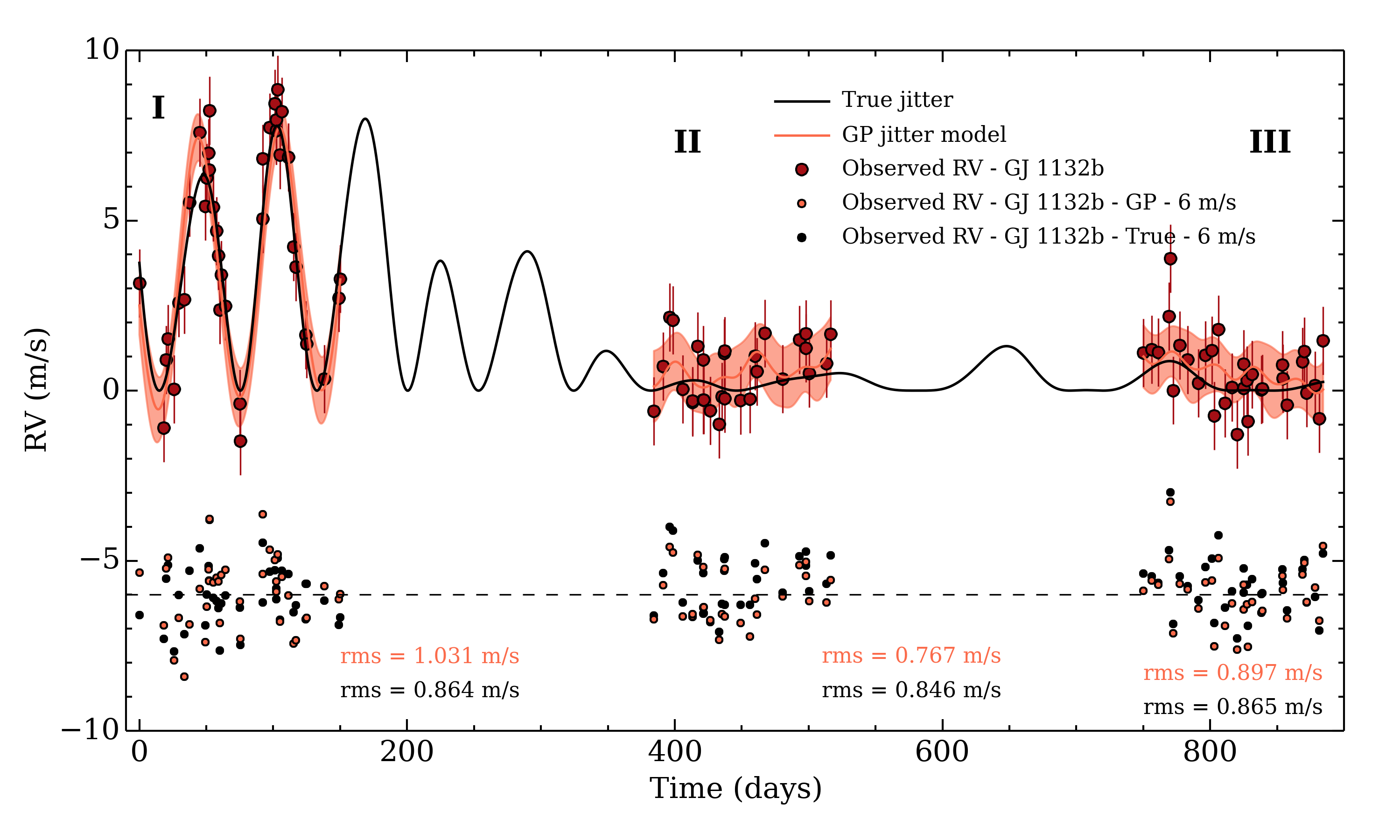
Figure 2.— An example of a 1-planet simulated RV timeseries on an arbitrary time axis and the keplarian contribution (from GJ 1132b) removed. The RV measurements (red circles) therefore contain stellar jitter, predominantly from the suppression of convective blueshift, and noise. The true jitter from which the data are derived is shown in black. The optimized quasi-periodic GP jitter model and 95% confidence intervals for each observing window (I,II,III) are shown in pink. The residuals about the true jitter are plotted as black points while the residuals about the GP jitter model are plotted as pink points. Both sets of residuals are shifted downwards by 6 m s^-1 for clarity. The rms of each set of residuals is annotated in the panel (residuals about the true jitter and GP jitter model in black and pink respectively).

In Fig. 2 we distinguish adjacent observing seasons by labelling them I, II, and III respectively. This is necessary because the GP jitter model behaves differently depending on the amplitude of the RV variation compared to the measurement uncertainties ($\sigma_{\mathrm{RV}}=1$ m s^-1 in Fig. 2) and the jitter amplitude itself varies between the three seasons. Fig. 1 revealed a long decaying timescale of the fractional coverage by active regions implying that the RV jitter will vary between stellar rotation cycles. In regions where the RV measurement amplitude is small (labelled II and III), the measurement dispersion is comparable to the underlying true jitter (black line) which causes the GP jitter model (pink line) to (incorrectly) find high-frequency structure that is not present in the true jitter; GP over-fitting. However, because the amplitude of the best-fit GP jitter model is comparable to the true jitter, the measurement residuals about the GP jitter model (pink dots) and the true jitter (black points) are consistent and on the order of $\sigma_{\mathrm{RV}}$ ($\sim 0.9$ m s^-1).

When the star is largely covered in active regions (labelled I), the jitter amplitude is $>\sigma_{\mathrm{RV}}$ and a GP is useful for modelling the jitter. In this case the residual rms about the GP jitter model is reduced to the level of $\sim 1$ m s^-1 and crucially, comparable to the residual rms of the observed RVs about the true jitter in the ‘quiet’ regions. Therefore we confirm that the use of a GP in modelling the jitter is an effective method of mitigating the jitter down to the level of the RV measurement uncertainties. In Sect. 5.2 we elaborate on the power of GP jitter models applied to rapid rotators where the jitter amplitude is significantly larger than it is for the slowly rotating GJ 1132.

3.2. Radial Velocity Timeseries Construction

3.2.1 Radial velocity contributions

In order to simulate a suite of planetary systems that could potentially exist in the GJ 1132 system, we construct a sample of hypothetical planetary systems and simulate their RV signals with jitter included. We refer to these components as the astrophysical terms in the timeseries. The astrophysical terms therefore include the keplarian signal from GJ 1132b, the aforementioned additional keplarian signals from hypothetical planets (see Sect. 3.3 for a description of these planets), and the stellar RV jitter due to rotating active regions derived in Sect. 3.1. Each astrophysical term is assumed to be independent.

In addition to these astrophysical sources, we add a noise model containing a white noise term with a fixed variance of 1 m s^-1 and a systematic noise term which permits us to vary the global noise properties of each timeseries in a simple, parameterized way. In practice, the total non-astrophysical noise injected into each timeseries varies from $\sigma_{\mathrm{RV}}\in[1,2]$ m s^-1. Given the late spectral type of GJ 1132b, a RV precision of 1 m s^-1 should be achievable (Figueira et al., 2016). The variance in the Gaussian noise term is chosen to resemble the long-term stability limit of current state-of-the-art velocimeters (e.g. HARPS; Mayor et al., 2003) which is also equal to the anticipated stability limit of some upcoming near-IR velocimeters (e.g. SPIRou; Delfosse et al. 2013; Artigau et al. 2014, Habitable Zone Planet Finder; Mahadevan et al. (2012), Infrared Doppler instrument; Kotani et al. (2014), CARMENES; Quirrenbach et al. 2014).

3.2.2 Time-sampling

For each simulated planetary system we observe the star N_obs times with N_obs $\in[40,300]$. The adopted limits on N_obs are motivated by the approximate number of RV measurements required to detect a planet in a blind survey and an assumed upper limit on a reasonable number of RV measurements per star respectively. A modest limit on the maximum value of N_obs also limits the computational cost of our study. The observations are taken at most twice per night over the course of 3 years, similar to the time baseline of a dedicated exoplanet RV survey. The observation timestamps are randomly drawn from the window function (time sampling) generated from the ephemeris of GJ 1132. Although the window function is based on the location of the HARPS-South instrument at La Silla Observatory in Chile, we exclude observation epochs during dark-time due to the priority reserved for imaging instruments during that time. Although this restriction does not affect the La Silla site, it will be applicable to instruments such as SPIRou at CFHT. From preliminary tests which relaxed the exclusion of dark-time epochs, this restriction was found to not have a significant effect on our results.

3.3. Planet Sample

In order to investigate the potential detection of additional planets around GJ 1132, we construct a sample of small planets according to the occurrence rates from the primary Kepler mission (Dressing & Charbonneau, 2015). We opt to use the planet occurrence rates derived from the Kepler transit survey, coupled to a planetary mass-radius relationship, rather than the occurrence rates derived from radial velocity surveys (e.g. Bonfils et al., 2013). This selection owes itself to the improved statistics resulting from the larger sample of transiting planets than radial velocity planets around M-dwarfs.

We find that dynamical stability arguments require that the planetary orbital periods $P$ of our simulated planets always be greater than that of GJ 1132b. Adopting the grid of planet radii $r_{p}$ and orbital periods from Dressing & Charbonneau (2015) restricts our analysis to $r_{p}\in[0.5,4]$ R_⊕ and $P\in(P_{\mathrm{b}},200]$ days where the subscript $b$ refers to GJ 1132b. To derive the expected RV signal from each simulated planet we convert $r_{p}$ to planet mass $m_{p}$ by simply assuming an Earth-like bulk density for planets with $r_{p}\leq 1.6$ R_⊕. The highest precision exoplanet mass and radius measurements ($\leq 20$% uncertainty) have shown that the upper limit on $r_{p}$ for rocky worlds (little-to-no volatiles) is $\sim 1.6$ R_⊕, below which most exoplanets have an Earth-like bulk density ($\sim 17$% Fe and 83% MgSiO₃ mass fraction; Zeng & Sasselov, 2013; Charbonneau, 2015; Dressing et al., 2015). This boundary has also been approximately confirmed from theoretical studies (e.g. Lopez & Fortney, 2014). The subset of planets with $r_{p}>1.6$ R_⊕ are assigned the bulk density of Neptune; a solid core surrounded by a gaseous envelop rich in volatiles. We refer to these two classes of planets as Earth-like ($\bar{\rho}=5.51$ g cm^-3) and Neptune-like ($\bar{\rho}=1.64$ g cm^-3) compositions respectively. Adopting this mass-radius relationship represents a conservative choice in the sense that if instead we adopt a probabilistic mass-radius relationship motivated by the empirical distribution of exoplanetary masses and radii, such as that from Weiss & Marcy (2014), the resulting planetary masses are often found to be greater than those which are obtained when assuming either an Earth-like or Neptune-like bulk density. Therefore, for a fixed $r_{p}$ the planet is more easily detectable assuming the mass-radius relationship from Weiss & Marcy (2014) thus making the adopted mass-radius relationship a conservative choice. The implications of changing the mass-radius relationship are discussed in detail in Sect. 5.4.

3.3.1 Dynamical considerations

At the orbital periods considered, the circularization timescale of simulated planets need not be less than the assumed age of the system ($\sim 5$ Gyrs; B15). Therefore we do not fix simulated planets on circular orbits and instead randomly draw orbital eccentricities from the Beta distribution in Cloutier et al. (2015) used to describe the eccentricity distribution of RV exoplanets detected with high significance (Kipping, 2013). Assuming planets around GJ 1132 are remnant bodies from a primordial debris disk that is collisionally relaxed following the planet formation process (Raymond et al., 2005; Kokubo et al., 2006), the eccentricity dispersion within any planetary system $\langle e^{2}\rangle$ is related to the dispersion in orbital inclinations via $\langle i^{2}\rangle\sim\langle e^{2}\rangle/4$ radians (Stewart & Ida, 2000; Quillen et al., 2007) which we use to sample the mutual inclinations of drawn planets. Furthermore, because small exoplanets around M-dwarfs in multiple systems have been shown to have lower eccentricities than their giant planet counterparts (Kane et al., 2012; Van Eylen & Albrecht, 2015), we focus on orbital eccentricities $\lesssim 0.5$. This also ensures that the inclinations of simulated planetary systems resemble the empirical distribution containing mostly low mutually inclined compact systems (Figueira et al., 2012; Fabrycky et al., 2014).

Because in our test case we are interested in detecting additional planets in a planetary system with one confirmed planet, dynamical stability arguments further restrict the types of multi-planet systems that can potentially be present around GJ 1132. We therefore impose additional, analytical constraints on simulated planetary systems in an attempt to ensure that simulated planetary systems are dynamically stable without having to perform detailed N-body simulations of every simulated system. Specifically, we constrain the simulated planet eccentricities to ensure that the orbits of GJ 1132b and the added planets do not cross. We also insist that each planetary system be Lagrange stable which naturally implies Hill stability (Marchal & Bozis, 1982; Duncan et al., 1989; Gladman, 1993). Lagrange stability requires that the ordering of planets remains fixed, that both planets remain bound to the central star, and also places limits on permissible changes in planets’ semimajor axes and eccentricities making the Lagrange stability criterion a more stringent definition of stability than Hill stability alone. The approximate condition for Lagrange stability is $\delta\gtrsim 1.1\delta_{\mathrm{crit}}$ (Barnes & Greenberg, 2006) where $\delta=\sqrt{a_{\mathrm{out}}/a_{\mathrm{in}}}$ and $\delta_{\mathrm{crit}}$ is the value of $\delta$ which satisfies

$$\alpha^{-3}(\mu_{1}+\frac{\mu_{2}}{\delta_{\mathrm{crit}}^{2}})(\mu_{1}\gamma_{1}+\mu_{2}\gamma_{2}\delta_{\mathrm{crit}}^{2})=1+\mu_{1}\mu_{2}\left(\frac{3}{\alpha}\right)^{4/3},$$ (1)

where $\mu_{i}=m_{p,i}/M_{s}$, $\alpha=\mu_{1}+\mu_{2}$, and $\gamma_{i}=\sqrt{1-e_{i}^{2}}$ (Gladman, 1993). The Lagrange stability criterion is therefore uniquely determined by the system body masses, orbital separations, and eccentricities. Strictly speaking, the analytical Lagrange stability criterion is only applicable to three-body systems (star + two planets). We therefore apply the stability criterion to adjacent pairs of planets in systems with multiplicity $>2$ noting however that such systems may include significant planet-planet interactions whose effects on system stability are not captured by the analytic Lagrange stability criterion.

As there is no analytical stability criterion for systems with multiplicity $>2$, we supplement the Lagrange stability criterion with the heuristic stability criterion from Fabrycky et al. (2012) which is derived from suites of numerical integrations of high multiplicity systems (Smith & Lissauer, 2009). Fabrycky et al. (2012) reported that a system with $\Delta_{\mathrm{in}}+\Delta_{\mathrm{out}}>18$ will be dynamically stable where $\Delta=(a_{\mathrm{out}}-a_{\mathrm{in}})/R_{\mathrm{Hill}}$, the subscripts ‘in’ and ‘out’ refer to the inner and outer planet respectively, and $R_{\mathrm{Hill}}$ is the mutual Hill radius of adjacent planet pairs. Applying these conditions to the ensemble of simulated planetary systems results in a planet sample that is weakly biased away from short-period, massive planets. The resulting planet distribution is therefore not equivalent to the initial planet distribution of Dressing & Charbonneau (2015).

All together, these limiting conditions help to ensure that additional planets around GJ 1132 do not invoke a strong gravitational interaction on GJ 1132b. This is motivated by the fact that the GJ 1132b transit light curves do not exhibit any significant transit timing or transit duration variations (B15). This constraint greatly simplifies the analysis as it implies that the total RV signal resulting from multiple planetary companions can be sufficiently described by the superposition of keplarian orbits rather than a computationally expensive, fully dynamical model. To facilitate this methodology of constructing synthetic RV timeseries via multiple keplarian orbits we also demand that planet pairs not exist close to any low-order mean-motion resonance wherein the keplarian approximation would break down as evidenced by the large associated transit-timing variation amplitudes in low mutually inclined systems (Agol et al., 2005; Payne et al., 2010).

3.3.2 Planet sample at a glance

The full distributions of simulated planet orbital periods and masses are shown in Fig. 3. Orbital periods are shown in various planet radius bins and are compared to the Dressing & Charbonneau (2015) distribution from which they were initially drawn. Unsurprisingly, our sample is consistent with that of Dressing & Charbonneau (2015) within reported uncertainties for periods $\gtrsim 5$ days. For massive planets ($r_{p}\geq 3$ R_⊕) with orbital periods below this limit but still $>P_{b}$, issues regarding dynamical stability between the simulated planet and GJ 1132b begin to limit the planet sample there. The same stability argument results in no simulated planets with orbital periods $<P_{b}$ in the GJ 1132 system despite there non-zero occurrence rate.

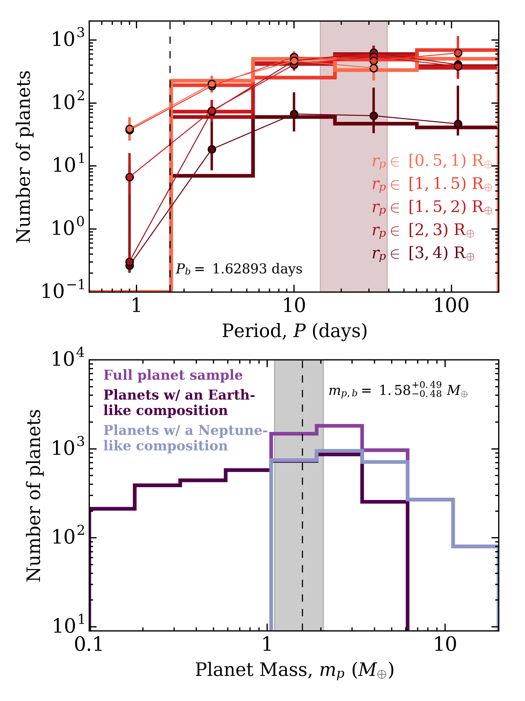
Figure 3.— Distributions of simulated planet properties. Top: orbital periods in various planet radius bins. The circular markers represent the scaled period distribution from Dressing & Charbonneau (2015) in identical radius bins. The vertical dashed line depicts the orbital period of GJ 1132b. The shaded region highlights the adopted definition of the star’s habitable zone (see Sect. 4.3; $14.7-39.2$ days) Bottom: the full sample of planet masses along with the sub-samples of rocky and gaseous planets. The vertical dashed line and shaded region depicts the MAP value and $1\sigma$ uncertainty of the GJ 1132b planet mass from our Gaussian process + keplarian fit. (Sect. 3.4).

Based on the adopted mass-radius relation, the distribution of planet masses in the simulation is split roughly evenly between rocky and volatile-rich planetary compositions with a slight excess of rocky planets ($\sim 55$% rocky). Furthermore, the distribution of simulated planet masses has a median value of $\sim 1.9$ M_⊕ and the subset of the most massive planets ($m_{p}\gtrsim 4$ M_⊕), hence the most easily detectable with radial velocities, are not expected to have a rocky bulk composition.

3.4. Planet Detection

In order to detect additional planets around GJ 1132 in the synthetic RV timeseries in our MC simulations, we compute the Bayesian model evidences for models with an increasing number of keplarian orbital solutions (i.e. no planets, 1 planet, and 2 planets). From these values we can determine the optimal number of planets supported by each dataset and thus the number of detected planets. This method is commonly used to detect planetary signals in RV timeseries (e.g. Ford & Gregory, 2007; Feroz & Hobson, 2014).

We reserve a more complete description of the adopted Bayesian model selection formalism for appendix B. To summarize, the Bayesian model evidence $Z_{k}$ (Eq. B5) for each independent model $M_{k}$ where $k=0,1,2$ is the number of keplarian solutions in the model, is computed using the Multinest (Feroz & Hobson, 2008; Feroz et al., 2009; Feroz & Hobson, 2014) nested sampling algorithm to sample from the unique model parameter posteriors and efficiently calculate the model evidences from a specified logarithmic likelihood function (Eq. B6) and appropriately chosen model parameter priors.

For the single planet model $M_{1}$, the set of model parameters $(P,T0,K)$ corresponds to the measured values for GJ 1132b and are therefore well constrained by the transit light curves and RV measurements from B15. For each parameter we adopt a uniform prior within the parameter’s $1\sigma$ uncertainty from Table 1.

The case is somewhat more complicated for the 2-planet model. Because the expense of calculating the evidence integral in Eq. B5 grows rapidly with the dimensionality of the model and the domain of the model parameter space, we restrict the analysis to a subset of parameter values obtained from the results of a Lomb-Scargle periodogram (Scargle, 1982; Gilliland & Baliunas, 1987) analysis of the residual RV dataset following the removal of the GJ 1132b keplarian signal. Namely, we construct a broad uniform prior on $P_{c}$ (we label the second planet in the $M_{2}$ model with the subscript $c$) centered on the most significant periodogram peak $P_{\mathrm{peak}}$ with a false-alarm probability (FAP) $\leq 0.01$. Each peak’s FAP is computed using the analytical approximation of (Baluev, 2008; Meschiari et al., 2009). The analytical estimation for small FAPs (FAP $\lesssim 0.001$) is known to be inaccurate (Cumming, 2004) so instead we settle for an upper bound on the FAP which is still indicative of a period ‘detection’. Limits on the period prior are placed at $\pm 5$% which is intended to span the peak value without being too restrictive as the location of the peak in the discrete periodogram need not correspond exactly to the period of the input planet. Furthermore, we avoid peaks located within 2% of the stellar rotation period or its low-order harmonics (i.e. 122.31, 61.15, 40.77, 30.58 days). We then adopt broad uniform priors of $T0_{c}\in[T0_{b}-P_{\mathrm{peak}}/2,T0_{b}+P_{\mathrm{peak}}/2]$ BJD and $K_{c}\in(0,15]$ m s^-1. In this way, the detection of additional planets around GJ 1132 requires a small false-alarm probability peak in the Lomb-Scargle periodogram of the timeseries as well as favorable evidence for the two planet model.

From the calculated model evidences we compute the Bayes factor, or the ratio of evidences $R_{mn}=Z_{m}/Z_{n}$ (see also Eq. B2), for arbitrary models $m,n=0,1,2$. Using the interpretation scheme outlined in Kass & Raftery (1995), we claim that a hypothetical second planet, not detected in transit, is marginally detected in a RV dataset if $R_{21}>3$ and is a bona fide detection if $R_{21}>20$.

3.4.1 Planet detection in the published radial velocities of GJ 1132

As a check, we apply our planet detection method to the 25 published RV measurements from B15 using a GP, trained on the MEarth photometry, to model the correlated components in the RV data arising from stellar rotation. The resulting semiamplitude and planet mass of GJ 1132b are consistent with the results from (B15) implying that use of a GP noise model does not have a significant effect on the recovery of planet parameters for this particular system. This is unsurprising given that the RV data were obtained over only $\sim 1/3$ of a rotation cycle and the errorbars on those measurements were comparable to the expected RV jitter from active regions (Sect. 3.1.2). The maximum a posteriori (MAP) values of $K_{b}$ and $m_{p,b}$ from this analysis are reported in Table 1.

As an additional check, this analysis also confirmed that a single planet RV model is strongly favored over the null hypothesis using the aforementioned priors on the orbital period and time of mid-transit from the transit lightcurves (B15) to reduce the computation time, but expanding the prior on $K_{b}$ to $\in(0,15]$ m s^-1. The single planet model also shows positive evidence compared to a 2-planet model indicating that a ‘GJ 1132c’ is not detected in the dataset. This highlights the fact that the eventual detection of additional planets in the GJ 1132 system will require extensive RV follow-up observations. The complete model evidences based on the published RV data are given in Table 2.

Table 2Model evidences $Z$ based on the published GJ 1132 radial velocity timeseries

Model	$\ln{Z}$	Bayes factor	Interpretation
No planets ($M_{0}$)	$-48.06\pm 0.01$	-	-
One planet ($M_{1}$; GJ 1132b)	$-45.05\pm 0.02$	$R_{10}=20.31\pm 1.01$	The single planet model is strongly
			favoured over the null hypothesis.
Two planets ($M_{2}$)	$-46.48\pm 0.03$	$R_{12}=4.16\pm 0.99$	The single planet model is positively
			favoured over the two planet model.

4. Results

The detection completeness to additional planets in the known transiting system is computed using $10^{3}$ realizations of our MC simulation for each of the three values of the RV measurement uncertainty $\sigma_{\mathrm{RV}}=1,1.5,2$ m s^-1, which are calculated by the quadrature sum of parameterized white and systematic noise sources. Uncertainties on the computed detection completeness are calculated using Poisson statistics. We find that planetary systems with the minimum multiplicity of one never find strong evidence for an additional planet. These systems are included in the completeness calculation because the null detection of a non-existent planet should not decrease the detection completeness. For systems with multiplicity $>2$, we only focus on detecting one of the simulated planets. The planet assigned to be the ‘target’ planet is simply the planet with the largest semiamplitude and will therefore have the most significant contribution to a periodogram of the timeseries. We do not attempt to detect more than two planets given the large size of the planetary system sample and the increased computation required to compute model evidences in systems with multiplicity $>2$.

4.1. Full Planet Detection Completeness

The detection completeness of our full MC planet sample is shown in Fig. 4. Initially, the detection completeness curves increase rapidly with the initial slope of the curve decreasing with $\sigma_{\mathrm{RV}}$ implying that as the noise properties improve, one achieves a favorable detection completeness with fewer RV measurements. The detection completeness curves asymptotically approach maximum values which tend to increase with $\sigma_{\mathrm{RV}}$ as expected.

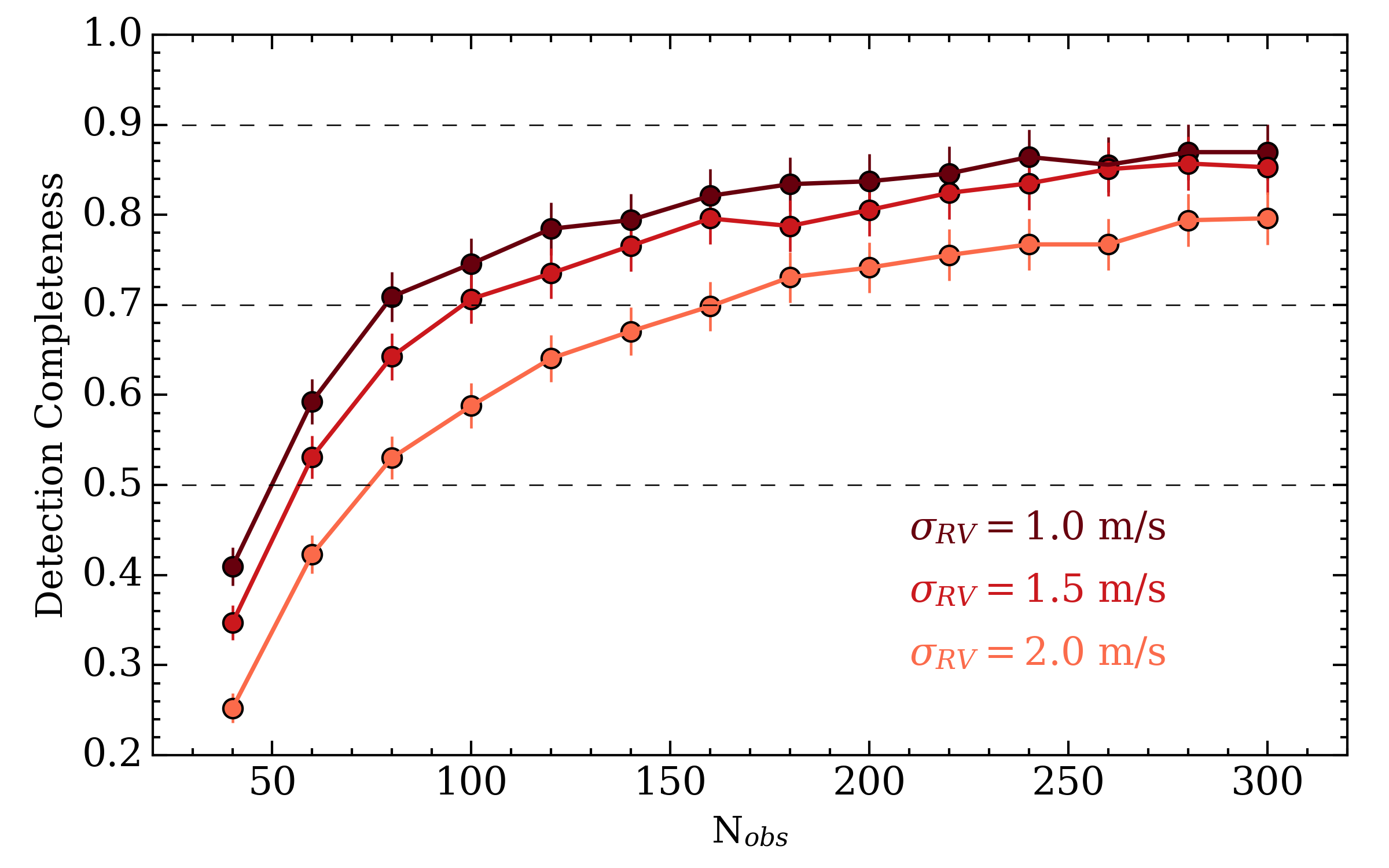
Figure 4.— The detection completeness for the entire sample ($r_{p}\in[0.5,4]$ R_⊕ and $P\in(P_{\mathrm{b}},200]$ days) of simulated planets not seen in transit around GJ 1132 for various values of the RV measurement uncertainty. Errorbars are from Poisson statistics. Dashed horizontal lines at 50, 70, and 90 per cent completeness are included to guide the eye.

In the best case scenario where the RV measurement uncertainty is equal to the long-term instrument stability limit of $\sigma_{\mathrm{RV}}=1$ m s^-1, we are sensitive to $\geq 50$% of all additional planets even with as little as 50 RV measurements. In this case the maximum detection completeness of $\sim 85$% is achieved for N_obs $\geq 200$.

Similarly, for the largest considered RV measurement uncertainty of $\sigma_{\mathrm{RV}}=2$ m s^-1, the detection completeness reaches $\sim 50$% by N_obs $\sim 75$ and continues to a maximum of 80% which is $\sim 7$% less than what is achieved with $\sigma_{\mathrm{RV}}=1$ m s^-1. In general, one loses just $\sim 7-15$% of detections across all N_obs with an increase in $\sigma_{\mathrm{RV}}$ from 1 to 2 m s^-1. Depending on the goals of an observer regarding their desired detection completeness, the detriment exhibited by increasing $\sigma_{\mathrm{RV}}$ to 2 m s^-1 may not be so harmful to the results. Furthermore, assuming that observational uncertainties are dominated by shot noise, settling for $\sigma_{\mathrm{RV}}=2$ m s^-1 only requires $\sim 1/4$ of the integration time as for $\sigma_{\mathrm{RV}}=1$ m s^-1 (Bouchy et al., 2001) thus allowing for a deeper planet detection completeness to be achieved with the same amount of telescope time.

4.2. Detection Completeness in Semiamplitude Bins

Here we bin our planet sample into four semiamplitude bins each containing roughly the same fraction of the full planetary sample ($20-30$% per bin). The resulting detection completeness for each value of $\sigma_{\mathrm{RV}}$ is shown in Fig. 5. Note that the Poisson errors on the curves are larger than in Fig. 4 as a result of the binning.

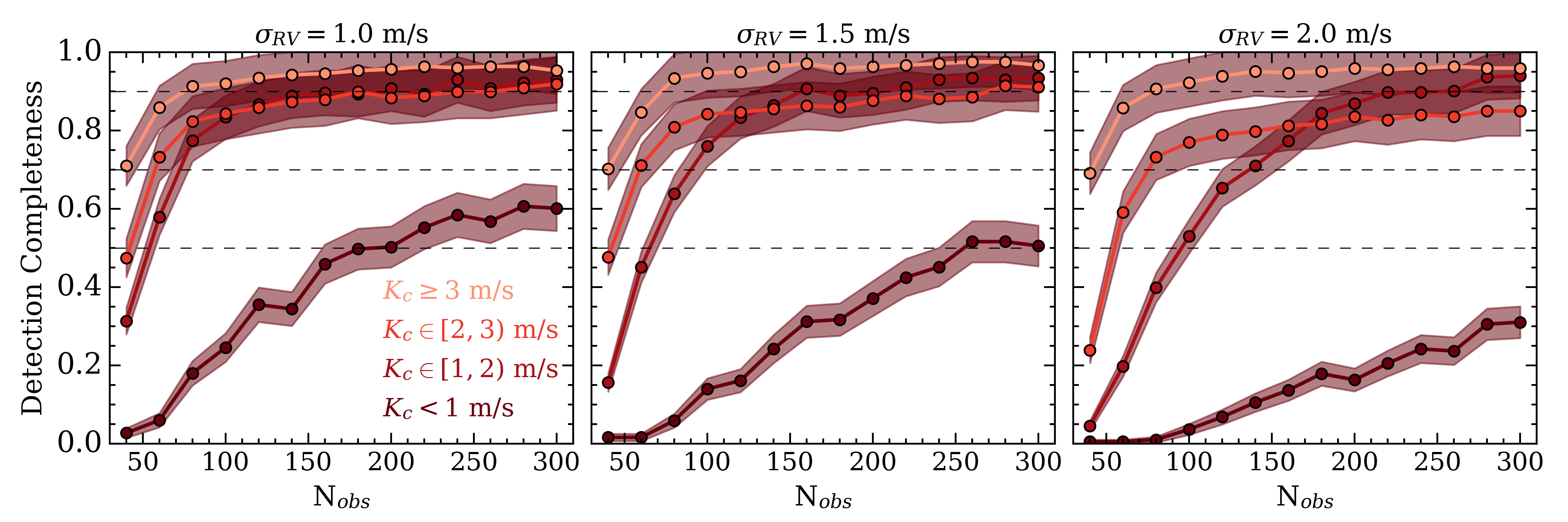
Figure 5.— Same as Fig. 4 but for planets in various RV semiamplitude bins. Each panel reports the completeness for a sample with the RV measurement uncertainty annotated above the panel. The shaded regions depict the errors from Poisson statistics. Dashed horizontal lines at 50, 70, and 90 per cent completeness are included to guide the eye.

Planets with $K_{c}<1$ m s^-1 have signals below the minimum RV measurement uncertainty and are hence difficult to detect though not impossible. In the cases of $\sigma_{\mathrm{RV}}<2$ m s^-1, we can achieve $>50$% detection completeness with N_obs $<300$. Planets with $K_{c}\geq 1$ m s^-1 represent the planets which are nominally detectable with current instrumentation and contribute the most to the detect completeness curves presented in Fig. 4. As expected, the planet detection completeness to planets with larger RV signals increases in general. However, when the level of RV measurement uncertainty becomes comparable to the mean semiamplitude of a bin in Fig. 5 (second and third panels), there can be some confusion in the completeness curves wherein planets with smaller $K$ appear to have improved detection statistics. We note however that these confused curves are still consistent within their Poisson errors.

From the completeness curves presented in Fig. 5, we claim that it is not an unreasonable observational task to detect $\gtrsim 80$% (50%) of planets in a system like GJ 1132 with $K_{c}\geq 1$ m s^-1 for $\sigma_{\mathrm{RV}}=1$ (2) m s^-1.

4.3. Detection Completeness of Potentially Habitable Planets

The habitable zone (HZ) around a given star refers to the orbital separations at which liquid water can exist on a planet’s surface (Dole, 1964; Hart, 1979). Yet, given that simple definition the boundaries of the HZ have not been unambiguously well-defined. This is understandable given the multitude of parameters that can affect the planetary surface conditions. Among these effects are the atmospheric mass and composition which can alter the planetary surface pressure and thus the relevant temperatures for phases changes of water (Vladilo et al., 2013). The presence of clouds can also have profound effects on the heating and cooling of the planet and therefore alter the orbital separations of the HZ (Selsis et al., 2007; Yang et al., 2013). Certain geometries of the system, including planet obliquity (Williams & Kasting, 1997; Spiegel et al., 2008, 2009) and orbital eccentricity (Dressing et al., 2010; Cowan et al., 2012), may also have an effect on the long term habitability of a planet.

For this study, we adopt a conservative definition of the HZ based on the parametric model of Kopparapu et al. (2013) which is derived using a 1D radiative-convective climate model in the absence of clouds. Following Kasting et al. (1993), the inner edge of the HZ is defined by the ‘water-loss’ or moist greenhouse limit wherein an increase in insolation would result in the photolysis of water in the upper atmosphere and result in subsequent hydrogen escape. We note that the inclusion of clouds may decrease the HZ inner edge as a result of the reflective properties of clouds. The outer edge of the HZ is determined by the maximum greenhouse limit wherein an increase in atmospheric CO₂ levels results in a net cooling as the effect of the increased albedo from Rayleigh scattering dominates over the additional greenhouse effect. We performed a small suite of tests using alternative parameterizations of the inner HZ edge from Yang et al. (2014) (for a cloudy, slowly rotating planet. These tests concluded that our completeness results are not strongly affected by the various assumptions regarding the HZ.

Assuming for GJ 1132 the stellar effective temperature and luminosity from Table 1, the resulting inner and outer HZ limits are 14.7 and 39.2 days respectively. We compile the set of potentially habitable planets by isolating the subset of planets which are rocky and whose orbital periods lie within the aforementioned HZ bounds. The detection completeness for this sub-sample is shown in Fig. 6 for various values of $\sigma_{\mathrm{RV}}$. For comparison we also include the completeness limits for rocky planets (Earth-like composition) and planets with extended envelopes (Neptune-like composition).

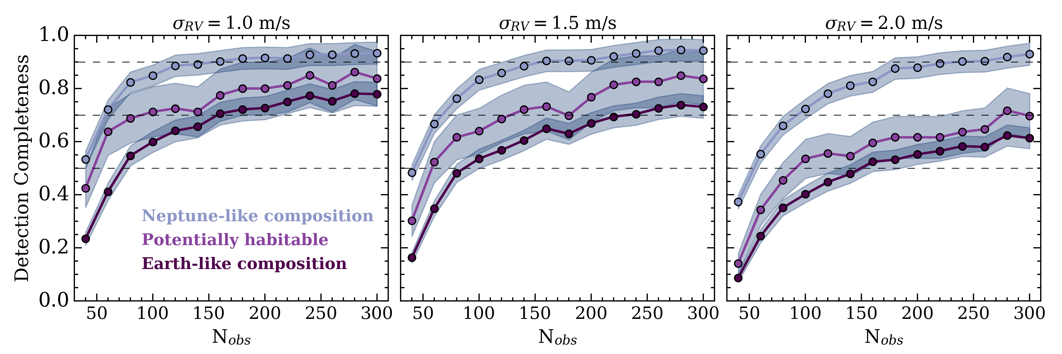
Figure 6.— Same as Fig. 4 but for the subset of planets that i) have volatile-rich envelops (Neptune-like composition), ii) are rocky (Earth-like composition), and iii) are both rocky and lie within the habitable zone of GJ 1132. Each panel reports the completeness for a sample with the RV measurement uncertainty annotated above the panel. The shaded regions depict the errors from Poisson statistics. Dashed horizontal lines at 50, 70, and 90 per cent completeness are included to guide the eye.

In the best case scenario where $\sigma_{\mathrm{RV}}=1$ m s^-1, we are 50% complete for detecting potentially habitable planets with N_obs $\sim 50$. A maximum detection completeness of $\sim 85$% is then realized at N_obs $\sim 200$ although it is difficult to place an exact boundary on where the maximum completeness is reached given the comparatively large Poisson errors on the potentially habitable planet completeness curve. If $\sigma_{\mathrm{RV}}$ is doubled, the maximum detection completeness falls to $\sim 70$%. These complete curves for potentially habitable planets are very similar to the equivalent curves for the full sample of planets (c.f. Fig. 4). We therefore conclude that we are as efficient at detecting potentially habitable planets as we are to detecting all planets.

Comparing the potentially habitable completeness curves to the detection completeness of all rocky planets in the sample, we observe that we are more sensitive to HZ rocky planets than to the total population of rocky planets. Fig. 7 reveals that the period range over which we are maximally efficient at detecting planets approximately corresponds to the inner edge of the habitable zone. At both shorter and longer orbital periods, the detection completeness falls significantly compared to the domain of maximum completeness approximately spanning $P\in[5,20]$ days, which spans the inner HZ edge. Recall that we have intentionally avoided periodicities close to the stellar rotation period and its low-order harmonics including $P_{\mathrm{rot}}/2$; the effective periodicity of the RV jitter from the $FF^{\prime}$ method. We draw attention to these periods because the detection completeness of planets with orbital periods close to these periodicities is artificially reduced. However, the fraction of planets within only $\pm 2$% of either $P_{\mathrm{rot}}$ or $P_{\mathrm{rot}}/2$ is small such that the maximum detection efficiency still corresponds to the peak in Fig. 7.

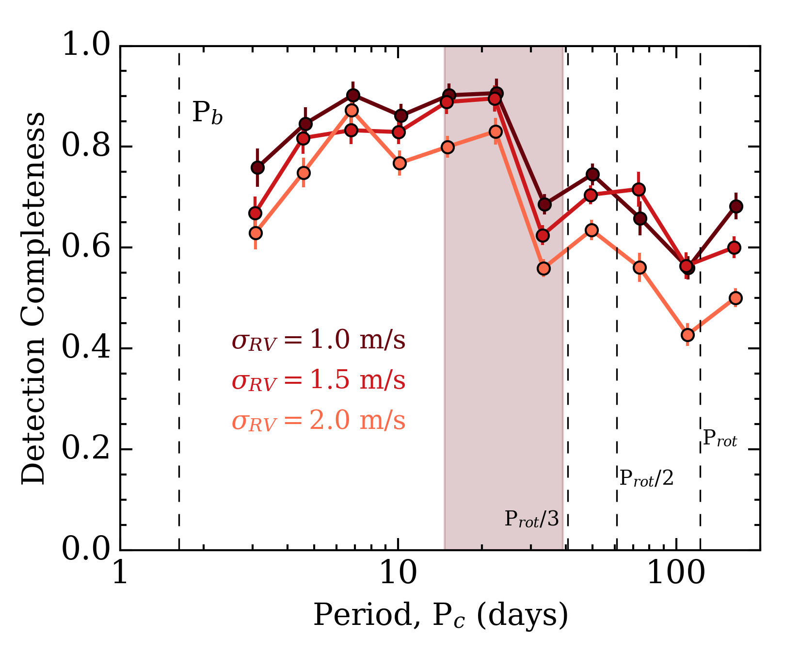
Figure 7.— Detection completeness as a function of orbital period and RV measurement uncertainty. The vertical dashed lines highlight the orbital period of GJ 1132b ($P_{b}=1.62893$ days), the stellar rotation period ($P_{\mathrm{rot}}=122.31$ days), and its harmonics. The habitable zone is depicted in the shaded red region.

Returning to Fig. 6 we also note that, unsurprisingly, we are far more sensitive to large ($r_{p,c}>1.6$ R_⊕), Neptune-like planets given their corresponding large masses compared to the Earth-like planets in the sample (c.f. Fig. 3). Regardless of $\sigma_{\mathrm{RV}}$, the detection of Neptune-like planets is always at least 20% more complete than for Earth-like planets for all values of N_obs.

4.4. Period-Mass Plane

To aid in the interpretation of the results from our MC simulations we plot the distribution of simulated planets in the period-mass plane in Fig. 8 and indicate which planets are detected with N_obs $\leq 100$. We do this for the case of zero systematic uncertainty; $\sigma_{\mathrm{RV}}=1$ m s^-1. For reference, the detection completeness for this full sample and the subset of potentially habitable planets is $75\pm 3$% and $71\pm 9$% respectively.

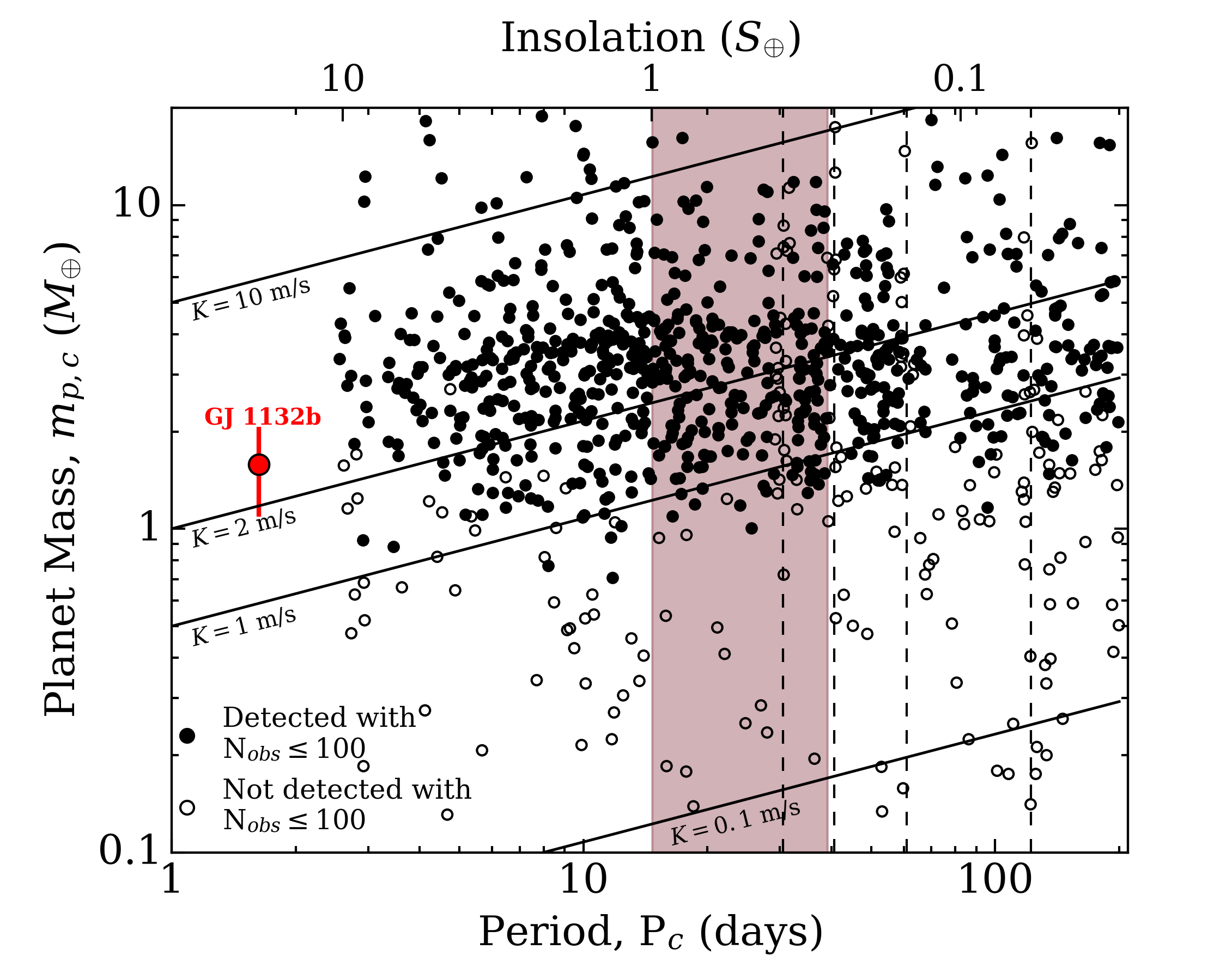
Figure 8.— The planetary mass-period/insolation plane of our full MC planet sample with $\sigma_{\mathrm{RV}}=1$ m s^-1. Planets which are detected with $\leq 100$ RV measurements are shown in black whereas planets which remain undetected are shown in white. Contours of constant RV semiamplitude are over-plotted as sold black lines. The vertical dashed lines indicate the rotation period of GJ 1132 and its low-order harmonics. The habitable zone is depicted in the shaded red region. GJ 1132b is highlight as the red circle.

Notable features include the significant fraction of planets detected with $K_{c}\geq 1$ m s^-1 including a population of sub m s^-1 planets with orbital periods $\gtrsim 10$ days. There is also a distinct dearth of planets with $P_{c}\lesssim 2.5$ days. This is a consequence of the existence of GJ 1132b with $P_{b}=1.62893$ days and the dynamical stability arguments imposed on each simulated planetary system.

Also recall that we purposely ignore periodicities in the Lomb-Scargle periodogram analysis which lie close to the stellar rotation period and its low-order harmonics. Such planets lie close to the vertical dashed lines in Fig. 8 but appear to be embedded in regions where their nearest neighbours are detected. Therefore, if the stellar rotation period were to vary slightly from $P_{\mathrm{rot}}=122$ days, then these planets would likely be detected potentially increasing the detection completeness. Some of these disregarded planets also appear to lie within the habitable zone, making our detection completeness of potentially habitable planets around GJ 1132 more favorable.

5. Discussion

5.1. Applicability to Other Systems

Our work regarding the effort required to recover additional planets around slowly rotating M-dwarfs such as GJ 1132 is applicable to other systems containing at least one transiting planet such as those which will be discovered with TESS (Ricker et al., 2014; Sullivan et al., 2015). The condition of slow rotation is required to focus on systems with similarly low noise statistics from stellar jitter (see Sect. 3.1).

Numerous studies of the rotation period distribution of M-dwarfs ($T_{\mathrm{eff}}\leq 3800$ K) have concluded that two populations exist corresponding to fast and slow rotators (e.g. Irwin et al., 2011; McQuillan et al., 2013a, 2014; Newton et al., 2016b). This dichotomy among M-dwarfs is posited to arise from magnetic braking; angular momentum loss by strongly magnetized stellar winds (Reiners & Mohanty, 2012). This implies that the rotation period of these low-mass, convective stars might be used to infer stellar ages via gyrochronology (Barnes, 2003, 2007). Indeed the empirical distribution of M-dwarf rotation periods is in good agreement with the inferred distribution derived from gyrochronology (McQuillan et al., 2014). By this logic, GJ 1132 is an old ($\sim 5$ Gyrs) star which belongs to a large population of slowly rotating ($P_{\mathrm{rot}}\gtrsim 40$ days; Newton et al., 2016b) M-dwarfs with correspondingly low RV jitter levels of just a few m s^-1 or comparable to the demonstrated and anticipated stability limit of state-of-the-art velocimeters.

From the rotation period distribution of Newton et al. (2016b), roughly 40% of TESS M-dwarfs with planet candidates are expected to exhibit slow rotation and correspondingly low RV jitter levels similar to GJ 1132. For these systems, which will require RV follow-up observations to characterize planet masses and search for additional non-transiting planets, their orbital periods will be well-characterized by the transit observations thus allowing the detection completeness to additional small planets around the star to not differ significantly from what we have shown in this study. This is because the orbital period and time of mid-transit for the transiting planet candidates will be well-characterized by TESS implying that the keplarian signal of the candidate can be removed from a RV timeseries with relative ease once its mass and orbital elements have been adequately constrained (see Sect. 5.3). The search for additional planets then proceeds identically to the investigation presented in this paper.

Indeed the applicability of our detection completeness calculations is only true for slowly rotating M-dwarfs which are sufficiently bright such that a RV stability limit of $\sigma_{\mathrm{RV}}\lesssim 2$ m s^-1 can be achieved. For the upcoming near-IR spectropolarimeter SPIRou, $\sigma_{\mathrm{RV}}\sim 1$ m s^-1 is expected to be readily achieved for stars brighter than $\sim 9.5$ in the $J$ band. TESS is predicted to find $\sim 50$ such stars with transiting planets (Sullivan et al., 2015). Other current and upcoming near-IR spectrographs are anticipated to be able to achieve similar stability limits. Furthermore, from the full TESS survey predictions of Sullivan et al. (2015), and the empirical stellar rotation period distribution as a function of stellar mass, we expect our detection completeness curves (Figs. 4, 5, and 6) to be relevant to $\sim 300$ M-dwarfs from the TESS catalogue. Although, special considerations will be required to observe stars with $9.5\lesssim J\lesssim 11$ if $\sigma_{\mathrm{RV}}\lesssim 2$ m s^-1 is to be achieved. Optimistically, this number may even represent a lower limit given the apparent dearth of planets around rapidly rotating stars (McQuillan et al., 2013b) implying that the population of detected TESS candidates may preferentially exist around slow rotators.

However, a notable concern exists for potentially habitable planets around M-dwarfs wherein the orbital periods corresponding to the HZ may be close to the stellar rotation period and its low-order harmonics thus making it difficult to detect such planets (Vanderburg et al., 2016). With that in mind, Newton et al. (2016a) argued that M-dwarfs with spectral classes M4-M6 ($0.1\lesssim M_{s}/$M${}_{\odot}\lesssim 0.25$) represent the best possible candidates for finding HZ planets around cool stars as their HZ limits lie within the peaks of the M-dwarf rotation period distribution.

5.2. Detecting Planets Around Active Stars Using Gaussian Processes

As we have noted, this study is most applicable to cases of known transiting systems around M-dwarfs with rotation periods $\gtrsim 40$ days. These systems are enticing for the search for small planets because the rotationally-induced RV jitter is expected to be ‘manageable’. In Sect. 3.1.2 we showed that when the RV jitter amplitude is $>\sigma_{\mathrm{RV}}$, that a GP trained on the star’s light curve can effectively model the jitter and bring the rms of the residuals (RVs minus jitter model) to the level of $\sim\sigma_{\mathrm{RV}}$ (c.f. Fig. 2).

However there exists a substantial fraction of M-dwarfs which belong to either a kinematically young population or are among the latest M-dwarfs which can remain magnetically active even with $P_{\mathrm{rot}}>40$ days (West et al., 2015). In these cases, the search for planets may not proceed identically to the methodology of this study due to the large amplitude RV jitter. Following the work of a number of other authors (e.g. Haywood et al., 2014; Rajpaul et al., 2015) here we show how a Gaussian process, trained on an activity diagnostic timeseries, can still be used to model the jitter from active regions and detect planets with $K$ much less than the stellar RV jitter signal. Accurate jitter modelling in rapidly rotating M-dwarf systems also facilitates the detection of the Rossiter-McLaughlin effect from small planets thus providing a direct measure of the angular momentum evolution in such systems (Cloutier & Triaud, 2016).

In particular, we consider a case identical to the GJ 1132 planetary system ($P_{b}\sim 1.63$ days, $K_{b}=2.69$ m s^-1) but we decrease the stellar rotation period by more than an order of magnitude to $P_{\mathrm{rot}}=2$ days and correspondingly increase the amplitude of the star’s photometric variability to a more suitable value of $10^{4}$ parts per million (ppm; Newton et al., 2016b). In this case the consequential RV jitter amplitude is $\sim 60$ m s^-1 (Aigrain et al., 2012) instead of $\sim 8$ m s^-1. We construct a photometric timeseries from a simple sinusoid with the aforementioned period and amplitude, and a white-noise term with a typical dispersion of 1000 ppm (Newton et al., 2016b). We then derive the expected RV jitter timeseries from the light curve using the analytical prescription of Aigrain et al. (2012). A synthetic RV timeseries is then created via the sum of the stellar jitter, derived from the synthetic light curve, and the GJ 1132b keplarian signal. We assume a fixed RV uncertainty of $\sigma_{\mathrm{RV}}=1$ m s^-1 for this exercise.

To model the effect of active regions and attempt to remove it and search for any planetary signals in the residuals, the methodology identical to what was used in Sect. 3.1.2 is adopted. In summary, we train a quasi-periodic Gaussian process (GP) on the stellar light curve. The marginalized posterior probability distributions functions for the GP hyperparameters are derived using MCMC which are then used to compute a photometric model from which the RV jitter model is derived. This method of training the GP jitter model on an activity diagnostic timeseries and subsequently using the hyperparameter priors to model the observed RV with a GP + keplarian model has been successfully used on systems with jitter levels of a few to $\sim 10$ times greater than the planetary signal (Baluev, 2013; Haywood et al., 2014; Grunblatt et al., 2015), as is true in our current test case.

The best evidence for detecting the planet following the removal of our MAP jitter model comes from a Lomb-Scargle periodogram given that we know the injected planet’s orbital period. The upper panel of Fig. 9 shows the periodogram of the photometric timeseries with an unambiguous peak at the 2 day stellar rotation period (FAP $<0.1$%). This should be obvious given the imposed sinusoidal nature of the synthetic light curve. The middle panel then shows the periodogram of the raw RV timeseries (active regions+planet+noise) with a significant peak at the first harmonic of the stellar rotation period; $P_{\mathrm{rot}}/2$. We expect to see the strongest periodicity at $P_{\mathrm{rot}}/2$ if the RV variation is strongly affected by the flux effect (see Sect. 3.1.2) from active regions, as is the case for rapidly rotating stars, because this effect scales linearly with the first time derivative of the light curve. Because of the strong jitter signal compared to the planetary signal, the periodogram power at $P_{b}$ is well beneath the noise in this timeseries. Therefore we clearly do not detect the injected planetary signal when the stellar jitter is left untreated.

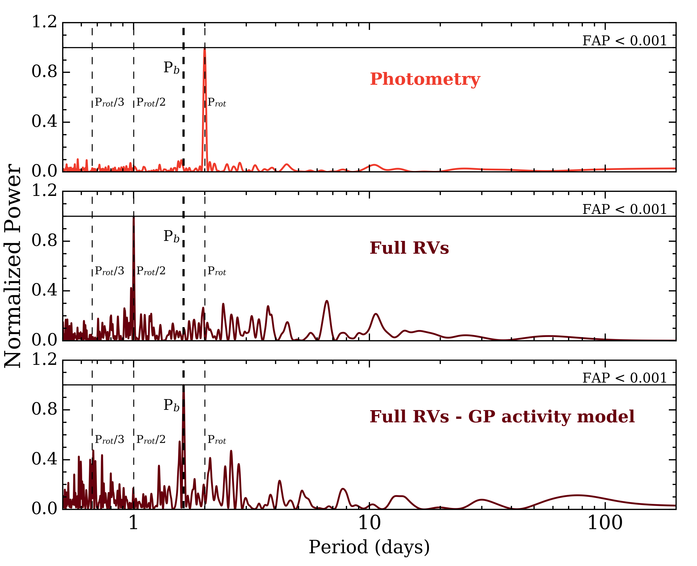
Figure 9.— Upper panel: Lomb-Scargle periodogram of the synthetic photometric light curve ($P_{\mathrm{rot}}=2$ days) Middle panel: Lomb-Scargle periodogram of the raw RV timeseries containing contributions from active regions and a planet with an orbital period distinct from $P_{\mathrm{rot}}$ ($P\sim 1.63$ days). Lower panel: the Lomb-Scargle periodogram of the RV residual timeseries after the subtraction of the mean Gaussian process activity model trained on the photometry. Upper limits on the false-alarm probability of significant peaks are highlighted by the horizontal solid lines. Vertical dashed lines highlight the injected planetary orbital period and the stellar rotation period plus its first and second harmonic periods.

Once we remove the GP jitter model from the observed RVs, the Lomb-Scargle periodogram exhibits a new distinct peak at $P_{b}\sim 1.63$ days (FAP $<0.1$%; lower panel Fig. 9). This is by far the strongest peak in the residual timeseries and leads to the detection of the periodic planetary signal with high significance. This test further demonstrates the effectiveness of using Gaussian processes to detect low-amplitude planetary signals around active stars in RV if additional, activity-sensitive timeseries are obtained either contemporaneously or in quick succession to RV observations in order to avoid any discrepancies that may arise from long-timescale activity cycles.

5.3. Improving the Mass Estimate of GJ 1132b with Large N_obs

A natural consequence of obtaining large values of N_obs to detect additional planets around GJ 1132 is that the semiamplitude $K_{b}$ can be better constrained in the process. For example, using just the 25 published RV measurements (B15), the semiamplitude and planet mass $m_{p,b}$ are detected at a level of $\sim 3.4\sigma$. Here we compute the planet mass detection significance of GJ 1132b for increased values of N_obs. To avoid spurious effects on the planet mass measurement brought on by specific window functions, we use multiple draws of orbital phase to create multiple timeseries. We then fit the dataset with a single keplarian model using MCMC with the orbital period and time of mid-transit constrained by narrow uniform priors based on the uncertainties listed in Table 1. The prior of $K_{b}$ is uniform on $[0,15]$ m s^-1. The $16^{\mathrm{th}}$ and $84^{\mathrm{th}}$ percentiles of the $K_{b}$ posterior distribution are used to compute its uncertainty which is then used along with the relevant values from Table 1 to compute the planet mass, its uncertainty, and hence its detection significance. The results are shown in Fig. 10.

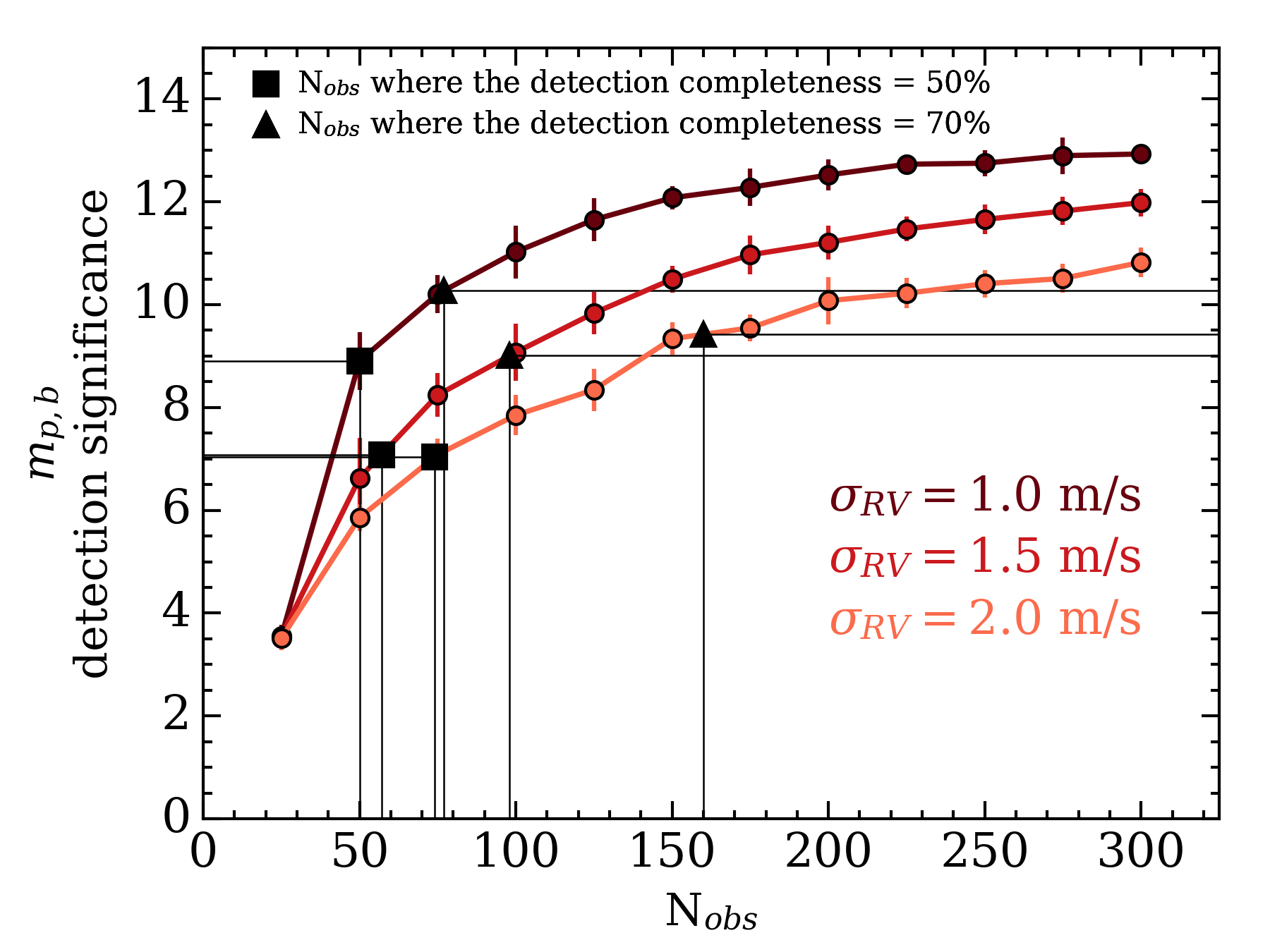
Figure 10.— The detection significance of the GJ 1132b planet mass of various RV measurement uncertainties. Errorbars result from the dispersion in values of $m_{p,b}$ when various window functions are used. The value of N_obs for which the detection completeness of all planets is 50% (squares) and 70% (triangles; see Fig. 4) is depicted with vertical lines for each value of $\sigma_{\mathrm{RV}}$.

For N_obs $=25$ the detection significance is independent of $\sigma_{\mathrm{RV}}$ because the dataset only includes the published radial velocities whose noise properties are fixed. When $\sigma_{\mathrm{RV}}=1$ m s^-1, a bona fide mass detection of 5$\sigma$ ($10\sigma$) is achieved for GJ 1132b with N_obs $\sim 32$ ($\sim 70$). When $\sigma_{\mathrm{RV}}$ is increased to 2 m s^-1, a $5\sigma$ ($10\sigma$) mass detection requires N_obs $\sim 40$ ($\sim 200$).

Fig. 10 also shows the mass detection significance obtained after a sufficient number of RV observations have been obtained in order to reach a 50% and 70% planet detection completeness. For instance, for $\sigma_{\mathrm{RV}}=1$ m s^-1, when we are 50% (70%) complete to additional planets in the system, the mass of GJ 1132b can be measured at the $\sim 9\sigma$ ($\sim 10\sigma$) level. Similarly for $\sigma_{\mathrm{RV}}=2$ m s^-1, when we are 50% (70%) complete to additional planets in the system, the mass of GJ 1132b can be measured at the $\sim 7\sigma$ ($\sim 9\sigma$). This assumes that the signal from additional planets have either a small RV signal or that they can be modelled with sufficient accuracy such that the residual rms is not large compared to the RV measurement uncertainty.

5.4. Effect of Varying the Mass-Radius Relationship

Throughout this work we have assumed a simplistic mass-radius relationship which assigns a bulk density equivalent to that of the Earth for small planets ($r_{p}\leq 1.6$ R_⊕) and the bulk density of Neptune for larger planets. This adopted relationship is not intended to be representative of the empirical distribution of planet masses and radii given that nature appears to present us with a range of planetary radii for given a mass (Seager et al., 2007; Zeng & Sasselov, 2013). Rather, we chose this relationship because of its simplicity and to remain agnostic regarding the exact form of the relationship between planetary mass and radius. Indeed many deterministic and probabilistic relations have been proposed.

However, it is worth noting how our detection completeness changes if a different mass-radius relation is adopted. We test this using the two-regime fit from Weiss & Marcy (2014) (hereafter WM14) which allows the bulk density of rocky planets to increase linearly with $r_{p}$ for $r_{p}<1.5$ R_⊕. The relation then switches to a $m_{p}\propto r_{p}^{0.93}$ powerlaw for larger planets up to 4 R_⊕. Each regime has an intrinsic scatter about the best-fit model which makes the relationship probabilistic. We use the model parameters reported in WM14 to convert our sample of planet radii to masses and re-compute the detection completeness using this new sample of planet masses.

The discrepancies that arise from adopting different mass-radius relationships are illustrated in Fig. 11. Firstly, taking a subset of 1000 planet radii from our MC sample, we compute the planet masses using each relationship and plot the resulting masses against each other in the top panel of Fig. 11. It is clear that the WM14 planet masses are frequently greater than the resulting mass when assuming a constant bulk density. For a given $r_{p}$, WM14 returns a larger $m_{p}$ than our adopted mass-radius relationship in $\sim 75$% of cases. This translates into a detection completeness which is greater than that which was previously obtained in our full MC simulation. The lower panel of Fig. 11 demonstrates that the detection completeness increases by $\sim 10-25$% if we adopt the WM14 mass-radius relation thus, on average obtaining larger $m_{p}$ from our sample of $r_{p}$. Therefore, the fiducial mass-radius relation used in our study represents a conservative case as adopting a different mass-radius relation based on the empirical distribution of planets will yield higher mass planets thus making them easier to detect in RV.

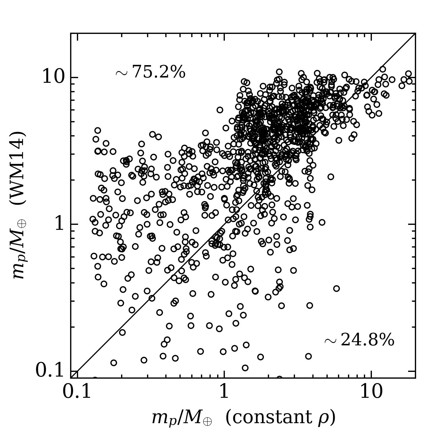
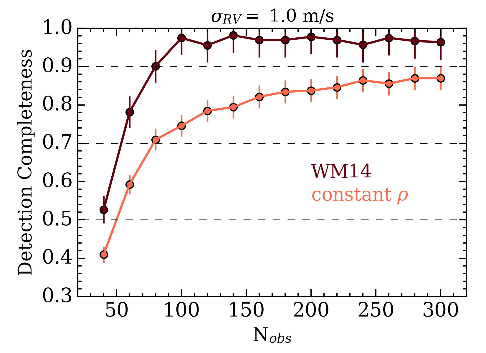
Figure 11.— Top panel: the masses predicted by two planetary mass-radius relations: i) constant bulk density equal to either Earth or Neptune depending on the planet size; the relation used for the majority of this work or ii) the two-regime fit to the empirical planet distribution from Weiss & Marcy (2014). Bottom panel: the detection of planets around GJ 1132 for the two planetary mass-radius relationships.

5.5. Detection Completeness for Planet Population Statistics

We noted in Sect. 5.1 that the planet detection completeness curves shown in Figs. 4, 5, and 6 will be applicable to a significant number ($\sim 280$) of TESS systems with planet candidates. In other words, the detection completeness of nearly edge-on, small planets around slowly rotating M-dwarfs has, to a good approximation, been computed using GJ 1132 as a test case. The detection completeness as a function of RV measurements is useful when attempting to infer global properties of a planet population. In particular, for the aforementioned TESS systems, our detection completeness, coupled with the results of RV follow-up observations contains information on the number of planets in a given system. This is true given that the known occurrence rates of planets around M-dwarfs was naturally folded into our MC simulations and therefore into our detection completeness curves.

6. Summary and Conclusions

This study aims at investigating the detection completeness of small planets around slowly rotating M-dwarfs when the planetary system is orientated nearly edge-on using precision radial velocity (RV) measurements. This will be the case for a large subset of TESS candidate systems which will contain at least one transiting planet requiring follow-up observations to characterize the planet’s mass and to search for additional planets in the system not seen to transit. In practise, we perform this calculation using GJ 1132 as a fiducial test case. Using existing photometric and RV data of this nearby M-dwarf and its short-period rocky companion GJ 1132b, we simulate the expected RV signal of the star at future epochs and compute the detection completeness of additional planetary companions in the system under realistic observing conditions. Our main results are as follows.

• Using a non-parametric Gaussian process to model the star’s photometric variability, we measure a stellar rotation period $P_{\mathrm{rot}}\sim 122$ days, consistent with previous estimates (Berta-Thompson et al., 2015), and predict that the associated level of RV jitter to be $\sim 8$ m s^-1. A Gaussian process model is used to model the jitter down to a residual rms value comparable to the RV stability limit of 1 m s^-1.

• We run a intensive suite of Monte-Carlo simulations which computes the expected RV signal from stellar jitter and small planets, sampled from their known occurrence rates, and quantifies the planet detection completeness as a function of the number of RV measurements.

• We find that the detection completeness of all additional planets (excluding the known transiting planet), is $\sim 80-85$% and is achieved with $\sim 200$ measurements for a nominal RV measurement uncertainty of $\sigma_{\mathrm{RV}}=1$ m s^-1. Increasing $\sigma_{\mathrm{RV}}$ by a factor of 2 only worsens the detection completeness by $\sim 10-15$%.

• For a given number of measurements and RV measurement uncertainty, the detection completeness of potentially habitable worlds is found to be consistent with the detection completeness to the full planet sample.

• Limits on the number of RV measurements required to recover 50% of i) all potential planets in the system and ii) all potentially habitable planets with state-of-the-art instrumentation is N_obs $\sim 50$.

• If contemporaneous ancillary timeseries, such as photometry, can be obtained, then the use of Gaussian processes are a powerful tool of modelling stellar jitter in active stars and detecting small amplitude planets.

Our detection completeness curves may also be applied to other slowly rotating M-dwarf systems containing at least one transiting planet such as those which will be found with TESS. Knowledge of planet detection completeness as a function of the number of RV observations is incredibly useful for optimizing observing strategies aimed at the efficient detection of large samples of exoplanets. For cases in which planetary systems exist around active (often rapidly rotating) M-dwarfs, we recommend the use of Gaussian processes to distinguish between jitter and dynamical signals if ancillary timeseries such as photometry, polarimetry, multi-wavelength RV measurements, and/or spectral activity indicators (e.g. $\log{R_{\mathrm{HK}}^{\prime}}$ or H$\alpha$) can also be obtained.

Appendix A Modelling the photometric variability of GJ 1132 with a Gaussian process

Gaussian process (GP) regression is an attractive method for modelling the complex stochastic processes contributing to stellar variability and naturally lends itself to the class of Bayesian inferential statistics. Thus it is extremely well-suited to the computation of model hyperparameter values and uncertainties and has recently been applied in the literature to the recovery of stellar rotation periods (e.g. Angus et al., 2015; Mancini et al., 2015; Vanderburg et al., 2015) and to the modelling of RV jitter from spectroscopic activity diagnostics (e.g. Rajpaul et al., 2015) or photometry of active stars (e.g. Haywood et al., 2014; Grunblatt et al., 2015).

Motivated by previous observational studies (e.g. Grunblatt et al., 2015; Mancini et al., 2015; Vanderburg et al., 2015) and the notion that photometric variations due to rotating active regions evolve in a quasi-periodic (QP) manner, we adopt a QP covariance function, or kernel, to describe the correlation between pairs of measurements. Explicitly, the time-correlation between data points is modelled as

$$k_{i,j}=a^{2}\exp{\left[-\frac{|x_{i}-x_{j}|^{2}}{2\lambda^{2}}-\Gamma^{2}\sin^{2}{\left(\frac{\pi|x_{i}-x_{j}|}{P_{\mathrm{rot}}}\right)}\right]},$$ (A1)

where $x_{i}$ is the independent measurement epoch of the $i^{\mathrm{th}}$ measurement where the indices $i,j=1,\dots,N$ and $N$ is the number of data points. This covariance function is parameterized by four GP hyperparameters: the amplitude of the correlations $a$, the exponential decay timescale $\lambda$, the coherence ‘scale’ of the correlations $\Gamma$, and the timescale of the periodic term $P_{\mathrm{rot}}$ which is representative of the stellar rotation period when using the QP GP regression model to model the star’s photometric variability. As mentioned, this kernel function is commonly used to model stellar light curves in a non-parametric way and returns the stellar rotation period, an important measurable property of the star, as a by-product of sampling the GP hyperparameters.

To sample the probability distribution functions of the GP hyperparameters we ran a Markov chain Monte-Carlo (MCMC) simulation using the MEarth photometric light curve (Fig. 1), re-sampled in 4 day bins to reduce the simulation’s computational expense ($\mathcal{O}(N^{3})$). The MCMC simulation was run using the affine-invariant MCMC ensemble sampler emcee (Foreman-Mackey et al., 2013) coupled with the fast GP package george (Ambikasaran et al., 2014; Foreman-Mackey, 2015) which is used to perform the necessary matrix inversions (see Eq. A2). Throughout the MCMC the acceptance fraction of the sampler is monitored and constrained to $\sim 25-50$%. Furthermore, we insist that the length of each Markov chain is at least a few ($\sim 10$) autocorrelation times such that we obtain multiple independent samples of each hyperparameter’s marginalized posterior probability distribution function.

The logarithmic likelihood function to be optimized by the MCMC is

$$\ln{\mathcal{L}}=-\frac{1}{2}\left(\mathbf{y}^{T}K^{-1}\mathbf{y}+\ln{\mathrm{det}K}+N\ln{2\pi}\right)$$ (A2)

where the $N\times N$ covariance matrix $K$ is

$$K_{i,j}=\sigma_{i}^{2}\delta_{i,j}+k_{i,j}.$$ (A3)

In our case the vector $\mathbf{y}$ contains the $N$ differential magnitude measurements with variance $\sigma^{2}_{i}$ for the $i^{\mathrm{th}}$ measurement which are assumed to be uncorrelated. The $\delta_{i,j}$ denotes the Kronecker delta.

The marginalized posterior probabilities for each hyperparameter are calculated up to a constant via the sum of Eq. A2 with a uniform logarithmic prior on each hyperparameter. All hyperparameters excluding $\lambda$ are effectively unconstrained by their broad uniform prior. From initial tests in which $\lambda$ is also left effectively unconstrained by a strict prior, a bi-modal $\lambda$ marginalized posterior distribution was observed which resulted in a corresponding value of $P_{\mathrm{rot}}$ not being well-defined. Each peak in the bi-modal $\lambda$ posterior was centered on a timescale greater than the expected stellar rotation period ($P_{\mathrm{rot}}\sim 125$ days; B15, ) implying a long exponential decay timescale overlaid with the rotationally induced periodicity. By constructing two separate (uniform) priors on $\lambda$ that each spanned the values of one of the aforementioned peaks, we found that focusing on the first bi-modal peak (i.e. the shorter timescale peak) prevented a well-defined solution for $P_{\mathrm{rot}}$ from being found. Consequently, we limit $\ln{\lambda}>8.5$ thus focusing on the second, longer timescale peak in the bi-modal distribution. The result is well-defined values for all hyperparameters. A similar effect was found in Rajpaul et al. (2015) wherein restriction of the timescale $\lambda$ to values greater than some threshold prevented the convergence of $P_{\mathrm{rot}}$ to unphysical, short timescale ‘contortions’. The resulting marginalized and joint hyperparameter posteriors are shown in Fig. 12.

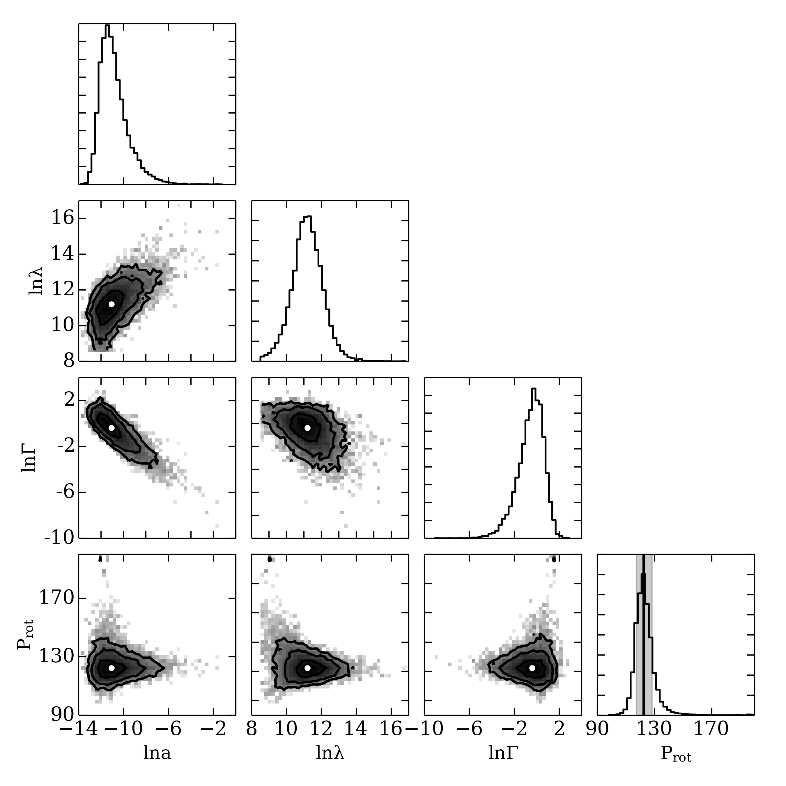
Figure 12.— Marginalized and joint posteriors for the quasi-periodic Gaussian process hyperparameters. Only $\lambda$ is constrained by a strict uniform prior of $\ln{\lambda}>8.5$. All hyperparameters are well-constrained by the MEarth photometry including a measured stellar rotation of $P_{\mathrm{rot}}=122.31^{+6.03}_{-5.04}$ days.

As an aside, we note that the MAP solution for $\lambda=7.26\times 10^{4}$ days is two orders of magnitude greater than the time baseline for the MEarth observations ($\sim 544$ days). Therefore, this timescale is not well-constrained by the data and additional photometry for the star is required to achieve a robust measurement of its value. Given the nature of the hyperparameter $\lambda$, the only remaining hyperparameter with a physical interpretation is $P_{\mathrm{rot}}$ whose marginalized posterior probability is shown in the bottom right panel of Fig. 12. From its posterior we measure the MAP value of the stellar rotation period to be $P_{\mathrm{rot}}=122.31^{+6.03}_{-5.04}$ days where the quoted uncertainties are based on the $16^{\mathrm{th}}$ and $84^{\mathrm{th}}$ percentiles. This result from the GP regression analysis is consistent with the measured rotation of $\sim 125$ days from B15 determined using the sine-wave fitting methodology of Irwin et al. (2011) and Newton et al. (2016b).

Appendix B Planet detection via Bayesian model selection

Here we discuss the Bayesian model selection framework and its application to detecting planets in our Monte-Carlo (MC) simulations.

Firstly, we denote a complete dataset by the vector $\mathbf{D}$ containing $N_{\mathrm{obs}}$ RV measurements each with an associated error and taken at a unique BJD. These data are assumed to be derived from one of three proposed models (or hypotheses) denoted $M_{k}$ where $k=0,1,2$ denotes the number of planets in the model. The model $M_{0}$ is referred to as the null hypothesis to which we can compare other models of increasing complexity, to test their validity. Each model has a corresponding set of unique model parameters $\mathbf{\Theta}_{k}$ with dimensionality $D$. For models with $k>0$, the set of model parameters $\mathbf{\Theta}_{k}$ includes each planets’ orbital period, time of mid-transit, and semiamplitude. All orbits are assumed to be circular to simplify the modelling process.

Bayes theorem tells us that

$$\mathrm{P}(\mathbf{\Theta}_{k}|\mathbf{D},M_{k})=\frac{\mathrm{P}(\mathbf{D}|\mathbf{\Theta}_{k},M_{k})\cdot\mathrm{P}(\mathbf{\Theta}_{k}|M_{k})}{\mathrm{P}(\mathbf{D}|M_{k})},$$ (B1)

where $\mathrm{P}(\mathbf{\Theta}_{k}|\mathbf{D},M_{k})$ is the posterior probability of the $M_{k}$ model parameters, $\mathrm{P}(\mathbf{D}|\mathbf{\Theta}_{k},M_{k})\equiv\mathcal{L}$ is the likelihood of obtaining the observed data given a set of model parameters, $\mathrm{P}(\mathbf{\Theta}_{k}|M_{k})$ is the prior on the model parameters, and $\mathrm{P}(\mathbf{D}|M_{k})\equiv Z$ is a normalization factor equal to the evidence for the model $M_{k}$. In general, computation of model evidences is not required for parameter estimation only but is necessary for model comparison and selection in our MC simulations.

To determine which model best describes a dataset one must calculate the marginal model posterior probabilities $\mathrm{P}(M_{k}|\mathbf{D})$ for each model $M_{k}$. The ratio of these values for two competing models in known as the Bayes factor and is commonly used to infer which model is most favorable for describing a dataset. Therefore, for arbitrary models designated $M_{m}$ and $M_{n}$, the Bayes factor is

$$R_{mn}\equiv\frac{\mathrm{P}(M_{m}|\mathbf{D})}{\mathrm{P}(M_{n}|\mathbf{D})}$$ (B2)

where,

$$\mathrm{P}(M_{k}|\mathbf{D})=\frac{\mathrm{P}(\mathbf{D}|M_{k})\cdot\mathrm{P}(M_{k})}{\sum_{k}\mathrm{P}(\mathbf{D}|M_{k})\cdot\mathrm{P}(M_{k})}$$ (B3)

is the probability that the model $M_{k}$ describes the data. The factor in the denominator of Eq. B3 contains a summation over all model evidences considered and therefore cancels when computing Bayes factors using Eq. B2. This cancellation allows us to write the Bayes factor describing the evidence for a model $M_{m}$ compared to $M_{n}$ as

$$R_{mn}=\frac{\mathrm{P}(\mathbf{D}|M_{m})}{\mathrm{P}(\mathbf{D}|M_{n})}\frac{\mathrm{P}(M_{m})}{\mathrm{P}(M_{n})}.$$ (B4)

Throughout this study we fix the ratio $\mathrm{P}(M_{m})/\mathrm{P}(M_{n})$ to unity for all $m,n$ to ensure that we are not biased towards any particular number of keplarians. This is intended to representative of the GJ 1132 case wherein although we expect there to be additional planets in the system based on the high frequency of small planets around M-dwarfs (Dressing & Charbonneau, 2013, 2015), increasing this ratio to $\mathrm{P}(M_{k>1})/\mathrm{P}(M_{k=1})>1$ would favor additional planets which may or may not actually be present. The model evidences are then obtained by integrating over the model’s full parameter space:

$$Z_{k}\equiv\mathrm{P}(\mathbf{D}|M_{k})=\int\mathcal{L}\cdot\mathrm{P}(\mathbf{\Theta}_{k}|M_{k})\cdot\mathrm{d}^{D}\mathbf{\Theta}_{k}.$$ (B5)

Evaluation of the multi-dimensional integral in Eq. B5 is an intensive computational task. To evaluate this integral for each model $M_{k}$ with $k=0,1,2$, we use the Multinest (Feroz & Hobson, 2008; Feroz et al., 2009; Feroz & Hobson, 2014) nested sampling algorithm given the logarithmic likelihood function

$$\log{}\mathcal{L}=-\frac{1}{2}\sum_{i=1}^{N_{\mathrm{obs}}}\left(\frac{(y_{i}-\mathrm{model}_{i})}{\sigma_{i}}\right)^{2}-\log{\left(\frac{1}{\sigma_{i}^{2}}\right)}$$ (B6)

and appropriately chosen model parameter priors. The values $y_{i}$ and $\sigma_{i}$ denote the observed RV and its uncertainty respectively while model_i is the value of the model $M_{k}$ for the measurement $i$ determined by the parameters $\mathbf{\Theta}_{k}$.

As discussed in Sect. 3.4, the $M_{1}$ model parameter priors are based on the measured values for GJ 1132b in Table 1 whilst the prior on the orbital period for any additional planet is based on any low false-alarm probability peak in a Lomb-Scargle periodogram $P_{\mathrm{peak}}$ of the RV residuals (GJ 1132 b keplarian removed). Priors on $T0_{c}$ and $K_{c}$ are left broad and uniform; $T0_{c}\in[T0_{b}-P_{\mathrm{peak}}/2,T0_{b}+P_{\mathrm{peak}}/2]$ BJD and $K_{c}\in(0,15]$ m s^-1. Detection of a second planet therefore requires a periodogram periodicity detection coupled with a favorable Bayes factor of the two planet model compared to the single planet model; $R_{21}>20$ (Kass & Raftery, 1995).

References

- Agol et al. (2005) Agol, E., Steffen, J., Sari, R., & Clarkson, W. 2005, MNRAS, 359, 567
- Aigrain et al. (2012) Aigrain, S., Pont, F., & Zucker, S. 2012, MNRAS, 419, 3147
- Ambikasaran et al. (2014) Ambikasaran, S., Foreman-Mackey, D., Greengard, L., Hogg, D. W., & O’Neil, M. 2014, ArXiv e-prints, arXiv:1403.6015
- Angus et al. (2015) Angus, R., Aigrain, S., & Foreman-Mackey, D. 2015, IAU General Assembly, 22, 2258396
- Artigau et al. (2014) Artigau, É., Kouach, D., Donati, J.-F., et al. 2014, in Society of Photo-Optical Instrumentation Engineers (SPIE) Conference Series, Vol. 9147, Society of Photo-Optical Instrumentation Engineers (SPIE) Conference Series, 15
- Baluev (2008) Baluev, R. V. 2008, MNRAS, 385, 1279
- Baluev (2013) —. 2013, MNRAS, 429, 2052
- Barnes et al. (2005) Barnes, J. R., Collier Cameron, A., Donati, J.-F., et al. 2005, MNRAS, 357, L1
- Barnes & Greenberg (2006) Barnes, R., & Greenberg, R. 2006, ApJ, 647, L163
- Barnes (2003) Barnes, S. A. 2003, ApJ, 586, 464
- Barnes (2007) —. 2007, ApJ, 669, 1167
- Bean et al. (2013) Bean, J. L., Désert, J.-M., Seifahrt, A., et al. 2013, ApJ, 771, 108
- Beichman et al. (2014) Beichman, C., Benneke, B., Knutson, H., et al. 2014, PASP, 126, 1134
- Berta-Thompson et al. (2015) Berta-Thompson, Z. K., Irwin, J., Charbonneau, D., et al. 2015, Nature, 527, 204
- Bonfils et al. (2007) Bonfils, X., Mayor, M., Delfosse, X., et al. 2007, A&A, 474, 293
- Bonfils et al. (2013) Bonfils, X., Delfosse, X., Udry, S., et al. 2013, A&A, 549, A109
- Bouchy et al. (2001) Bouchy, F., Pepe, F., & Queloz, D. 2001, A&A, 374, 733
- Brown (2001) Brown, T. M. 2001, ApJ, 553, 1006
- Browning et al. (2010) Browning, M. K., Basri, G., Marcy, G. W., West, A. A., & Zhang, J. 2010, AJ, 139, 504
- Charbonneau (2015) Charbonneau, D. 2015, in AAS/Division for Extreme Solar Systems Abstracts, Vol. 3, AAS/Division for Extreme Solar Systems Abstracts, 101.01
- Christensen-Dalsgaard (2004) Christensen-Dalsgaard, J. 2004, Sol. Phys., 220, 137
- Cloutier et al. (2015) Cloutier, R., Tamayo, D., & Valencia, D. 2015, ApJ, 813, 8
- Cloutier & Triaud (2016) Cloutier, R., & Triaud, A. H. M. J. 2016, MNRAS, 462, 4018
- Cowan et al. (2012) Cowan, N. B., Voigt, A., & Abbot, D. S. 2012, ApJ, 757, 80
- Crouzet et al. (2014) Crouzet, N., McCullough, P. R., Deming, D., & Madhusudhan, N. 2014, ApJ, 795, 166
- Cumming (2004) Cumming, A. 2004, MNRAS, 354, 1165
- Delfosse et al. (2013) Delfosse, X., Donati, J.-F., Kouach, D., et al. 2013, in SF2A-2013: Proceedings of the Annual meeting of the French Society of Astronomy and Astrophysics, ed. L. Cambresy, F. Martins, E. Nuss, & A. Palacios, 497–508
- Dole (1964) Dole, S. H. 1964, Habitable planets for man
- Dressing & Charbonneau (2013) Dressing, C. D., & Charbonneau, D. 2013, ApJ, 767, 95
- Dressing & Charbonneau (2015) —. 2015, ApJ, 807, 45
- Dressing et al. (2010) Dressing, C. D., Spiegel, D. S., Scharf, C. A., Menou, K., & Raymond, S. N. 2010, ApJ, 721, 1295
- Dressing et al. (2015) Dressing, C. D., Charbonneau, D., Dumusque, X., et al. 2015, ApJ, 800, 135
- Dumusque et al. (2011) Dumusque, X., Udry, S., Lovis, C., Santos, N. C., & Monteiro, M. J. P. F. G. 2011, A&A, 525, A140
- Duncan et al. (1989) Duncan, M., Quinn, T., & Tremaine, S. 1989, Icarus, 82, 402
- Fabrycky et al. (2012) Fabrycky, D. C., Ford, E. B., Steffen, J. H., et al. 2012, ApJ, 750, 114
- Fabrycky et al. (2014) Fabrycky, D. C., Lissauer, J. J., Ragozzine, D., et al. 2014, ApJ, 790, 146
- Feroz & Hobson (2008) Feroz, F., & Hobson, M. P. 2008, MNRAS, 384, 449
- Feroz & Hobson (2014) —. 2014, MNRAS, 437, 3540
- Feroz et al. (2009) Feroz, F., Hobson, M. P., & Bridges, M. 2009, MNRAS, 398, 1601
- Figueira et al. (2012) Figueira, P., Marmier, M., Boué, G., et al. 2012, A&A, 541, A139
- Figueira et al. (2016) Figueira, P., Adibekyan, V. Z., Oshagh, M., et al. 2016, A&A, 586, A101
- Ford & Gregory (2007) Ford, E. B., & Gregory, P. C. 2007, in Astronomical Society of the Pacific Conference Series, Vol. 371, Statistical Challenges in Modern Astronomy IV, ed. G. J. Babu & E. D. Feigelson, 189
- Foreman-Mackey (2015) Foreman-Mackey, D. 2015, George: Gaussian Process regression, Astrophysics Source Code Library, ascl:1511.015
- Foreman-Mackey et al. (2013) Foreman-Mackey, D., Hogg, D. W., Lang, D., & Goodman, J. 2013, PASP, 125, 306
- Forveille et al. (2009) Forveille, T., Bonfils, X., Delfosse, X., et al. 2009, A&A, 493, 645
- Gaidos et al. (2016) Gaidos, E., Mann, A. W., Kraus, A. L., & Ireland, M. 2016, MNRAS, 457, 2877
- Gilliland & Baliunas (1987) Gilliland, R. L., & Baliunas, S. L. 1987, ApJ, 314, 766
- Gladman (1993) Gladman, B. 1993, Icarus, 106, 247
- Gray (2009) Gray, D. F. 2009, ApJ, 697, 1032
- Grunblatt et al. (2015) Grunblatt, S. K., Howard, A. W., & Haywood, R. D. 2015, ApJ, 808, 127
- Hart (1979) Hart, M. H. 1979, Icarus, 37, 351
- Haywood et al. (2014) Haywood, R. D., Collier Cameron, A., Queloz, D., et al. 2014, MNRAS, 443, 2517
- Haywood et al. (2016) Haywood, R. D., Collier Cameron, A., Unruh, Y. C., et al. 2016, MNRAS, 457, 3637
- Huélamo et al. (2008) Huélamo, N., Figueira, P., Bonfils, X., et al. 2008, A&A, 489, L9
- Irwin et al. (2011) Irwin, J., Berta, Z. K., Burke, C. J., et al. 2011, ApJ, 727, 56
- Irwin et al. (2015) Irwin, J. M., Berta-Thompson, Z. K., Charbonneau, D., et al. 2015, in Cambridge Workshop on Cool Stars, Stellar Systems, and the Sun, Vol. 18, 18th Cambridge Workshop on Cool Stars, Stellar Systems, and the Sun, ed. G. T. van Belle & H. C. Harris, 767–772
- Kane et al. (2012) Kane, S. R., Ciardi, D. R., Gelino, D. M., & von Braun, K. 2012, MNRAS, 425, 757
- Kass & Raftery (1995) Kass, R. E., & Raftery, A. E. 1995, Journal of the American Statistical Association, 90, 773
- Kasting et al. (1993) Kasting, J. F., Whitmire, D. P., & Reynolds, R. T. 1993, Icarus, 101, 108
- Kipping (2013) Kipping, D. M. 2013, MNRAS, 434, L51
- Kokubo et al. (2006) Kokubo, E., Kominami, J., & Ida, S. 2006, ApJ, 642, 1131
- Kopparapu et al. (2013) Kopparapu, R. K., Ramirez, R., Kasting, J. F., et al. 2013, ApJ, 765, 131
- Kotani et al. (2014) Kotani, T., Tamura, M., Suto, H., et al. 2014, in Proc. SPIE, Vol. 9147, Ground-based and Airborne Instrumentation for Astronomy V, 914714
- Kreidberg et al. (2014) Kreidberg, L., Bean, J. L., Désert, J.-M., et al. 2014, Nature, 505, 69
- Lopez & Fortney (2014) Lopez, E. D., & Fortney, J. J. 2014, ApJ, 792, 1
- Lovis et al. (2005) Lovis, C., Mayor, M., Bouchy, F., et al. 2005, A&A, 437, 1121
- Mahadevan et al. (2012) Mahadevan, S., Ramsey, L., Bender, C., et al. 2012, in Proc. SPIE, Vol. 8446, Ground-based and Airborne Instrumentation for Astronomy IV, 84461S
- Mahmud et al. (2011) Mahmud, N. I., Crockett, C. J., Johns-Krull, C. M., et al. 2011, ApJ, 736, 123
- Mancini et al. (2015) Mancini, L., Giacobbe, P., Littlefair, S. P., et al. 2015, A&A, 584, A104
- Marchal & Bozis (1982) Marchal, C., & Bozis, G. 1982, Celestial Mechanics, 26, 311
- Martín et al. (2006) Martín, E. L., Guenther, E., Zapatero Osorio, M. R., Bouy, H., & Wainscoat, R. 2006, ApJ, 644, L75
- Mayor et al. (2003) Mayor, M., Pepe, F., Queloz, D., et al. 2003, The Messenger, 114, 20
- McCullough et al. (2014) McCullough, P. R., Crouzet, N., Deming, D., & Madhusudhan, N. 2014, ApJ, 791, 55
- McQuillan et al. (2013a) McQuillan, A., Aigrain, S., & Mazeh, T. 2013a, MNRAS, 432, 1203
- McQuillan et al. (2013b) McQuillan, A., Mazeh, T., & Aigrain, S. 2013b, ApJ, 775, L11
- McQuillan et al. (2014) —. 2014, ApJS, 211, 24
- Meschiari et al. (2009) Meschiari, S., Wolf, A. S., Rivera, E., et al. 2009, PASP, 121, 1016
- Mohanty & Basri (2003) Mohanty, S., & Basri, G. 2003, ApJ, 583, 451
- Newton et al. (2016a) Newton, E. R., Irwin, J., Charbonneau, D., Berta-Thompson, Z. K., & Dittmann, J. A. 2016a, ApJ, 821, L19
- Newton et al. (2016b) Newton, E. R., Irwin, J., Charbonneau, D., et al. 2016b, ApJ, 821, 93
- Noyes et al. (1984) Noyes, R. W., Hartmann, L. W., Baliunas, S. L., Duncan, D. K., & Vaughan, A. H. 1984, ApJ, 279, 763
- O’Neal et al. (2005) O’Neal, D., Saar, S. H., Neff, J. E., & Cuntz, M. 2005, in ESA Special Publication, Vol. 560, 13th Cambridge Workshop on Cool Stars, Stellar Systems and the Sun, ed. F. Favata, G. A. J. Hussain, & B. Battrick, 853
- Payne et al. (2010) Payne, M. J., Ford, E. B., & Veras, D. 2010, ApJ, 712, L86
- Prato et al. (2008) Prato, L., Huerta, M., Johns-Krull, C. M., et al. 2008, ApJ, 687, L103
- Quillen et al. (2007) Quillen, A. C., Morbidelli, A., & Moore, A. 2007, MNRAS, 380, 1642
- Quirrenbach et al. (2014) Quirrenbach, A., Amado, P. J., Caballero, J. A., et al. 2014, in Proc. SPIE, Vol. 9147, Ground-based and Airborne Instrumentation for Astronomy V, 91471F
- Rajpaul et al. (2015) Rajpaul, V., Aigrain, S., Osborne, M. A., Reece, S., & Roberts, S. 2015, MNRAS, 452, 2269
- Raymond et al. (2005) Raymond, S. N., Quinn, T., & Lunine, J. I. 2005, ApJ, 632, 670
- Reiners & Basri (2007) Reiners, A., & Basri, G. 2007, ApJ, 656, 1121
- Reiners et al. (2010) Reiners, A., Bean, J. L., Huber, K. F., et al. 2010, ApJ, 710, 432
- Reiners et al. (2012) Reiners, A., Joshi, N., & Goldman, B. 2012, AJ, 143, 93
- Reiners & Mohanty (2012) Reiners, A., & Mohanty, S. 2012, ApJ, 746, 43
- Reiners et al. (2013) Reiners, A., Shulyak, D., Anglada-Escudé, G., et al. 2013, A&A, 552, A103
- Ricker et al. (2014) Ricker, G. R., Winn, J. N., Vanderspek, R., et al. 2014, in Proc. SPIE, Vol. 9143, Space Telescopes and Instrumentation 2014: Optical, Infrared, and Millimeter Wave, 914320
- Scargle (1982) Scargle, J. D. 1982, ApJ, 263, 835
- Schmidt et al. (2012) Schmidt, S. J., Kowalski, A. F., Hawley, S. L., et al. 2012, ApJ, 745, 14
- Seager et al. (2007) Seager, S., Kuchner, M., Hier-Majumder, C. A., & Militzer, B. 2007, ApJ, 669, 1279
- Selsis et al. (2007) Selsis, F., Kasting, J. F., Levrard, B., et al. 2007, A&A, 476, 1373
- Smith & Lissauer (2009) Smith, A. W., & Lissauer, J. J. 2009, Icarus, 201, 381
- Snellen (2013) Snellen, I. 2013, in European Physical Journal Web of Conferences, Vol. 47, European Physical Journal Web of Conferences, 11001
- Spiegel et al. (2008) Spiegel, D. S., Menou, K., & Scharf, C. A. 2008, ApJ, 681, 1609
- Spiegel et al. (2009) —. 2009, ApJ, 691, 596
- Stewart & Ida (2000) Stewart, G. R., & Ida, S. 2000, Icarus, 143, 28
- Sullivan et al. (2015) Sullivan, P. W., Winn, J. N., Berta-Thompson, Z. K., et al. 2015, ApJ, 809, 77
- Van Eylen & Albrecht (2015) Van Eylen, V., & Albrecht, S. 2015, ApJ, 808, 126
- Vanderburg et al. (2016) Vanderburg, A., Plavchan, P., Johnson, J. A., et al. 2016, MNRAS, 459, 3565
- Vanderburg et al. (2015) Vanderburg, A., Montet, B. T., Johnson, J. A., et al. 2015, ApJ, 800, 59
- Vladilo et al. (2013) Vladilo, G., Murante, G., Silva, L., et al. 2013, ApJ, 767, 65
- Weiss & Marcy (2014) Weiss, L. M., & Marcy, G. W. 2014, ApJ, 783, L6
- West et al. (2015) West, A. A., Weisenburger, K. L., Irwin, J., et al. 2015, ApJ, 812, 3
- Williams & Kasting (1997) Williams, D. M., & Kasting, J. F. 1997, Icarus, 129, 254
- Wright (2005) Wright, J. T. 2005, PASP, 117, 657
- Yang et al. (2014) Yang, J., Boué, G., Fabrycky, D. C., & Abbot, D. S. 2014, ApJ, 787, L2
- Yang et al. (2013) Yang, J., Cowan, N. B., & Abbot, D. S. 2013, ApJ, 771, L45
- Zeng & Sasselov (2013) Zeng, L., & Sasselov, D. 2013, PASP, 125, 227