Hot DA white dwarf model atmosphere calculations: Including improved Ni PI cross sections

Abstract

To calculate realistic models of objects with Ni in their atmospheres, accurate atomic data for the relevant ionization stages needs to be included in model atmosphere calculations. In the context of white dwarf stars, we investigate the effect of changing the Ni iv-vi bound-bound and bound-free atomic data has on model atmosphere calculations. Models including PICS calculated with autostructure show significant flux attenuation of up to $\sim 80$% shortward of 180Å  in the EUV region compared to a model using hydrogenic PICS. Comparatively, models including a larger set of Ni transitions left the EUV, UV, and optical continua unaffected. We use models calculated with permutations of this atomic data to test for potential changes to measured metal abundances of the hot DA white dwarf G191-B2B. Models including autostructure PICS were found to change the abundances of N and O by as much as $\sim 22$% compared to models using hydrogenic PICS, but heavier species were relatively unaffected. Models including autostructure PICS caused the abundances of N/O iv and v to diverge. This is because the increased opacity in the autostructure PICS model causes these charge states to form higher in the atmosphere, moreso for N/O v. Models using an extended line list caused significant changes to the Ni iv-v abundances. While both PICS and an extended line list cause changes in both synthetic spectra and measured abundances, the biggest changes are caused by using autostructure PICS for Ni.

1 Introduction

The presence of metals in white dwarf (WD) atmospheres can have dramatic effects on both the structure of the atmosphere, and the observed effective temperature ($T_{\mathrm{eff}}$). For example, these effects have been demonstrated convincingly by Barstow et al. (1998). The authors determined the $T_{\mathrm{eff}}$ and surface gravity (log $g$) of several hot DA white dwarfs using a set of model atmosphere grids, which were either pure H & He, or heavy metal-polluted. It was found that the $T_{\mathrm{eff}}$ determined using the pure H model grid was $\approx{4000-7000}$K higher than if a heavy metal-polluted model grid were used. Conversely, there was little to no difference in the measured log $g$ when using either model grid.

It can be inferred that the completeness of the atomic data supplied in model calculations might have a significant effect on the measured $T_{\mathrm{eff}}$. A study by Chayer et al. (1995) considered the effects of radiative levitation on the observed atmospheric metal abundances at different $T_{\mathrm{eff}}$ and log $g$. In addition, these calculations were done using Fe data sets of varying line content. It was found that the number of transitions included in the calculation greatly affected the expected Fe abundance in the atmosphere (cf. Chayer et al. 1995, Figure 11). This result implies that the macroscopic quantities determined in a white dwarf, such as metal abundance, are extremely sensitive to the input physics used to calculate the model grids. Therefore, this means that any atomic data that is supplied to the calculation must be as complete and accurate as possible in order to calculate the most representative model. While the Chayer et al. (1995) study considered only the variations in observed Fe abundance, it is reasonable to assume that the set of atomic data supplied may also have an impact on the $T_{\mathrm{eff}}$ and log $g$ measured.

Studies of white dwarf metal abundances, such as those of Barstow et al. (1998); Vennes & Lanz (2001); Preval et al. (2013), used model atmospheres incorporating the atomic data of Kurucz (1992) (Ku92 hereafter) in conjunction with photoionization cross-section (PICS) data from the Opacity Project (OP) for Fe, and approximate hydrogenic PICS for Ni. A more comprehensive dataset has since been calculated by Kurucz (2011) (Ku11 hereafter), containing a factor $\sim{10}$ more transitions and energy levels for Fe and Ni iv-vi than its predecessor. In Table 1 we give a comparison of the number of Fe and Ni iv-vii transitions available between Ku92 and Ku11. In both the Ku92 and Ku11 datasets, the energy levels etc were calculated using the Cowan Code (Cowan, 1981). Based on the work discussed above, it is prudent to explore the differences between model atmospheres calculated using the Ku92 and Ku11 transition data, and the effect this has on measurements made using such models.

Table 1: The number of lines present in the Ku92 and Ku11 atomic databases for Fe and Ni iv-vii.

Ion	No of lines 1992	No of lines 2011
Fe iv	1,776,984	14,617,228
Fe v	1,008,385	7,785,320
Fe vi	475,750	9,072,714
Fe vii	90,250	2,916,992
Ni iv	1,918,070	15,152,636
Ni v	1,971,819	15,622,452
Ni vi	2,211,919	17,971,672
Ni vii	967,466	28,328,012
Total	10,420,643	111,467,026

Ni v absorption features were first discovered in the hot DA white dwarfs G191-B2B and REJ2214-492 by Holberg et al. (1994) using high dispersion UV spectra from the International Ultraviolet Explorer (IUE). The authors derived Ni abundances of $\sim 1\times{10}^{-6}$ and $\sim 3\times{10}^{-6}$ as a fraction of H for G191-B2B and REJ2214-492 respectively. Compared to their measurements for Fe of $\sim 3\times{10}^{-5}$ and $\sim 1\times{10}^{-4}$ for G191-B2B and REJ2214-492 respectively, Ni is $\sim 3$% of the Fe abundance for these stars. Werner & Dreizler (1994) also found Ni in two other hot DA white dwarfs, namely Feige 24, and RE0623-377, measuring Ni abundances of $1-5\times{10}^{-6}$ and $1-5\times{10}^{-5}$, respectively. More recently, Preval et al. (2013) and Rauch et al. (2013) have measured Ni abundances for G191-B2B. Using Ni iv and v, Preval et al. (2013) found abundances of $3.24\times{10}^{-7}$ and $1.01\times{10}^{-6}$ respectively, while Rauch et al. (2013) measured a single Ni abundance of $6\times{10}^{-7}$.

To date, there has been no attempt to include representative PICS for Ni in white dwarf model atmosphere calculations. It is for this reason that we choose to focus on Ni, and examine the effects of both including new PI cross sections, and transition data. We structure our paper as follows; We first describe the atomic data calculations required to generate PICS for Ni iv-vi. Next, we describe the model atmosphere calculations performed, and the tests we conducted. We then discuss the results. Finally, we state our conclusions.

2 Atomic data calculations

The PICS data presented in this paper were calculated using the distorted wave atomic collision package autostructure (Badnell, 1986, 1997, 2011). autostructure is an atomic structure package that can model several aspects of an arbitrary atom/ion a priori, including energy levels, transition oscillator strengths, electron-impact excitation cross sections, PICS, and many others. autostructure is supplied with a set of configurations describing the number of electrons and the quantum numbers occupied for a given atom or ion. The wavefunction $P_{nl}$ for a particular configuration is obtained by solving the one particle Schrodinger equation

$$\left[\frac{d^{2}}{dr^{2}}-\frac{l(l+1)}{r^{2}}+2V_{\mathrm{Eff}}(r)+E_{nl}\right]P_{nl}=0,$$ (1)

where $n$ and $l$ are the principle and orbital angular momentum quantum numbers respectively, and $V_{\mathrm{Eff}}$ is an effective potential as described by Eissner & Nussbaumer (1969), which accounts for the presence of other electrons. Scaling parameters $\lambda_{nl}$ can be included to scale the radial coordinate, which are related to the effective charge ‘seen’ by a particular valence electron, and typically has a value close to unity. The $\lambda_{nl}$ can be varied according to the task. For an example, the parameters may be varied to minimise an energy functional, or they may be varied such that the difference between the calculated energy levels and a set of observed energy levels is minimised. Three coupling schemes are available in calculating the wavefunctions, dependent upon the resolution required, and the type of problem being considered. These are LS coupling (term resolved), intermediate coupling (IC, level resolved), or configuration average (CA, configuration resolved).

We use IC with the aim of reproducing the energy levels from Ku11 as closely as possible. The energy level structure is first determined by running autostructure with the configurations used by Ku11, listed in Table 2. With this information, 17 $\lambda_{nl}$ are then specified for orbitals 1s to 6s set initially to unity. The 1s parameter is fixed as it does not converge in the presence of relativistic corrections. The parameters were then varied to give as close agreement to the Ku11 data as possible. The result of parameter variation is given in Table 3.

Table 2: Configurations prior to photoionization used in the autostructure calculations. Configurations in bold typeset represent the ground state configuration. The columns $N_{\mathrm{config}}$, Levels, and Lines give the number of configurations used, and the number of energy levels and transitions generated respectively.

Ion	Configurations	$N_{\mathrm{config}}$	Levels	Lines
Ni iv	$\mathbf{3d^{7}}$, $3d^{6}4s$, $3d^{6}5s$,$3d^{6}6s$, $3d^{6}7s$, $3d^{6}8s$	85	37,860	32,416,571
	$3d^{6}9s$, $3d^{5}4s^{2}$, $3d^{5}4s5s$, $3d^{5}4s6s$, $3d^{5}4s7s$, $3d^{5}4s8s$
	$3d^{5}4s9s$, $3d^{4}4s^{2}5s$, $3d^{6}4d$, $3d^{6}5d$, $3d^{6}6d$, $3d^{6}7d$
	$3d^{6}8d$, $3d^{6}9d$, $3d^{5}4s4d$, $3d^{5}4s5d$, $3d^{5}4s6d$, $3d^{5}4s7d$
	$3d^{5}4s8d$, $3d^{5}4s9d$, $3d^{4}4s^{2}4d$, $3d^{5}4p^{2}$, $3d^{6}5g$, $3d^{6}6g$
	$3d^{6}7g$, $3d^{6}8g$, $3d^{6}9g$, $3d^{5}4s5g$, $3d^{5}4s6g$, $3d^{5}4s7g$
	$3d^{5}4s8g$, $3d^{5}4s9g$, $3d^{6}7i$, $3d^{6}8i$, $3d^{6}9i$, $3d^{5}4s7i$
	$3d^{5}4s8i$, $3d^{5}4s9i$
	$3d^{6}4p$, $3d^{6}5p$, $3d^{6}6p$, $3d^{6}7p$, $3d^{6}8p$, $3d^{6}9p$
	$3d^{5}4s4p$, $3d^{5}4s5p$, $3d^{5}4s6p$, $3d^{5}4s7p$, $3d^{5}4s8p$, $3d^{5}4s9p$
	$3d^{4}4s^{2}4p$, $3d^{6}4f$, $3d^{6}5f$, $3d^{6}6f$, $3d^{6}7f$, $3d^{6}8f$
	$3d^{6}9f$, $3d^{5}4s4f$, $3d^{5}4s5f$, $3d^{5}4s6f$, $3d^{5}4s7f$, $3d^{5}4s8f$
	$3d^{5}4s9f$, $3d^{4}4s^{2}4f$, $3d^{6}6h$, $3d^{6}7h$, $3d^{6}8h$, $3d^{6}9h$
	$3d^{5}4s6h$, $3d^{5}4s7h$, $3d^{5}4s8h$, $3d^{5}4s9h$, $3d^{6}8k$, $3d^{6}9k$
	$3d^{5}4s8k$, $3d^{5}4s9k$, $3p^{5}3d^{8}$
Ni v	$\mathbf{3d^{6}}$, $3d^{5}4d$, $3d^{5}5d$, $3d^{5}6d$, $3d^{5}7d$, $3d^{5}8d$	87	37,446	34,066,259
	$3d^{5}9d$, $3d^{5}10d$, $3d^{4}4s4d$, $3d^{4}4s5d$, $3d^{4}4s6d$, $3d^{4}4s7d$
	$3d^{4}4s8d$, $3d^{4}4s9d$, $3d^{4}4s10d$, $3d^{5}4s$, $3d^{5}5s$, $3d^{5}6s$
	$3d^{5}7s$, $3d^{5}8s$, $3d^{5}9s$, $3d^{5}10s$, $3d^{4}4s^{2}$, $3d^{4}4s5s$
	$3d^{4}4s6s$, $3d^{4}4s7s$, $3d^{4}4s8s$, $3d^{4}4s9s$, $3d^{4}4s10s$, $3d^{5}5g$
	$3d^{5}6g$, $3d^{5}7g$, $3d^{5}8g$, $3d^{5}9g$, $3d^{4}4s5g$, $3d^{4}4s6g$
	$3d^{4}4s7g$, $3d^{4}4s8g$, $3d^{4}4s9g$, $3d^{5}7i$, $3d^{5}8i$, $3d^{5}9i$
	$3d^{4}4s7i$, $3d^{4}4s8i$, $3d^{4}4s9i$, $3d^{4}4p^{2}$
	$3d^{5}4p$, $3d^{5}5p$, $3d^{5}6p$, $3d^{5}7p$, $3d^{5}8p$, $3d^{5}9p$
	$3d^{5}10p$, $3d^{4}4s4p$, $3d^{4}4s5p$, $3d^{4}4s6p$, $3d^{4}4s7p$, $3d^{4}4s8p$
	$3d^{4}4s9p$, $3d^{4}4s10p$, $3d^{3}4s^{2}4p$, $3d^{5}4f$, $3d^{5}5f$, $3d^{5}6f$
	$3d^{5}7f$, $3d^{5}8f$, $3d^{5}9f$, $3d^{5}10f$, $3d^{4}4s4f$, $3d^{4}4s5f$
	$3d^{4}4s6f$, $3d^{4}4s7f$, $3d^{4}4s8f$, $3d^{4}4s9f$, $3d^{5}6h$, $3d^{5}7h$
	$3d^{5}8h$, $3d^{5}9h$, $3d^{4}4s6h$, $3d^{4}4s7h$, $3d^{4}4s8h$, $3d^{4}4s9h$
	$3d^{5}8k$, $3d^{5}9k$, $3d^{4}4s8k$, $3d^{4}4s9k$, $3p^{5}3d^{7}$
Ni vi	$\mathbf{3d^{5}}$, $3d^{4}4d$, $3d^{4}5d$, $3d^{4}6d$, $3d^{4}7d$, $3d^{4}8d$	122	29,366	42,412,822
	$3d^{4}9d$, $3d^{4}10d$, $3d^{3}4s4d$, $3d^{3}4s5d$, $3d^{3}4s6d$, $3d^{3}4s7d$
	$3d^{3}4s8d$, $3d^{3}4s9d$, $3d^{3}4s10d$, $3d^{2}4s^{2}4d$, $3d^{2}4s^{2}5d$, $3d^{2}4s^{2}6d$
	$3d^{2}4s^{2}7d$, $3d^{2}4s^{2}8d$, $3d^{2}4s^{2}9d$, $3d^{2}4s^{2}10d$, $3d^{4}4s$, $3d^{4}5s$
	$3d^{4}6s$, $3d^{4}7s$, $3d^{4}8s$, $3d^{4}9s$, $3d^{4}10s$, $3d^{3}4s^{2}$
	$3d^{3}4s5s$, $3d^{3}4s6s$, $3d^{3}4s7s$, $3d^{3}4s8s$, $3d^{3}4s9s$, $3d^{3}4s10s$
	$3d^{2}4s^{2}5s$, $3d^{2}4s^{2}6s$, $3d^{2}4s^{2}7s$, $3d^{2}4s^{2}8s$, $3d^{2}4s^{2}9s$, $3d^{2}4s^{2}10s$
	$3d^{4}5g$, $3d^{4}6g$, $3d^{4}7g$, $3d^{4}8g$, $3d^{4}9g$, $3d^{4}10g$
	$3d^{3}4s5g$, $3d^{3}4s6g$, $3d^{3}4s7g$, $3d^{3}4s8g$, $3d^{3}4s9g$, $3d^{3}4s10g$
	$3d^{4}7i$, $3d^{4}8i$, $3d^{4}9i$, $3d^{3}4s7i$, $3d^{3}4s8i$, $3d^{3}4s9i$, $3d^{3}4p^{2}$
	$3d^{4}4p$, $3d^{4}5p$, $3d^{4}6p$, $3d^{4}7p$, $3d^{4}8p$, $3d^{4}9p$
	$3d^{4}10p$, $3d^{4}11p$, $3d^{3}4s4p$, $3d^{3}4s5p$, $3d^{3}4s6p$, $3d^{3}4s7p$
	$3d^{3}4s8p$, $3d^{3}4s9p$, $3d^{3}4s10p$, $3d^{3}4s11p$, $3d^{2}4s^{2}4p$, $3d^{2}4s^{2}5p$
	$3d^{2}4s^{2}6p$, $3d^{2}4s^{2}7p$, $3d^{2}4s^{2}8p$, $3d^{2}4s^{2}9p$, $3d^{2}4s^{2}10p$, $3d^{2}4s^{2}11p$
	$3d^{4}4f$, $3d^{4}5f$, $3d^{4}6f$, $3d^{4}7f$, $3d^{4}8f$, $3d^{4}9f$
	$3d^{4}10f$, $3d^{4}11f$, $3d^{3}4s4f$, $3d^{3}4s5f$, $3d^{3}4s6f$, $3d^{3}4s7f$
	$3d^{3}4s8f$, $3d^{3}4s9f$, $3d^{3}4s10f$, $3d^{3}4s11f$, $3d^{2}4s^{2}4f$, $3d^{2}4s^{2}5f$
	$3d^{2}4s^{2}6f$, $3d^{2}4s^{2}7f$, $3d^{2}4s^{2}8f$, $3d^{2}4s^{2}9f$, $3d^{2}4s^{2}10f$, $3d^{2}4s^{2}11f$
	$3d^{4}6h$, $3d^{4}7h$, $3d^{4}8h$, $3d^{4}9h$, $3d^{3}4s6h$, $3d^{3}4s7h$
	$3d^{3}4s8h$, $3d^{3}4s9h$, $3d^{4}8k$, $3d^{4}9k$, $3d^{3}4s8k$, $3d^{3}4s9k$, $3p^{5}3d^{6}$

Table 3: Calculated IC scaling parameters from autostructure.

Orbital	Ni iv	Ni v	Ni vi
$2s$	1.31391	1.31355	1.31487
$2p$	1.12294	1.12144	1.11996
$3s$	1.09887	1.11219	1.12750
$3p$	1.05876	1.07206	1.08779
$3d$	1.06828	1.09148	1.10379
$4s$	1.13492	1.15167	1.19770
$4p$	0.91520	0.90669	0.92207
$4d$	1.40156	1.48359	1.49036
$4f$	1.08824	1.03771	1.10538
$5s$	1.03946	1.03552	1.25294
$5p$	0.99302	0.96743	1.00439
$5d$	1.09409	1.08876	1.15671
$5f$	1.06373	1.01089	1.01693
$5g$	1.37199	1.17219	1.83712
$6s$	1.02002	1.01140	1.05828

By comparing Table 1 with Table 2, it can be seen that the latter has more transitions than the former. This is because the transitions listed in Ku11 are limited by their strength. Any observed/well known transitions with log $gf<-9.99$, or predicted transitions with a log $gf<-7.5$ were omitted. In addition, the Ku11 database omitted radiative transitions between two autoionizing levels. We do the same. After calculating a set of scaling parameters for a particular ion, the accompanying PICS can be obtained. In order to see what potential effect (if any) replacing the hydrogenic PICS with more realistic data would have, we limited our calculations to considered direct photoionization (PI) only, neglecting resonances from photoexcitation/autoionization. The final photoionized configurations used in calculating the PICS were constructed by removing the outer most electron from each configuration in Table 4. These PI configurations are listed in Table 4. The PICS are evaluated for a table of 50 logarithmically spaced ejected electron energies spanning 0 to 100 Ryd. The PICS in the ejected electron energy frame are then linearly interpolated to the incident photon energy frame using two point interpolation.

Table 4: Final photoionized configurations used in the autostructure calculations.

Ion	Configurations
Ni iv	$3p^{5}3d^{7}$, $3d^{6}$, $3d^{5}4s$, $3d^{5}4p$, $3d^{4}4s^{2}$
Ni v	$3p^{5}3d^{6}$, $3d^{5}$, $3d^{4}4s$, $3d^{4}4p$, $3d^{3}4s^{2}$
Ni vi	$3d^{4}$, $3p^{5}3d^{5}$, $3d^{3}4s$, $3d^{3}4p$, $3d^{2}4s^{2}$

autostructure employs the distorted wave method, which is an approximation. The calculations performed for the OP were done using an R-Matrix approach, which can potentially give the most accurate result in calculating PICS. Furthermore, the R-Matrix method automatically includes resonances arising from photoexcitation/autoionization, and interference between these two processes. In autostructure, when the resonances are included separately, interference effects are neglected. The downside to using an R-Matrix calculation is the length of time and computer resources required to perform the calculation.

With regards to accuracy, Seaton & Badnell (2004) calculated term-resolved PI calculations for Fe viii to Fe xiii using autostructure. The authors then replaced data calculated for the OP, which consisted of R-Matrix plus superstructure (Eissner & Nussbaumer, 1969) data for these ions, and re-evalulated the Rosseland Means for a solar mixture. The Rosseland means calculated using the autostructure data were found to be close to those calculated with the OP data.

This implies that the distorted wave method is a good indicator of the potential effects of including new data. Therefore, it is instructive to perform such calculations before committing to a large R-Matrix calculation.

3 Stellar atmosphere calculations

All model atmospheres in this work were calculated using the non-local thermodynamic equilibrium (NLTE) stellar atmospheres code tlusty (Hubeny, 1988; Hubeny & Lanz, 1995), version 201. The models were then synthesised using synspec (Hubeny & Lanz, 2011). tlusty benefits from the hybrid CL/ALI method, which combines the Complete Linearisation (CL) and Accelerated Lambda Iteration (ALI) methods in order to accelerate the rate of convergence of a model. tlusty has two methods in which to treat heavy metal opacity, namely opacity distribution functions (ODF), and opacity sampling (OS). Nominally, OS is a Monte-Carlo sampling method. However, in the limit of high resolution, OS is an exact method for accounting for opacity. We use OS, and specify a resolution of 5 fiducial Doppler widths.

As the Ku11 data contains more energy levels than Ku92, we constructed new model ions for Ni iv-vi according to the prescription of Anderson (1989), however, superlevels were calculated using energies of either even or odd parity. If we created superlevels with a mixture of even or odd levels, then we would have to consider transitions between levels within the superlevel (cf. Hubeny & Lanz 1995). The Ni iv-vi ions have 73, 90, and 75 superlevels respectively. The PICS for each superlevel $\bar{\sigma}_{\mathrm{PI}}(E_{\gamma})$ as a function of photon energy $E_{\gamma}$ were calculated as an average of the PICS for each individual level $\sigma_{i}(E)$ used to create the superlevel, weighted by the statistical weights of each level $g_{i}$. This can be written as

$$\bar{\sigma}_{\mathrm{PI}}(E_{\gamma})=\frac{\sum_{i=1}^{N}{\sigma_{i}(E_{\gamma})g_{i}}}{\sum_{i=1}^{N}{g_{i}}},$$ (2)

where $N$ is the number of levels used to form the superlevel. We refer to these summed PICS as supercross-sections hereafter. In Figure 1 we have plotted the total supercross-sections for Ni iv-vi for both the hydrogenic and autostructure cases. Prior to summation, each supercross-section was multiplied by a boltzmann constant. It can be seen that the total supercross-sections calculated in autostructure are far larger than their hydrogenic counterparts.

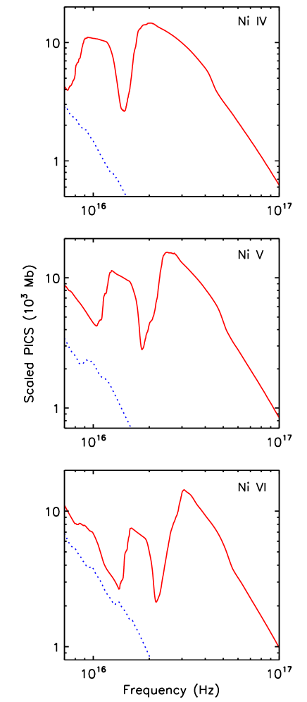
Figure 1: Plot of summed supercross-sections for Ni iv-vi calculated using autostructure (solid red) and a hydrogenic approximation (dotted blue). Prior to addition, each supercross-section was weight by a boltzmann factor and the statistical weight of the superlevel concerned.

As there are two different Ni line lists (Ku92 and Ku11), and two different sets of PICS (hydrogenic and those calculated with autostructure), there are four different combinations that we can test. Therefore, we calculated four different models in NLTE. We refer to these as Models 1, 2, 3, and 4. In Model 1, we use the Ku92 transitions and hydrogenic PICS. In Model 2, we use the Ku11 transitions and hydrogenic PICS. In Model 3, we use the Ku92 transitions and autostructure PICS. Finally, in Model 4, we use the Ku11 transitions and autostructure PICS. In all four cases, we based the models on a G191-B2B like atmosphere, and calculated the models with $T_{\mathrm{eff}}=52500$K, log $g=7.53$ (Barstow et al., 2003), and metal abundances listed in Table 5. These abundances were taken from Preval et al. (2013), measured in their analysis of the hot DA white dwarf G191-B2B. In the case where there was more than one ionization stage considered, we used the abundances with the smallest uncertainty. Listed in Table 6 are the model ions used in tlusty, along with the number of superlevels included.

Table 5: Metal abundances used in calculating the four model atmospheres described in text as a fraction of H. These abundances originate from Preval et al. (2013), where the values with the lowest statistical uncertainty were used.

Metal	Abundance X/H
He	$1.00\times{10}^{-5}$
C	$1.72\times{10}^{-7}$
N	$2.16\times{10}^{-7}$
O	$4.12\times{10}^{-7}$
Al	$1.60\times{10}^{-7}$
Si	$3.68\times{10}^{-7}$
P	$1.64\times{10}^{-8}$
S	$1.71\times{10}^{-7}$
Fe	$1.83\times{10}^{-6}$
Ni	$1.01\times{10}^{-6}$

Table 6: List of model ions and the number of levels used in model atmosphere calculations described in the text. Ions marked with * were treated approximately as single level ions by tlusty. For Ni, the number of levels outside and inside the brackets correspond to the number of levels for the Ku92 and Ku11 model ions, respectively.

Ion	Nsuperlevels
H i	9
H ii*	1
He i	24
He ii	20
He iii*	1
C iii	23
C iv	41
C v*	1
N iii	32
N iv	23
N v	16
N vi*	1
O iv	39
O v	40
O vi	20
O vii*	1
Al iii	23
Al iv*	1
Si iii	30
Si iv	23
Si v*	1
P iv	14
P v	17
P vi*	1
S iv	15
S v	12
S vi	16
S vii*	1
Fe iv	43
Fe v	42
Fe vi	32
Fe vii*	1
Ni iv	38 (73)
Ni v	48 (90)
Ni vi	42 (75)
Ni vii*	1

3.1 Spectral Energy Distribution

For this comparison, we considered the differences between the spectral energy distributions (SED) of each model. For each model, we synthesize three spectra covering the extreme ultraviolet (EUV), the ultraviolet (UV), and the optical regions. We then calculated the residual between models 1 and 2, 1 and 3, and 1 and 4 using the equation

$$\mathrm{Residual}=\frac{F_{\mathrm{i}}-F_{\mathrm{1}}}{F_{\mathrm{1}}},$$ (3)

where $F_{\mathrm{1}}$ is the flux for model 1, and $F_{\mathrm{i}}$ is the flux for model 2, 3, or 4.

3.2 Abundance variations

For this comparison, we wanted to examine the differences between abundances measured for G191-B2B when using each of the four models described above. Using a similar method to Preval et al. (2013), we measured the abundances for G191-B2B using all four of the models described above. The observational data for G191-B2B consists of three high S/N spectra constructed by co-adding multiple datasets. The first spectrum uses data from the Far Ultraviolet Spectroscopic Explorer (FUSE) spanning 910-1185Å, and the other two use data from the Space Telescope Imaging Spectrometer (STIS) aboard the Hubble Space Telescope (HST) spanning 1160-1680Å  and 1625-3145Å, respectively. A full list of the data sets used, and the coaddition procedure, is given in detail in Preval et al. (2013).

The model grids for each metal was constructed by using synspec. synspec takes a starting model converged assuming NLTE, and is able to calculate a spectrum for smaller or larger metal abundances by stepping away in LTE. We used the X-ray spectral package xspec (Arnaud, 1996) to measure the abundances. xspec takes a grid of models and observational data and interpolates between these models using a chi square ($\chi^{2}$) minimisation procedure. xspec is unable to use observational data with a large number of data points. To remedy this, we isolate individual absorption features for various ions and then use xspec to measure the abundances. A full list of the absorption features used and the sections of spectrum extracted is given in Table 9 in Preval et al. (2013). In addition to this list, we also include measurements of the O v abundance using the excited transition with wavelength 1371.296Å.

4 Results and discussion.

Here we discuss the results obtained from the four models calculated using permutations of the Ku92 and Ku11 atomic data, and the hydrogenic and autostructure cross-section data. Models 1, 2, 3, and 4 used Ku92/hydrogenic, Ku11/hydrogenic, Ku92/autostructure, and Ku11/autostructure respectively.

4.1 SED variations

In this subsection we discuss the differences between spectra synthesised for the four models described above.

4.1.1 EUV

Of all the spectral regions, the EUV undergoes the most dramatic changes. However, the EUV region appears to be relatively insensitive to whether Ku92 or Ku11 is used. In Figure 2 we have plotted the EUV region for models 1 and 2, along with the residual between these two models as defined in text. Below 200Å  the flux of model 2 appears to increase as wavelength decreases, being $\sim 15$% larger by 50Å. This may be due to how the superlevels are partitioned in the model calculation rather than a decrease in opacity from the Ku11 line list. In Figure 3 we plot the same region, but with models 1 and 3. Significant changes occur below 180Å, with the flux of model 3 being greatly attenuated, reaching a maximum of $\sim 80$% with respect to model 1. This is indicative of a larger opacity due to the autostructure PICS for Ni. Model 4 showed a combination of effects from models 2 and 3.

Figure 2: Plot of the EUV region covering 50-700Å  synthesised for models 1 (red solid) and 2 (blue dotted). On the bottom is a plot of the residual between the two models. The dashed line indicates a residual of zero, or no difference.

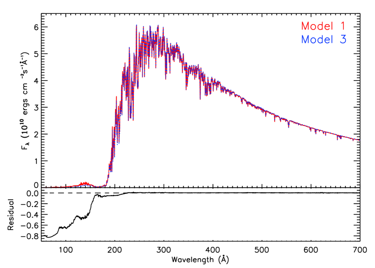
Figure 3: Same as Figure 2, but for models 1 and 3.

4.1.2 UV

In the case of the UV region, not a lot changes when using the autostructure PICS. In Figure 4 we have plotted synthetic spectra for Models 1 and 3 in the UV region. It can be seen that changes are limited to absorption features only, with the vast majority only changing depth by $\sim 3$%. The obvious exception to this is the N v doublet near 1240Å, where the depth has changed by $\sim 5-6$%. In Figure 5 we have now plotted models 1 and 2. Again, changes are limited to absorption features, but these are now far more pronounced, with depth changes of up to and beyond $10$%. These features can be attributed to Ni, and a few lighter metals, the abundances of which we discuss later. Again, Model 4 showed a combination of the changes seen in models 2 and 3.

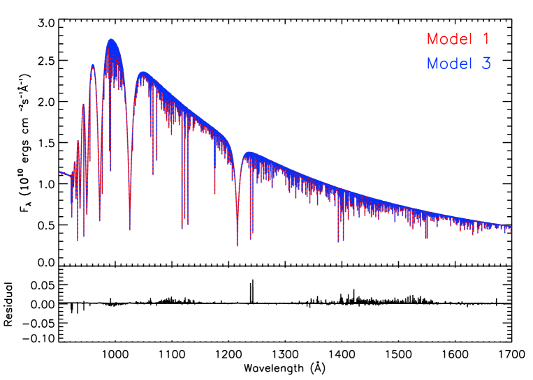
Figure 4: Plot of the UV region covering 910-1700Å  synthesised for models 1 (red solid) and 2 (blue dotted). On the bottom is a plot of the residual between the two models. The dashed line indicates a residual of zero, or no difference.

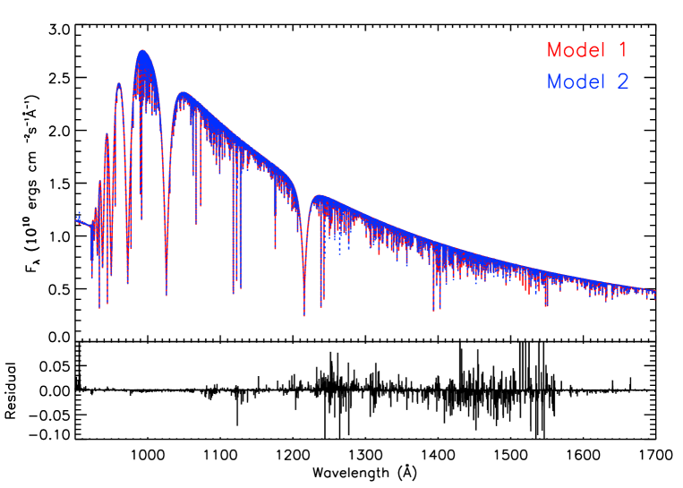
Figure 5: Same as Figure 4, but for models 1 (red solid) and 3 (blue dotted).

4.1.3 Optical

Very little to no change occurs in the optical region, regardless of line list or PICS used to calculate the models. In Figures 6 and 7 we plot the synthetic spectra of models 1 and 2, and 1 and 3 in the optical region respectively. In both cases, changes to both the continuum flux and H-balmer lines can be seen, but these are restricted to $<0.1$%. The same also occurs for model 4. Because these changes are so small, it is highly unlikely that measurements made using these models would be significantly different.

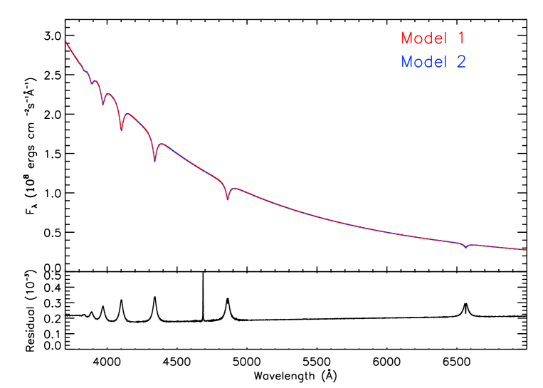
Figure 6: Plot of the optical region covering 3800-7000Å  synthesised for models 1 (red solid) and 2 (blue dotted). On the bottom is a plot of the residual between the two models. The sharp residual at  4690Å  is due to the He II 4860.677Å  transition.

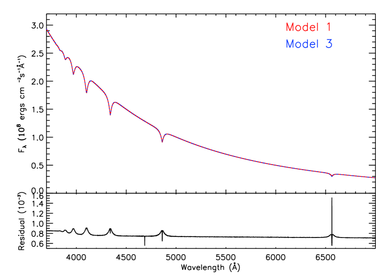
Figure 7: Same as Figure 6, but for models 1 (red solid) and 3 (blue dotted).

4.2 Abundance measurements

In Table 7 we list the abundance measurements made using the various models. We have also given the abundance differences between models 1 and 2, 1 and 3, and 1 and 4. Seven ions were found to have statistically significant abundance differences dependent on which model was used, namely N v, O iv, O v, Fe iv, Fe v, Ni iv, and Ni v.

4.2.1 N v

For N v, significant changes are seen in models 2, 3, and 4. Using model 1, we measured the abundance of N v to be $1.65^{+0.02}_{-0.02}\times{10}^{-7}$, whereas for models 2, 3, and 4, we find $1.77^{+0.02}_{-0.02}\times{10}^{-7}$, $1.87^{+0.02}_{-0.02}\times{10}^{-7}$, and $1.99^{+0.02}_{-0.02}\times{10}^{-7}$ respectively. The abundances measured using models 2, 3, and 4 correspond to increases from model 1 of $\sim 7$%, $\sim 13$%, and $\sim 20$% respectively. This suggests that both the number of transitions and the PICS used cause significant changes to the abundance.

4.2.2 O iv-v

In the case of O iv, significant changes in the abundances are seen when using the autostructure PICS in models 3 and 4. For O iv, we measured the abundance to be $4.63^{+0.12}_{-0.12}\times{10}^{-7}$ using model 1. For models 3 and 4, we measured abundances of $4.38^{+0.12}_{-0.12}\times{10}^{-7}$ and $4.31^{+0.12}_{-0.12}\times{10}^{-7}$ respectively, corresponding to decreases of $\sim 5$% and $\sim 7$% respectively.

A similar case occurs for O v, where statistically significant differences occur for models 3 and 4. Using model 1, we measured an abundance of $1.47^{+0.07}_{-0.07}\times{10}^{-6}$, whereas for models 3 and 4 we measured abundances of $1.69^{+0.08}_{-0.08}\times{10}^{-6}$ and $1.79^{+0.08}_{-0.08}\times{10}^{-6}$ respectively. This corresponds to an increase of $\sim 15$% and $\sim 22$% for models 3 and 4 over model 1 respectively. These results suggest that the largest changes to the O iv-v may be cause by the PICS rather than the number of transitions included in the line list.

4.2.3 Fe iv-v

The Fe iv-v abundances appear relatively insensitive to changes in the line list used and the PICS. A statistically significant difference was only observed between abundances measured using models 1 and 4. For Fe iv we measured an abundance of $2.05^{+0.04}_{-0.04}\times{10}^{-6}$ for model 1, and $1.98^{+0.04}_{-0.04}\times{10}^{-6}$ for model 4. This is a $\sim 3$% decrease from model 1. For Fe v, we measured abundances of $5.37^{+0.08}_{-0.08}\times{10}^{-6}$ and $5.20^{+0.07}_{-0.07}\times{10}^{-6}$ for models 1 and 4 respectively, corresponding to a $\sim 3$% decrease. These changes appear to suggest that a combination of both the number of transitions and PICS is required to change the abundance. We discuss this further below.

4.2.4 Ni iv-v

Interestingly, statistically significant changes compared to model 1 are seen in the Ni iv abundance when models 2 and 3 are used, but not for model 4. For model 1, we measured the abundance to be $3.00^{+0.09}_{-0.04}\times{10}^{-7}$. For models 2 and 3, we measure the abundances to be $2.81^{+0.05}_{-0.05}\times{10}^{-7}$ and $3.32^{+0.10}_{-0.10}\times{10}^{-7}$ respectively. This corresponds to a decrease of $\sim 6$% for model 2, and an increase of $\sim 11$% for model 3. In the case of model 4, an abundance of $2.97^{+0.12}_{-0.05}\times{10}^{-7}$ was measured.

The Ni v abundance appears to depend strongly upon whether Ku92 or Ku11 atomic data was included. In model 1, an abundance of $9.88^{+0.28}_{-0.21}\times{10}^{-7}$ was measured. For model 2, we measured the abundance to be $1.22^{+0.04}_{-0.04}\times{10}^{-6}$, being a $\sim 23$% increase from model 1. For model 3, only a very small difference was noted. We measured the abundance to be $9.81^{+0.23}_{-0.21}\times{10}^{-6}$, which is a $<1$% decrease. In model 4, we again see a large increase in the abundance from model 1, measuring $1.20^{+0.04}_{-0.04}\times{10}^{-6}$, which is a $\sim 21$% increase.

4.2.5 Ionization fraction agreement

In addition to the differences noted above, abundances for different ionization stages of N and O were found to diverge depending upon the PICS or atomic data used. In the case of N, the difference between the N iv and N v abundances for model 1 is $0.02^{+0.22}_{-0.22}\times{10}^{-7}$, whereas for models 2, 3, and 4 the differences are $-0.12^{+0.22}_{-0.22}\times{10}^{-7}$, $-0.25^{+0.22}_{-0.22}\times{10}^{-7}$, and $-0.39^{+0.22}_{-0.22}\times{10}^{-7}$ respectively. For O, the difference between the O iv and O v abundances for model 1 is $-1.01^{+0.07}_{-0.07}\times{10}^{-6}$, whereas for models 2, 3, and 4 the differences are $-1.11^{+0.07}_{-0.07}\times{10}^{-6}$, $-1.25^{+0.08}_{-0.08}\times{10}^{-6}$, and $-1.36^{+0.08}_{-0.08}\times{10}^{-6}$ respectively. The reason for this can be seen upon inspection of the ionization fractions for N and O. In Figures 8 and 9 we have plotted the ionization fractions for N and O against column mass for models 1 and 3. In both cases it can be seen that the model 3 ionization fractions have been shifted to smaller column masses. In the case of O, this effect is far more pronounced. In addition, it can also be seen that the shift to smaller column masses is larger for N/O v than it is for N/O iv. Therefore, this explains why the abundance measurements diverge.

Notwithstanding changes to the atomic data and PICS, the overall agreement between abundances measured for different ionization stages of particular species is generally poor. For this work, we adopted $T_{\mathrm{eff}}=52,500$K and log $g=7.53$ as measured by Barstow et al. (2003) for G191-B2B for models 1 to 4. These values were used for consistency with the work described by Preval et al. (2013). Since then, measurements of $T_{\mathrm{eff}}$ and log $g$ for G191-B2B have been revised upward by Rauch et al. (2013) to 60,000K and 7.60 respectively. The agreement between abundances measured for different ionization stages is a sensitive function of $T_{\mathrm{eff}}$, atmospheric composition, and to a lesser extent (sans H) log $g$. Our work was not focused on finding the best combination of $T_{\mathrm{eff}}$, log $g$, and atmospheric composition, but instead focused on whether a change, if any, occured to the measured abundances when altering the atomic data and PICS.

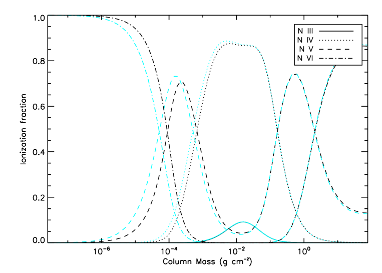
Figure 8: Plot of ionization fraction for N iv-vii for models 1 (black curve) and 3 (cyan curve). Colour figures are available online.

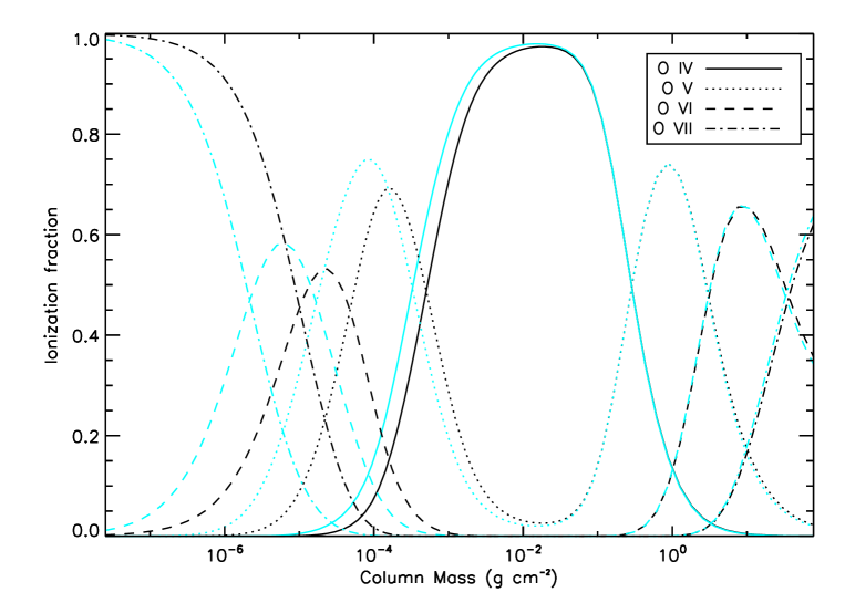
Figure 9: Same as Figure 8, but for O iv-vii.

4.2.6 Abundance differences

Interestingly, the difference between abundances measured using models 1 and 4 can be related to the differences between abundances measured using models 1 and 2, and 1 and 3. For example, the difference between the N v abundances measured using models 1 and 2 is $-0.12^{+0.02}_{-0.02}\times{10}^{-7}$, whereas for models 1 and 3, it is $-0.23^{+0.02}_{-0.02}\times{10}^{-7}$. If we add these differences from the abundance found in model 1, we obtain a total of $-0.35^{+0.03}_{-0.03}\times{10}^{-7}$. It is for this reason that we include an extra column in Table 7, where the differences between abundances measured using models 1 and 2, and 1 and 3, are summed together. It can be seen that in all cases, the sum of these is equal to (within the uncertainties) the 1-4 column. This is easily explained in terms of the opacity. Recall that the total opacity in a stellar atmosphere is just a linear sum of each individual contribution. In this case, it is the bound-free (PICS) and the bound-bound (Ku92 or Ku11) that is being added. Model 2 and Model 3 use the Ku11/Hydrogenic PICS and the Ku92/autostructure PICS respectively. Given that Model 1 uses the Ku92/Hydrogenic PICS, substracting the abundance found in Model 2 from Model 1 shows the effect of including more Ni transitions. Likewise, substracting the abundance found in Model 3 from Model 1 shows the effect of including more realistic PICS. Therefore, adding these two differences together will give the combination of these two effects. This explains why statistically significant differences were observed only when using model 4 for Fe iv-v, in that the effects of both the line list and the PICS combine.

Table 7: Summary of the abundances measured as a number fraction of H. The 1-2, 1-3, and 1-4 columns give the difference between abundances measured using these models. The $\Sigma$ column gives the sum of the 1-2 and 1-3 columns. Differences typeset in italics are statistically significant (i.e. consistent with a non-zero difference). Note $[x]=1\times{10}^{x}$

Ion	Model 1	Model 2	Model 3	Model 4	1 - 2	1 - 3	1 - 4	$\Sigma$
C iii	$1.83^{+0.03}_{-0.03}[-7]$	$1.83^{+0.03}_{-0.03}[-7]$	$1.83^{+0.03}_{-0.03}[-7]$	$1.83^{+0.03}_{-0.03}[-7]$	$0.00^{+0.04}_{-0.04}[-7]$	$0.00^{+0.04}_{-0.04}[-7]$	$0.00^{+0.04}_{-0.04}[-7]$	$0.00^{+0.06}_{-0.06}[-7]$
C iv	$3.00^{+0.10}_{-0.14}[-7]$	$3.00^{+0.10}_{-0.17}[-7]$	$3.00^{+0.10}_{-0.17}[-7]$	$3.00^{+0.09}_{-0.20}[-7]$	$0.00^{+0.14}_{-0.22}[-7]$	$0.00^{+0.15}_{-0.22}[-7]$	$0.00^{+0.14}_{-0.24}[-7]$	$0.00^{+0.21}_{-0.31}[-7]$
N iv	$1.67^{+0.22}_{-0.22}[-7]$	$1.65^{+0.22}_{-0.22}[-7]$	$1.62^{+0.22}_{-0.22}[-7]$	$1.60^{+0.22}_{-0.22}[-7]$	$0.02^{+0.31}_{-0.31}[-7]$	$0.05^{+0.31}_{-0.31}[-7]$	$0.07^{+0.31}_{-0.31}[-7]$	$0.07^{+0.44}_{-0.44}[-7]$
N v	$1.65^{+0.02}_{-0.02}[-7]$	$1.77^{+0.02}_{-0.02}[-7]$	$1.87^{+0.02}_{-0.02}[-7]$	$1.99^{+0.02}_{-0.02}[-7]$	$\mathit{-0.12^{+0.02}_{-0.02}[-7]}$	$\mathit{-0.23^{+0.02}_{-0.02}[-7]}$	$\mathit{-0.35^{+0.02}_{-0.02}[-7]}$	$-0.35^{+0.03}_{-0.03}[-7]$
O iv	$4.63^{+0.12}_{-0.12}[-7]$	$4.54^{+0.12}_{-0.12}[-7]$	$4.38^{+0.12}_{-0.12}[-7]$	$4.31^{+0.12}_{-0.12}[-7]$	$0.09^{+0.17}_{-0.17}[-7]$	$\mathit{0.25^{+0.17}_{-0.17}[-7]}$	$\mathit{0.32^{+0.17}_{-0.17}[-7]}$	$0.34^{+0.24}_{-0.24}[-7]$
O v	$1.47^{+0.07}_{-0.07}[-6]$	$1.56^{+0.07}_{-0.07}[-6]$	$1.69^{+0.08}_{-0.08}[-6]$	$1.79^{+0.08}_{-0.08}[-6]$	$-0.09^{+0.10}_{-0.10}[-6]$	$\mathit{-0.23^{+0.10}_{-0.10}[-6]}$	$\mathit{-0.32^{+0.11}_{-0.11}[-6]}$	$-0.32^{+0.14}_{-0.14}[-6]$
Al iii	$1.62^{+0.09}_{-0.09}[-7]$	$1.63^{+0.10}_{-0.10}[-7]$	$1.63^{+0.10}_{-0.10}[-7]$	$1.63^{+0.10}_{-0.10}[-7]$	$-0.01^{+0.13}_{-0.13}[-7]$	$-0.01^{+0.13}_{-0.13}[-7]$	$-0.01^{+0.13}_{-0.13}[-7]$	$-0.02^{+0.18}_{-0.18}[-7]$
Si iii	$2.90^{+0.39}_{-0.23}[-7]$	$2.89^{+0.38}_{-0.23}[-7]$	$2.92^{+0.41}_{-0.23}[-7]$	$2.92^{+0.41}_{-0.23}[-7]$	$0.00^{+0.54}_{-0.32}[-7]$	$-0.02^{+0.57}_{-0.33}[-7]$	$-0.02^{+0.56}_{-0.33}[-7]$	$-0.02^{+0.79}_{-0.46}[-7]$
Si iv	$3.32^{+0.20}_{-0.20}[-7]$	$3.33^{+0.20}_{-0.20}[-7]$	$3.34^{+0.20}_{-0.20}[-7]$	$3.35^{+0.20}_{-0.20}[-7]$	$-0.01^{+0.28}_{-0.28}[-7]$	$-0.02^{+0.28}_{-0.28}[-7]$	$-0.03^{+0.28}_{-0.28}[-7]$	$-0.03^{+0.40}_{-0.40}[-7]$
P iv	$1.34^{+0.20}_{-0.20}[-7]$	$1.34^{+0.20}_{-0.20}[-7]$	$1.30^{+0.19}_{-0.20}[-7]$	$1.30^{+0.19}_{-0.20}[-7]$	$0.00^{+0.28}_{-0.28}[-7]$	$0.03^{+0.28}_{-0.28}[-7]$	$0.04^{+0.28}_{-0.28}[-7]$	$0.03^{+0.40}_{-0.40}[-7]$
P v	$1.91^{+0.03}_{-0.03}[-8]$	$1.91^{+0.03}_{-0.03}[-8]$	$1.91^{+0.03}_{-0.03}[-8]$	$1.90^{+0.03}_{-0.03}[-8]$	$0.01^{+0.04}_{-0.04}[-8]$	$0.00^{+0.04}_{-0.04}[-8]$	$0.01^{+0.04}_{-0.04}[-8]$	$0.01^{+0.06}_{-0.06}[-8]$
S iv	$2.01^{+0.03}_{-0.03}[-7]$	$1.99^{+0.03}_{-0.03}[-7]$	$1.99^{+0.03}_{-0.03}[-7]$	$1.96^{+0.03}_{-0.03}[-7]$	$0.03^{+0.05}_{-0.05}[-7]$	$0.02^{+0.05}_{-0.05}[-7]$	$0.05^{+0.05}_{-0.05}[-7]$	$0.05^{+0.07}_{-0.07}[-7]$
S vi	$7.55^{+0.20}_{-0.20}[-8]$	$7.64^{+0.20}_{-0.20}[-8]$	$7.51^{+0.20}_{-0.20}[-8]$	$7.59^{+0.20}_{-0.20}[-8]$	$-0.08^{+0.28}_{-0.28}[-8]$	$0.05^{+0.28}_{-0.28}[-8]$	$-0.03^{+0.28}_{-0.28}[-8]$	$-0.03^{+0.40}_{-0.40}[-8]$
Fe iv	$2.05^{+0.04}_{-0.04}[-6]$	$2.01^{+0.04}_{-0.04}[-6]$	$2.02^{+0.04}_{-0.04}[-6]$	$1.98^{+0.04}_{-0.04}[-6]$	$0.04^{+0.05}_{-0.05}[-6]$	$0.03^{+0.05}_{-0.05}[-6]$	$\mathit{0.07^{+0.05}_{-0.05}[-6]}$	$0.07^{+0.07}_{-0.07}[-6]$
Fe v	$5.37^{+0.08}_{-0.08}[-6]$	$5.31^{+0.07}_{-0.07}[-6]$	$5.27^{+0.07}_{-0.07}[-6]$	$5.20^{+0.07}_{-0.07}[-6]$	$0.06^{+0.11}_{-0.11}[-6]$	$0.10^{+0.11}_{-0.11}[-6]$	$\mathit{0.17^{+0.11}_{-0.11}[-6]}$	$0.16^{+0.16}_{-0.16}[-6]$
Ni iv	$3.00^{+0.09}_{-0.04}[-7]$	$2.81^{+0.05}_{-0.05}[-7]$	$3.32^{+0.10}_{-0.10}[-7]$	$2.97^{+0.12}_{-0.05}[-7]$	$\mathit{0.19^{+0.10}_{-0.06}[-7]}$	$\mathit{-0.32^{+0.13}_{-0.10}[-7]}$	$0.03^{+0.15}_{-0.07}[-7]$	$-0.13^{+0.16}_{-0.12}[-7]$
Ni v	$9.88^{+0.28}_{-0.21}[-7]$	$1.22^{+0.04}_{-0.04}[-6]$	$9.81^{+0.23}_{-0.21}[-7]$	$1.20^{+0.04}_{-0.04}[-6]$	$\mathit{-2.30^{+0.29}_{-0.22}[-7]}$	$0.06^{+0.37}_{-0.30}[-7]$	$\mathit{-2.12^{+0.29}_{-0.22}[-7]}$	$-2.24^{+0.47}_{-0.37}[-7]$

4.3 General discussion

Ideally, any calculation should be as accurate as possible including the most up-to-date data available. However, this also needs to be balanced in terms of time constraints, and the task at hand. We have seen that in the EUV, the choice of using either Ku92 or Ku11 is irrelevant as the change is very small. The shape of the continuum, however, is very sensitive to the PICS used. The downside to using the larger line list from Ku11 increases the calculation time significantly. For example, Model 1 took $\sim 17500$ seconds (292 minutes) to converge, whereas Model 2 took $\sim 37000$ seconds (617 minutes). This is because the Ku11 data has more energy levels, and is hence split into a larger number of superlevels than for Ku92 data.

From a wider perspective, the PICS calculated using autostructure caused the most changes, in that the EUV continuum was severly attenuated, and abundances for N and O were changed. When using the Ku11 line list in model atmospheres, abundances for Ni changed significantly while the continua for various spectral regions were left relatively unchanged. Given that a calculation with Ku11 data takes twice as long to do than with Ku92, an abundance change in only Ni iv-v is relatively little payoff compared to the physics we can learn from changing the PICS. The way forward in improving the quality of future model atmosphere calculations is clear; effort should be focused on improving the PICS data for ions where it exists, as well as filling in gaps where it is required (in this case, for Ni).

This piece of work has been a proof-of-concept endeavour. While we have shown that replacing hydrogenic cross-section data with more realistic calculations has a significant effect on synthesised spectra and measurements, we have only considered direct PI. If a direct PI-only calculation has this large an effect, then it stands to reason that a full calculation including photoexcitation/autoionization resonances will cause a greater effect.

The applications of this work is not limited to white dwarf stars. This data can be used in stellar atmosphere models for objects of any kind, and any temperature range. We chose to demonstrate the effects of our calculations on a hot DA white dwarf star as calculations for these objects are relatively simple. At this temperature regime, we do not need to worry about the effects of 3D modelling, convection etc.

4.4 Future work

As mentioned in our discussion, this work has been a proof-of-concept. The next step is to extend our PICS calculations to include other ions of Ni. Once this is done, we plan to include the omitted resonances to our calculations, and re-examine the effect including this data has on model spectra and measurements.

The present PICS data was calculated using a distorted wave approximation. A potentially more accurate calculation can be achieved using the R-matrix method as in the Opacity Project. Therefore, we aim to do some test calculations to compare Ni PICS using both the R-matrix or distorted wave approximation.

The EUV spectra of hot metal polluted white dwarfs has historically been difficult to model (cf. Lanz et al. 1996; Barstow et al. 1998), the key to which may be the input atomic physics. Therefore, we will also consider the quality of fits to the EUV spectra of several metal polluted white dwarf stars.

5 Conclusion

We have presented our PICS calculations of Ni iv-vi using the distorted wave code autostructure. We investigated the effect of using two different line lists (Ku92 and Ku11) and two different sets of PICS (hydrogenic and autostructure) on synthesized spectra and abundance measurements based on the hot DA white dwarf G191-B2B. This investigation was done by calculating four models (labelled 1, 2, 3, and 4) with permutations of the Ni line list and PICS used. Model 1 used Ku92 line list/hydrogenic PICS, Model 2 used Ku11 line list/hydrogenic PICS, Model 1 used Ku92 line list/autostructure PICS, and model 4 used Ku11 line list/autostructure PICS.

We synthesised model spectra for each of the four models in the EUV, UV, and optical regions. In the EUV, model 3 showed large attentuation shortward of 180Å  of up to $\sim 80$% relative to model 1, whereas model 2 was relatively unchanged. In the UV, the continuum was unchanged in models 2 and 3. However, in model 2, the Ni absorption feature depths changed significant, increasing in depth by up to $\sim 10$%. Absorption features in model 3 were relatively unchanged, with depth changes of $\sim 3$% across the spectrum. In the optical, changes in flux were so small ($<0.1$%) across models that these are unlikely to be observed, nor would it be possible to differentiate between them. Model 4 was not plotted in the EUV, UV, or optical as the resultant spectrum was just a combination of the effects observed in models 2 and 3.

We measured metal abundances for G191-B2B using all four models. This was to see if there were any differences in the metal abundances measured when changing the PICS or atomic data included in the model calculation. Statistically significant (consistent with non-zero difference compared to model 1) abundance changes were observed in N v over all models, and O iv-v when using models 3 and 4. This suggests that the N abundances are sensitive to both the line list and PICS used, while the O abundances were only sensitive to the PICS. The Fe iv-v abundances only changed by a statistically significant amount for model 4, implying a combination of the line list and cross-section caused the change. The Ni iv-v abundances changed by a statistically significant amount for models 2 and 4, implying the line list caused the difference. Interestingly, for each metal abundance, the difference between measurements made using models 1 and 4 could be found by summing the differences between measurements made using models 1 and 2, and models 1 and 3. This is in keeping with the assumption that predicted radiation for small variations of the opacity sources scales roughly linearly with the opacity.

In addition, we found the abundances of N/O iv and v diverged depending on the PICS used. A comparison of the ionization fractions calculated using models 1 and 3 showed that the charge states for model 3 formed higher in the atmosphere than the charge states for model 1. Furthermore, N/O v experiences a larger change with respect to depth formation than N/O iv, explaining the divergence of the abundance measurements.

Our work has demonstrated that, even with a limited calculation, the Ni PICS have made a significant difference to the synthetic spectra, and by extension what is measured from observational data. Comparatively, an extended line list such as Ku11 offers little benefit given the extended computational time required to converge a model atmosphere, and the small pay off (changed Ni abundance). It is our opinion that future atomic data calculations for stellar atmosphere models should not necessarily focus on how big the line list is, but the quality of the PICS.

References

- Anderson (1989) Anderson L. S., 1989, ApJ, 339, 558
- Arnaud (1996) Arnaud K. A., 1996, in Jacoby G. H., Barnes J., eds, Astronomical Data Analysis Software and Systems V Vol. 101 of Astronomical Society of the Pacific Conference Series, XSPEC: The First Ten Years. p. 17
- Badnell (1986) Badnell N. R., 1986, J. Phys. B, 19, 3827
- Badnell (1997) Badnell N. R., 1997, J. Phys. B, 30, 1
- Badnell (2011) Badnell N. R., 2011, Comput. Phys. Commun., 182, 1528
- Barstow et al. (2003) Barstow M. A., Good S. A., Holberg J. B., Hubeny I., Bannister N. P., Bruhweiler F. C., Burleigh M. R., Napiwotzki R., 2003, MNRAS, 341, 870
- Barstow et al. (1998) Barstow M. A., Hubeny I., Holberg J. B., 1998, MNRAS, 299, 520
- Chayer et al. (1995) Chayer P., Fontaine G., Wesemael F., 1995, ApJS, 99, 189
- Cowan (1981) Cowan R. D., 1981, The Theory of Atomic Structure and Spectra. Los Alamos Series in Basic and Applied Sciences, University of California Press
- Eissner & Nussbaumer (1969) Eissner W., Nussbaumer H., 1969, J. Phys. B, 2, 1028
- Holberg et al. (1994) Holberg J. B., Hubeny I., Barstow M. A., Lanz T., Sion E. M., Tweedy R. W., 1994, ApJL, 425, L105
- Hubeny (1988) Hubeny I., 1988, Comput. Phys. Commun., 52, 103
- Hubeny & Lanz (1995) Hubeny I., Lanz T., 1995, ApJ, 439, 875
- Hubeny & Lanz (2011) Hubeny I., Lanz T., 2011, in Astrophysics Source Code Library, record ascl:1109.022 Synspec: General Spectrum Synthesis Program. p. 9022
- Kurucz (1992) Kurucz R. L., 1992, RMxAA, 23, 45
- Kurucz (2011) Kurucz R. L., 2011, Canadian Journal of Physics, 89, 417
- Lanz et al. (1996) Lanz T., Barstow M. A., Hubeny I., Holberg J. B., 1996, ApJ, 473, 1089
- Preval et al. (2013) Preval S. P., Barstow M. A., Holberg J. B., Dickinson N. J., 2013, MNRAS, 436, 659
- Rauch et al. (2013) Rauch T., Werner K., Bohlin R., Kruk J. W., 2013, A&A, 560
- Seaton & Badnell (2004) Seaton M. J., Badnell N. R., 2004, MNRAS, 354, 457
- Vennes & Lanz (2001) Vennes S., Lanz T., 2001, ApJ, 553, 399
- Werner & Dreizler (1994) Werner K., Dreizler S., 1994, AAP, 286, L31