Auxiliary gradient-based sampling algorithms

Abstract

We introduce a new family of MCMC samplers that combine auxiliary variables, Gibbs sampling and Taylor expansions of the target density. Our approach permits the marginalisation over the auxiliary variables yielding marginal samplers, or the augmentation of the auxiliary variables, yielding auxiliary samplers. The well-known Metropolis-adjusted Langevin algorithm (MALA) and preconditioned Crank-Nicolson Langevin (pCNL) algorithm are shown to be special cases. We prove that marginal samplers are superior in terms of asymptotic variance and demonstrate cases where they are slower in computing time compared to auxiliary samplers. In the context of latent Gaussian models we propose new auxiliary and marginal samplers whose implementation requires a single tuning parameter, which can be found automatically during the transient phase. Extensive experimentation shows that the increase in efficiency (measured as effective sample size per unit of computing time) relative to (optimised implementations of) pCNL, elliptical slice sampling and MALA ranges from 10-fold in binary classification problems to 25-fold in log-Gaussian Cox processes to 100-fold in Gaussian process regression, and it is on par with Riemann manifold Hamiltonian Monte Carlo in an example where the latter has the same complexity as the aforementioned algorithms. We explain this remarkable improvement in terms of the way alternative samplers try to approximate the eigenvalues of the target. We introduce a novel MCMC sampling scheme for hyperparameter learning that builds upon the auxiliary samplers. The MATLAB code for reproducing the experiments in the article is publicly available and a Supplement to this article contains additional experiments and implementation details.

1 Introduction

Monte Carlo sampling is the preferable tool for uncertainty quantification and statistical learning in a wide range of scientific problems. We are interested in Bayesian learning problems where the density to be sampled is proporional to $\pi_{0}(\mathbf{x}|\boldsymbol{\theta})\exp\{f(\mathbf{x})\}$, where $\pi_{0}(\mathbf{x}|\boldsymbol{\theta})$ is the prior, potentially depending on hyperparameters $\boldsymbol{\theta}$, and $f(\mathbf{x})$ is the log-likelihood; the dependence on any data is suppressed throughout; we highlight the dependence on $\boldsymbol{\theta}$ when it is part of the inference and wish to sample from $\pi(\mathbf{x},\boldsymbol{\theta})\propto\pi_{0}(\mathbf{x}|\boldsymbol{\theta})\exp\{f(\mathbf{x})\}p(\boldsymbol{\theta})$ where $p(\boldsymbol{\theta})$ is a prior on the hyperparameters; when the hyperparameters are fixed we might drop them from the notation and write $\pi_{0}(\mathbf{x})$ instead. Whereas the main algorithmic construction and some theory is generic, the field of application in this article and all the experiments refer to latent Gaussian models where $\pi_{0}(\mathbf{x}|\boldsymbol{\theta})=\mathcal{N}(\mathbf{x}|\bm{0},\mathbf{C})$.

Major challenges with MCMC in these contexts are: (i) Likelihood-informed proposals; gradient-based methods based on discretisations of the Langevin diffusion, e.g. the preconditioned Metropolis-adjusted Langevin algorithm (pMALA) of mala and the manifold MALA (mMALA) of Girolami11 are typical examples. (ii) Prior-informed proposals, i.e., ones that are in agreement with the dependence structure imposed by the prior; this is particularly important for priors that impose smoothness and create strong dependencies among the components of $\mathbf{x}$, e.g. Gaussian priors; neal first proposed such a sampler which has evolved to the elliptical slice sampler of murrayEllipt , and has been extended to the preconditioned Crank-Nicolson (pCN) samplers of .beskos:2008:bridges+methods+diffusion who show that failure to be prior-informed leads to collapse of algorithms in high-dimensional problems that can otherwise be avoided. The preconditioned Crank-Nicolson Langevin samplers of Cotter2013MCMC , are likelihood and prior informed. (iii) Numerically efficient computation of the accept-reject mechanism within Metropolis-Hastings schemes, which can be the bottleneck for scaling up MCMC to big data problems, see e.g. teh , ericLang , arnak .(iv) The numerically efficient generation of proposals; see e.g. davies .

We introduce a new family of MCMC samplers that are both prior and likelihood informed and are constructed using a combination of auxiliary variables and Taylor expansions. The essence of the approach is to use the proposals used within standard MCMC as auxiliary variables and sample the augmented target using Metropolis-within-Gibbs. The resultant algorithms are called auxiliary samplers and the algorithm that is obtained by integrating the auxiliary variables out is called a marginal sampler. We prove that the marginal sampler is better in Peskun ordering than its corresponding auxiliary sampler. We apply the construction in latent Gaussian models and introduce three new MCMC samplers for such models, two auxiliary and one marginal; one of the auxiliary samplers for latent Gaussian models (the scheme based on the auxiliary variable $\mathbf{z}$ as detailed in Section 3.3) was first sketched in a discussion in (Titsias2011, ). We show that pCNL is a special case of the new framework. We carry out an extensive series of experiments where we compare our new samplers with pCN, elliptical slice sampler (Ellipt), pMALA, pCNL. The implementation of all these algorithms involves an $\mathcal{O}(n^{2})$ cost per iteration, where $n$ is the dimension of $\mathbf{x}$, and requires a single tuning parameter. For log-Gaussian Cox processes we also compare against mMALA and the Riemann manifold Hamiltonian Monte Carlo (RMHMC) of Girolami11 , since in this context these can also be implemented at an $\mathcal{O}(n^{2})$ cost, whereas their implementation is typically $\mathcal{O}(n^{3})$. We demonstrate that our new samplers are more efficient in terms of effective sample size per unit of computing time than pMALA, pCN, Ellipt and pCNL by a factor that ranges from 10 to 100 in standard machine learning and spatial statistics problems, and are comparable to RMHMC when the latter can also be implemented at $\mathcal{O}(n^{2})$ cost. We provide an explanation on why these gains are achieved in terms of the way the different algorithms approximate the spectrum of the target by shrinking differently the eigenvalues of the prior covariance.

One of the proposed auxiliary samplers has smaller computational time than the marginal sampler since it involves a smaller number of matrix-vector multiplications; actually its acceptance probability can be computed an order of magnitude faster than that of the marginal sampler. Nevertheless, all the experiments reported here and in a Supplement find the marginal sampler superior to the auxiliary ones even when computing cost is taken into account. We also investigate empirically the optimal tuning of the new algorithms and find the auxiliary ones to require tuning around 50% acceptance rate and the marginal around 60%. Utilising one of the auxiliary samplers, we propose a novel sampler for $\pi(\mathbf{x},\boldsymbol{\theta})\propto\mathcal{N}(\mathbf{x};\bm{0},\mathbf{C}_{\boldsymbol{\theta}})\exp\{f(\mathbf{x})\}p(\boldsymbol{\theta})$ where $\boldsymbol{\theta}$ are hyperparameters. We find impressive efficiency gains relative to alternative samplers in the context of multi-class Gaussian process classification.

The paper is organised as follows. Section 2 introduces auxiliary and marginal samplers and proves a comparison result. Section 3 develops the methodology for latent Gaussian models. Section 4 introduces a sampler for joint inference of the latent Gaussian process and its hyperparameters. Section 5 contains an extensive series of numerical experiments. A Supplement to this article contains additional theoretical results, implementation details, pseudocode of the proposed algorithms, and several simulation experiments. All experiments are completely reproducible and the code can be found in https://github.com/mtitsias/aGrad.

2 Auxiliary versus marginal samplers

We start with a generic result about the use of auxiliary variables within Metropolis-Hastings schemes. This result establishes that the marginal samplers we introduce in this article are statistically more efficient than the auxiliary samplers we also introduce; statistical efficiency here is measured by the asymptotic variance of ergodic averages computed using the samples generated by the algorithms, hence the averages computed using marginal samplers are shown to have lower asymptotic variance than those using auxiliary samplers. However, we will later establish concrete situations where the auxiliary samplers are computationally more efficient, in particular the use of auxiliary variables can change the complexity of the computation of the Metropolis-Hastings ratio. Hence, our broader framework allows for the exchange of statistical with computational efficiency for better scalability of the algorithms.

2.1 Auxiliary Metropolis-Hastings samplers

Consider a target density $\pi(\mathbf{x})$ and a hierarchical mechanism for generating proposals $\mathbf{y}$ within a Metropolis-Hastings sampler for probing $\pi(\mathbf{x})$, by first drawing $\mathbf{u}\sim q(\mathbf{u}|\mathbf{x})$ and then $\mathbf{y}\sim q(\mathbf{y}|\mathbf{x},\mathbf{u})$. Hence, the overall proposal density is

$$q(\mathbf{y}|\mathbf{x})=\int q(\mathbf{y}|\mathbf{x},\mathbf{u})q(\mathbf{u}|\mathbf{x})\mathrm{d}\mathbf{u}\,.$$

What we will call a marginal scheme proposes in this way and accepts with probability the minimum of 1 and the Metropolis-Hastings ratio,

$${\pi(\mathbf{y})q(\mathbf{x}|\mathbf{y})\over\pi(\mathbf{x})q(\mathbf{y}|\mathbf{x})}\,.$$

However, we can alternatively augment the state-space with $\mathbf{u}$ as an auxiliary variable and design a sampler for $\pi(\mathbf{x},\mathbf{u})=\pi(\mathbf{x})q(\mathbf{u}|\mathbf{x})$. We can sample from this extended target by Hastings-within-Gibbs:

1. Sample $\mathbf{u}|\mathbf{x}\sim\pi(\mathbf{u}|\mathbf{x})=q(\mathbf{u}|\mathbf{x})$

2. Propose $\mathbf{y}|\mathbf{u},\mathbf{x}\sim q(\mathbf{y}|\mathbf{x},\mathbf{u})$ and accept the move with probability

   $$1\wedge{\pi(\mathbf{y}|\mathbf{u})q(\mathbf{x}|\mathbf{y},\mathbf{u})\over\pi(\mathbf{x}|\mathbf{u})q(\mathbf{y}|\mathbf{x},\mathbf{u})}\,.$$

Hence, a Metropolis-Hastings step is used to sample the intractable $\pi(\mathbf{x}|\mathbf{u})$. Let us call this second scheme an auxiliary sampler. In this formulation, the marginal and auxiliary samplers use the same ingredients, $q(\mathbf{u}|\mathbf{x})$ and $q(\mathbf{y}|\mathbf{x},\mathbf{u})$, and marginally generate the same proposals $\mathbf{y}$ from a given state $\mathbf{x}$. However, their acceptance mechanisms differ.

2.2 An example: auxiliary MALA

We start with a random walk proposal, $\mathcal{N}(\mathbf{u}|\mathbf{x},(\delta/2)\mathbf{I})$ to define an augmented target

$$\pi(\mathbf{x},\mathbf{u})\propto\pi(\mathbf{x})q(\mathbf{u}|\mathbf{x})=\pi(\mathbf{x})\mathcal{N}(\mathbf{u}|\mathbf{x},(\delta/2)\mathbf{I})$$

and sample from this using an auxiliary sampler, as described above. In order to sample the intractable $\pi(\mathbf{x}|\mathbf{u})$ we do a first order approximation to the log target density, around $\mathbf{x}$, given by $\log\pi(\mathbf{y})\approx\log\pi(\mathbf{x})+\nabla\log\pi(\mathbf{x})^{T}(\mathbf{y}-\mathbf{x})$, and combine it with $q(\mathbf{u}|\mathbf{y})$ to obtain the proposal

$$q(\mathbf{y}|\mathbf{u},\mathbf{x}) \propto\exp\{\log\pi(\mathbf{x})+\nabla\log\pi(\mathbf{x})^{T}(\mathbf{y}-\mathbf{x})\}\mathcal{N}(\mathbf{u}|\mathbf{y},(\delta/2)\mathbf{I})$$

$$\propto\mathcal{N}(\mathbf{y}|\mathbf{u}+(\delta/2)\nabla\log\pi(\mathbf{x}),(\delta/2)\mathbf{I})\,.$$

The corresponding marginal sampler is the Metropolis-adjusted Langevin algorithm (MALA) since $q(\mathbf{y}|\mathbf{x})=\mathcal{N}(\mathbf{y}|\mathbf{x}+(\delta/2)\nabla\log\pi(\mathbf{x}),\delta\mathbf{I})$.

2.3 Marginal samplers are Peskun better than auxiliary samplers

Recall that a Markov transition kernel $P_{2}$ dominates in Peskun ordering another $P_{1}$ if $P_{1}(\mathbf{x},A)\leq P_{2}(\mathbf{x},A)$ for all measurable $A$ such that $\mathbf{x}\notin A$, and for all $\mathbf{x}$. An important implication of this ordering is that if $P_{1}$ and $P_{2}$ are ergodic kernels and the corresponding ergodic averages admit a central limit theorem for a given function, then the asymptotic variance of those averages for the function are larger for $P_{1}$ relative to $P_{2}$. This comparison was introduced in peskun , extended in tierney and then in leisen .

Proposition 1.

The marginal sampler is better in Peskun ordering than the auxiliary sampler.

This result can be proved by noting that the auxiliary sampler we consider is a special case of the framework described in Proposition 2 of storvik ; the general framework in storvik considers samplers where two auxiliary variables are used, but the use of a single auxiliary variable is more appropriate for the specific samplers we introduce in Section 3 for latent Gaussian models. Note also a recent result in the literature on so-called pseudomarginal methods, where auxiliary variables are used to provide unbiased estimators of $\pi(\mathbf{x})$ when this is intractable or expensive to compute. Theorem 7 of andrieu-pm establishes that the corresponding auxiliary sampler is less statistically efficient (in the sense described above) than the marginal sampler. andrieu-pm also consider alternative auxiliary variable schemes.

3 Gradient-based samplers for latent Gaussian models

3.1 Setting and objectives

We now focus on the latent Gaussian models where the target density is written in the form

$$\pi(\mathbf{x})\propto\exp\{f(\mathbf{x})\}\mathcal{N}(\mathbf{x}|\bm{0},\mathbf{C}),$$ (1)

where $\exp\{f(\mathbf{x})\}$ is the likelihood and $\mathcal{N}(\mathbf{x}|\bm{0},\mathbf{C})$ is the Gaussian prior which for simplicity we assume to have zero mean. We are interested in general-purpose, black-box algorithms that would perform reasonably well in a wide range of applications. With respect to the dimension of the target, $n$, the algorithms we consider can be implemented (including the transient phase where step sizes are tuned) at $\mathcal{O}(n^{2})$ cost, given an initial $\mathcal{O}(n^{3})$ offline pre-computation, provided that $f(\mathbf{x})$ and $\nabla f(\mathbf{x})$ are computed at $\mathcal{O}(n^{2})$ cost. It is practically important that no matrix decompositions are needed even for the transient phase of the algorithms where algorithmic parameters, such as step size, are tuned to achieve theoretically-motivated optimal acceptance rates. It is also practically important that algorithms use a small number of tuning parameters, and all the algorithms we consider here use a single one. We make no assumptions about special properties of $\mathbf{C}$, such as Toeplitz or banded. Section 5 contains several model structures that fit into this category and range from multi-class classification to point processes. A Supplement includes details on optimal implementation and details on the computational cost of each algorithm.

3.2 Review of popular MCMC samplers for latent Gaussian models

Here, we summarise the main popular MCMC samplers used in the context of latent Gaussian models. The most basic gradient-based approach is the preconditioned MALA (pMALA) that generates proposals according to

$$q(\mathbf{y}|\mathbf{x})=\mathcal{N}(\mathbf{y}|\mathbf{x}+\frac{\delta}{2}\mathbf{\Sigma}\nabla\log\pi(\mathbf{x}),\delta\mathbf{\Sigma}),$$

where $\mathbf{\Sigma}$ is a preconditioning matrix and $\delta$ is a step size parameter that has to be tuned. This proposal is obtained as a first-order Euler discretization of the Langevin stochastic differential equation (SDE),

$$\mathrm{d}\mathbf{X}_{t}={1\over 2}\mathbf{\Sigma}\nabla\log\pi(\mathbf{X}_{t})\mathrm{d}t+\mathbf{\Sigma}^{1/2}\mathrm{d}\mathbf{W}_{t},$$

where $\mathbf{W}$ is Brownian motion, which is a stochastic process reversible with respect to $\pi(\mathbf{x})$. For good sampling we might prefer to choose the preconditioning in a state-dependent way to capture the local covariance structure. This is for example the idea behind certain schemes used in Girolami11 that are referred there as simplified manifold MALA (mMALA) proposals. However, such algorithms would require matrix decompositions at each iteration. For latent Gaussian models the common state-independent choice is $\mathbf{\Sigma}=\mathbf{C}$, while often the choice $\mathbf{\Sigma}=\mathbf{I}$ doesn’t work at all since it ignores the correlation structure introduced by the Gaussian prior. Hence, in this paper we only consider pMALA with $\mathbf{\Sigma}=\mathbf{C}$, which leads to the proposal

$$q(\mathbf{y}|\mathbf{x}) =\mathcal{N}\left(\mathbf{y}|(1-\frac{\delta}{2})\mathbf{x}+\frac{\delta}{2}\mathbf{C}\nabla f(\mathbf{x}),\delta\mathbf{C}\right)\,.$$

The generation of proposals cost is $\mathcal{O}(n^{2})$, including the initial tuning of the algorithm for choosing a $\delta$ that yields approximately 50% acceptance probability following scaleSS . The Metropolis-Hastings ratio, which involves the Gaussian prior, requires an $\mathcal{O}(n^{2})$ computing cost.

Cotter2013MCMC review proposals based on more advanced Crank-Nicolson discretisations of the Langevin SDE, and focus on the so-called Crank-Nicolson Langevin (CNL) proposal

$$q(\mathbf{y}|\mathbf{x}) =\mathcal{N}(\mathbf{y}|(2\mathbf{C}+\delta\mathbf{I})^{-1}(2\mathbf{C}-\delta\mathbf{I})\mathbf{x}+2\delta(2\mathbf{C}+\delta\mathbf{I})^{-1}\mathbf{C}\nabla f(\mathbf{x}),$$

$$8\delta(2\mathbf{C}+\delta\mathbf{I})^{-1}\mathbf{C}(2\mathbf{C}+\delta\mathbf{I})^{-1})$$

and the preconditioned Crank-Nicolson Langevin (pCNL) proposal

$$q(\mathbf{y}|\mathbf{x})=\mathcal{N}\left(\mathbf{y}|{2\over 2+\delta}\mathbf{x}+{\delta\over 2+\delta}\mathbf{C}\nabla f(\mathbf{x}),{\delta(\delta+4)\over(2+\delta)^{2}}\mathbf{C}\right).$$ (2)

We have parameterised pCNL so that its step size $\delta$ is comparable to that in the samplers we introduce in this article, hence the discrepancy with the notation used in Cotter2013MCMC . We consider only pCNL in this paper since it has been found to be more efficient in practice. The Metropolis-Hastings ratio for pCNL becomes

$$\exp\{f(\mathbf{y})-f(\mathbf{x})+k(\mathbf{x},\mathbf{y})-k(\mathbf{y},\mathbf{x})\}$$ (3)

where

$$k(\mathbf{x},\mathbf{y})={2+\delta\over 4+\delta}\mathbf{x}^{T}\nabla f(\mathbf{y})-{\delta\over 2(\delta+4)}\nabla f(\mathbf{y})^{T}\mathbf{C}\nabla f(\mathbf{y})\,.$$

Note that the prior density is cancelled in the ratio, which is a consequence of a reversibility property this proposal mechanism enjoys and is discussed in Section 3.4. Notice also that the mean of the pMALA proposal is essentially the same as the the mean of pCNL since both can be re-written in the form $\beta\mathbf{x}+(1-\beta)\mathbf{C}\nabla f(\mathbf{x})$ where $\beta\in[0,1]$. Note that for this reparametrization to hold the step $\delta$ for pMALA must be in the range $[0,1/2]$. The generation of proposals and the computation of the Metropolis-Hastings ratio require an $\mathcal{O}(n^{2})$ cost. When the gradient term is dropped we obtain the Crank-Nicolson and the preconditioned Crank-Nicolson (pCN) algorithms, which are only prior informed. The more interesting pCN corresponds to the proposal

$$q(\mathbf{y}|\mathbf{x})=\mathcal{N}\left(\mathbf{y}|{2\over 2+\delta}\mathbf{x},{\delta(\delta+4)\over(2+\delta)^{2}}\mathbf{C}\right)$$ (4)

and it was originally proposed by neal and more recently in a function space context by .beskos:2008:bridges+methods+diffusion . Section 3.4 discusses that pCN proposal is reversible with respect to the prior, which leads to an appealing simplification of the Metropolis-Hastings ratio that becomes simply $\exp\{f(\mathbf{y})-f(\mathbf{x})\}$. Therefore, pCN involves a $\mathcal{O}(n^{2})$ cost for generating proposals but only an $\mathcal{O}(n)$ for deciding on their acceptance.

Finally, in this article we consider the elliptical slice sampler (Ellipt) proposed by (murrayEllipt, ), which is popular in the machine learning community. This scheme combines the pCN proposal with a slice sampling procedure that is constrained on an ellipse that avoids rejections, hence its proposal mechanism does not have any step sizes that need tuning. However, the rejection-free property comes with the cost that multiple log-likelihood evaluations are required per iteration.

3.3 New auxiliary and marginal samplers

The starting point of an auxiliary sampler is the augmentation with the auxiliary variable $\mathbf{u}$ drawn from $q(\mathbf{u}|\mathbf{x})=\mathcal{N}(\mathbf{u}|\mathbf{x},(\delta/2)\mathbf{I})$ so that

$$\pi(\mathbf{x},\mathbf{u})\propto\exp\{f(\mathbf{x})\}\mathcal{N}(\mathbf{x}|\bm{0},\mathbf{C})\mathcal{N}(\mathbf{u}|\mathbf{x},(\delta/2)\mathbf{I}).$$

The auxiliary sampler requires an approximation to $\pi(\mathbf{x}|\mathbf{u})$ to be used as a proposal. Since the product $\mathcal{N}(\mathbf{x}|\bm{0},\mathbf{C})\mathcal{N}(\mathbf{u}|\mathbf{x},(\delta/2)\mathbf{I})$, yields a Gaussian density for $\mathbf{x}$, we do a first order Taylor expansion of $f(\mathbf{x})$ around the current value $\mathbf{x}$ to come up with a Gaussian proposal density that is both prior and likelihood informed:

$$q(\mathbf{y}|\mathbf{x},\mathbf{u})\propto \exp\{f(\mathbf{x})+\nabla f(\mathbf{x})^{T}(\mathbf{y}-\mathbf{x})\}\mathcal{N}(\mathbf{y}|\bm{0},\mathbf{C})\mathcal{N}(\mathbf{u}|\mathbf{y},(\delta/2)\mathbf{I})$$

$$\propto\mathcal{N}\left(\mathbf{y}|\frac{2}{\delta}\mathbf{A}(\mathbf{u}+{\delta\over 2}\nabla f(\mathbf{x})),\mathbf{A}\right),$$

where

$$\mathbf{A}=(\mathbf{C}^{-1}+{2\over\delta}\mathbf{I})^{-1}={\delta\over 2}(\mathbf{C}+{\delta\over 2}\mathbf{I})^{-1}\mathbf{C}.$$ (5)

$\mathbf{A}$ can be defined in any of the alternative ways, which are of course equivalent when $\mathbf{C}$ is invertible. However, $\mathbf{A}$ can be defined as the second expression when $\mathbf{C}$ is not invertible (in which case the first expression is invalid). The second expression is also computationally preferrable when $\mathbf{C}$ is close to being singular. Thus, the auxiliary sampler iterates:

1. $\mathbf{u}\sim\mathcal{N}\left(\mathbf{u}|\mathbf{x},(\delta/2)\mathbf{I}\right)$

2. Propose $\mathbf{y}\sim q(\mathbf{y}|\mathbf{x},\mathbf{u})$ and accept it according to the Metropolis-Hastings ratio

   $$\exp\left\{f(\mathbf{y})-f(\mathbf{x})+j(\mathbf{x},\mathbf{y},\mathbf{u})-j(\mathbf{y},\mathbf{x},\mathbf{u})\right\},$$ (6)

   $$j(\mathbf{x},\mathbf{y},\mathbf{u})=\left(\mathbf{x}-\frac{2}{\delta}\mathbf{A}(\mathbf{u}+{\delta\over 4}\nabla f(\mathbf{y}))\right)^{T}\nabla f(\mathbf{y})\,.$$ (7)

The matrix $\mathbf{A}$ involved in the algorithm has the same eigenspace as $\mathbf{C}$. Hence, given a spectral decomposition of $\mathbf{C}$ at the onset, generating from the proposal $q(\mathbf{y}|\mathbf{u},\mathbf{x})$ has computational cost $\mathcal{O}(n^{2})$. Also, the Metropolis-Hastings ratio has cost $\mathcal{O}(n^{2})$.

The corresponding marginal scheme is obtained by simply marginalising out the auxiliary variable $\mathbf{u}$ to obtain the marginal proposal

$$q(\mathbf{y}|\mathbf{x}) =\int\mathcal{N}(\mathbf{y}|{2\over\delta}\mathbf{A}(\mathbf{u}+(\delta/2)\nabla f(\mathbf{x})),\mathbf{A})\mathcal{N}\left(\mathbf{u}|\mathbf{x},(\delta/2)\mathbf{I}\right)d\mathbf{u}$$

$$=\mathcal{N}\left(\mathbf{y}|{2\over\delta}\mathbf{A}\left(\mathbf{x}+{\delta\over 2}\nabla f(\mathbf{x})\right),{2\over\delta}\mathbf{A}^{2}+\mathbf{A}\right)\,,$$

where we have used that $\mathbf{A}$ is symmetric. One way to generate from the proposal $q(\mathbf{y}|\mathbf{x})$ is to be based on the mixture representation above, which corresponds to the same two-step procedure used in the auxiliary scheme and it has computational cost $\mathcal{O}(n^{2})$. The corresponding Metropolis-Hastings ratio simplifies to

$$\exp\{f(\mathbf{y})-f(\mathbf{x})+h(\mathbf{x},\mathbf{y})-h(\mathbf{y},\mathbf{x})\},$$

$$h(\mathbf{x},\mathbf{y})=\left(\mathbf{x}-\frac{2}{\delta}\mathbf{A}(\mathbf{y}+{\delta\over 4}\nabla f(\mathbf{y}))\right)^{T}\left({2\over\delta}\mathbf{A}+\mathbf{I}\right)^{-1}\nabla f(\mathbf{y})\,$$

and it is also computed at an $\mathcal{O}(n^{2})$ cost.

A reparameterization of the auxiliary variable $\mathbf{u}$ yields an alternative auxiliary sampler in this context, that corresponds to the same marginal sampler. We define a new auxiliary variable $\mathbf{z}$

$$\mathbf{z}\equiv\mathbf{u}+(\delta/2)\nabla f(\mathbf{x})\sim\mathcal{N}(\mathbf{z}|\mathbf{x}+(\delta/2)\nabla f(\mathbf{x}),(\delta/2)\mathbf{I}),$$

so that the initial proposal distribution $q(\mathbf{y}|\mathbf{x},\mathbf{u})$ in the former auxiliary sampler now becomes $q(\mathbf{y}|\mathbf{z})=\mathcal{N}\left(\mathbf{y}|(2/\delta)\mathbf{A}\mathbf{z},\mathbf{A}\right)$. This has the interesting property that the proposed $\mathbf{y}$ becomes conditionally independent from the current $\mathbf{x}$ given the auxiliary variable $\mathbf{z}$; we explicitly exploit this when we design samplers for learning hyperparameters in Section 4. Subsequently, with this formulation, we can work with an alternative expanded target,

$$\pi(\mathbf{x},\mathbf{z})\propto\exp\{f(\mathbf{x})\}\mathcal{N}(\mathbf{x}|\bm{0},\mathbf{C})\mathcal{N}(\mathbf{z}|\mathbf{x}+(\delta/2)\nabla f(\mathbf{x}),(\delta/2)\mathbf{I})\,,$$

and consider an auxiliary sampler that iterates between the steps:

1. $\mathbf{z}\sim\mathcal{N}\left(\mathbf{z}|\mathbf{x}+(\delta/2)\nabla f(\mathbf{x}),(\delta/2)\mathbf{I}\right)$

2. Propose $\mathbf{y}\sim q(\mathbf{y}|\mathbf{z})$ and accept it according to the Metropolis-Hastings ratio

   $$\exp\left\{f(\mathbf{y})-f(\mathbf{x})+g(\mathbf{z},\mathbf{y})-g(\mathbf{z},\mathbf{x})\right\},$$

   $$g(\mathbf{z},\mathbf{y})=\left(\mathbf{z}-\mathbf{y}-(\delta/4)\nabla f(\mathbf{y})\right)^{T}\nabla f(\mathbf{y})\,.$$

The simplification in the acceptance ratio follows by noting that

$$\mathcal{N}\left(\mathbf{y}|\frac{2}{\delta}\mathbf{A}\mathbf{z},\mathbf{A}\right)\propto\mathcal{N}(\mathbf{y}|\bm{0},\mathbf{C})\mathcal{N}(\mathbf{z}|\mathbf{y},(\delta/2)\mathbf{I})\,.$$

The first step of the algorithm is likelihood-informed while the second step is prior-informed and these two-types of information are linked by the auxiliary variable $\mathbf{z}$. The marginal sampler that corresponds to this scheme is precisely the one obtained earlier. However, the Metropolis-Hastings ratio is computable at $\mathcal{O}(n)$ cost when $f(\mathbf{x})$ and $\nabla f(\mathbf{x})$ are also computable at $\mathcal{O}(n)$ cost. This is in contrast with the marginal sampler and the auxiliary sampler based on $\mathbf{u}$. Thus, the auxiliary sampler based on $\mathbf{z}$ allows a tradeoff between computational and statistical efficiency.

3.4 Connection to Crank-Nicolson schemes and a covariance shrinkage perspective on algorithmic performance

We can easily construct preconditioned auxiliary and marginal samplers by taking $q(\mathbf{u}|\mathbf{x})=\mathcal{N}(\mathbf{u}|\mathbf{x},(\delta/2)\mathbf{\Sigma})$. The corresponding marginal proposal is

$$q(\mathbf{y}|\mathbf{x}) =\mathcal{N}\left(\mathbf{y}|{2\over\delta}\mathbf{B}\mathbf{\Sigma}^{-1}\left(\mathbf{x}+{\delta\over 2}\mathbf{\Sigma}\nabla f(\mathbf{x})\right),{2\over\delta}\mathbf{B}\mathbf{\Sigma}^{-1}\mathbf{B}+\mathbf{B}\right)\,,$$ (8)

where $\mathbf{B}=(\frac{2}{\delta}\mathbf{\Sigma}^{-1}+\mathbf{C}^{-1})^{-1}$. Now if we set $\mathbf{\Sigma}=\mathbf{C}$ this proposal becomes that of pCNL (2) in Section 3.2. Interestingly, it can be checked that for no choice of $\mathbf{\Sigma}$ CNL is a special case of the marginal sampler. The experiments in Section 5 demonstrate that the marginal sampler leads to a significant increase in efficiency, that can be as large as 100-fold over pCNL. Here we provide some insights on the success of the marginal algorithm and some further connections to recent algorithms that have been devised to improve upon pCN.

We first observe that when $\nabla f=\bm{0}$, the marginal sampler proposal density is reversible with respect to the prior. This follows from the Lemma below, the proof of which is given in a Supplement to this article. Notice that part (a) is stated in terms of laws without assuming the existence of Lebesgue densities, to even cover cases where the prior covariance is singular; in practice it is also interesting to have proposal mechanisms that do not require inversion of $\mathbf{C}$, which even when invertible might be very ill-conditioned for smooth latent Gaussian processes.

Lemma 1.

1. Suppose that $\mathbf{F}$ is symmetric and commutes with $\mathbf{C}$. Then, the transition kernel $\mathcal{N}(\mathrm{d}\mathbf{y}|\mathbf{F}\mathbf{x},(\mathbf{I}-\mathbf{F}^{2})\mathbf{C})$ is reversible with respect to the prior $\mathcal{N}(\mathrm{d}\mathbf{x}|\bm{0},\mathbf{C})$.

2. Suppose that $\mathbf{C}$ is invertible with $\mathbf{C}=\bm{\Gamma}^{2}$ and $\mathbf{F}$ is symmetric. Then the transition density $\mathcal{N}(\mathbf{y}|\bm{\Gamma}\mathbf{F}\bm{\Gamma}^{-1}\mathbf{x},\bm{\Gamma}(\mathbf{I}-\mathbf{F}^{2})\bm{\Gamma})$ is reversible with respect to $\mathcal{N}(\mathbf{x}|\bm{0},\mathbf{C})$.

The choice $\mathbf{F}=\{2/(2+\delta)\}\mathbf{I}$ in Lemma 1 (a) yields pCN; the choice $\mathbf{F}=\{\mathbf{C}+(\delta/2)\mathbf{I}\}^{-1}\mathbf{C}=(2/\delta)\mathbf{A}$ yields the marginal sampler proposal when $\nabla f=\bm{0}$, see a Supplement to this article for the calculations that establish this correspondence. Therefore, one perspective on the proposed marginal sampler is as a principled extension of pCNL that changes the preconditioning matrix from a multiple of identity to one informed by $\mathbf{C}$ while requiring a single tuning parameter $\delta$. This perspective links the marginal sampler to some recent work in the inverse problem literature that improves upon pCN, such as kody1 ; kody2 , which we review below.

The proposal covariances used in the marginal sampler and pCNL have the same eigenvectors as that of $\mathbf{C}$, but they have different eigenvalues. In particular, an eigenvalue $\gamma$ of $\mathbf{C}$ is mapped to

$$p(\gamma)=\left(1-{4\over(\delta+2)^{2}}\right)\gamma\quad\mbox{and}\quad m(\gamma)={\delta(\delta+4\gamma)\over(\delta+2\gamma)^{2}}\gamma$$

in pCNL and the marginal samplers respectively, where $\delta$ is the step size used in each algorithm. Whereas pCNL shrinks multiplicatively all eigenvalues of $\mathbf{C}$ by the same factor, the marginal sampler shrinks adaptively with the interesting property that $m^{\prime}(0)=1$, hence small eigenvalues are left practically unchanged, and $m(\gamma)\to\delta$ as $\gamma\to\infty$. Suppose now that the latent Gaussian field is observed with additive Gaussian error with variance $\sigma^{2}$, as in the experiments of Section 5.1. Then, the posterior covariance has the same eigenvectors as $\mathbf{C}$ but an eigenvalue $\gamma$ of $\mathbf{C}$ is mapped to $t(\gamma)=\gamma\sigma^{2}/(\gamma+\sigma^{2})$. Hence, the posterior is shrunk a lot where the prior is weak, with $\gamma\gg\sigma^{2}$ mapped to approximately $\sigma^{2}$, but $\gamma\ll\sigma^{2}$ being left practically unchanged. In fact, by taking $\delta=\sigma^{2}$, we get that $m(\gamma)/t(\gamma)$ ranges from 1 to approximately 1.12 for the whole range of possible $\gamma,\sigma^{2}$ values. Thus, we should expect the marginal sampler when tuned to achieve a good acceptance probability (which we empirically have found to be between 50-60%, see Section 5) to choose a $\delta$ close to $\sigma^{2}$ and by doing so, to capture the appropriate range of values for all eigenvalues of the target covariance; this is corroborated by the experiments of Section 5. On the other hand, pCNL needs to set $\delta$ as approximately $\sigma^{2}/\gamma$ in order to match a specific eigenvalue $\gamma$; the experiments of Section 5 show that when tuned optimally pCNL chooses a step size which is $\sigma^{2}/\gamma_{\max}$, where $\gamma_{\max}$ is the largest eigenvalue of $\mathbf{C}$, which is of course the one that has experienced the largest change relative to the prior; however, this step size is too small for the modes of the system for which the posterior is similar to the prior, hence the posterior distribution of those is explored poorly.

An intuition along the above lines for the weakness of pCN proposal to capture the spectrum of the posterior is developed in Section 3 of kody1 in the context of Bayesian inverse problems, which points out that better algorithms should shrink by different amounts different eigenvalues. Such algorithms were originally proposed in kody1 and then explored much more thoroughly in kody2 ; these works explore the framework of Lemma 1 (b) and work with autoregressive matrices $\mathbf{F}$ different from multiples of the identity. The construction requires that $\mathbf{C}$ is invertible and a transformation of the latent field to standard Gaussian (or white noise when working with infinite-dimensional Gaussians). Then, $\mathbf{F}$ is such that in directions of the posterior strongly informed by the likelihood a different step size is used than in those where the prior dominates. This machinery requires a preliminary exploration of the posterior to estimate a matrix the eigendecomposition of which, together with some eigenvalue thresholding, determine the so-called likelihood informed subspace, i.e., those directions where the likelihood dominates, and its complement. The resultant algorithms involve a large number of tuning parameters and although the authors have made a serious effort to automatize their choice, they are not "plug-and-play" in the way that all other algorithms we have mentioned so far are. This is why we do not consider them further in this article.

4 Hyperparameter learning for latent Gaussian models

An important issue in latent Gaussian models is concerned with the inference over hyperparameters of the covariance matrix $\mathbf{C}$, hence we need to design MCMC samplers that sample also from the corresponding posterior distribution of those, together with the latent field. This problem is challenging because of the high dependence between these hyperparameters and the state vector $\mathbf{x}$. To deal with this, several approaches have been presented in the literature KnorrHeld02 ; ncp ; murrayCovhyper ; FilipponeML13 ; hensman2015mcmc ; sahu . Next, we discuss a new sampling move tailored to the auxiliary sampler based on the latent variable $\mathbf{z}$. This is basically a proof of concept implementation. Let $\boldsymbol{\theta}$ denote the hyperparameters of the covariance, $\mathbf{C}_{\boldsymbol{\theta}}$, and $p(\boldsymbol{\theta})$ their prior density. In the rest of this section we index matrices that depend on the unknown hyperparameters $\boldsymbol{\theta}$, to emphasise the dependence and the fact that they would have to be updated whenever $\boldsymbol{\theta}$ changes during sampling. We consider the expanded target

$$\pi(\mathbf{x},\mathbf{z},\boldsymbol{\theta})\propto\exp\{f(\mathbf{x})\}\mathcal{N}(\mathbf{x}|\bm{0},\mathbf{C}_{\boldsymbol{\theta}})\mathcal{N}(\mathbf{z}|\mathbf{x}+(\delta/2)\nabla f(\mathbf{x}),(\delta/2)\mathbf{I})p(\boldsymbol{\theta})\,.$$

To deal with the dependence between $\boldsymbol{\theta}$ and $\mathbf{x}$, we construct a joint move $(\mathbf{x},\boldsymbol{\theta})\rightarrow(\mathbf{y},\boldsymbol{\theta}^{\prime})$, conditional on the auxiliary variable $\mathbf{z}$, with proposal

$$q(\mathbf{y},\boldsymbol{\theta}^{\prime}|\mathbf{x},\boldsymbol{\theta},\mathbf{z})=q(\mathbf{y}|\boldsymbol{\theta}^{\prime},\mathbf{z})q(\boldsymbol{\theta}^{\prime}|\boldsymbol{\theta}),$$

where

$$q(\mathbf{y}|\boldsymbol{\theta}^{\prime},\mathbf{z})=\mathcal{N}(\mathbf{y}|\frac{2}{\delta}\mathbf{A}_{\boldsymbol{\theta}^{\prime}}\mathbf{z},\mathbf{A}_{\boldsymbol{\theta}^{\prime}})=\frac{1}{\mathcal{Z}(\mathbf{z},\boldsymbol{\theta}^{\prime})}\mathcal{N}(\mathbf{y}|\bm{0},\mathbf{C}_{\boldsymbol{\theta}^{\prime}})\mathcal{N}(\mathbf{z}|\mathbf{y},(\delta/2)\mathbf{I}).$$

Here, $\mathbf{A}_{\boldsymbol{\theta}}=(\mathbf{C}_{\boldsymbol{\theta}}^{-1}+(2/\delta)\mathbf{I})^{-1}$ while $\mathcal{Z}(\mathbf{z},\boldsymbol{\theta}^{\prime})=\mathcal{N}(\mathbf{z}|\bm{0},\mathbf{C}_{\boldsymbol{\theta}^{\prime}}+(\delta/2)\mathbf{I})$ is a marginal likelihood term. The corresponding Metropolis-Hastings acceptance ratio simplifies to

$$\exp\left\{f(\mathbf{y})-f(\mathbf{x})+g(\mathbf{z},\mathbf{y})-g(\mathbf{z},\mathbf{x})\right\}\times\frac{\mathcal{Z}(\mathbf{z},\boldsymbol{\theta}^{\prime})p(\boldsymbol{\theta}^{\prime})q(\boldsymbol{\theta}|\boldsymbol{\theta}^{\prime})}{\mathcal{Z}(\mathbf{z},\boldsymbol{\theta})p(\boldsymbol{\theta})q(\boldsymbol{\theta}^{\prime}|\boldsymbol{\theta})}\,.$$

This ratio has an interesting product form. The first term, corresponding to $\exp\left\{f(\mathbf{y})-f(\mathbf{x})+g(\mathbf{z},\mathbf{y})-g(\mathbf{z},\mathbf{x})\right\}$, comes from the auxiliary sampler and does not depend on $\boldsymbol{\theta}$. In contrast the second term does not depend on $\mathbf{x}$ and is a Metropolis-Hastings ratio for targeting the posterior on $\boldsymbol{\theta}$ that would arise if the observations were $\mathbf{z}$ and were generated as a noisy observation of the latent field, having isotropic Gaussian noise with variance $\delta/2$. Due to this noise, the conditional density proportional to $\mathcal{N}(\mathbf{z}|\bm{0},\mathbf{C}_{\boldsymbol{\theta}}+(\delta/2)\mathbf{I})p(\boldsymbol{\theta})$ will be flatter than the one that arises when we do Gibbs sampling on $\pi(\mathbf{x},\boldsymbol{\theta})$, i.e., $\mathcal{N}(\mathbf{x}|\bm{0},\mathbf{C}_{\boldsymbol{\theta}})p(\boldsymbol{\theta})$, hence we expect to get better mixing. Notice also that it is possible to generalize the above move so that the proposal on the hyperparameters becomes dependent on the auxiliary variable $\mathbf{z}$, i.e. to take the form $q(\boldsymbol{\theta}^{\prime}|\boldsymbol{\theta},\mathbf{z})$. This, for instance, could allow to use a standard MALA proposal to target $\mathcal{Z}(\mathbf{z},\boldsymbol{\theta})p(\boldsymbol{\theta})$.

The above move shares some similarities with the approach in murrayCovhyper who also use auxiliary variables to inflate the covariance $\mathbf{C}_{\boldsymbol{\theta}}$ with an isotropic or diagonal covariance. However, the two main differences with that work is that our approach is likelihood-informed through the re-sampling step of the auxiliary variable $\mathbf{z}\sim\mathcal{N}(\mathbf{z}|\mathbf{x}+(\delta/2)\nabla f(\mathbf{x}),(\delta/2)\mathbf{I})$ which depends on $\nabla f(\mathbf{x})$, and is based on joint sampling as opposed to a reparametrization.

The update of $\boldsymbol{\theta}$ necessitates the decomposition of $\mathbf{C}_{\boldsymbol{\theta}}$ and requires an $\mathcal{O}(n^{3})$ computation. Therefore, every such update is expensive. To compensate for that we can do many latent process updates for each $\boldsymbol{\theta}$ update.

5 Experiments

We test the proposed samplers in several latent Gaussian models applied to simulated and real data. The purpose of the experiments is to investigate the performance of the three proposed samplers detailed in Section 3: i) the marginal sampler (mGrad), ii) the sampler based on auxiliary variable $\mathbf{u}$ (aGrad-u) and iii) the sampler based on $\mathbf{z}$ (aGrad-z). Recall, that all three algorithms generate the same proposals but are based on different rules for their acceptance. The three new schemes are compared against the methods reviewed earlier in Section 3.2: pMALA, pCN, pCNL, Ellipt. All algorithms have been implemented in MATLAB in an unified and highly optimized code outlined in a Supplement and available online. In one examples we also use mMALA and RMHMC based on the code provided by the authors (Girolami11, ), since their implementation in this setting can also be done at $\mathcal{O}(n^{2})$ cost. In all the experiments the step size of pCN was tuned to achieve acceptance rate in the range $20\%$ to $30\%$, while for all the remaining algorithms that use gradient information from the likelihood the step size was tuned to achieve an acceptance rate in the range $50\%$ to $60\%$. This adaptation phase takes place only during burn-in iterations, while at collection of samples stage the step size is kept fixed. Notice that Ellipt does not require tuning a step size since it accepts all samples. The pilot tuning of $\delta$ can be done in a computationally efficient way for all algorithms, see a Supplement to this article for details. See the Supplement also for more figures, experiments and details.

5.1 Gaussian process regression and small noise limit

The aim of this experiment is to compare the methods under different levels of the likelihood informativeness. For simplicity, we shall consider a simple Gaussian process regression setting where the likelihood is Gaussian so that

$$f(\mathbf{x})=-\frac{n}{2}\log(2\pi\sigma^{2})-\frac{1}{2\sigma^{2}}\sum_{i=1}^{n}(y_{i}-x_{i})^{2}$$ (9)

and where each $y_{i}$ is a scalar real-valued observation. We take the prior covariance matrix $\mathbf{C}$ to be defined via the squared exponential kernel function $c(\mathbf{s}_{i},\mathbf{s}_{j})=\sigma_{x}^{2}\exp\{-\frac{1}{2\ell^{2}}||\mathbf{s}_{i}-\mathbf{s}_{j}||^{2}\}$ where $\mathbf{s}_{i}$ is a input vector associated with the latent function value $x_{i}$. Under the above model, the informativeness of the likelihood depends on the noise variance $\sigma^{2}$. We generated three regression datasets having $n=1000$ and noise variances $\sigma^{2}=1,0.1\ \text{and}\ 0.01$. Autocorrelation summaries of MCMC output are plotted in Figure 3. Autocorrelation lines are plotted against CPU running time and they have been averaged over ten repeats (using different random seeds) of the experiments, where the CPU time has incorporated the burn-in iterations that are then removed for estimating the autocorrelations.

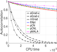
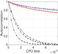
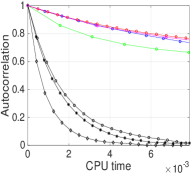
Figure 1: Estimated autocorrelation of the function $f(\mathbf{x})$ for all algorithms against CPU time; the lines are averages over ten runs of the algorithms.

Note that in the limit $\sigma^{2}\to 0$ the prior and the posterior are mutually singular, hence prior-informed only proposals will collapse. For each experiment the noise variance $\sigma^{2}$ was kept fixed to its ground-truth value that generated the data and the covariance matrix $\mathbf{C}$ was also fixed and precomputed using suitable values of the kernel hyperparameters $(\sigma_{x}^{2},\ell^{2})$. To infer the $1000$-dimensional vector $\mathbf{x}$ we run all alternative sampling schemes for $10^{4}$ burn-in iterations (starting from a state vector $\mathbf{x}$ equal to zero) and then we collected $5\times 10^{3}$ samples. For the third dataset where $\sigma^{2}=0.01$, pCN, pCNL, Ellipt, and pMALA converge more slowly and therefore we had to increase the number of burn-in iterations to $3\times 10^{4}$. Table 1 provide quantitative results such as effective sample size (ESS), running times and an overall efficiency score for the very challenging case where $\sigma^{2}=0.01$; the Supplement contains such results for the other two simulations. The overall efficiency, given by the last column of the Tables labelled as Min ESS/s, is described as the ratio between minimum ESS (among all dimensions of $\mathbf{x}$) over running time. Regarding the performance of the three new samplers we can observe the following. Firstly, all samplers converge very fast in all cases and generate highly effective mixing chains with large effective sample sizes (ESS). The highest ESS is always achieved by mGrad, followed by aGrad-u and aGrad-z. However, if we also take into account computational time, the aGrad-z scheme becomes more competitive and it can outperform aGrad-u. Secondly, both speed of convergence and sampling performance remains stable as the informativeness of the likelihood increases. This is achieved through learning the step size $\delta$ which adapts to the noise of the likelihood - see the argumentation in Section 3.4. Remarkably, in all cases for mGrad $\delta$ tends to be slightly larger than $\sigma^{2}$, while for aGrad-u and aGrad-z $\delta$ is smaller (about a half) than $\sigma^{2}$. Regarding the other methods, their performance (see Min ESS/s) is at least one order of magnitude worse than aGrad-z. Notice the step size $\delta$ learned pCN, pCNL and pMALA is not within the same range of the noise variance $\sigma^{2}$, but instead it is much smaller - it is actually about $\sigma^{2}/\gamma_{\max}$ where $\gamma_{\max}$ is the largest eigenvalue of $\mathbf{C}$, as predicted by the arguments in Section 3.4.

Table 1: Comparison of sampling methods in the regression dataset with $\sigma^{2}=0.01$. All numbers are averages across ten repeats where also one-standard deviation is given for the Min ESS/s score.

Method Time(s) Step $\delta$ ESS (Min, Med, Max) Min ESS/s (s.d.) aGrad-z 5.5 0.005 (306.7, 430.9, 539.3) 55.48 (5.96) aGrad-u 6.9 0.006 (345.8, 459.3, 584.8) 50.27 (4.02) mGrad 5.8 0.011 (856.0, 1095.6, 1301.1) 147.67 (9.97) pMALA 49.3 < 0.001 (8.4, 45.1, 155.5) 0.17 (0.07) Ellipt 11.0 (12.9, 50.3, 144.8) 1.18 (0.34) pCN 6.6 < 0.001 (8.0, 35.4, 107.7) 1.21 (0.42) pCNL 23.9 < 0.001 (8.7, 54.4, 208.6) 0.36 (0.13)

5.2 Log-Gaussian Cox Process

We consider a log-Gaussian Cox model and apply the sampling schemes to the same model and dataset used in (Girolami11, ). We also consider a down-sampled version of this dataset in order to investigate how the methods behave under mesh refinement. More precisely, we assume that an area of interest $[0,1]^{2}$ is discretized into a $64\times 64$ regular grid, and each latent variable $x_{ij}$ is associated with the grid cell $(i,j),i,j,=1,\ldots,64$. The dimension of $\mathbf{x}$ is $n=4096$. We assume that a data vector of counts is generated independently given a latent intensity process $\lambda(\cdot)$ so that each $y_{ij}$ is Poisson distributed with mean $\lambda_{ij}=m\exp(x_{ij}+v)$, where $m=1/4096$ is the area of the grid cell and $v$ is a constant mean value. The $4096$-dimensional latent vector $\mathbf{x}$ is drawn from a Gaussian process with zero-mean and covariance function

$$k((i,j),(i^{\prime},j^{\prime}))=\sigma_{x}^{2}\exp(-\sqrt{(i-i^{\prime})^{2}+(j-j^{\prime})^{2}}/64\beta)\,.$$

The likelihood is Poisson form, hence

$$f(\mathbf{x})=\sum_{i,j}^{64}\left(y_{ij}(x_{ij}+v)-m\exp(x_{ij}+v)\right)\,.$$

We used the dataset from (Girolami11, ) that was simulated by the above model by setting the hyperparameters to $\beta=1/33$, $\sigma_{x}^{2}=1.91$ and $v=\log(126)-\sigma_{x}^{2}/2$. The objective was to infer the latent vector $\mathbf{x}$ while keeping the hyperparameters $(\beta,\sigma^{2},v)$ fixed to their ground truth values. Following the experimental protocol in (Girolami11, ) we run the algorithms for $2000$ burn-in iterations and then we collected $5000$ posterior samples. Furthermore, for this experiment we also included in the comparison the two main algorithms in (Girolami11, ) namely the manifold MALA (mMALA) and the Riemann Manifold Hamiltonian Monte Carlo (RMHMC) by using the software provided by the authors. Table 2 provides quantitative scores (see the Supplement to this article for some trace plots). We can observe that the new samplers have significantly better performance than all competitors but RMHMC. The latter has slightly less Min ESS/s than mGrad. However, notice that for this log-Gaussian Cox model, and due to the analytic properties of the log-likelihood, RMHMC and mMALA use a constant metric tensor (i.e. the preconditioning matrix $\mathbf{\Sigma}$) that does not depend on $\mathbf{x}$ (Girolami11, ). This is an ideal scenario for RMHMC and mMALA which allows the computational cost to be $O(n^{2})$, i.e. the same cost as for all other methods in Table 2. For more complex models the metric tensor will depend on $\mathbf{x}$, which makes RMHMC and mMALA extremely slow due to the $O(n^{3})$ computational cost per sampling iteration. As in the previous experiment in terms of ESS mGrad is best followed by aGrad-u and then aGrad-z, although in terms of ESS per unit of time the fastest aGrad-z scheme gets closer to aGrad-u. Also, notice again the striking pattern of the learned step sizes for the new samplers (third column in Table 2) that positively correlate with ESS. In the Supplement we show an experiment with down-sampled sparser $32\times 32$ grid; results show that $\delta$ in the proposed gradient samplers is found to be 4 times smaller than on the finer grid, reflecting the larger information of the data per latent variable in the sparser dataset. The sampling efficiency of the proposed algorithms remains unchanged under mesh coarseness, only computing times decrease.

Table 2: Comparison of sampling methods in the log-Gaussian Cox model dataset in the original version where $n=4096$. All numbers are averages across ten repeats where also one-standard deviation is given for the Min ESS/s score.

Method Time(s) Step $\delta$ ESS (Min, Med, Max) Min ESS/s (s.d.) aGrad-z 89.6 0.962 (36.1, 181.2, 507.5) 0.40 (0.10) aGrad-u 134.6 2.814 (95.8, 469.3, 1092.4) 0.71 (0.14) mGrad 132.0 5.887 (177.8, 801.1, 1628.6) 1.35 (0.15) pMALA 218.7 0.006 (3.5, 12.9, 59.3) 0.02 (0.00) Ellipt 51.5 (4.2, 17.0, 66.0) 0.08 (0.01) pCN 47.4 0.012 (3.3, 12.0, 57.6) 0.07 (0.00) pCNL 87.7 0.006 (3.4, 12.6, 60.2) 0.04 (0.00) mMALA 334.1 0.070 (21.4, 84.7, 179.4) 0.06 (0.02) RHMC 1493.7 0.100 (1825.7, 4452.2, 5000.0) 1.22 (0.09)

5.3 Binary Gaussian process classification

In this section we consider binary Gaussian process classification where given a set of training examples $\{y_{i},\mathbf{s}_{i}\}_{i=1}^{n}$ we assume a logistic regression likelihood such that

$$f(\mathbf{x})=\sum_{i=1}^{n}y_{i}\log\sigma(x_{i})+(1-y_{i})\log(1-\sigma(x_{i})),$$ (10)

where $\sigma(x)=1/(1+\exp(-x))$ is the logistic function. Here, the vector $\mathbf{x}$ has been drawn from a Gaussian process prior $\mathbf{x}\sim\mathcal{N}(\mathbf{x}|\bm{0},\mathbf{C})$ with the covariance matrix defined by the squared exponential covariance function $c(\mathbf{s}_{i},\mathbf{s}_{j})=\sigma_{x}^{2}\exp\{-\frac{1}{2\ell^{2}}||\mathbf{s}_{i}-\mathbf{s}_{j}||^{2}\}$.

We considered five standard binary classification datasets with a number of examples ranging from $n=250$ to $n=1000$. In this section we show results for the “Heart” dataset for which the latent dimension is $n=270$ and the input dimensionality is $D=13$; see Table 3. In the Supplement we show results for the other four (and some trace plots for the “Heart” dataset), which qualitatively communicate the same information as those included here. We shall follow our experimental protocol used so far to compare the sampling methods purely on their ability to sample $\mathbf{x}$. Thus, we set the covariance function hyperparameters $(\sigma_{x}^{2},\ell^{2})$ to fixed values chosen to be a representative posterior sample obtained after a long run of aGrad-z that carried out full Bayesian inference (see Section 4). All sampling methods run for $5000$ burn-in iterations and subsequently $5000$ posterior samples were collected.

The observations we made in all previous experiments hold for the current results as well. For instance, the new samplers remain much superior than the competitors. However, notice that the improvement over the competitors can be smaller in binary classification compared to the previous model classes. This is because the logistic regression likelihood function can be much less informative about the latent $\mathbf{x}$ compared to standard or Poisson regression.

Table 3: Comparison of sampling methods in Heart dataset. The size of the latent vector $\mathbf{x}$ is $n=270$ and the input dimensionality is $D=13$. All numbers are averages across ten repeats where also one-standard deviation is given for the Min ESS/s score.

Method Time(s) Step $\delta$ ESS (Min, Med, Max) Min ESS/s (s.d.) aGrad-z 1.7 1.440 (60.0, 207.2, 419.9) 35.29 (11.28) aGrad-u 1.9 2.378 (89.1, 327.2, 641.9) 48.20 (16.82) mGrad 1.6 5.043 (188.9, 593.2, 1096.6) 115.39 (8.98) pMALA 2.1 0.049 (21.6, 68.7, 151.3) 10.36 (1.74) Ellipt 2.5 (12.9, 43.9, 101.5) 5.17 (0.89) pCN 1.0 0.041 (6.9, 28.6, 83.6) 6.96 (1.18) pCNL 1.5 0.048 (22.2, 69.0, 149.1) 14.82 (2.57)

5.4 Sampling hyperparameters for binary and multi-class Gaussian process classification

Here, we wish to infer both hyperparameters of the covariance matrix $\mathbf{C}$ and the state vector $\mathbf{x}$. We show results for a very challenging problem in multi-class classification involving the popular handwritten recognition task of MNIST digits. A Supplement to this article includes an experiment with binary classification. For all the examples we use a squared exponential kernel function $c(\mathbf{s}_{i},\mathbf{s}_{j})=\sigma_{x}^{2}\exp\{-\frac{1}{2\ell^{2}}||\mathbf{s}_{i}-\mathbf{s}_{j}||^{2}\}$ and we represent the hyperparameters in the log space so that $\boldsymbol{\theta}=(\log\sigma_{x},\log\ell)$. A flat Gaussian prior is assigned to $\boldsymbol{\theta}$. We run only a subset of methods compared in the previous sections. Specifically, as a representative of the proposed methods we will consider aGrad-z for which we have developed the novel move for jointly sampling the latent field $\mathbf{x}$ and the hyperparameters $\boldsymbol{\theta}$; see in Section 4. We shall consider two versions of aGrad-z: the first based on the standard Gibbs approach (aGrad-z-gibbs) that alternates between sampling the latent field and the hyperparameters and the second one based on the novel joint sampling move (aGrad-z-joint). We also consider pCNL, which is typically the best algorithm among the related pCN and pMALA schemes, and Ellipt which is widely used in the machine learning community. Both pCNL and Ellipt are used to sample the latent field $\mathbf{x}$ within a Gibbs procedure and to clarify this next we denote them as pCNL-gibbs and Ellipt-gibbs. For all methods the proposal for the hyperparameters was chosen to be a Gaussian

$$q(\boldsymbol{\theta}^{\prime}|\boldsymbol{\theta})=\mathcal{N}(\boldsymbol{\theta}^{\prime}|\boldsymbol{\theta},\kappa\mathbf{I}),$$

where the step size $\kappa$ was tuned to achieve acceptance rate in the range $20\%$ to $30\%$. In is important to notice that the only difference between aGrad-z-gibbs, pCNL-gibbs and Ellipt-gibbs is how the latent field is sampled, while the step for sampling the hyperparameters is common to all of them. Also notice that a single iteration for aGrad-z-joint consists of two steps: the first for sampling $\mathbf{x}$ alone and the second for joint sampling $(\mathbf{x},\boldsymbol{\theta})$. These two steps are necessary at least for the burn-in phase since the acceptance histories of the first step allow to tune $\delta$ while the ones from the second step allow to tune $\kappa$.

In multi-class classification we assume observed pairs $\{y_{i},\mathbf{s}_{i}\}_{i=1}^{n}$ where $y_{i}\in\{1,\ldots,K\}$ denotes the class label and $K$ is the number of classes. For each $k$-th class we assume a separate latent field drawn independently from a Gaussian process so that $\mathbf{x}_{k}\sim\mathcal{N}(\mathbf{x}_{k}|\bm{0},\mathbf{C}_{\boldsymbol{\theta}_{k}})$ where $\boldsymbol{\theta}_{k}$ denotes the kernel hyperparameters. The probability of an observed $y_{i}$, given its input vector $\mathbf{s}_{i}$, is modelled through the multinomial logistic function (most commonly known as softmax), i.e. $p(y_{i}|\mathbf{x}_{i})=\exp\{x_{y_{i}i}\}/\sum_{k=1}^{K}\exp\{x_{ki}\}$, which results in a log-likelihood function having the form

$$f(\mathbf{x}_{1},\ldots,\mathbf{x}_{K})=\sum_{i=1}^{n}\left(x_{y_{i}i}-\log\sum_{k=1}^{K}\exp\{x_{ki}\}\right).$$ (11)

Notice that each $i$-th log-likelihood term couples together $K$ latent values associated with the different classes. This adds strong correlations across the a priori independent latent fields, which makes posterior inference very challenging. The inference problem involves learning all latent vectors $(\mathbf{x}_{1},\ldots,\mathbf{x}_{K})$ and the kernel hyperparameters $(\boldsymbol{\theta}_{1},\ldots,\boldsymbol{\theta}_{K})$.

We consider a subset of $n=1000$ instances from the MNIST dataset which contains $K=10$ classes associated with hand-written digits represented as $D=784$ inputs vectors. Thus, each latent vector $\mathbf{x}_{k}$ is $1000$-dimensional and the overall latent field consists of $K\times n=10^{4}$ latent values. We also need to infer $20$ kernel hyperparameters, i.e. a lengthscale $\ell_{k}^{2}$ and a variance $\sigma_{xk}^{2}$ for each class. All sampling algorithms were applied so that the full latent field is sampled in a single step, i.e. all latent $(\mathbf{x}_{1},\ldots,\mathbf{x}_{K})$ are concatenated into a single vector that follows a $10^{4}$-dimensional and block-diagonal Gaussian prior. We run all algorithms for $10^{5}$ iterations by initializing them to exactly the same configuration, i.e. to a zero vector for the full latent field and sensible kernel hyperparameters based on the inputs vectors. All runs were very time-consuming as, for instance, the fastest Ellipt-gibbs completes the $10^{5}$ iterations in roughly $20$ hours while aGrad-z-joint requires around $40$ hours. Figure 2 plots the log-likelihoods across all sampling iterations. Clearly, aGrad-z-joint and aGrad-z-gibbs exhibit fast convergence with aGrad-z-joint being slightly faster. In contrast, Ellipt-gibbs and pCNL-gibbs face severe difficulties to converge to the posterior mode found by aGrad-z schemes. For instance, the latter algorithms progress very slowly and they are unable to rapidly increase the log-likelihood. Recall that the only difference between aGrad-z-gibbs, pCNL-gibbs and Ellipt-gibbs is how the latent field is sampled, therefore the slow convergence of Ellipt-gibbs and pCNL-gibbs should be due to their ineffective mechanism for sampling the latent field.

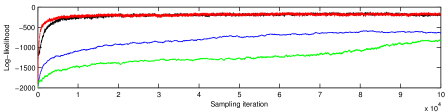
Figure 2: The evolution of the log-likelihood values across all iterations in MNIST dataset for the sampling schemes aGrad-z-gibbs (black line), aGrad-z-joint (red line), Ellipt-gibbs (blue line) and pCNL-gibbs (green line).

6 Discussion

We have shown how to turn simple random walk proposals into gradient-based samplers by the use of auxiliary variables and Taylor approximations. From a methodological side, we provide a framework for producing new algorithms that yields as special cases the standard gradient-based samplers MALA and pCNL. However, the algorithms that we promote in the article and empirically are shown to have a far superior performance are different instances of the generic framework. Our work generates several topics that call for further research. Here we highlight the following four. One is the scaling of the proposed algorithms. A great asset of the new samplers is that they only require the tuning of a single scalar step size, denoted as $\delta$ in the article; we have empirically found that setting it to achieve about 50% to 60% acceptance rate leads to good mixing across a wide range of examples (see Supplement for a plot that empirically illustrates that this range of acceptance rates maximizes ESS), and have shown (in the Supplement) how to adaptively do the tuning without affecting the complexity of the algorithm. Actually, the arguments in Section 3.4 suggest taking $\delta$ as $1/\lambda$, where $\lambda$ is a measure of precision in the likelihood. It would be really interesting to formalise these arguments and even in the context of Gaussian targets obtain an optimal scaling theory in terms of squared jumping distance. The existing results of sherlock are relevant but not directly applicable. A second is the theoretical investigation of the relative efficiency among the auxiliary and the marginal samplers as $n$ or other parameters of the target vary. We have rigorously shown that the asymptotic variance of ergodic averages computed with auxiliary samplers is larger than that for the marginal sampler. We have empirically observed that the efficiency of the aGrad-u is better than that of aGrad-z, hence conforming to the intuition that larger computational cost is associated with better Monte Carlo efficiency. We have also observed empirically that the relative performance among the samplers does not change drastically as $n$ or other parameters vary. It is interesting to obtain solid theoretical results on these comparisons. Thirdly, in this article the dimension of the auxiliary variables, $\mathbf{u}$ or $\mathbf{z}$, matched that of the state vector $\mathbf{x}$. This however does not need to be so. Both the theory on the comparison between marginal and auxiliary samplers, but also the generic methodology as described in Section 2, work also when dimensions of the auxiliary variable and $\mathbf{x}$ are different. We anticipate that even more challenging learning problems than those considered in this paper can benefit from this flexibility. Finally, the well developed Markov chain theory for the convergence of the two-component Gibbs sampler can be used to try and characterise the properties of the idealised Gibbs sampling algorithm that can sample exactly $\pi(\mathbf{x}|\mathbf{u})$. Questions regarding the choice of step size $\delta$, the preconditioner $\mathbf{\Sigma}$ or the augmentation of $\mathbf{u}$ or $\mathbf{z}$, could be answered by obtaining characterisations of the convergence rate of the idealised algorithm.

Appendix/Supplementary material

Reversibility properties of the marginal sampler

We start with proving Lemma 1 in the main paper.

Lemma 2.

1. Suppose that $\mathbf{F}$ is symmetric and commutes with $\mathbf{C}$. Then, the transition density $\mathcal{N}(\mathbf{y}|\mathbf{F}\mathbf{x},(\mathbf{I}-\mathbf{F}^{2})\mathbf{C})$ is reversible with respect to $\mathcal{N}(\mathbf{x}|\bm{0},\mathbf{C})$.

2. Suppose that $\mathbf{C}$ is invertible with $\mathbf{C}=\bm{\Gamma}^{2}$ and $\mathbf{F}$ is symmetric. Then the transition density $\mathcal{N}(\mathbf{y}|\bm{\Gamma}\mathbf{F}\bm{\Gamma}^{-1}\mathbf{x},\bm{\Gamma}(\mathbf{I}-\mathbf{F}^{2})\bm{\Gamma})$ is reversible with respect to $\mathcal{N}(\mathbf{x}|\bm{0},\mathbf{C})$.

Proof.

(a): We need to show that the joint law defined by the prior $\mathcal{N}(\mathrm{d}\mathbf{x}|\bm{0},\mathbf{C})$ and the kernel $\mathcal{N}(\mathrm{d}\mathbf{y}|\mathbf{F}\mathbf{x},(\mathbf{I}-\mathbf{F}^{2})\mathbf{C})$, say $Q(\mathrm{d}\mathbf{x},\mathrm{d}\mathbf{y})$ is symmetric, in the sense that $Q(\mathrm{d}\mathbf{x},\mathrm{d}\mathbf{y})=Q(\mathrm{d}\mathbf{y},\mathrm{d}\mathbf{x})$. With the kernel defined, the joint law defined is jointly Gaussian with mean $\bm{0}$ and covariance

$$\left(\begin{array}[c]{cc}\mathbf{C}&\mathbf{C}\mathbf{F}^{T}\\ \mathbf{F}\mathbf{C}&\mathbf{C}\end{array}\right)=\left(\begin{array}[c]{cc}\mathbf{C}&\mathbf{C}\mathbf{F}\\ \mathbf{C}\mathbf{F}&\mathbf{C}\end{array}\right)$$

where the equality is due to the assumed symmetry and comutability of $\mathbf{F}$. This Gaussian law is symmetric.
(b) Result (a) implies that $\mathcal{N}(\mathrm{d}\mathbf{z};\mathbf{F}\mathbf{u},\mathbf{I}-\mathbf{F}^{2})$ is reversible with respect to $\mathcal{N}(\mathrm{d}\mathbf{u};\bm{0},\mathbf{I})$ when $\mathbf{F}$ is symmetric; let $\tilde{\pi}$ and $\tilde{q}$ denote the target and transition density of these standardized variables. Consider the transformation $\mathbf{x}=\bm{\Gamma}\mathbf{u},\mathbf{y}=\bm{\Gamma}\mathbf{z}$, which is invertible by assumption. Then,

$$\pi(\mathbf{x})q(\mathbf{y}|\mathbf{x}) =|\bm{\Gamma}|^{-2}\pi(\bm{\Gamma}^{-1}\mathbf{u})q(\bm{\Gamma}^{-1}\mathbf{z}|\bm{\Gamma}^{-1}\mathbf{u})=\tilde{\pi}(\mathbf{u})\tilde{q}(\mathbf{z}|\mathbf{u})=\tilde{\pi}(\mathbf{z})\tilde{q}(\mathbf{u}|\mathbf{z})$$

$$=\pi(\mathbf{y})q(\mathbf{x}|\mathbf{y}),$$

where first and last equalities follow from change of variables and the middle one by the established reversibility of the standardized process. ∎

We now show that the marginal sampler proposal is reversible with respect to the prior when $\nabla f=\bm{0}$. Recall that the marginal sampler proposal in that case becomes

$$q(\mathbf{y}|\mathbf{x})=\mathcal{N}\left(\mathbf{y}|({\delta\over 2}\mathbf{I}+\mathbf{C})^{-1}\mathbf{C}\mathbf{x},{\delta\over 2}({\delta\over 2}\mathbf{I}+\mathbf{C})^{-1}(\mathbf{I}+({\delta\over 2}\mathbf{I}+\mathbf{C})^{-1}\mathbf{C})\mathbf{C}\right)\,,$$

by using the alternative expression for $\mathbf{A}$ in Equation (4) of the main article, and after collecting terms. We then work as follows, using Schur’s complement:

$$\mathbf{I}-\left({\delta\over 2}\mathbf{I}+\mathbf{C}\right)^{-1}\mathbf{C} =\mathbf{I}-\mathbf{C}^{1/2}\left({\delta\over 2}\mathbf{I}+\mathbf{C}\right)^{-1}\mathbf{C}^{1/2}$$

$$=\left(\mathbf{I}+\mathbf{C}^{1/2}{2\over\delta}\mathbf{C}^{1/2}\right)^{-1}={\delta\over 2}\left({\delta\over 2}\mathbf{I}+\mathbf{C}\right)^{-1}$$

therefore the variance of the transition density can be written as

$$\left\{\mathbf{I}-\left({\delta\over 2}\mathbf{I}+\mathbf{C}\right)^{-2}\mathbf{C}^{2}\right\}\mathbf{C}=(\mathbf{I}-\mathbf{F}^{2})\mathbf{C},$$

for $\mathbf{F}$ the autoregressive matrix, $\mathbf{F}=\left({\delta\over 2}\mathbf{I}+\mathbf{C}\right)^{-1}\mathbf{C}$.

Second order schemes

Our framework can be easily extended to a second-order Taylor expansion of $f(\mathbf{x})$. For instance the auxiliary sampler based on $\mathbf{u}$ and the corresponding marginal sampler are obtained as follows:

$$q(\mathbf{y}|\mathbf{u},\mathbf{x}) \propto\mathcal{N}\left(\mathbf{y}|\frac{2}{\delta}\mathbf{A}_{\mathbf{x}}\left(\mathbf{u}-\frac{\delta}{2}(\nabla f(\mathbf{x})-\mathbf{H}_{\mathbf{x}}\mathbf{x})\right),\mathbf{A}_{\mathbf{x}}\right)$$

$$q(\mathbf{y}|\mathbf{x})=\mathcal{N}\left(\mathbf{y}|\frac{2}{\delta}\mathbf{A}_{\mathbf{x}}\left(\mathbf{x}-\frac{\delta}{2}(\nabla f(\mathbf{x})-\mathbf{H}_{\mathbf{x}}\mathbf{x})\right),\frac{2}{\delta}\mathbf{A}_{\mathbf{x}}^{2}+\mathbf{A}_{\mathbf{x}}\right)\,,$$

where $\mathbf{H}_{\mathbf{x}}=\nabla\nabla f(\mathbf{x})$, and $\mathbf{A}_{\mathbf{x}}=((2/\delta)\mathbf{I}+\mathbf{C}^{-1}-\mathbf{H}_{\mathbf{x}})^{-1}$. It is straightforward to show that this defines a Gaussian autoregression that is reversible with respect to $\pi(\mathbf{x})$ when $f$ is a quadratic function, since the second-order expansion is now exact. We do not pursue further the construction of second-order schemes since they are computationally prohibitive in high dimensions due to the need for matrix decompositions at each iteration. For such cases, approximations to the Hessian would be needed as those discussed in [28].

Experiments

In all the experiments the ESS has been estimated as proposed in [10] and implemented in the code provided by the authors of [11].

Additional experiments with Gaussian process regression

The three regression datasets along with graphical summaries of MCMC output are plotted in Figure 3. Also in the main article we provide ESS summaries for the experiment with $\sigma^{2}=0.01$. Here we provide for simulations with $\sigma^{2}=1$ and $\sigma^{2}=0.1$, see Table 4 and Table 5 respectively.

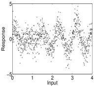
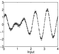
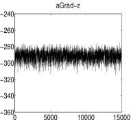
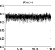
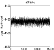
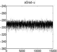
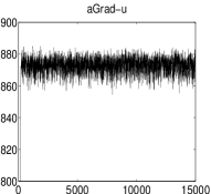
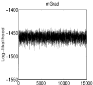
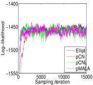
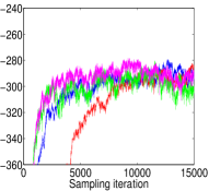
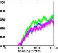
Figure 3: First row shows the three datasets of varying observation noise. The next rows show the evolution of $f(\mathbf{x})$ across iterations for all algorithms. Notice that in the plot at last row and column the log-likelihood values are shown for the first 15000 iterations, while the algorithms were actually run longer to reach convergence (see main text).

Table 4: Comparison of sampling methods in the regression dataset with $\sigma^{2}=1$.

Method Time(s) Step $\delta$ ESS (Min, Med, Max) Min ESS/s (s.d.) aGrad-z 5.5 0.589 (391.7, 517.8, 629.0) 71.05 (6.41) aGrad-u 6.8 0.673 (456.0, 575.2, 696.9) 66.66 (6.28) mGrad 6.0 1.337 (987.4, 1287.5, 1498.4) 167.68 (26.83) pMALA 21.1 0.008 (21.0, 99.1, 274.3) 1.00 (0.28) Ellipt 4.1 (16.7, 66.6, 149.7) 4.03 (1.35) pCN 2.7 0.006 (14.3, 52.3, 130.1) 5.21 (2.40) pCNL 10.5 0.010 (31.9, 125.5, 294.5) 3.03 (0.94)

Table 5: Comparison of sampling methods in the regression dataset with $\sigma^{2}=0.1$.

Method Time(s) Step $\delta$ ESS (Min, Med, Max) Min ESS/s (s.d.) aGrad-z 5.5 0.053 (326.4, 459.9, 575.4) 59.05 (7.92) aGrad-u 6.8 0.060 (360.4, 500.8, 620.1) 52.78 (6.57) mGrad 5.8 0.121 (973.6, 1196.1, 1408.1) 168.11 (10.69) pMALA 21.2 0.001 (12.7, 58.1, 164.4) 0.60 (0.26) Ellipt 4.3 (9.9, 42.4, 138.6) 2.33 (0.81) pCN 2.7 0.001 (8.7, 37.5, 108.5) 3.19 (1.25) pCNL 10.4 0.001 (12.7, 57.4, 208.5) 1.21 (0.59)

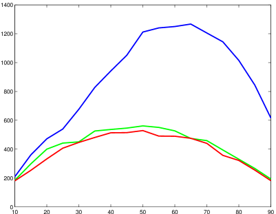
Figure 4: Effective sample size (ESS) shown in the vertical axis versus acceptance rate shown in the horizontal axis for the three proposed algorithms (aGrad-z is shown in red, aGrad-u with green and mGrad with blue). To produce this plot we have repeatedly tuned all algorithms to achieve acceptance rates in a grid of values between 10% and 90%. Then, each time we estimated the ESS based on the first component of the latent vector $\mathbf{x}$. All lines are averages across all three regression datasets and from ten simulation repeats associated with ten different random seeds.

Also, Figure 4 provides an empirical investigation of the optimal acceptance rate for the three proposed algorithms using these regression datasets. This and similar investigations suggest that tuning the step size $\delta$ so that to achieve an acceptance rate around 50% to 60%, as done in all our experiments, is effective.

Additional experiments for log-Gaussian Cox process

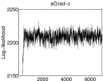
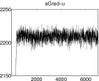
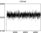
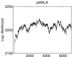
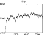
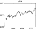
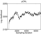
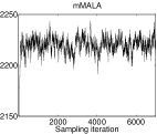
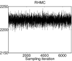
Figure 5: The evolution of the log-likelihood values across all iterations for all sampling schemes in the log-Gaussian Cox process example.

For the original dataset where $\mathbf{x}$ has dimensionality $n=4096$, i.e. the dataset used in the main article, Figure 5 plots the evolution of the log-likelihood $f(\mathbf{x})$ that illustrates convergence and sampling efficiency for all compared algorithms.

Furthermore, in order to investigate how the dimensionality of $\mathbf{x}$ affects performance, we down-sampled the initial dataset by making the mesh grid sparser so that it became of size $32\times 32$. This was done by merging every four neighbouring cells into one (so that the area of a new cell becomes $m=1/1024$) while the observed counts assigned to the initial cells are summed up to form the observed count in the larger cell. This creates a down-sampled dataset where the latent field $\mathbf{x}$ has dimensionality $n=1024$, i.e. four times smaller than the initial dimensionality. Notice that this procedure should keep the likelihood information essentially the same, but we should expect now each likelihood term to become (on average) four times more informative about the value of its latent value $x_{ij}$. We re-run all sampling methods in this down-sampled dataset and Table 6 reports the results. We can observe that the ESS scores remain at the same levels as for the finer grid dataset, while Min ESS/s gets obviously larger due to the smaller running times. A notable feature in Table 6 is that now the step sizes $\delta$ found by aGrad-z, aGrad-u and mGrad become approximately four times smaller than the ones for the finer dataset. This shows that the step sizes are mostly determined by the noise in the likelihood terms, so that in the down-sampled dataset the noise is reduced due to the aggregation of data from the neighbouring cells.

Table 6: Comparison of sampling methods in the log-Gaussian Cox model dataset in the down-sampled version where $n=1024$.

Method Time(s) Step $\delta$ ESS (Min, Med, Max) Min ESS/s (s.d.) aGrad-z 3.5 0.264 (41.0, 202.8, 512.4) 11.76 (1.95) aGrad-u 4.5 0.691 (93.3, 444.2, 1038.7) 21.06 (5.11) mGrad 3.8 1.410 (170.9, 771.1, 1582.7) 46.78 (16.42) pMALA 12.3 0.006 (3.6, 12.6, 53.8) 0.29 (0.02) Ellipt 3.6 (4.7, 17.4, 63.5) 1.32 (0.19) pCN 2.0 0.011 (3.5, 11.7, 50.8) 1.78 (0.32) pCNL 6.0 0.006 (3.6, 12.7, 51.3) 0.59 (0.03) mMALA 17.7 0.070 (22.1, 90.5, 185.5) 1.25 (0.33) RHMC 77.9 0.100 (1747.2, 4601.9, 5000.0) 22.52 (1.94)

Additional experiments with binary regression

Figure 6 shows the evolution of the log-likelihood values for the “Heart” dataset, detailed results for which are shown in the main article. For the rest four datasets such plots look similar. The figure illustrates convergence and sampling efficiency. Tables 7, 10, 8, 9 show the performance of the different sampling schemes in the rest four binary classification datasets.

Table 7: Comparison of sampling methods in Australian Credit dataset. The size of the latent vector $\mathbf{x}$ is $n=690$ and the input dimensionality is $D=14$.

Method Time(s) Step $\delta$ ESS (Min, Med, Max) Min ESS/s (s.d.) aGrad-z 3.0 1.520 (47.0, 153.6, 424.7) 15.50 (4.64) aGrad-u 3.5 2.649 (96.1, 263.2, 647.3) 27.60 (3.89) mGrad 3.0 5.300 (198.2, 504.2, 1191.0) 66.07 (10.03) pMALA 7.0 0.009 (5.1, 21.2, 89.5) 0.73 (0.09) Ellipt 4.3 (6.3, 24.8, 94.7) 1.47 (0.19) pCN 1.7 0.013 (4.2, 17.6, 75.4) 2.56 (0.23) pCNL 2.6 0.009 (5.3, 22.1, 88.8) 2.03 (0.30)

Table 8: Comparison of sampling methods in German Credit dataset. The size of the latent vector x is $n=1000$ and the input dimensionality is $D=24$.

Method Time(s) Step $\delta$ ESS (Min, Med, Max) Min ESS/s (s.d.) aGrad-z 4.4 0.681 (47.1, 161.3, 345.4) 10.74 (1.49) aGrad-u 5.3 1.134 (78.0, 257.0, 518.2) 14.65 (2.66) mGrad 4.5 2.689 (176.0, 528.0, 929.1) 38.73 (6.63) pMALA 15.4 0.016 (6.4, 26.6, 91.6) 0.42 (0.06) Ellipt 5.4 (4.6, 19.8, 66.7) 0.85 (0.07) pCN 2.6 0.013 (3.8, 14.6, 60.5) 1.48 (0.14) pCNL 7.7 0.016 (6.2, 26.4, 92.1) 0.81 (0.11)

Table 9: Comparison of sampling methods in Pima Indian dataset. The size of the latent vector $\mathbf{x}$ is $n=532$ and the input dimensionality is $D=7$.

Method Time(s) Step $\delta$ ESS (Min, Med, Max) Min ESS/s (s.d.) aGrad-z 2.5 1.667 (96.6, 299.1, 735.5) 39.25 (9.70) aGrad-u 2.9 2.943 (176.0, 529.8, 1072.6) 60.66 (6.49) mGrad 2.4 6.134 (322.2, 947.8, 1594.5) 133.75 (13.25) pMALA 3.6 0.053 (28.4, 93.0, 233.0) 7.93 (2.16) Ellipt 3.2 (19.2, 66.6, 175.4) 6.06 (1.28) pCN 1.4 0.055 (12.2, 43.1, 128.7) 8.73 (1.16) pCNL 2.1 0.056 (27.8, 93.0, 235.9) 13.35 (3.46)

Table 10: Comparison of sampling methods in Ripley dataset. The size of the latent vector $\mathbf{x}$ is $n=250$ and the input dimensionality is $D=2$.

Method Time(s) Step $\delta$ ESS (Min, Med, Max) Min ESS/s (s.d.) aGrad-z 1.3 3.589 (21.5, 125.5, 630.0) 16.58 (7.09) aGrad-u 1.4 4.526 (28.8, 163.5, 805.3) 19.95 (8.43) mGrad 1.2 9.014 (47.0, 289.4, 1730.3) 38.04 (11.87) pMALA 1.5 0.017 (13.8, 58.2, 240.4) 8.94 (0.87) Ellipt 1.9 (11.2, 51.2, 206.9) 5.76 (1.63) pCN 0.7 0.019 (7.3, 30.9, 140.6) 10.70 (3.51) pCNL 1.1 0.017 (14.3, 56.1, 222.1) 13.09 (3.25)

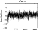
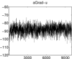
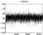
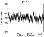
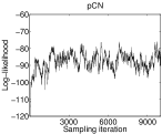
Figure 6: The evolution of the log-likelihood values across all iterations for the sampling schemes aGrad-z, aGrad-u, mGrad-z, pMALA, pCN and pCNL in the Heart dataset. The corresponding plot for Ellipt looks very similar to pCN and it is omitted.

Additional experiments for hyperparameter learning

In the first experiment we consider binary Gaussian process classification and we apply the alternative schemes to Pima Indian dataset. We run the algorithms for $4\times 10^{4}$ burn-in iteration and then we collect $5\times 10^{3}$ samples. Figure 7 shows the log-likelihoods across all $4.5\times 10^{4}$ sampling iterations. We can observe that aGrad-z-joint is the best mixing with aGrad-z-gibbs coming second. The corresponding plots for Ellipt-gibbs and pCNL-gibbs exhibit less variation, and stabilize in slightly smaller log-likelihood values, with pCNL being the most problematic. Figure 8 shows boxplots for the inferred hyperparameters for the different methods. We observe that while aGrad-z-gibbs and aGrad-z-joint largely agree about the inferred values, Ellipt-gibbs and pCNL-gibbs have very narrow boxplots. Also pCNL-gibbs clearly has stuck to a posterior mode which is rather very different from the remaining algorithms. Finally, Table 11 shows performance scores for sampling the two hyperparameters which show the clear superiority of aGrad-z-joint. Notice that the learned step size $\kappa$ is much larger for aGrad-z-joint than for the remaining schemes. Notice, however, that the ESS scores for Ellipt-gibbs and pCNL-gibbs should not be trusted since Figure 7 and Figure 8 suggest that these methods do not mix well.

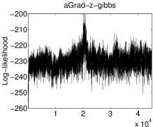
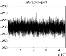
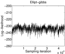
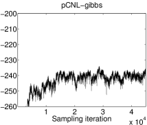
Figure 7: The evolution of the log-likelihood values across all iterations in Pima Indian.

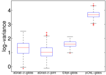
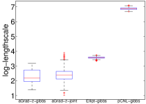
Figure 8: The inferred hyperparameters values in Pima Indian dataset.

Table 11: Performance scores of the sampling methods in Pima dataset for the kernel hyperparameters.

Method Time(s) Step $\kappa$ ESS ($\sigma_{x}^{2}$, $\ell^{2}$) Min ESS/s aGrad-z-gibbs 599.4 0.005 (5.1, 11.0) 0.01 aGrad-z-joint 692.6 0.179 (173.4, 232.5) 0.25 Ellipt-gibbs 426.8 0.006 (3.2, 5.7) 0.01 pCNL-gibbs 350.7 0.020 (4.4, 15.3) 0.01

Efficient implementation of the algorithms

Pilot tuning of step size

All algorithms discussed in the main article require the choice of a single step size parameter $\delta$ in order to achieve an acceptance rate that leads to good mixing. In our experiments all algorithms that use gradient information are tuned to achieve an acceptance rate around 50%; asymptotic theory, e.g. in [21], supports this tuning for pMALA, this is the rate that pCNL is tuned to in experiments in [4] and rate that our experiments suggests to be advantageous for the new auxiliary and marginal samplers. On the other hand, pCN is tuned to achieve a rate around 30% following the recommendation in [4]. A simple observation is that no matrix factorisations are needed during the tuning as we adapt $\delta$, since all matrices involved in the algorithms, either when $\mathbf{\Sigma}=\mathbf{I}$ or $\mathbf{\Sigma}=\mathbf{C}$, share the same eigenspace with $\mathbf{C}$ regardless of the value of $\delta$, hence an offline spectral decomposition of the latter (e.g. using a QR-algorithm) can be easily updated at $\mathcal{O}(n)$ cost to produce all matrices necessary to carry out the algorithms. Additional details regarding the implementation of the algorithms is given in the next section.

Efficient generation of proposal, computation of acceptance ratio and pseudocode for the proposed algorithms

Here, we discuss how we can efficiently implement all algorithms based on a eigenvalue decomposition of the prior covariance matrix $\mathbf{C}$. We provide full details for the proposed marginal sampler, while for all remaining schemes the implementation follows similar steps.

The marginal scheme has proposal

$$q(\mathbf{y}|\mathbf{x})=\mathcal{N}\left(\mathbf{y}|{2\over\delta}\mathbf{A}\left(\mathbf{x}+{\delta\over 2}\nabla f(\mathbf{x})\right),{2\over\delta}\mathbf{A}^{2}+\mathbf{A}\right)\,$$ (12)

where $\mathbf{A}^{-1}=\mathbf{C}^{-1}+{2\over\delta}\mathbf{I}$ and the corresponding Metropolis-Hastings ratio is

$$\exp\{f(\mathbf{y})-f(\mathbf{x})+h(\mathbf{x},\mathbf{y})-h(\mathbf{y},\mathbf{x})\},$$ (13)

$$h(\mathbf{x},\mathbf{y})=\left(\mathbf{x}-\frac{2}{\delta}\mathbf{A}(\mathbf{y}+{\delta\over 4}\nabla f(\mathbf{y}))\right)^{T}\left({2\over\delta}\mathbf{A}+\mathbf{I}\right)^{-1}\nabla f(\mathbf{y})\,$$

To provide an efficient implementation we will be based on a precomputed decomposition of $\mathbf{C}=\mathbf{U}\bm{\Lambda}\mathbf{U}^{T}$. Based on this $\mathbf{A}$ can be written as

$$\mathbf{A}=\mathbf{U}\bm{\Lambda}_{1}\mathbf{U}^{T}$$

where each eigenvalue in the diagonal matrix $\bm{\Lambda}_{1}$ has the form $\frac{\gamma\delta}{\delta+2\gamma}$ where $\gamma$ is an eigenvalue of $\mathbf{C}$. Similarly

$${2\over\delta}\mathbf{A}^{2}+\mathbf{A}=\mathbf{U}\bm{\Lambda}_{2}\mathbf{U}^{T}$$

where each eigenvalue of $\bm{\Lambda}_{2}$ has the form $\frac{\gamma\delta}{\delta+2\gamma}\times\frac{\delta+4\gamma}{\delta+2\gamma}$. Also it would be useful to know the decomposition of $\left({2\over\delta}\mathbf{A}+\mathbf{I}\right)^{-1}$ which is

$$\left({2\over\delta}\mathbf{A}+\mathbf{I}\right)^{-1}=\mathbf{U}\bm{\Lambda}_{3}\mathbf{U}^{T}$$

where each eigenvalue of $\bm{\Lambda}_{3}$ has the form $\frac{\delta+2\gamma}{\delta+4\gamma}$. A sample from $q(\mathbf{y}|\mathbf{x})$ can be implemented as follows

$$\mathbf{y}=\mathbf{U}\left[\bm{\Lambda}_{1}\left({2\over\delta}\mathbf{U}^{T}\mathbf{x}+\mathbf{U}^{T}\nabla f(\mathbf{x})\right)+\bm{\Lambda}_{2}^{\frac{1}{2}}\bm{\eta}\right],\ \ \text{where}\ \ \bm{\eta}\sim\mathcal{N}(\bm{0},\mathbf{I}).$$

To compute this term we consider that the vectors $\mathbf{U}^{T}\mathbf{x}$, $\mathbf{U}^{T}\nabla f(\mathbf{x})$ and the whole $\bm{\Lambda}_{1}\left({2\over\delta}\mathbf{U}^{T}\mathbf{x}+\mathbf{U}^{T}\nabla f(\mathbf{x})\right)$ have already been pre-computed from a previous MCMC iteration. Therefore, the above sampling operation involves the computation of $\bm{\Lambda}_{1}^{\frac{1}{2}}\bm{\eta}$, which costs $\mathcal{O}(n)$ since $\bm{\Lambda}_{1}^{\frac{1}{2}}$ is diagonal, an addition of two vectors and a single matrix-vector multiplication involving the most-left $\mathbf{U}$ and the remaining term (which is just an already computed vector). Thus, overall the proposal of $\mathbf{y}$ can be implemented with a single matrix-vector multiplication, which costs $\mathcal{O}(n^{2})$.

The computation of the Metropolis-Hastings ratio can be carried out as follows. To compute $h(\mathbf{x},\mathbf{y})$ we are based on the expression

$$h(\mathbf{x},\mathbf{y}) =\left(\mathbf{x}-\mathbf{U}\bm{\Lambda}_{1}(\frac{2}{\delta}\mathbf{U}^{T}\mathbf{y}+{1\over 2}\mathbf{U}^{T}\nabla f(\mathbf{y}))\right)^{T}\mathbf{U}\bm{\Lambda}_{3}\mathbf{U}^{T}\nabla f(\mathbf{y})$$

$$=\left[\mathbf{U}^{T}\mathbf{x}-\left(\bm{\Lambda}_{1}(\frac{2}{\delta}\mathbf{U}^{T}\mathbf{y}+{1\over 2}\mathbf{U}^{T}\nabla f(\mathbf{y}))\right)\right]^{T}\bm{\Lambda}_{3}\mathbf{U}^{T}\nabla f(\mathbf{y})$$

Then, we apply two matrix-vector multiplications, each having cost $\mathcal{O}(n^{2})$, in order to compute the vectors $\mathbf{U}^{T}\mathbf{y}$ and $\mathbf{U}^{T}\nabla f(\mathbf{y})$. With these two vectors pre-computed and stored all remaining operations cost $\mathcal{O}(n)$. For example, the computation of $\bm{\Lambda}_{3}\mathbf{U}^{T}\nabla f(\mathbf{y})$ is $\mathcal{O}(n)$ since $\bm{\Lambda}_{3}$ is diagonal. Also the computation of the symmetric term $h(\mathbf{y},\mathbf{x})$ required in the ratio is just $\mathcal{O}(n)$ since the required vectors $\mathbf{U}^{T}\mathbf{x}$ and $\mathbf{U}^{T}\nabla f(\mathbf{x})$ are known form the previous iteration. Notice that if $\mathbf{y}$ is accepted, then the two vectors $\mathbf{U}^{T}\mathbf{y}$ and $\mathbf{U}^{T}\nabla f(\mathbf{y})$ will become the already pre-computed vectors required in the next iteration. Also when $\mathbf{y}$ is accepted we also compute $\bm{\Lambda}_{1}(\frac{2}{\delta}\mathbf{U}^{T}\mathbf{y}+\mathbf{U}^{T}\nabla f(\mathbf{y}))$ needed for the upcoming proposal step in the next iteration. So overall, the marginal scheme requires three matrix-vector multiplications per iteration.

Working similarly as above, the auxiliary scheme based on $\mathbf{u}$ can be implemented with three matrix-vector multiplications per iteration, the auxiliary scheme based on $\mathbf{z}$ as well as pCNL require two such operations, while the pCN scheme requires just a single matrix-vector multiplication per iteration. Full pseudocode for all three proposed algorithms aGrad-z, aGrad-u and mGrad is given by Algorithm 1, Algorithm 2 and Algorithm 3 respectively. The appearance of $*$s indicate the number and the precise lines inside the code we need to perform a matrix-vector multiplication.

Algorithm 1 aGrad-z

  Input: $\mathbf{U}$ and $\bm{\Gamma}$ such that $\mathbf{U}\bm{\Gamma}\mathbf{U}^{T}=\mathbf{C}$, $f(\mathbf{x})$, $\nabla f(\mathbf{x})$, number of burn-in and collection iterations BURN and T.

  Initialize: $\mathbf{x}={\bf 0}$, $f\mathbf{x}=f(\mathbf{x})$, $\text{grad}f\mathbf{x}=\nabla f(\mathbf{x})$, the diagonal $\bm{\Lambda}_{1}$ such that $[\bm{\Lambda}_{1}]_{ii}=\frac{\gamma_{i}\delta}{\delta+2\gamma_{i}}$.

  for $i=1$ to $\text{BURN}+\text{T}$ do

     Draw $\mathbf{z}=\mathbf{x}+(\delta/2)\text{grad}f\mathbf{x}+\sqrt{\delta/2}\bm{\eta},\ \ \ \bm{\eta}\sim\mathcal{N}({\bf 0},\mathbf{I})$.

     Propose $\mathbf{y}=\mathbf{U}\left(\bm{\Lambda}_{1}^{\frac{1}{2}}\left(\bm{\Lambda}_{1}^{\frac{1}{2}}(\mathbf{U}^{T}(\frac{2}{\delta}\mathbf{z}))+\bm{\eta}\right)\right),\ \ \ \bm{\eta}\sim\mathcal{N}({\bf 0},\mathbf{I})$.          **

     M-H step: $f\mathbf{y}=f(\mathbf{y})$, $\text{grad}f\mathbf{y}=\nabla f(\mathbf{y})$,         $g\mathbf{z}\mathbf{y}=(\mathbf{z}-\mathbf{y}-\frac{\delta}{4}\text{grad}f\mathbf{y})^{T}\text{grad}f\mathbf{y}$,        $g\mathbf{z}\mathbf{x}=(\mathbf{z}-\mathbf{x}-\frac{\delta}{4}\text{grad}f\mathbf{x})^{T}\text{grad}f\mathbf{x}$.        if $rand<min(1,\exp(f\mathbf{y}-f\mathbf{x}+g\mathbf{z}\mathbf{y}-g\mathbf{z}\mathbf{x}))$ then           $\mathbf{x}=\mathbf{y}$, $f\mathbf{x}=f\mathbf{y}$, $\text{grad}f\mathbf{x}=\text{grad}f\mathbf{y}$.        end if

     Adapt $\delta$ or collect sample:        if $i\leq$ BURN            adapt $\delta$ to achieve acceptance rate in $50\%$ to $60\%$.           update $\bm{\Lambda}_{1}$: $[\bm{\Lambda}_{1}]_{ii}=\frac{\gamma_{i}\delta}{\delta+2\gamma_{i}}$.        else            collect sample $\mathbf{x}$.        end if

  end for

Algorithm 2 aGrad-u

  Input: $\mathbf{U}$ and $\bm{\Gamma}$ such that $\mathbf{U}\bm{\Gamma}\mathbf{U}^{T}=\mathbf{C}$, $f(\mathbf{x})$, $\nabla f(\mathbf{x})$, number of burn-in and collection iterations BURN and T.

  Initialize: $\mathbf{x}={\bf 0}$, $f\mathbf{x}=f(\mathbf{x})$, $\text{grad}f\mathbf{x}=\nabla f(\mathbf{x})$, $\text{Ugrad}f\mathbf{x}=\mathbf{U}^{T}\text{grad}f\mathbf{x}$, the diagonal $\bm{\Lambda}_{1}$ such that $[\bm{\Lambda}_{1}]_{ii}=\frac{\gamma_{i}\delta}{\delta+2\gamma_{i}}$.

  for $i=1$ to $\text{BURN}+\text{T}$ do

     Draw $\mathbf{u}=\mathbf{x}+\sqrt{\delta/2}\bm{\eta},\ \ \ \bm{\eta}\sim\mathcal{N}({\bf 0},\mathbf{I})$.

     $\text{Udelta}\mathbf{u}=\mathbf{U}^{T}(\frac{2}{\delta}\mathbf{u})$.                                                              *

     Propose $\mathbf{y}=\mathbf{U}\left(\bm{\Lambda}_{1}\left(\text{Udelta}\mathbf{u}+\text{Ugrad}f\mathbf{x}\right)+\bm{\Lambda}_{1}^{\frac{1}{2}}\bm{\eta}\right),\ \bm{\eta}\sim\mathcal{N}({\bf 0},\mathbf{I})$.  *

     M-H step: $f\mathbf{y}=f(\mathbf{y})$, $\text{grad}f\mathbf{y}=\nabla f(\mathbf{y})$, $\text{Ugrad}f\mathbf{y}=\mathbf{U}^{T}\text{grad}f\mathbf{y}$,    *         $j\mathbf{x}\mathbf{y}\mathbf{u}=\mathbf{x}^{T}\text{grad}f\mathbf{y}-\left(\bm{\Lambda}_{1}(\text{Udelta}\mathbf{u}+\frac{1}{2}\text{Ugrad}f\mathbf{y})\right)^{T}\text{Ugrad}f\mathbf{y}$,         $j\mathbf{y}\mathbf{x}\mathbf{u}=\mathbf{y}^{T}\text{grad}f\mathbf{x}-\left(\bm{\Lambda}_{1}(\text{Udelta}\mathbf{u}+\frac{1}{2}\text{Ugrad}f\mathbf{x})\right)^{T}\text{Ugrad}f\mathbf{x}$.        if $rand<min(1,\exp(f\mathbf{y}-f\mathbf{x}+j\mathbf{x}\mathbf{y}\mathbf{u}-j\mathbf{y}\mathbf{x}\mathbf{u}))$ then           $\mathbf{x}=\mathbf{y}$, $f\mathbf{x}=f\mathbf{y}$, $\text{grad}f\mathbf{x}=\text{grad}\mathbf{y}$, $\text{Ugrad}f\mathbf{x}=\text{Ugrad}f\mathbf{y}$.        end if

     Adapt $\delta$ or collect sample:        if $i\leq$ BURN            adapt $\delta$ to achieve acceptance rate in $50\%$ to $60\%$.           update $\bm{\Lambda}_{1}$: $[\bm{\Lambda}_{1}]_{ii}=\frac{\gamma_{i}\delta}{\delta+2\gamma_{i}}$.        else            collect sample $\mathbf{x}$.        end if

  end for

Algorithm 3 mGrad

  Input: $\mathbf{U}$ and $\bm{\Gamma}$ such that $\mathbf{U}\bm{\Gamma}\mathbf{U}^{T}=\mathbf{C}$, $f(\mathbf{x})$, $\nabla f(\mathbf{x})$, number of burn-in and collection iterations BURN and T.

  Initialize: $\mathbf{x}={\bf 0}$, $f\mathbf{x}=f(\mathbf{x})$, $\text{grad}f\mathbf{x}=\nabla f(\mathbf{x})$, $\text{U}\mathbf{x}=\mathbf{U}^{T}\mathbf{x}$, $\text{Ugrad}f\mathbf{x}=\mathbf{U}^{T}\text{grad}f\mathbf{x}$, $\bm{\Lambda}_{1}$ such that $[\bm{\Lambda}_{1}]_{ii}=\frac{\gamma_{i}\delta}{\delta+2\gamma_{i}}$, $\bm{\Lambda}_{2}$ such that $[\bm{\Lambda}_{2}]_{ii}=\frac{\gamma_{i}\delta}{\delta+2\gamma_{i}}\times\frac{\delta+4\gamma_{i}}{\delta+2\gamma_{i}}$, $\bm{\Lambda}_{3}$ such that $[\bm{\Lambda}_{3}]_{ii}=\frac{\delta+2\gamma_{i}}{\delta+4\gamma_{i}}$, $\text{tmpSample}\mathbf{x}=\bm{\Lambda}_{1}\left(\frac{2}{\delta}\text{U}\mathbf{x}+\text{Ugrad}f\mathbf{x}\right)$, $\text{tmpMH}\mathbf{x}=\bm{\Lambda}_{1}\left(\frac{2}{\delta}\text{U}\mathbf{x}+\frac{1}{2}\text{Ugrad}f\mathbf{x}\right)$.

  for $i=1$ to $\text{BURN}+\text{T}$ do

     Propose $\mathbf{y}=\mathbf{U}\left(\text{tmpSample}\mathbf{x}+\bm{\Lambda}_{2}^{\frac{1}{2}}\bm{\eta}\right),\ \ \ \bm{\eta}\sim\mathcal{N}({\bf 0},\mathbf{I})$.                  *

     M-H step: $f\mathbf{y}=f(\mathbf{y})$, $\text{grad}f\mathbf{y}=\nabla f(\mathbf{y})$,       $\text{U}\mathbf{y}=\mathbf{U}^{T}\mathbf{y}$, $\text{Ugrad}f\mathbf{y}=\mathbf{U}^{T}\text{grad}f\mathbf{y}$,                                  **       $\text{tmpSample}\mathbf{y}=\bm{\Lambda}_{1}\left(\frac{2}{\delta}\text{U}\mathbf{y}+\text{Ugrad}f\mathbf{y}\right)$,       $\text{tmpMH}\mathbf{y}=\bm{\Lambda}_{1}\left(\frac{2}{\delta}\text{U}\mathbf{y}+\frac{1}{2}\text{Ugrad}f\mathbf{y}\right)$,       $h\mathbf{x}\mathbf{y}=(\text{U}\mathbf{x}-\text{tmpMH}\mathbf{y})^{T}(\bm{\Lambda}_{3}\text{Ugrad}f\mathbf{y}$),        $h\mathbf{y}\mathbf{x}=(\text{U}\mathbf{y}-\text{tmpMH}\mathbf{x})^{T}(\bm{\Lambda}_{3}\text{Ugrad}f\mathbf{x}$),        if $rand<min(1,\exp(f\mathbf{y}-f\mathbf{x}+h\mathbf{x}\mathbf{y}-h\mathbf{y}\mathbf{x}))$ then           $\mathbf{x}=\mathbf{y}$, $f\mathbf{x}=f\mathbf{y}$, $\text{grad}f\mathbf{x}=\text{grad}f\mathbf{y}$,           $\text{U}\mathbf{x}=\text{U}\mathbf{y}$, $\text{Ugrad}f\mathbf{x}=\text{Ugrad}f\mathbf{y}$,            $\text{tmpSample}\mathbf{x}=\text{tmpSample}\mathbf{y}$, $\text{tmpMH}\mathbf{x}=\text{tmpMH}\mathbf{y}$.        end if

     Adapt $\delta$ or collect sample:        if $i\leq$ BURN            adapt $\delta$ to achieve acceptance rate in $50\%$ to $60\%$.           update $\bm{\Lambda}_{1}$: $[\bm{\Lambda}_{1}]_{ii}=\frac{\gamma_{i}\delta}{\delta+2\gamma_{i}}$.            update $\bm{\Lambda}_{2}$: $[\bm{\Lambda}_{2}]_{ii}=\frac{\gamma_{i}\delta}{\delta+2\gamma_{i}}\times\frac{\delta+4\gamma_{i}}{\delta+2\gamma_{i}}$,            update $\bm{\Lambda}_{3}$: $[\bm{\Lambda}_{3}]_{ii}=\frac{\delta+2\gamma_{i}}{\delta+4\gamma_{i}}$,            update $\text{tmpSample}\mathbf{x}=\bm{\Lambda}_{1}\left(\frac{2}{\delta}\text{U}\mathbf{x}+\text{Ugrad}f\mathbf{x}\right)$,            update $\text{tmpMH}\mathbf{x}=\bm{\Lambda}_{1}\left(\frac{2}{\delta}\text{U}\mathbf{x}+\frac{1}{2}\text{Ugrad}f\mathbf{x}\right)$.        else           collect sample $\mathbf{x}$.        end if

  end for

References

- [1] Christophe Andrieu and Matti Vihola. Convergence properties of pseudo-marginal Markov chain Monte Carlo algorithms. Ann. Appl. Probab., 25(2):1030–1077, 2015.
- [2] M.R. Bass and S.K. Sahu. Effcient parameterisations of Gaussian process based models for Bayesian computation using MCMC. http://www.southampton.ac.uk/sks/research/papers/final_cpvsncp.pdf, 2016.
- [3] Alexandros Beskos, Gareth Roberts, Andrew Stuart, and Jochen Voss. MCMC methods for diffusion bridges. Stoch. Dyn., 8(3):319–350, 2008.
- [4] S. L. Cotter, G. O. Roberts, A. M. Stuart, and D. White. MCMC methods for functions: modifying old algorithms to make them faster. Statistical Science, 28(3):424–446, 2013.
- [5] Tiangang Cui, Kody J. H. Law, and Youssef M. Marzouk. Dimension-independent likelihood-informed MCMC. J. Comput. Phys., 304:109–137, 2016.
- [6] Arnak Dalalyan. Theoretical guarantees for approximate sampling from a smooth and log-concave density. Journal of the Royal Statistical Society. Series B. Statistical Methodology, 3:651–676, 2017.
- [7] Alexander Davies. Effective implementation of Gaussian process regression for machine learning. PhD thesis, Cambridge, 2015.
- [8] Alain Durmus and Eric Moulines. Non-asymptotic convergence analysis for the unadjusted Langevin algorithm. http://arxiv.org/abs/1507.05021, 2016.
- [9] Maurizio Filippone, Mingjun Zhong, and Mark Girolami. A comparative evaluation of stochastic-based inference methods for Gaussian process models. Machine Learning, 93(1):93–114, 2013.
- [10] Charles J Geyer. Practical markov chain monte carlo. Statistical Science, pages 473–483, 1992.
- [11] Mark Girolami and Ben Calderhead. Riemann manifold Langevin and Hamiltonian Monte Carlo methods. Journal of the Royal Statistical Society: Series B (Statistical Methodology), 73(2):123–214, 2011.
- [12] James Hensman, Alexander Matthews, Maurizio Filippone, and Zoubin Ghahramani. MCMC for variationally sparse Gaussian processes. NIPS, 2015.
- [13] L. Knorr-Held and H. Rue. On Block Updating in Markov Random Field Models for Disease Mapping. Scandinavian Journal of Statistics, 29(4):597–614, December 2002.
- [14] K. J. H. Law. Proposals which speed up function-space MCMC. J. Comput. Appl. Math., 262:127–138, 2014.
- [15] Fabrizio Leisen and Antonietta Mira. An extension of Peskun and Tierney orderings to continuous time Markov chains. Statist. Sinica, 18(4):1641–1651, 2008.
- [16] Iain Murray and Ryan Prescott Adams. Slice sampling covariance hyperparameters of latent Gaussian models. In J. Lafferty, C. K. I. Williams, R. Zemel, J. Shawe-Taylor, and A. Culotta, editors, Advances in Neural Information Processing Systems 23, pages 1723–1731. 2010.
- [17] Iain Murray, Ryan Prescott Adams, and David J.C. MacKay. Elliptical slice sampling. JMLR: W&CP, 9:541–548, 2010.
- [18] Radford M. Neal. Regression and classification using Gaussian process priors. In Bayesian statistics, 6 (Alcoceber, 1998), pages 475–501. Oxford Univ. Press, New York, 1999.
- [19] Omiros Papaspiliopoulos, Gareth O. Roberts, and Martin Sköld. Non-centered parameterizations for hierarchical models and data augmentation. In Bayesian statistics, 7 (Tenerife, 2002), pages 307–326. Oxford Univ. Press, New York, 2003. With a discussion by Alan E. Gelfand, Ole F. Christensen and Darren J. Wilkinson, and a reply by the authors.
- [20] P. H. Peskun. Optimum Monte-Carlo sampling using Markov chains. Biometrika, 60:607–612, 1973.
- [21] Gareth O. Roberts and Jeffrey S. Rosenthal. Optimal scaling for various Metropolis-Hastings algorithms. Statist. Sci., 16(4):351–367, 2001.
- [22] Gareth O. Roberts and Richard L. Tweedie. Exponential convergence of Langevin distributions and their discrete approximations. Bernoulli, 2(4):341–363, 1996.
- [23] Chris Sherlock and Gareth Roberts. Optimal scaling of the random walk Metropolis on elliptically symmetric unimodal targets. Bernoulli, 15(3):774–798, 2009.
- [24] Geir Storvik. On the flexibility of Metropolis-Hastings acceptance probabilities in auxiliary variable proposal generation. Scand. J. Stat., 38(2):342–358, 2011.
- [25] Yee Whye Teh and Max Welling. Bayesian learning via stochastic gradient Langevin dynamics. In nternational Conference on Machine Learning, pages 1723–1731. 2011.
- [26] Luke Tierney. A note on Metropolis-Hastings kernels for general state spaces. Ann. Appl. Probab., 8(1):1–9, 1998.
- [27] Michalis K. Titsias. Contribution to the discussion of the paper by Girolami and Calderhead. Journal of the Royal Statistical Society: Series B (Statistical Methodology), 73(2):197–199, 2011.
- [28] Yichuan Zhang and Charles A. Sutton. Quasi-newton methods for markov chain monte carlo. In Advances in Neural Information Processing Systems 24: 25th Annual Conference on Neural Information Processing Systems 2011. Proceedings of a meeting held 12-14 December 2011, Granada, Spain., pages 2393–2401, 2011.