Theory of surface Andreev bound states and tunneling spectroscopy in three-dimensional chiral superconductors

Abstract

We study the surface Andreev bound states (SABSs) and quasiparticle tunneling spectroscopy of three-dimensional (3D) chiral superconductors by changing their surface (interface) misorientation angles. We obtain an analytical formula for the SABS energy dispersion of a general pair potential, for which an original $4\times 4$ BdG Hamiltonian can be reduced to two $2\times 2$ blocks. The resulting SABS for 3D chiral superconductors with a pair potential given by $k_{z}(k_{x}+ik_{y})^{\nu}$ ($\nu=1,2$) has a complicated energy dispersion owing to the coexistence of both point and line nodes. We focus on the tunneling spectroscopy of this pairing in the presence of an applied magnetic field, which induces a Doppler shift in the quasiparticle spectra. In contrast to the previously known Doppler effect in unconventional superconductors, a zero bias conductance dip can change into a zero bias conductance peak owing to an external magnetic field. We also study SABSs and tunneling spectroscopy for possible pairing symmetries of UPt₃. For this purpose, we extend a standard formula for the tunneling conductance of unconventional superconductor junctions to treat spin-triplet non-unitary pairings. Magneto tunneling spectroscopy, $i.e$., tunneling spectroscopy in the presence of a magnetic field, can serve as a guide to determine the pairing symmetry of this material.

I Introduction

The surface Andreev bound state (SABS) is one of the key concepts regarding unconventional superconductors Kashiwaya and Tanaka (2000); Löfwander et al. (2001); Golubov et al. (2004). To date, various types of SABSs have been revealed in two-dimensional (2D) unconventional superconductors Tanaka et al. (2012); Qi and Zhang (2011). It is known that a flat band SABS exists in a spin-singlet $d$-wave superconductor Hu (1994) that is protected by a topological invariant defined in the bulk Hamiltonian Ryu and Hatsugai (2002); Sato et al. (2011a); Tanaka et al. (2012); Sato and Fujimoto (2016). The ubiquitous presence of this zero energy SABS manifests itself as a zero bias conductance peak (ZBCP) in the tunneling spectroscopy of high-$T_{c}$ cuprates Tanaka and Kashiwaya (1995); Kashiwaya et al. (1995a, 1998); Covington et al. (1997); Alff et al. (1997); Wei et al. (1998); Biswas et al. (2002). There has been interest in the spin-triplet $p$-wave superconductorBuchholtz and Zwicknagl (1981); Hara and Nagai (1986) with a flat band SABS and sharp ZBCP, similar to the $d$-wave case Yamashiro et al. (1998); Tanaka et al. (2002a); Kwon et al. (2004). Apart from flat bands, it is known that chiral $p$-wave superconductors host an SABS with a linear dispersion as a function of momentum parallel to the edge, resulting in a much broader ZBCP Yamashiro et al. (1997); Honerkamp and Sigristt (1998); Kashiwaya et al. (2011); Kwon et al. (2004); Wu and Samokhin (2010).

Magneto tunneling spectroscopy, $i$.$e$., tunneling spectroscopy in the presence of an applied magnetic field, is a powerful tool to make distinctions among pairing symmetries. Under an applied magnetic field, the shift of quasiparticle energy spectra, which is proportional to the transverse momentum, is generally known as the Doppler effectFogelström et al. (1997); Covington et al. (1997). It has been shown that the splitting of the ZBCP occurs in $d$-wave superconductor junctions owing to thisFogelström et al. (1997); Covington et al. (1997). In contrast, for spin-triplet $p$-wave cases, the ZBCP does not split into twoTanaka et al. (2002a) since the perpendicular injection of quasiparticles dominantly contributes to the tunneling conductance. For perpendicular injection, the component of the Fermi velocity parallel to the interface is zero and there is no energy shift of the quasiparticles. Therefore, we can distinguish between $d$- and $p$-wave pairing with magneto tunneling spectroscopyTanuma et al. (2002a). For chiral $p$-wave superconductors, the magnitude of the ZBCP is enhanced or suppressed depending on the direction of the applied magnetic fieldTanaka et al. (2002a). Chiral and helical superconductors also exhibit different features of magneto tunneling spectroscopy, whereas both of these superconductors have similarly broad ZBCP without magnetic fieldTanaka et al. (2009). In any case, a ZBCP generated from a zero bias conductance dip by applying magnetic field has not been found.

For three-dimensional (3D) unconventional superconductors, the energy dispersion of SABS becomes more complicated Buchholtz and Zwicknagl (1981); Qi et al. (2009); Chung and Zhang (2009); Murakawa et al. (2009); Asano et al. (2003); Fu and Berg (2010); Sasaki et al. (2011); Hao and Lee (2011); Hsieh and Fu (2012); Yamakage et al. (2012); Hashimoto et al. (2015); Lu et al. (2015); Hashimoto et al. (2016). Recently, the SABSs of 3D chiral superconductors have been studied Kobayashi et al. (2015), where a pair potential is given by $\Delta_{0}k_{z}(k_{x}+ik_{y})^{\nu}/k_{\mathrm{F}}^{\nu+1}$ with a nonzero integer $\nu$. These pairing symmetries are relevant to typical heavy fermion superconductors with $\nu=1$ and $\nu=2$, corresponding to the candidate pairing symmetries of URu₂Si₂ Schemm et al. (2015a); Kasahara et al. (2007); Shibauchi et al. (2014); Schemm et al. (2015b) and UPt₃ Sauls (1994); Joynt and Taillefer (2002); Schemm et al. (2014); Goswami and Nevidomskyy (2015); Tsutsumi et al. (2012, 2013) respectively. The simultaneous presence of line and point nodes gives rise to exotic SABS. It has been shown that the flat band SABS is found to be fragile against the surface misorientation angle $\alpha$, as shown in Fig. 1. Although the topological natures of the flat band SABS have been clarified Kobayashi et al. (2015), the overall features of the energy dispersion of the SABS have not been systematically analyzed. Thus, it is a challenging issue to identify 3D pairing states theoretically in terms of magneto tunneling spectroscopy.

In this work, we study the SABS and quasiparticle tunneling spectroscopy of 3D chiral superconductors by changing the surface (interface) misorientation angle $\alpha$. For this purpose, we analytically derive a formula for the energy dispersion of SABSs available of a general pair potential, for which an original $4\times 4$ matrix of a Bogoliubov-de Gennes (BdG) Hamiltonian can be decomposed into two blocks of $2\times 2$ matrices. We apply this formula to 3D chiral superconductors with a pair potential given by $\Delta_{0}k_{z}(k_{x}+ik_{y})^{\nu}/k_{\mathrm{F}}^{\nu+1}$ ($\nu=1,2$). The resulting SABS has a complex momentum dependence due to the coexistence of point and line nodes. SABSs arising from topological and nontopological origins are found to coexist. The number of branches of the energy dispersion of SABSs with topological origin can be classified by $\nu$ for various $\alpha$. On the other hand, if we apply our formula to 2D-like chiral superconductors with a pair potential given by $\Delta_{0}(k_{x}+ik_{y})^{\nu}/k_{\mathrm{F}}^{\nu}$ ($\nu=1,2$), the number of branches of SABSs is equal to $2\nu$, where the pair potential has only point nodes.

In order to distinguish between two 3D chiral superconductors with different $\nu$, we calculate the tunneling conductance of normal metal / insulator / chiral superconductor junctions in the presence of an applied magnetic field, which induces a Doppler shift. The obtained angle-resolved conductance has a complicated momentum dependence reflecting on the dispersion of SABS for nonzero $\alpha$. In contrast to previous studies of the Doppler effect on tunneling conductance, a zero bias conductance dip can evolve into a ZBCP by applying magnetic field. This unique feature stems from the complex nodal structures of the pair potential where both line and point nodes coexist. Furthermore, we focus on four possible candidates of the pairing symmetry of UPt₃, where the momentum dependences of the pair potentials are proportional to $k_{z}(k_{x}+ik_{y})^{2}d_{z}$, $(5k_{z}^{2}-k_{\mathrm{F}}^{2})(k_{x}+ik_{y})d_{z}$, $(5k_{z}^{2}-k_{\mathrm{F}}^{2})(d_{y}k_{x}+d_{z}k_{y})$, and $f+p$-wave belonging to the $E_{2u}$ representation. Here, we derive a general formula for tunneling conductance, which is available even for non-unitary spin-triplet superconductors. We show that these four pairings can be classified by using magneto tunneling spectroscopy. Thus, our theory serves as a guide to determine the pairing symmetry of UPt₃.

The remainder of this paper is organized as follows. In section II, we explain the model and formulation. We analytically derive a formula for the energy dispersion of SABSs available for a general pair potential for which an original $4\times 4$ matrix of BdG Hamiltonian is decomposed into two blocks of $2\times 2$ matrices. We also derive a general conductance formula, available even for non-unitary spin-triplet pairing cases. Besides these, to understand the topological origin of SABS, we calculate winding number. In section III.1, based on above formula, we calculate the SABS and tunneling conductance for 3D chiral superconductors for various $\alpha$. As a reference, we also calculate the SABS for 2D-like chiral superconductors. In section III.2, we calculate the tunneling conductance in the presence of an external magnetic field using so-called magneto tunneling spectroscopy. In section III.3, we study the SABS and tunneling conductance for promising pairing symmetries of UPt₃. In section IV, we summarize our results.

II Model and Method

In this section, we introduce the mean field Hamiltonian of 3D chiral superconductors. We derive an analytical formula for SABS for which the original 4 $\times$ 4 BdG Hamiltonian can be reduced to be two blocks of 2 $\times$ 2 matrices. We calculate the tunneling conductance in the presence of an external applied magnetic field. In order to study the case of non-unitary spin-triplet pairings, we derive an analytical formula for the tunneling conductance. The bulk BdG Hamiltonian is given as follows,

$${\cal H}= \frac{1}{2}\sum_{\mathbf{k}}\Psi^{\dagger}(\mathbf{k})H(\mathbf{k})\Psi(\mathbf{k}),$$

$$H(\mathbf{k})= \begin{pmatrix}\hat{\varepsilon}(\mathbf{k})&\Delta(\mathbf{k})\\ \Delta^{\dagger}(\mathbf{k})&-\hat{\varepsilon}(-\mathbf{k})\end{pmatrix},$$ (1)

$$\Psi(\mathbf{k})= (c_{\mathbf{k},\uparrow},c_{\mathbf{k},\downarrow},c_{-\mathbf{k},\uparrow}^{\dagger},c_{-\mathbf{k},\downarrow}^{\dagger})^{\mathrm{T}},$$

where $\hat{\varepsilon}(\mathbf{k})=\mathrm{diag}[\varepsilon(\mathbf{k}),\varepsilon(\mathbf{k})]$ and $\Delta(\mathbf{k})$ are $2\times 2$ matrices. Here, $\varepsilon(\mathbf{k})$ denotes the energy dispersion $\hbar^{2}\mathbf{k}^{2}/(2m)-\mu$ in the normal state. For spin-triplet pairing, the pair potential is given by

$$\Delta=\mathbf{d}\cdot\boldsymbol{\sigma}i\sigma_{2},$$

by using a $\mathbf{d}$-vector, where $(\sigma_{1},\sigma_{2},\sigma_{3})=\boldsymbol{\sigma}$ are the Pauli matrices. We consider normal metal ($z<0$)/superconductor ($z>0$) junctions with a flat interface, as shown in Fig. 1. The momentum parallel to the interface $\mathbf{k}_{\parallel}=(k_{x},k_{y})$ becomes a good quantum number.

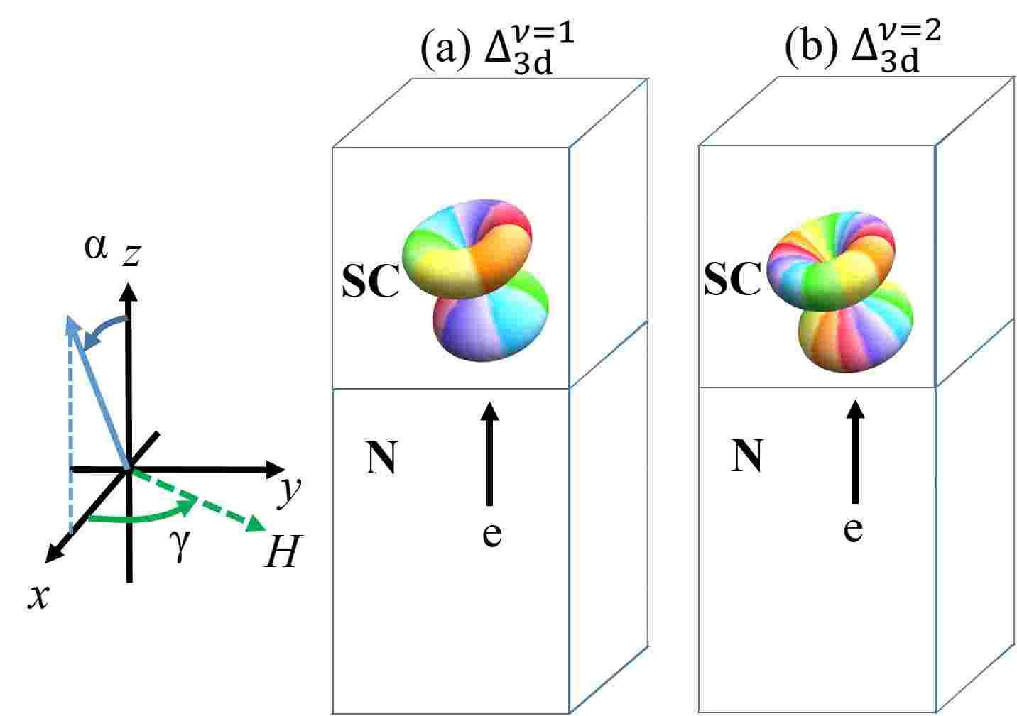
Figure 1: We mainly consider above two types of normal (N) –superconductor (SC) junctions. Here, $\alpha$ is the misorientation angle from the $k_{z}$-axis. Magnetic field is applied in the $x-y$ plane, rotated from the $x$-axis by $\gamma$.

In the following, we explain eight types of pair potentials and corresponding formulae for tunneling conductance and SABS. In Sec. II.1, we explain the case for which the BdG Hamiltonian can be reduced to a $2\times 2$ form [$\Delta_{\mathrm{3d}}^{\nu=0,1,2}$, $\Delta_{\mathrm{2d}}^{\nu=1,2}$, and $\Delta_{E_{1u}}^{\mathrm{chiral}}$]. In Sec. II.2, we explain the case for which the $4\times 4$ BdG Hamiltonian cannot be reduced to two $2\times 2$ blocks [$\Delta_{E_{1u}}^{\mathrm{planar}}$ and $\Delta_{E_{2u}}^{f+p}$]. In Sec. II.3, we briefly summarize the zero-energy SABS (ZESABS) stemming from topological numbers.

II.1 $2\times 2$ BdG Hamiltonian

In this subsection, we introduce pair potentials for 3D and 2D-like chiral superconductors. We derive a formula for the SABS for which the BdG Hamiltonian can be reduced to two $2\times 2$ matrices. $\Delta(\mathbf{k})$ takes

$$\Delta_{3\mathrm{d}}^{\nu}(\mathbf{k})= \left\{\begin{aligned} &\tilde{\Delta}_{\mathrm{3d}}^{\nu}i\sigma_{2}&\nu:\mathrm{odd},\\ &\tilde{\Delta}_{\mathrm{3d}}^{\nu}\sigma_{3}i\sigma_{2}&\nu:\mathrm{even},\\ \end{aligned}\right.$$ (2)

$$\Delta_{2\mathrm{d}}^{\nu}(\mathbf{k})= \left\{\begin{aligned} &\tilde{\Delta}_{\mathrm{2d}}^{\nu}\sigma_{3}i\sigma_{2}&\nu:\mathrm{odd},\\ &\tilde{\Delta}_{\mathrm{2d}}^{\nu}i\sigma_{2}&\nu:\mathrm{even},\end{aligned}\right.$$ (3)

$$\Delta_{E_{1u}}^{\mathrm{chiral}}(\mathbf{k})= \tilde{\Delta}_{E_{1u}}^{\mathrm{chiral}}\sigma_{3}i\sigma_{2},$$ (4)

$$\tilde{\Delta}_{\mathrm{3d}}^{\nu}= \frac{\Delta_{0}}{r_{\mathrm{3d},\nu}k_{\mathrm{F}}^{\nu+1}}k^{\prime}_{z}(k^{\prime}_{x}+ik^{\prime}_{y})^{\nu},$$

$$\tilde{\Delta}_{\mathrm{2d}}^{\nu}= \frac{\Delta_{0}}{k_{\mathrm{F}}^{\nu}}(k^{\prime}_{x}+ik^{\prime}_{y})^{\nu},$$

$$\tilde{\Delta}_{E_{1u}}^{\mathrm{chiral}}= \frac{\Delta_{0}}{r_{E_{1u}}k_{\mathrm{F}}^{3}}\left({5k^{\prime}_{z}}^{2}-k_{\mathrm{F}}^{2}\right)(k^{\prime}_{x}+ik^{\prime}_{y}),$$

$$k^{\prime}_{x}= k_{x}\cos\alpha-k_{z}\sin\alpha,$$

$$k^{\prime}_{y}= k_{y},$$

$$k^{\prime}_{z}= k_{x}\sin\alpha+k_{z}\cos\alpha,$$

where $\alpha$ is the misorientation angle from the $k_{z}$ axis and $(r_{\mathrm{3d},\nu=0},r_{\mathrm{3d},\nu=1},r_{\mathrm{3d},\nu=2},r_{E_{1u}})=(1,\>1/2,\>2/\sqrt{27},\>16/(3\sqrt{15}))$ are the normalization factors so that the maximum value of the pair potential becomes $\Delta_{0}$. Because the direction of the $\mathbf{d}$-vector in spin-space does not affect conductance, $i.e$., conductance is invariant under spin rotation (Appendix C.3), we fix the direction of the $\mathbf{d}$-vector given in Eqs. (2), (3), and (4) for the spin-triplet cases. $\Delta_{\mathrm{3d}}^{\nu}$ and $\Delta_{\mathrm{2d}}^{\nu}$ are chosen in Sec. III.1 and Sec: III.2. We study $\Delta_{\mathrm{3d}}^{\nu=2}$ and $\Delta_{E_{1u}}^{\mathrm{chiral}}$ in Sec. III.3. Under the quasiclassical approximation, the magnitude of the wave vector is pinned to the value on the Fermi surface, $k_{z}=\sqrt{k_{\mathrm{F}}^{2}-k_{x}^{2}-k_{y}^{2}}$. As shown in Fig. 2, $\Delta_{3\mathrm{d}}^{\nu=0}$ has a line node, $\Delta_{3\mathrm{d}}^{\nu}$($\nu=1,2$) has two point nodes and one line node, and $\Delta_{2\mathrm{d}}^{\nu}$ ($\nu>0$) has two point nodes. $\Delta_{E_{1u}}^{\mathrm{chiral}}$ has two point nodes and two line nodes.

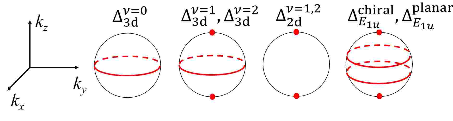
Figure 2: Schematic illustration of nodal structures of $\Delta(\mathbf{k})$ with $\alpha=0$. Red points and lines indicate the positions of nodes.

Then, we show that the BdG Hamiltonian can be reduced to a $2\times 2$ form for all the cases. For the spin-singlet cases ($\Delta_{\mathrm{3d}}^{\nu=1}$ and $\Delta_{\mathrm{2d}}^{\nu=2}$), Eq. (1) is reduced to

$${\cal H}(\mathbf{k})= \frac{1}{2}\sum_{\mathbf{k}}\Psi^{\dagger}(\mathbf{k})\begin{pmatrix}\varepsilon(\mathbf{k})&0&0&D\\ 0&\varepsilon(\mathbf{k})&-D&0\\ 0&-D^{*}&-\varepsilon(\mathbf{k})&0\\ D^{*}&0&0&-\varepsilon(\mathbf{k})\end{pmatrix}\Psi(\mathbf{k})$$

$$= \frac{1}{2}\sum_{\mathbf{k}}(c_{\mathbf{k},\uparrow}^{\dagger}\>c_{-\mathbf{k},\downarrow})\begin{pmatrix}\varepsilon(\mathbf{k})&D\\ D^{*}&-\varepsilon(\mathbf{k})\end{pmatrix}\begin{pmatrix}c_{\mathbf{k},\uparrow}\\ c_{-\mathbf{k}\downarrow}^{\dagger}\end{pmatrix}$$

$$+\frac{1}{2}\sum_{\mathbf{k}}(c_{\mathbf{k},\downarrow}^{\dagger}\>c_{-\mathbf{k},\uparrow})\begin{pmatrix}\varepsilon(\mathbf{k})&-D\\ -D^{*}&-\varepsilon(\mathbf{k})\end{pmatrix}\begin{pmatrix}c_{\mathbf{k},\downarrow}\\ c_{-\mathbf{k}\uparrow}^{\dagger}\end{pmatrix},$$

with $Di\sigma_{2}=\Delta_{\mathrm{3d}}^{\nu=1}$ or $\Delta_{\mathrm{2d}}^{\nu=2}$. For the spin-triplet cases ($\Delta_{\mathrm{3d}}^{\nu=0,2}$, $\Delta_{\mathrm{2d}}^{\nu=1}$, and $\Delta_{E_{1u}}^{\mathrm{chiral}}$), with a $\mathbf{d}$-vector, Eq. (1) becomes

$${\cal H}(\mathbf{k})= \frac{1}{2}\sum_{\mathbf{k}}\Psi^{\dagger}(\mathbf{k})\begin{pmatrix}\varepsilon(\mathbf{k})&0&0&d_{3}\\ 0&\varepsilon(\mathbf{k})&d_{3}&0\\ 0&d_{3}^{*}&-\varepsilon(\mathbf{k})&0\\ d_{3}^{*}&0&0&-\varepsilon(\mathbf{k})\end{pmatrix}\Psi(\mathbf{k})$$

$$= \frac{1}{2}\sum_{\mathbf{k}}(c_{\mathbf{k},\uparrow}^{\dagger}\>c_{-\mathbf{k},\downarrow})\begin{pmatrix}\varepsilon(\mathbf{k})&d_{3}\\ d_{3}^{*}&-\varepsilon(\mathbf{k})\end{pmatrix}\begin{pmatrix}c_{\mathbf{k},\uparrow}\\ c_{-\mathbf{k}\downarrow}^{\dagger}\end{pmatrix}$$

$$+\frac{1}{2}\sum_{\mathbf{k}}(c_{\mathbf{k},\downarrow}^{\dagger}\>c_{-\mathbf{k},\uparrow})\begin{pmatrix}\varepsilon(\mathbf{k})&d_{3}\\ d_{3}^{*}&-\varepsilon(\mathbf{k})\end{pmatrix}\begin{pmatrix}c_{\mathbf{k},\downarrow}\\ c_{-\mathbf{k}\uparrow}^{\dagger}\end{pmatrix},$$

with $(d_{3}\sigma_{3})(i\sigma_{2})=\Delta_{\mathrm{3d}}^{\nu=2}$, $\Delta_{\mathrm{2d}}^{\nu=1}$, or $\Delta_{E_{1u}}^{\mathrm{chiral}}$.

In the following, we calculate the charge conductance by using the extended version Tanaka and Kashiwaya (1995); Kashiwaya and Tanaka (2000); Kashiwaya et al. (1996) of the Blonder–Tinkham–Klapwijk (BTK) formula Blonder et al. (1982) for unconventional superconductors Bruder (1990).

Since we assume that the penetration depth of the magnetic field $\lambda$ is much larger than the coherence length of the pair potential Fogelström et al. (1997); Tanuma et al. (2002b), we can neglect the spatial dependence of the magnetic field. Therefore, we can take the vector potential as

$$\mathbf{A}=(-H\lambda\sin\gamma,H\lambda\cos\gamma,0).$$ (5)

Solving the BdG equation with the quasiclassical approximation, where $\mu$ is much larger than the energy of an injected electron $|eV|$ and $|\Delta(\mathbf{k}_{\parallel})|$, the wave function in the normal metal (N) and superconductor (S) are obtained as

$$\Psi_{\sigma}^{\mathrm{N}}(z<0,\mathbf{k}_{\parallel})= \psi_{e,\sigma}^{\mathrm{N}}e^{i\mathbf{k}\cdot\mathbf{r}}$$

$$+\sum_{\sigma^{\prime}=\pm}\left(a_{\sigma,\sigma^{\prime}}\psi_{h,\sigma^{\prime}}^{\mathrm{N}}e^{i\mathbf{k}\cdot\mathbf{r}}+b_{\sigma,\sigma^{\prime}}\psi_{e,\sigma^{\prime}}^{\mathrm{N}}e^{i\tilde{\mathbf{k}}\cdot\mathbf{r}}\right),$$ (6)

$$\Psi^{\mathrm{S}}(z>0,\mathbf{k}_{\parallel})= \sum_{\sigma^{\prime}=\pm}\left(c_{\sigma^{\prime}}\psi_{e,\sigma^{\prime}}^{\mathrm{S}}e^{i\mathbf{k}\cdot\mathbf{r}}+d_{\sigma^{\prime}}\psi_{h,\sigma^{\prime}}^{\mathrm{S}}e^{i\tilde{\mathbf{k}}\cdot\mathbf{r}}\right),$$ (7)

and

$$\psi_{e,\sigma}^{\mathrm{N}}= (1+\sigma,1-\sigma,0,0)^{\mathrm{T}}/2,$$ (8)

$$\psi_{h,\sigma}^{\mathrm{N}}= (0,0,1+\sigma,1-\sigma)^{\mathrm{T}}/2,$$ (9)

$$\psi_{e,\sigma}^{\mathrm{S}}= [1+\sigma,1-\sigma,(1-\sigma)\rho\Gamma_{+},(1+\sigma)\Gamma_{+}]^{\mathrm{T}}/2,$$

$$\psi_{h,\sigma}^{\mathrm{S}}= [(1+\sigma)\Gamma_{-},(1-\sigma)\rho\Gamma_{-},1-\sigma,1+\sigma]^{\mathrm{T}}/2,$$

$$\Gamma_{+}= \frac{\Delta^{*}(\mathbf{k})}{\tilde{E}+\sqrt{\tilde{E}^{2}-|\Delta(\mathbf{k})|^{2}}},$$ (10)

$$\Gamma_{-}= \frac{\Delta(\tilde{\mathbf{k}})}{\tilde{E}+\sqrt{\tilde{E}^{2}-|\Delta(\tilde{\mathbf{k}})|^{2}}},$$ (11)

$$\tilde{E}= eV-\frac{H}{H_{0}}\Delta_{0}\left(\frac{k_{y}}{k_{\mathrm{F}}}\cos\gamma-\frac{k_{x}}{k_{\mathrm{F}}}\sin\gamma\right),$$ (12)

with $\tilde{\mathbf{k}}=(k_{x},k_{y},-k_{z})$ and $H_{0}=\Delta_{0}/(e\lambda v_{\mathrm{F}})$. $\Delta(\mathbf{k})=\tilde{\Delta}_{\mathrm{3d}}^{\nu}(\mathbf{k})$, $\tilde{\Delta}_{\mathrm{2d}}^{\nu}(\mathbf{k})$, or $\tilde{\Delta}_{E_{1u}}^{\mathrm{chiral}}(\mathbf{k})$. Here, $\rho=-1$ for $\Delta_{3\mathrm{d}}^{\nu=1}$ and $\Delta_{2\mathrm{d}}^{\nu=2}$ (even parity) and $\rho=1$ for $\Delta_{3\mathrm{d}}^{\nu=0,2}$, $\Delta_{2\mathrm{d}}^{\nu=1}$, and $\Delta_{E_{1u}}^{\mathrm{chiral}}$ (odd parity). The coefficients ($a_{\sigma,\sigma^{\prime}},b_{\sigma,\sigma^{\prime}},c_{\sigma},d_{\sigma}$) are determined by the boundary conditions:

$$\Psi_{\sigma}^{\mathrm{N}}(0_{-},\mathbf{k}_{\parallel})= \Psi^{\mathrm{S}}(0_{+},\mathbf{k}_{\parallel}),$$ (13)

$$\left.\frac{d\Psi^{\mathrm{S}}}{dz}\right|_{z=0_{+}}-\left.\frac{d\Psi^{\mathrm{N}}_{\sigma}}{dz}\right|_{z=0_{-}}= \frac{2mU_{0}}{\hbar^{2}}\Psi^{\mathrm{N}}_{\sigma}(0_{-},\mathbf{k}_{\parallel}),$$ (14)

where the insulating barrier at $z=0$ is simplified as $V(z)=U_{0}\delta(z)$. The angle-resolved conductance is given by Tanaka and Kashiwaya (1995); Kashiwaya et al. (1996)

$$\sigma_{\mathrm{S}}(eV,\mathbf{k}_{\parallel})= 1+\frac{1}{2}\sum_{\sigma,\sigma^{\prime}=\pm}\left[|a_{\sigma,\sigma^{\prime}}|^{2}-|b_{\sigma,\sigma^{\prime}}|^{2}\right]$$

$$= \sigma_{\mathrm{N}}\frac{1+\sigma_{\mathrm{N}}|\Gamma_{+}|^{2}+(\sigma_{\mathrm{N}}-1)|\Gamma_{+}\Gamma_{-}|^{2}}{|1+(\sigma_{\mathrm{N}}-1)\Gamma_{+}\Gamma_{-}|^{2}},$$ (15)

$$\sigma_{\mathrm{N}}(\mathbf{k}_{\parallel})= \frac{4\cos^{2}\theta}{4\cos^{2}\theta+Z^{2}},$$ (16)

with $\cos\theta=k_{z}/k_{\mathrm{F}}$ and $Z=2mU_{0}/(\hbar^{2}k_{\mathrm{F}})$.

In the procedure of obtaining conductance with magnetic field, we neglect Zeeman effect. For UPt₃, the order of $\lambda\sim 10^{4}$ÅBroholm et al. (1990) $k_{\mathrm{F}}\sim 1/$ÅMarabelli et al. (1986). Here the order of the energy of Doppler shift is $H\Delta/H_{0}$ with $H_{0}=h/(2e\pi^{2}\xi\lambda)$ and $\xi=\hbar^{2}k_{\mathrm{F}}/(\pi m\Delta)$ Fogelström et al. (1997). Since the Zeeman energy is given by $\mu_{B}H$, the ratio of the energy of Doppler shift to Zeeman effect is $2\lambda k_{\mathrm{F}}\sim 10^{4}$ times larger than that of Zeeman energy for UPt₃. Thus, neglecting Zeeman effect is a good approximation in present case.

In Sec. III.1, we discuss SABSs with $H=0$, which is determined by requiring the condition that the denominator of Eq. (15) is zero for $Z\rightarrow\infty$ ($\sigma_{\mathrm{N}}\rightarrow 0$). Then, at the energy dispersion of the SABS, the denominator of Eq. (15) must satisfy following conditions:

$$\mathrm{Re}(\Gamma_{+}\Gamma_{-})= 1,$$ (17)

$$\mathrm{Im}(\Gamma_{+}\Gamma_{-})= 0.$$ (18)

In this case, $\sigma_{\mathrm{S}}$ becomes two, which is the maximum value of angle-resolved conductance owing to the perfect resonance. We define $E(\mathbf{k}_{\parallel})=\tilde{E}$, which satisfies Eq. (17) and Eq. (18).

Here, we derive a general formula of SABS for pair potentials with arbitrary momentum dependence (details are explained in Appendix B). There are two cases. For $\mathrm{Im}\left[\Delta^{*}(\mathbf{k})\Delta(\tilde{\mathbf{k}})\right]\neq 0$, the energy dispersion of SABS $E(\mathbf{k}_{\parallel})$ is given by

$$E(\mathbf{k}_{\parallel}) =\frac{\mathrm{Im}\left[\Delta^{*}(\mathbf{k})\Delta(\tilde{\mathbf{k}})\right]}{\left|\Delta(\mathbf{k})-\Delta(\tilde{\mathbf{k}})\right|}$$ (19)

where $\Delta(\mathbf{k})$ and $\Delta(\tilde{\mathbf{k}})$ must satisfy

$$\left\{\left|\Delta(\mathbf{k})\right|^{2}-\mathrm{Re}\left[\Delta^{*}(\mathbf{k})\Delta(\tilde{\mathbf{k}})\right]\right\}$$

$$\times\left\{\left|\Delta(\tilde{\mathbf{k}})\right|^{2}-\mathrm{Re}\left[\Delta^{*}(\mathbf{k})\Delta(\tilde{\mathbf{k}})\right]\right\}\geq 0.$$ (20)

For $\mathrm{Im}\left[\Delta^{*}(\mathbf{k})\Delta(\tilde{\mathbf{k}})\right]=0$,

$$E(\mathbf{k}_{\parallel})= 0,$$ (21)

$$\mathrm{with}\>\frac{\Delta(\mathbf{k})}{|\Delta(\mathbf{k})|}= -\frac{\Delta(\tilde{\mathbf{k}})}{|\Delta(\tilde{\mathbf{k}})|}.$$ (22)

This formula reproduces all of the known results of SABSs in 2D unconventional superconductors, such as $d$-wave Hu (1994); Kashiwaya and Tanaka (2000), $p$-wave Hara and Nagai (1986); Kwon et al. (2004), $d+is$-wave Matsumoto and Shiba (1995); Kashiwaya et al. (1995b), chiral $p$-wave Furusaki et al. (2001), and chiral $d$-wave.

In Sec. III.2 and Sec. III.3, we discuss the normalized conductance given by

$$\sigma(eV)=\frac{\int_{|k_{x}^{2}+k_{y}^{2}|<k_{\mathrm{F}}}dk_{x}dk_{y}\sigma_{\mathrm{S}}(eV,k_{x},k_{y})}{\int_{|k_{x}^{2}+k_{y}^{2}|<k_{\mathrm{F}}}dk_{x}dk_{y}\sigma_{\mathrm{N}}(k_{x},k_{y})},$$ (23)

which can be measured experimentally Kashiwaya and Tanaka (2000).

II.2 $4\times 4$ BdG Hamiltonian

In this subsection, we explain the case in which the BdG Hamiltonian is in the $4\times 4$ form. In Sec. III.3, in addition to $\Delta_{\mathrm{3d}}^{\nu=2}$ and $\Delta_{E_{1u}}^{\mathrm{chiral}}$, we choose $\Delta_{E_{1u}}^{\mathrm{planar}}$ (Fig. 2) and $\Delta_{E_{2u}}^{f+p}$. $\Delta_{E_{1u}}^{\mathrm{planar}}$ is a spin-triplet pair potential in a unitary state $i.e$. $\mathbf{q}=i\mathbf{d}\times\mathbf{d}^{*}=0$, while $\Delta_{E_{2u}}^{f+p}$ can incorporate non-unitary case ($\mathbf{q}\neq 0$). $\Delta_{E_{1u}}^{\mathrm{planar}}$ is given by

$$\Delta_{E_{1u}}^{\mathrm{planar}}(\mathbf{k})= \frac{\Delta_{0}}{r_{E_{1u}}k_{\mathrm{F}}^{3}}\left({5k^{\prime}_{z}}^{2}-k_{\mathrm{F}}^{2}\right)(ik^{\prime}_{x}\sigma_{0}+k^{\prime}_{y}\sigma_{1}).$$ (24)

It is noted that the time reversal symmetry is not broken for $\Delta_{E_{1u}}^{\mathrm{planar}}$ but $\Delta_{E_{1u}}^{\mathrm{chiral}}$ does not have time reversal symmetry.

$\Delta_{E_{2u}}^{f+p}$ is the combination of chiral $p$-wave and $f$-wave pairings. The $\mathbf{d}$-vector of $\Delta_{E_{2u}}^{f+p}$ is given by

$$\mathbf{d}= \frac{\Delta_{0}}{r^{f+p}}\left\{\delta\frac{1}{k_{\mathrm{F}}}\left[\left(k^{\prime}_{x}+i\eta k^{\prime}_{y}\right)d_{x}+i\left(\eta k^{\prime}_{x}+ik^{\prime}_{y}\right)d_{y}\right]\right.$$

$$+\left.\frac{1}{k_{\mathrm{F}}^{3}}\left[k^{\prime}_{z}({k^{\prime}_{x}}^{2}-{k^{\prime}_{y}}^{2})+2i\eta k^{\prime}_{z}k^{\prime}_{x}k^{\prime}_{y}\right]d_{z}\right\},$$ (25)

where $\delta$ is considered to be small Yanase (2016) and $r^{f+p}$ is a normalized factor that is determined numerically so that the maximum value of the pair potential becomes $\Delta_{0}$. If $(\eta,\delta)=(1,0)$ is satisfied, we obtain $\Delta_{E_{2u}}^{f+p}=\Delta_{\mathrm{3d}}^{\nu=2}$. The position of nodes of this $f$+$p$-wave pairing depends on the values of $\eta$ and $\delta$. If $\delta=0$ is satisfied (Fig. 3), there are two cases. In the case of $\eta=0$ [Fig. 3 (a-i)–(a-iii)], there are three line nodes. For $\eta>0$ [Fig. 3 (b-i)–(b-iii)], there is a line node and two point nodes. For $\delta>0$ (Fig. 4), there are three cases. For $\eta<1$ [Fig. 4 (a-i)–(a-iii)], there are 16 point nodes on $k_{y}=\pm k_{x}$ lines [Fig. 4 (a-ii)]. In the case of $\eta=1$ [Fig. 4 (b-i)–(b-iii)], the positions of nodes are the same as that in the case of $\eta>0$ and $\delta=0$ [Fig. 3 (b-i)–(b-iii)]. For $\eta>1$ [Fig. 4 (c-i)–(c-iii)], there are 16 point nodes on lines $k_{x}k_{y}=0$, as shown in Fig. 4 (c-ii).

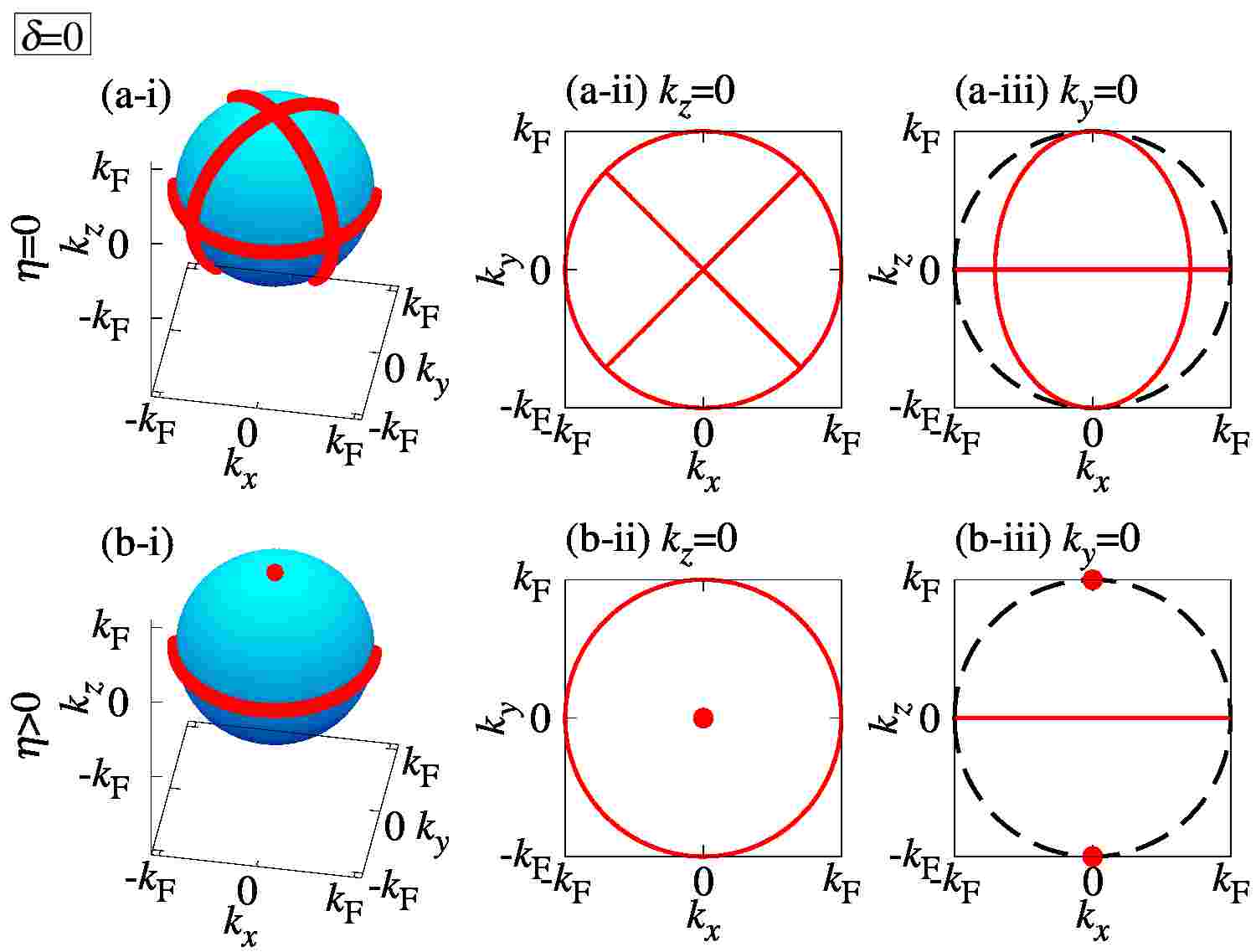
Figure 3: Red lines and dots indicate the positions of nodes of the pair potentials $\Delta_{E_{2u}}^{f+p}$ for $\delta=0$. $\eta=0$ for (a-i)–(a-iii). $\eta>0$ for (b-i)–(b-iii). (a-ii) and (b-ii) are nodes projected on the $k_{z}=0$ plane. (a-iii) and (b-iii) are nodes projected on the $k_{y}=0$ plane. Dashed lines in (a-iii) and (b-iii) indicate projected Fermi surface on $k_{y}=0$ plane.

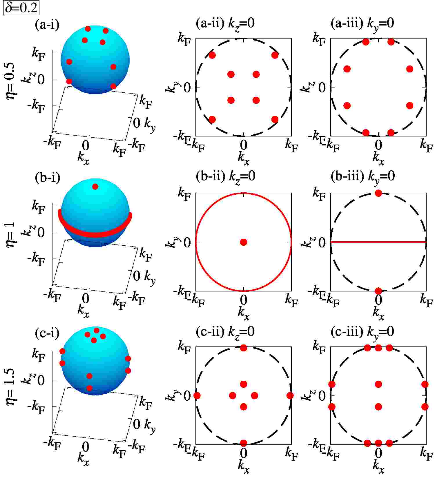
Figure 4: Red lines and dots indicate the positions of nodes of the pair potential $\Delta_{E_{2u}}^{f+p}$ for $\delta=0.2$. $\eta=0.5$ for (a-i)–(a-iii). $\eta=1$ for (b-i)–(b-iii). $\eta=1.5$ for (c-i)–(c-iii). (a-ii), (b-ii), and (c-ii) are nodes projected on the $k_{z}=0$ plane. (a-iii), (b-iii), and (c-iii) are nodes projected on the $k_{y}=0$ plane. Dashed lines in (a-ii), (a-iii), (b-iii), (c-ii), and (c-iii) indicate the projected Fermi surface on the $k_{z}=0$ or $k_{y}=0$ plane.

The wave function for the normal metal side is shown in Eq. (6) with Eq. (8) and Eq. (9) and that for the superconducting side is given in Eq. (7) with

$$\begin{pmatrix}\psi_{e,\uparrow}^{\mathrm{S}}&\psi_{e,\downarrow}^{\mathrm{S}}&\psi_{h,\uparrow}^{\mathrm{S}}&\psi_{h,\downarrow}^{\mathrm{S}}\end{pmatrix}= \begin{pmatrix}u_{e}&v_{h}\\ v_{e}&u_{h}\end{pmatrix},$$

with

$$u_{e(h)}= \frac{[\tilde{E}+\omega_{+(-)}]\sigma_{0}}{\sqrt{(\tilde{E}+\omega_{+(-)})^{2}+\frac{1}{2}\mathrm{Tr}\Delta_{+(-)}\Delta_{+(-)}^{\dagger}}},$$

$$v_{e}= \frac{\Delta_{+}^{\dagger}}{\sqrt{(\tilde{E}+\omega_{+})^{2}+\frac{1}{2}\mathrm{Tr}\Delta_{+}\Delta_{+}^{\dagger}}},$$

$$v_{h}= \frac{\Delta_{-}}{\sqrt{(\tilde{E}+\omega_{-})^{2}+\frac{1}{2}\mathrm{Tr}\Delta_{-}\Delta_{-}^{\dagger}}},$$

$$\omega_{\pm}= \sqrt{\tilde{E}^{2}-\frac{1}{2}\mathrm{Tr}\Delta_{\pm}\Delta_{\pm}^{\dagger}},$$

$$\Delta_{+}= \Delta_{E_{1u}}^{\mathrm{planar}}(\mathbf{k}),$$

$$\Delta_{-}= \Delta_{E_{1u}}^{\mathrm{planar}}(\tilde{\mathbf{k}}),$$

for $\Delta_{E_{1u}}^{\mathrm{planar}}(\mathbf{k})$ and

$$u_{e}= a_{+}[|\mathbf{q}_{+}|\sigma_{0}+\mathbf{q}_{+}\cdot\boldsymbol{\sigma}](\sigma_{0}+\sigma_{3})$$

$$+b_{+}[|\mathbf{q}_{+}|\sigma_{0}-\mathbf{q}_{+}\cdot\boldsymbol{\sigma}](\sigma_{0}-\sigma_{3}),$$

$$u_{h}= a_{-}[|\mathbf{q}_{-}|\sigma_{0}+\mathbf{q}_{-}\cdot\boldsymbol{\sigma}^{*}](\sigma_{0}+\sigma_{3})$$

$$+b_{-}[|\mathbf{q}_{-}|\sigma_{0}-\mathbf{q}_{-}\cdot\boldsymbol{\sigma}^{*}](\sigma_{0}-\sigma_{3}),$$

$$a_{\pm}= \frac{1}{\sqrt{16|\mathbf{q}_{\pm}|[|\mathbf{q}_{\pm}|+(\mathbf{q}_{\pm})_{3}]}}\sqrt{\frac{\tilde{E}+\omega_{\pm,p}}{\tilde{E}}},$$

$$b_{\pm}= \frac{1}{\sqrt{16|\mathbf{q}_{\pm}|[|\mathbf{q}_{\pm}|+(\mathbf{q}_{\pm})_{3}]}}\sqrt{\frac{\tilde{E}+\omega_{\pm,m}}{\tilde{E}}},$$

$$v_{e}= \Delta_{+}^{\dagger}u_{e}(\tilde{E}\sigma_{0}+\hat{\omega}_{+,pm})^{-1},$$

$$v_{h}= \Delta_{-}u_{h}(\tilde{E}\sigma_{0}+\hat{\omega}_{-,pm})^{-1},$$

$$\hat{\omega}_{\pm,pm}= \begin{pmatrix}\omega_{\pm,p}&0\\ 0&\omega_{\pm,m}\end{pmatrix},$$

$$\omega_{\pm,p}= \sqrt{\tilde{E}^{2}-(|\mathbf{d}_{\pm}|^{2}+|\mathbf{q_{\pm}}|)},$$

$$\omega_{\pm,m}= \sqrt{\tilde{E}^{2}-(|\mathbf{d}_{\pm}|^{2}-|\mathbf{q_{\pm}}|)},$$

$$\mathbf{q}_{\pm}= i\mathbf{d}_{\pm}\times\mathbf{d}^{*}_{\pm},$$

$$\mathbf{d}_{+}= \mathbf{d}(\mathbf{k}),$$

$$\mathbf{d}_{-}= \mathbf{d}(\tilde{\mathbf{k}}),$$

for $\Delta_{E_{2u}}^{f+p}$. The boundary conditions are given in Eq. (13) and Eq. (14). We derive a general formula for conductance, which includes the non-unitary case. This formula is similar to that derived in the context of doped topological insulators Takami et al. (2014). In the present case, $\Gamma_{\pm}$ is available for a general pair potential, including non-unitary spin-triplet pairing. The derivation of conductance for a general pair potential is given in Appendix C.

$$\sigma_{\mathrm{S}}= \frac{\sigma_{\mathrm{N}}}{2}\mathrm{Tr}\left[\sigma_{0}-(1-\sigma_{\mathrm{N}})\hat{\Gamma}_{+}^{\dagger}\hat{\Gamma}_{-}^{\dagger}\right]^{-1}$$

$$\times\left[1+\sigma_{\mathrm{N}}\hat{\Gamma}_{+}^{\dagger}\hat{\Gamma}_{+}+(\sigma_{\mathrm{N}}-1)\ \hat{\Gamma}_{+}^{\dagger}\hat{\Gamma}_{-}^{\dagger}\hat{\Gamma}_{-}\hat{\Gamma}_{+}\right]$$

$$\times\left[\sigma_{0}-(1-\sigma_{\mathrm{N}})\hat{\Gamma}_{-}\hat{\Gamma}_{+}\right]^{-1},$$ (26)

with

$$\hat{\Gamma}_{+}= \frac{\Delta_{+}^{\dagger}}{\tilde{E}+\omega_{+}},$$

$$\hat{\Gamma}_{-}= \frac{\Delta_{-}}{\tilde{E}+\omega_{-}},$$

for $\Delta_{E_{1u}}^{\mathrm{planar}}$, and

$$\hat{\Gamma}_{+}= \frac{\Delta_{+}^{\dagger}}{2}\left[\left(\frac{1}{\tilde{E}+\omega_{+,p}}+\frac{1}{\tilde{E}+\omega_{+,m}}\right)\right.$$

$$\left.+\left(\frac{1}{\tilde{E}+\omega_{+,p}}-\frac{1}{\tilde{E}+\omega_{+,m}}\right)\frac{\mathbf{q_{+}}}{|\mathbf{q_{+}}|}\cdot\boldsymbol{\sigma}\right],$$

$$\hat{\Gamma}_{-}= \frac{\Delta_{-}}{2}\left[\left(\frac{1}{\tilde{E}+\omega_{-,p}}+\frac{1}{\tilde{E}+\omega_{-,m}}\right)\right.$$

$$\left.+\left(\frac{1}{\tilde{E}+\omega_{-,p}}-\frac{1}{\tilde{E}+\omega_{-,m}}\right)\frac{\mathbf{q_{-}}}{|\mathbf{q_{-}}|}\cdot\boldsymbol{\sigma}^{*}\right],$$

for $\Delta_{E_{2u}}^{f+p}$. It is noted that the charge conductance for $\Delta_{E_{1u}}^{\mathrm{planar}}$ can be written by using $\Delta_{E_{1u}}^{\mathrm{chiral}}$.

$$\sigma_{\mathrm{S}}(eV,\mathbf{k}_{\parallel})= \frac{\sigma_{\mathrm{N}}}{2}\left[1+\sigma_{\mathrm{N}}|\Gamma_{+}|^{2}+(\sigma_{\mathrm{N}}-1)|\Gamma_{+}\Gamma_{-}|^{2}\right]$$

$$\times\left(\frac{1}{S_{1}}+\frac{1}{S_{2}}\right),$$ (27)

$$S_{1}= \frac{1}{|1+(\sigma_{\mathrm{N}}-1)\Gamma_{+}\Gamma_{-}|^{2}},$$ (28)

$$S_{2}= \frac{1}{|1+(\sigma_{\mathrm{N}}-1)\Omega_{+}\Omega_{-}|^{2}},$$ (29)

$$\Omega_{+}= \frac{\tilde{\Delta}_{E_{1u}}^{\mathrm{chiral}}(\mathbf{k})}{\tilde{E}+\sqrt{\tilde{E}^{2}-|\tilde{\Delta}_{E_{1u}}^{\mathrm{chiral}}(\mathbf{k})|^{2}}},$$

$$\Omega_{-}= \frac{[\tilde{\Delta}_{E_{1u}}^{\mathrm{chiral}}(\tilde{\mathbf{k}})]^{*}}{\tilde{E}+\sqrt{\tilde{E}^{2}-|\tilde{\Delta}_{E_{1u}}^{\mathrm{chiral}}(\tilde{\mathbf{k}})|^{2}}},$$

where $\Gamma_{\pm}$ in Eq. (28) is the same as in Eq. (10) and Eq. (11) if $\Delta$ is replaced by $\tilde{\Delta}_{E_{1u}}^{\mathrm{chiral}}$. SABS is given by Eq. (17), Eq. (18), and

$$\mathrm{Re}(\Omega_{+}\Omega_{-})= 1,$$

$$\mathrm{Im}(\Omega_{+}\Omega_{-})= 0.$$

Owing to the presence of time reversal symmetry, the energy dispersion of the SABS is given by

$$E(\mathbf{k}_{\parallel})=\pm E^{\mathrm{chiral}}(\mathbf{k}_{\parallel}),$$

where $E^{\mathrm{chiral}}(\mathbf{k}_{\parallel})$ is the energy dispersion of the SABS for $\Delta_{E_{1u}}^{\mathrm{chiral}}$. The normalized conductance is given in Eq. (23).

II.3 Topological number

In this subsection, we briefly summarize the main discussion about the number of the ZESABSs for $\Delta_{\mathrm{2d}}^{\nu}$ and $\Delta_{\mathrm{3d}}^{\nu}$ ($\nu\leq 2$) Kobayashi et al. (2015). This result is used in Sec. III.1. The ZESABSs for $\Delta_{\mathrm{2d}}^{\nu}$ are understood only from a 2D topological number (Chern number) and those for $\Delta_{\mathrm{3d}}^{\nu}$ are understood from a one-dimensional topological number (winding number) and the Chern number. Similar discussions for $\Delta_{\mathrm{3d}}^{\nu>2}$ and $\Delta_{E_{1u}}^{\mathrm{chiral}}$ are given in Appendix A. For $\Delta_{\mathrm{3d}}^{\nu>2}$ with $0<\alpha<\pi/4$, cylindrical cuts must be used to calculate the Chern number.

Generally, if a Hamiltonian possesses time reversal symmetry, the winding number can be defined by using a chiral operator $\Gamma=-iCT$ ($C=\sigma_{0}\tau_{1}K$: Charge conjugation, $T=i\sigma_{2}\tau_{0}K$: Time reversal. $\sigma_{i}$ and $\tau_{i}$ are the Pauli matrices in spin and Nambu spaces, respectively,) which anticommutes with the Hamiltonian. The winding number is given by Sato et al. (2011b); Schnyder and Ryu (2011),

$$W(\mathbf{k}_{\parallel},\Gamma)=\frac{-1}{4\pi i}\int_{-\infty}^{\infty}dk_{\perp}\mathrm{Tr}\left[\Gamma H^{-1}(\mathbf{k})\partial_{k_{\perp}}H(\mathbf{k})\right],$$

where $\mathbf{k}_{\parallel}$ and $k_{\perp}$ are wave vectors parallel and perpendicular to a certain surface, respectively. Although $\Delta_{\mathrm{3d}}^{\nu}$ ($\nu\geq 1$) does not have time reversal symmetry, the BdG Hamiltonian hosts a momentum-dependent pseudo time reversal symmetry Kobayashi et al. (2015):

$$U_{\varphi_{\mathbf{k}}}^{\dagger}TU_{\varphi_{\mathbf{k}}}H(\mathbf{k})U_{\varphi_{\mathbf{k}}}^{\dagger}T^{\dagger}U_{\varphi_{\mathbf{k}}}=H(-\mathbf{k}),$$

with $U_{\varphi_{\mathbf{k}}}=\exp(-i\nu\varphi_{\mathbf{k}}\sigma_{0}\tau_{3}/2)$ and $\varphi_{\mathbf{k}}=\tan^{-1}(k_{y}/k_{x})$. Replacing $\Gamma$ with $\Gamma_{\varphi_{\mathbf{k}}}$, we can define the winding number where $\Gamma_{\varphi_{\mathbf{k}}}$ is given by

$$\Gamma_{\varphi_{\mathbf{k}}}=\left\{\begin{aligned} &U_{\varphi_{\mathbf{k}}}^{\dagger}\Gamma U_{\varphi_{\mathbf{k}}}&\>(\nu:\>\mathrm{odd}),\\ &U_{\varphi_{\mathbf{k}}}^{\dagger}S_{z}CTU_{\varphi_{\mathbf{k}}}&\>(\nu:\>\mathrm{even}),\end{aligned}\right.$$

with $S_{z}=\sigma_{3}\tau_{3}$.

The Chern number Thouless et al. (1982) at a fixed $k_{\parallel,1}$ is defined by

$$N(k_{\parallel,1})=\frac{i}{2\pi}\sum_{n\in\mathrm{occ}}\int_{\mathrm{BZ}}dk_{\perp}dk_{\parallel,2}\epsilon^{ab}\partial_{k_{a}}\langle u_{n}(\mathbf{k})|\partial_{k_{b}}|u_{n}(\mathbf{k})\rangle,$$

where $|u_{n}(\mathbf{k})\rangle$ is an eigenstate of $H(\mathbf{k})$ and the summation is taken over all of the occupied states.

These topological numbers connect the number of the ZESABSs by the bulk-boundary correspondence. We show the angle-resolved zero voltage conductance calculated by using Eq. (15) in Fig. 5 ($\Delta_{\mathrm{2d}}^{\nu}$), Fig. 6 ($\Delta_{\mathrm{3d}}^{\nu=0}$), and Fig. 7 ($\Delta_{\mathrm{3d}}^{\nu=1,2}$). The corresponding energy dispersion of SABS calculated by using Eq. (19)–(22) are also shown in the same figures and we discuss them in Sec. III.1.

Table 1: Origin of ZESABSs for each pair potential. $w$ and $c$ indicate winding number and Chern number, respectively.

$\Delta$	$\alpha=0$	$0<\alpha<\frac{\pi}{4}$	$\alpha=\frac{\pi}{4}$	$\frac{\pi}{4}<\alpha<\frac{\pi}{2}$	$\alpha=\frac{\pi}{2}$
$\Delta_{\mathrm{2d}}^{\nu}$	$-$	$c$	$c$	$c$	$c$
$\Delta_{\mathrm{3d}}^{\nu=0}$	$w$	$w$	$w$	$w$	$-$
$\Delta_{\mathrm{3d}}^{\nu=1}$	$w$	$w$	$-$	$c$	$c$
$\Delta_{\mathrm{3d}}^{\nu=2}$	$w$	$w$	$w$	$w$ and $c$	$c$

The position of a line node or point nodes or both on the Fermi surface for each pair potential are shown in Fig. 5 (a-i)–(a-iii), Fig. 6 (b-i)–(b-v), and Fig. 7 (a-i)–(a-v), and those projected on the $k_{x}-k_{y}$ (001) plane are shown in Fig. 5 (b-i)–(b-iii), Fig. 6 (c-i)–(c-v), and Fig. 7 (b-i)–(b-v). For $\Delta_{3d}^{\nu}$, the position of a projected line node is given by

$$\frac{k_{x}^{2}}{\cos^{2}\alpha}+k_{y}^{2}=k_{\mathrm{F}}^{2}.$$ (30)

The ZESABSs, including the spin degrees of freedom for $\Delta_{\mathrm{3d}}^{\nu=0}$, are shown in Fig. 6 (d-i)–(d-v). The angle-resolved conductance at zero bias voltage reflects on the ZESABSs. They are shown in Fig. 5 (d-i)–(d-iii) for $\Delta_{\mathrm{2d}}^{\nu=1}$ and Fig. 5 (g-i)–(g-iii) for $\Delta_{\mathrm{2d}}^{\nu=2}$. They are also shown in Fig. 7 (d-i)–(d-v) for $\Delta_{\mathrm{3d}}^{\nu=1}$ and Fig. 7 (g-i)–(g-v) for $\Delta_{\mathrm{3d}}^{\nu=2}$.

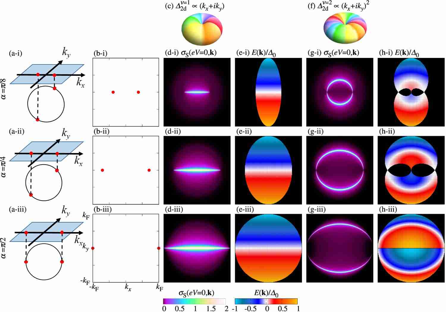
Figure 5: Schematic illustration of point nodes (red dots) for (a-i) $\alpha=\pi/8$, (a-ii) $\alpha=\pi/4$, and (a-iii) $\alpha=\pi/2$. Point nodes projected on the $k_{x}-k_{y}$ plane corresponding to (a-i)–(a-iii) are shown in (b-i)–(b-iii). Schematic picture of pair potential for (c) $\Delta_{2\mathrm{d}}^{\nu=1}$ and (f) $\Delta_{2\mathrm{d}}^{\nu=2}$. The angle-resolved zero bias conductance $\sigma_{\mathrm{S}}(eV=0,\mathbf{k}_{\parallel})$ at $Z=6$ are plotted as functions of $k_{x}$ and $k_{y}$ for $\Delta_{2\mathrm{d}}^{\nu=1}$ (d-i) $\alpha=\pi/8$, (d-ii) $\alpha=\pi/4$, and (d-iii) $\alpha=\pi/2$. Similar plots for $\Delta_{2\mathrm{d}}^{\nu=2}$ for (g-i) $\alpha=\pi/8$, (g-ii) $\alpha=\pi/4$, and (g-iii) $\alpha=\pi/2$. The energy dispersions of the SABS $E(\mathbf{k}_{\parallel})$ are plotted as functions of $k_{x}$ and $k_{y}$ for $\Delta_{2\mathrm{d}}^{\nu=1}$ [(e-i)–(e-iii)] and for $\Delta_{2\mathrm{d}}^{\nu=2}$ [(h-i)–(h-iii)].

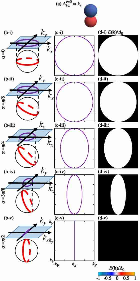
Figure 6: Schematic illustration of pair potential for (a) $\Delta_{3\mathrm{d}}^{\nu=0}$. Schematic illustration of a line node (red line) for (b-i) $\alpha=0$, (b-ii) $\alpha=\pi/8$, (b-iii) $\alpha=\pi/4$, (b-iv) $\alpha=3\pi/8$, and (b-v) $\alpha=\pi/2$. The line node projected on the $k_{x}-k_{y}$ plane corresponding to (b-i)–(b-v) are shown in (c-i)–(c-v). The energy dispersion of SABS $E(\mathbf{k}_{\parallel})$ for given $\alpha$ are plotted as functions of $k_{x}$ and $k_{y}$ [(d-i)–(d-v)].

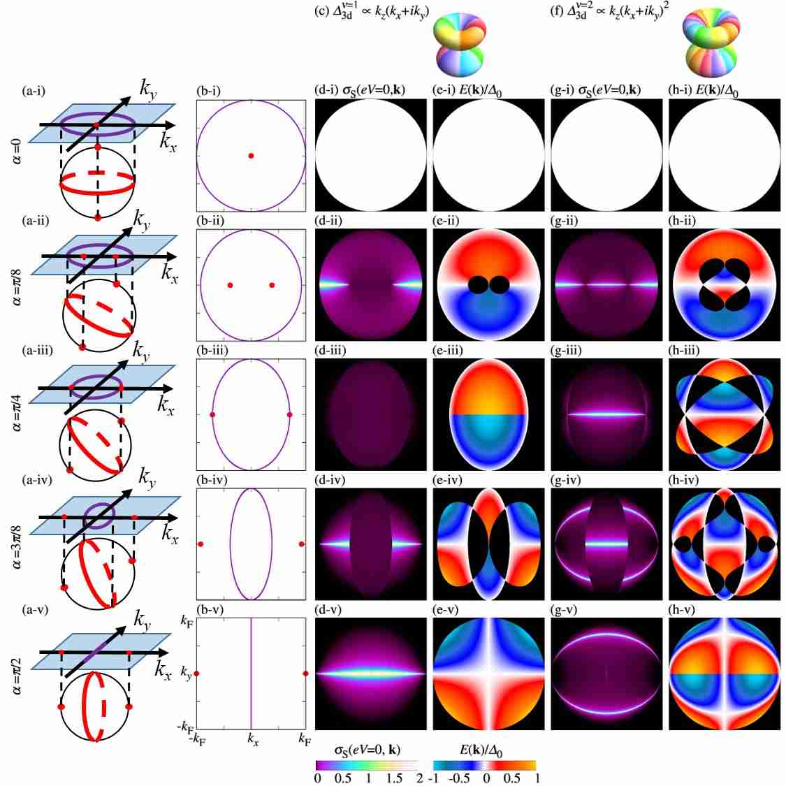
Figure 7: Schematic illustration of point nodes (red dots) and a line node (red line) for (a-i) $\alpha=0$, (a-ii) $\alpha=\pi/8$, (a-iii) $\alpha=\pi/4$, (a-iv) $\alpha=3\pi/8$, and (a-v) $\alpha=\pi/2$. Point nodes and a line node projected on the $k_{x}-k_{y}$ plane corresponding to (a-i)–(a-v) are shown in (b-i)–(b-v). Schematic illustration of pair potential for (c) $\Delta_{3\mathrm{d}}^{\nu=1}$ and (f) $\Delta_{3\mathrm{d}}^{\nu=2}$. The angle-resolved zero bias conductance $\sigma_{\mathrm{S}}(eV=0,\mathbf{k}_{\parallel})$ with $Z=6$ is plotted as functions of $k_{x}$ and $k_{y}$ for $\Delta_{3\mathrm{d}}^{\nu=1}$ [(d-i)–(d-v)] and for $\Delta_{3\mathrm{d}}^{\nu=2}$ [(g-i)–(g-v)]. The energy dispersion of the SABS $E(\mathbf{k}_{\parallel})$ for given $\alpha$ are plotted as functions of $k_{x}$ and $k_{y}$ for $\Delta_{3\mathrm{d}}^{\nu=1}$ [(e-i)–(e-v)] and for $\Delta_{3\mathrm{d}}^{\nu=2}$ [(h-i)–(h-v)].

In the case of $\Delta_{\mathrm{3d}}^{\nu=0}$, there are flat band SABSs within the ellipse of Eq. (30) originated from the winding number [Fig. 6 (d-i)–(d-v)]. There are two bands due to spin degrees of freedom. For $\Delta_{\mathrm{3d}}^{\nu\geq 1}$ with $\alpha=0$, there are flat band SABSs within $k_{x}^{2}+k_{y}^{2}\leq k_{\mathrm{F}}^{2}$ [See Fig. 7 (d-i) and (g-i)]. The origin of these flat bands is explained from the winding number. On the other hand, there is no ZESABS for $\Delta_{\mathrm{2d}}^{\nu}$ with $\alpha=0$ (not shown). In the case of $\alpha=\pi/4$ for $\Delta_{\mathrm{3d}}^{\nu=1}$ there is no ZESABS [Fig. 7 (d-iii)], while they exist on $k_{y}=0$ for $\alpha=\pi/4$ with $\Delta_{\mathrm{3d}}^{\nu=2}$ [Fig. 7 (g-iii)]. In other cases, (except for $\alpha=0,\pi/4$ for $\Delta_{\mathrm{3d}}^{\nu\geq 1}$ and $\alpha=0$ for $\Delta_{\mathrm{2d}}^{\nu}$), the number of the arc shaped ZESABSs which terminate at projected point nodes on the $k_{x}-k_{y}$ plane is $2\nu$, where two comes from the spin degeneracy [see Fig. 5 (d-i)–(d-iii), (g-i)–(g-iii), and Fig. 7 (d-ii), (d-iv), (d-v), (g-ii), (g-iv), and (g-v)]. For $\Delta_{\mathrm{2d}}^{\nu}$, the number of ZESABSs connecting two projected point nodes is $2\nu$.

In addition to the ZESABSs those terminate at the projected point nodes, the ZESABSs located on $k_{y}=0$ and $\cos\alpha>|k_{x}|$ appear for $\pi/4<\alpha\leq\pi/2$ with $\Delta_{\mathrm{3d}}^{\nu=2}$.

For $0<\alpha<\pi/4$ with $\Delta_{\mathrm{3d}}^{\nu=1,2}$, the ZESABSs are originated from the winding number. For $\pi/4<\alpha<\pi/2$ with $\Delta_{\mathrm{3d}}^{\nu=2}$, the ZESABSs are originated from both the winding number and the Chern number. The ZESABSs for $\Delta_{\mathrm{2d}}^{\nu}$ originate from the Chern number for arbitrary $\alpha$ (Table 1).

III Results

III.1 Andreev bound state with $H=0$

In this subsection, we calculate the energy dispersion of the SABS with $H=0$ for two cases of chiral superconductors where pair potentials are given by $(k^{\prime}_{x}+ik^{\prime}_{y})^{\nu}$ ($\nu=1,2$) and $k^{\prime}_{z}(k^{\prime}_{x}+ik^{\prime}_{y})^{\nu}$ ($\nu=1,2$). Although the ZESABS has been discussed in a previous paper Kobayashi et al. (2015), the energy dispersion of the SABS with nonzero energy has not been clarified at all. To resolve this problem, we calculate the energy spectrum of the SABSs from Eqs. (19) to (22).

Here, we apply this formula for normal metal / 3D chiral superconductor junctions. First, we calculate the energy dispersion and tunneling conductance of the 2D-like chiral superconductor, where the pair potential is given by $\Delta_{\mathrm{2d}}^{\nu}\propto(k^{\prime}_{x}+ik^{\prime}_{y})^{\nu}$. The angle-resolved zero bias conductance and the energy dispersion of SABS are shown in Fig. 5. For $\nu=1$, the angle-resolved zero voltage conductance is plotted from Fig. 5 (d-i) to (d-iii). As explained in Sec. II.3, we can see that the ZESABS appears on the line connecting two point nodes at $k_{y}=0$. The region of the ZESABS spreads with the increase of $\alpha$. The corresponding energy dispersion of the SABS $E(\mathbf{k}_{\parallel})$ is shown in Fig. 5 (e-i)–(e-iii). In this case, we can obtain an analytical formula for the SABS, given by

$$E(\mathbf{k}_{\parallel})=-\Delta_{0}k_{y}/k_{\mathrm{F}}$$ (31)

$$\mathrm{with}\>\> k_{x}^{2}+k_{y}^{2}\sin^{2}\alpha\leq k_{\mathrm{F}}^{2}\sin^{2}\alpha.$$ (32)

The number of SABSs including the zero energy state is two (including the spin degeneracy). For $\nu=2$, two branches of the ZESABS appear as arcs on the $k_{x}-k_{y}$ plane connecting two point nodes as shown from Fig. 5 (g-i) to (g-iii). The length of the arcs increases with the increase of $\alpha$. The corresponding $E(\mathbf{k}_{\parallel})$ is shown from Fig. 5 (h-i) to (h-iii). The number of SABSs including zero energy state is four. Then, we can summarize that the number of SABSs stemming from topological origins, including the ZESABS, is $2\nu$.

Next, we focus on the case of 3D chiral superconductors [$\Delta_{\mathrm{3d}}^{\nu}\propto k^{\prime}_{z}(k^{\prime}_{x}+ik^{\prime}_{y})^{\nu}$, including the $p$-wave case]. In the $p$-wave ($\nu=0$) case, (see Fig. 6), the energy dispersion of the SABS is shown from Fig. 6 (d-i) to (d-v). It is located inside the ellipse given by Eq. (30) and there only appears the ZESABS.

For the $\nu=1$ and $2$ cases, (see Fig. 7), the angle-resolved zero voltage conductance is plotted in Fig. 7 (d-i)–(d-v) for $\nu=1$ and the corresponding energy dispersion of the SABS $E(\mathbf{k}_{\parallel})$ is shown in Fig. 7 (e-i)–(e-v). We can derive an analytical formula of $E(\mathbf{k}_{\parallel})$ for $\alpha=\pi/4$ and $\alpha=\pi/2$ given by

$$E(\mathbf{k}_{\parallel})= -\frac{\Delta_{0}}{2\sqrt{2}r_{\mathrm{3d},\nu=1}}\left(\hat{k}_{x}+\sqrt{1-\hat{k}_{x}^{2}-\hat{k}_{y}^{2}}\right)^{2}$$

$$\times\left(\hat{k}_{x}-\sqrt{1-\hat{k}_{x}^{2}-\hat{k}_{y}^{2}}\right)\mathrm{sgn}(\hat{k}_{y}),$$

$$\mathrm{with}\>\> 2k_{x}^{2}+k_{y}^{2}\leq k_{\mathrm{F}}^{2},$$

where $\hat{k}_{i}=k_{i}/k_{\mathrm{F}}$ ($i=x,y,z$) and

$$E(\mathbf{k}_{\parallel})=-\frac{\Delta_{0}}{r_{\mathrm{3d},\nu=1}}\hat{k}_{y}\mid\hat{k}_{x}\mid,$$

respectively. The number of SABSs $n_{\mathrm{ABS}}$, which includes the ZESABS, is classified by whether $(k_{x},k_{y})$ is inside the ellipse [Eq. (30)] or not. Inside the ellipse, $n_{\mathrm{ABS}}$ becomes two (including the spin degeneracy) for $\alpha<\pi/4$ and zero for $\alpha\geq\pi/4$. On the other hand, outside the ellipse, $n_{\mathrm{ABS}}$ becomes zero for $\alpha\leq\pi/4$ and four for $\alpha>\pi/4$. Besides this SABS with topological origin, inside the ellipse, nonzero non-topologically SABS which does not include the zero-energy state exists.

Next, we focus on the $\nu=2$ case. Angle-resolved zero voltage conductance is plotted in Fig. 7 (g-i)–(g-v) and the corresponding energy dispersion of the SABS $E(\mathbf{k}_{\parallel})$ is shown in Fig. 7 (h-i)–(h-v). We can derive an analytical formula of $E(\mathbf{k}_{\parallel})$ for $\alpha=\pi/2$ given by

$$E(\mathbf{k}_{\parallel})=\frac{\Delta_{0}}{r_{\mathrm{3d},\nu=2}}\mathrm{sgn}(\hat{k}_{y})|\hat{k}_{x}|(1-\hat{k}_{x}^{2}-2\hat{k}_{y}^{2}).$$

$n_{\mathrm{ABS}}$ is also classified whether $(k_{x},k_{y})$ is inside the ellipse or not. Inside the ellipse, $n_{\mathrm{ABS}}$ becomes two for $\alpha=0$. For $0<\alpha<\pi/4$, $n_{\mathrm{ABS}}$ is four and $n_{\mathrm{ABS}}=2$ for $\alpha\geq\pi/4$. On the other hand, outside the ellipse, $n_{\mathrm{ABS}}$ becomes zero for $\alpha\leq\pi/4$ and eight for $\alpha>\pi/4$. Beside this SABS with topological origin, nonzero non-topologically SABSs also exist.

We further calculate $n_{\mathrm{ABS}}$ up to $\nu=4$ (The ZESABSs for $0<\alpha<\pi/4$ with $\nu=3,4$ are discussed in Appendix A.2). A summary of $n_{\mathrm{ABS}}$ as a function of $\nu$ is shown in Table. 2. We can also obtain the analytical formula of $E(\mathbf{k}_{\parallel})$ both for the 3D and 2D-like chiral superconductors for $\alpha=\pi/2$. The results are summarized in Table 3.

Table 2: The number of SABS ($n_{\mathrm{ABS}}$) which cross zero-energy for $\Delta_{\mathrm{3d}}^{\nu}$. It is classified by inside or outside of the ellipse [Eq. (30)] corresponding to projected line node [Fig. 6 (c-i)–(c-v) and Fig. 7 (b-i)–(b-v)]. $n_{\mathrm{ABS}}$ is counted including the spin degeneracy. The dash ”-” means there is no area inside or outside the ellipse [Fig. 6 (c-i) and (c-v)].

	$n_{\mathrm{ABS}}$
$\alpha$	Inside ellipse	Outside ellipse
0	2	$-$
$0<\alpha<\frac{\pi}{4}$	$2\nu$	$0$
$\alpha=\pi/4$	$2(\nu-1)$	$0$
$\frac{\pi}{4}<\alpha<\frac{\pi}{2}$	$2(\nu-1)$	$4\nu$
$\alpha=\pi/2$	$-$	$4\nu$

Table 3: The energy dispersion of SABS $E(\mathbf{k}_{\parallel})/\Delta_{0}$ times normalization factor $r$ ($r=r_{\mathrm{3d},\nu}$ for $\Delta_{\mathrm{3d}}^{\nu}$ and $r=1$ for $\Delta_{\mathrm{2d}}^{\nu}$) at $\alpha=\pi/2$ is shown for $\Delta_{3\mathrm{d}}^{\nu}$ and $\Delta_{2\mathrm{d}}^{\nu}$. $\hat{k}_{i}=k_{i}/k_{\mathrm{F}}(i=x,y,z)$. For the chiral 3D superconductor, the line $k_{x}$=0 does not express the energy dispersion of SABS since $\Delta_{3\mathrm{d}}^{\nu}(k_{x}=0)=0$ is satisfied for $\nu=1,2,3$.

$\Delta(\mathbf{k})$	$E(\mathbf{k}_{\parallel})r/\Delta_{0}$
${k}_{x}(-{k}_{z}+i{k}_{y})$	$-\hat{k}_{y}|\hat{k}_{x}|$
$(-{k}_{z}+i{k}_{y})$	$-\hat{k}_{y}$
${k}_{x}(-{k}_{z}+i{k}_{y})^{2}$	$\mathrm{sgn}(\hat{k}_{y})|\hat{k}_{x}|(1-\hat{k}_{x}^{2}-2\hat{k}_{y}^{2})$Goswami and Nevidomskyy (2015)
$(-{k}_{z}+i{k}_{y})^{2}$	$\mathrm{sgn}(\hat{k}_{y})(1-\hat{k}_{x}^{2}-2\hat{k}_{y}^{2})$
${k}_{x}(-{k}_{z}+i{k}_{y})^{3}$	$-|\hat{k}_{x}|\hat{k}_{y}(3-3\hat{k}_{x}^{2}-4\hat{k}_{y}^{2})\mathrm{sgn}(1-\hat{k}_{x}^{2}-2\hat{k}_{y}^{2})$
$(-{k}_{z}+i{k}_{y})^{3}$	$-\hat{k}_{y}(3-3\hat{k}_{x}^{2}-4\hat{k}_{y}^{2})\mathrm{sgn}(1-\hat{k}_{x}^{2}-2\hat{k}_{y}^{2})$

III.2 Conductance with magnetic field

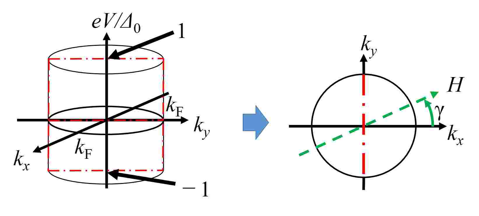
Figure 8: Dash dotted line (red line) represents a rectangular located at $k_{y}/k_{\mathrm{F}}=[-1,1]$ and $eV/\Delta_{0}=[-1,1]$ on $k_{y}-eV$ plane which are used for (b), (e) and (h) in Fig. 9, Fig. 11 and Fig. 13. Dashed line (green line) represents the direction of magnetic field which corresponds to the arrow in Fig. 1.

In this subsection, we discuss the magnetic field dependence of conductance. We consider the situation in which magnetic field is applied in the $x-y$ plane [Eq. (5)] and is rotated along the $z$ axis by $\gamma$ (Fig. 8). It is known that the applied magnetic field shifts the energy of quasiparticle as a Doppler effect Fogelström et al. (1997). In the usual case, ZBCP without magnetic field is split into two Fogelström et al. (1997); Tanuma et al. (2002b) or the height of ZBCP is suppressed Tanaka et al. (2002a, b) by the Doppler effect. For chiral $p$-wave superconductors, the height of ZBCP is controlled by the direction of the applied magnetic field Tanaka et al. (2002b). In contrast to this standard knowledge, we show a unique behavior whereby the Doppler effect can change the line shape of conductance from zero bias dip to zero bias peak, as shown in Fig. 9 ($\Delta_{\mathrm{3d}}^{\nu=1}$) and Fig. 11 ($\Delta_{\mathrm{3d}}^{\nu=2}$).

For $\alpha=\pi/8$ with $H=0$ [Fig. 9 (f), Fig. 11 (f)], $\sigma$ near $eV=0$ has a concave shape, and it changes into ZBCP for $H/H_{0}=0.1$ with $\gamma=\pi$ [Fig. 9 (c), Fig. 11 (c)]. The Doppler effect shifts the energy dispersion of the SABS along the vector $(\cos\gamma,\sin\gamma,0)$, as shown in Fig. 8. The SABS that is slightly above or below zero energy for $H=0$ can contribute to zero bias conductance in the presence of the magnetic field. For $\nu=1$, in Fig. 9 (e), there is no ZESABS. However, in the presence of the magnetic field for $\gamma=\pi$, an SABS exists around zero energy near $(k_{x},k_{y})=(0,\pm k_{\mathrm{F}})$ [Fig. 9 (b)]. We can also see the circle near $k_{x}^{2}/\cos^{2}(\pi/8)+k_{y}^{2}=k_{\mathrm{F}}^{2}$ of ZESABS in Fig. 9 (a), which does not exist in Fig. 9 (d). On the other hand, in the case that the direction of the magnetic field is opposite, $i.e$., $\gamma=0$, SABS around zero energy remains absent. [Fig. 9 (g) and Fig. 9 (h)]. As seen from Fig. 9 (a), the angle-resolved conductance near $(k_{x},k_{y})=(\pm k_{\mathrm{F}},0)$ is enhanced. In Fig. 10 (a), we can see how the ZBCP develops with increasing magnetic field. We can see the generation of ZBCP even for small magnitudes of $H$ with $H/H_{0}=0.01$. The magnitude of zero bias conductance as a function of $H$ is shown in Fig. 10 (b) and it is approximately a linear function of $H$.

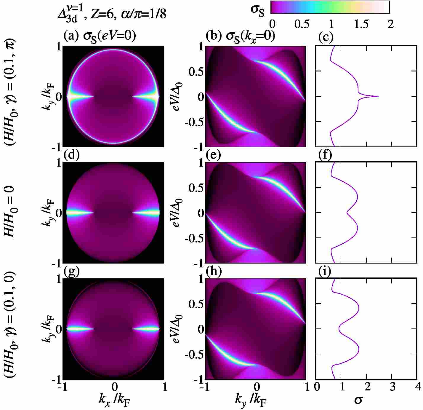
Figure 9: Angle-resolved conductance $\sigma_{\mathrm{S}}(eV,\mathbf{k}_{\parallel})$ for $\Delta_{\mathrm{3d}}^{\nu=1}$ with $\alpha=\pi/8$ are plotted as functions of ($k_{x},k_{y}$) with $eV=0$ [(a), (d), (g)] and ($k_{y},eV$) with $k_{x}=0$ [(b), (e), (h)] (see Fig. 8) and normalized conductance plotted as a function of $eV$ [(c), (f), (i)]. Normalized magnetic field $H/H_{0}$ is chosen to be 0.1 with $\gamma=\pi$ [(a), (b), (c)], 0 [(d), (e), (f)], 0.1 with $\gamma=0$ [(g), (h), (i)].

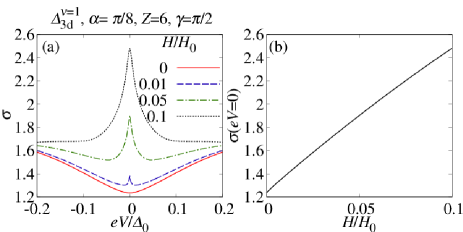
Figure 10: (a) Conductance is plotted as a function of $eV$ for $H/H_{0}=0$, 0.01, 0.05 and 0.1 with $\gamma=\pi/2$. (b) Conductance at $eV=0$ is plotted as a function of $H/H_{0}$. This plot is fitted by the linear function $f(H/H_{0})=aH/H_{0}+b$ with $(a,b)=(12.4,1.27)$.

A similar plot for $\nu=2$ with the same $\alpha$ is shown in Fig. 11. In this case, in contrast to Fig. 9, chiral edge mode crossing $k_{y}=0$ exists [see Fig. 7 (h-ii) and Fig. 11 (e)]. There are two kinds of branches of SABS: (1) chiral edge mode crossing $(k_{x},k_{y})=(0,0)$ and (2) SABS touching the ellipse given by $k_{x}^{2}/\cos^{2}(\pi/8)+k_{y}^{2}=k_{\mathrm{F}}^{2}$. The slope of the chiral edge mode becomes gradual (steep) for $\gamma=0$ ($\gamma=\pi$) in the presence of the magnetic field. The contribution to zero bias conductance becomes suppressed (enhanced) for $\gamma=\pi$ ($\gamma=0$). On the other hand, qualitative feature of SABS touching the ellipse is similar to that for $\nu=1$ shown in Fig. 9. In the presence of the magnetic field for $\gamma=\pi$, ZESABS exists near $(k_{x},k_{y})=(\pm k_{\mathrm{F}},0)$ and around the ellipse [Fig. 11 (a)]. Since the contribution to zero bias conductance from SABS touching the ellipse is dominant as compared to that of the chiral edge mode, the resulting $\sigma$ has a ZBCP. On the other hand, if the direction of the magnetic field is opposite, ZBCP is absent [Fig. 11 (i)]. In Fig. 12 (a), we show how ZBCP develops with increasing magnetic field. Even for small magnitude of $H$ ($H/H_{0}=0.01$), ZBCP appears similar to Fig. 10 (a). The magnitude of conductance at zero bias as a function of $H$ is shown in Fig. 12 (b) and it is an approximately linear function of $H$. The slope $a$ of the fitting function $f(H/H_{0})=aH/H_{0}+b$ is smaller than that for $\Delta_{\mathrm{3d}}^{\nu=1}$.

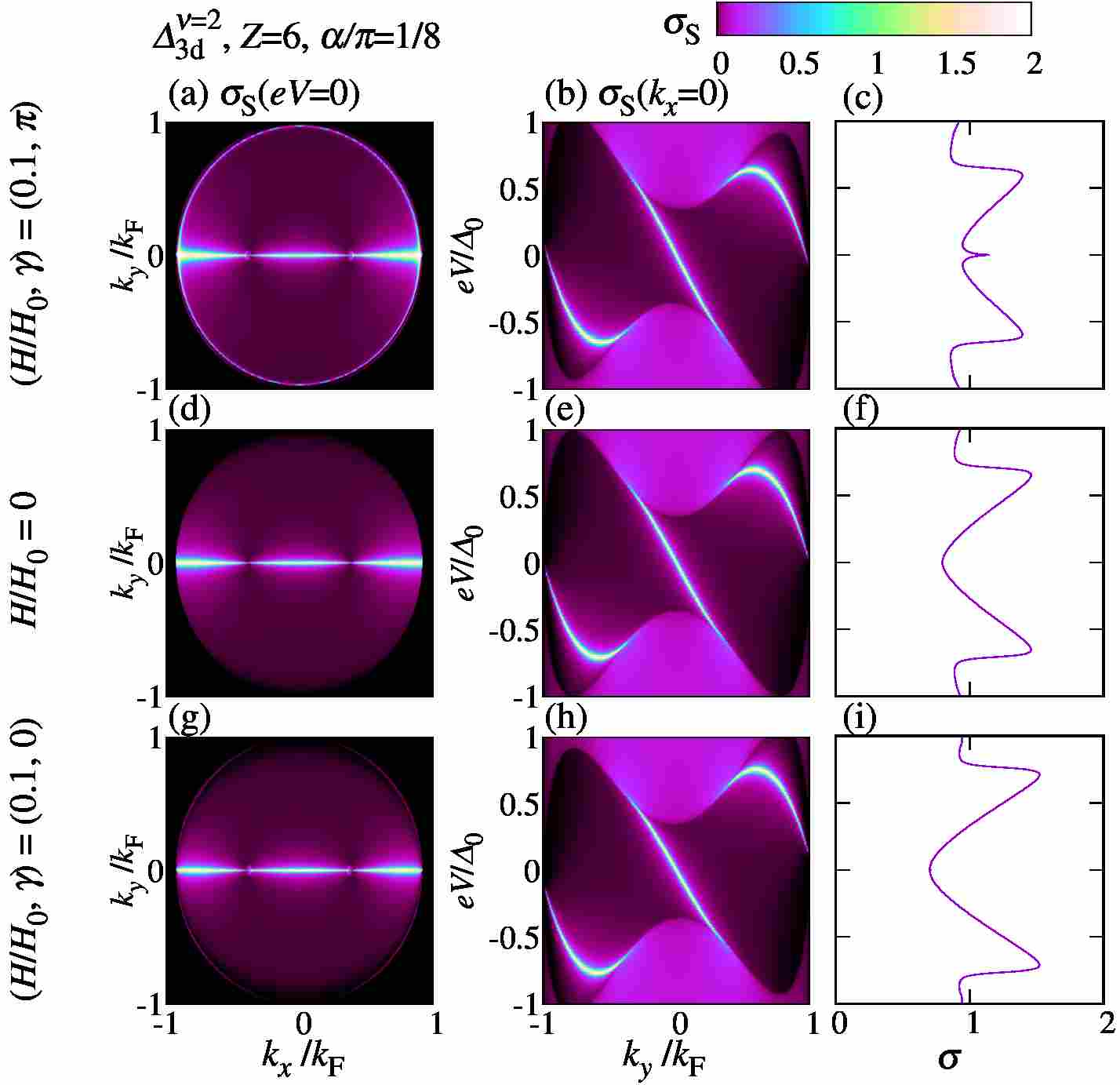
Figure 11: Angle-resolved conductance of $\Delta_{\mathrm{3d}}^{\nu=2}$ with $\alpha=\pi/8$. The model parameters used in this calculation is the same as in Fig. 9 except for pair potential $\Delta$.

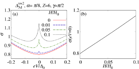
Figure 12: (a) Conductance is plotted as a function of $eV$ for $H/H_{0}=0$, 0.01, 0.05, and 0.1 with $\gamma=\pi/2$. (b) Conductance at $eV=0$ is plotted as a function of $H/H_{0}$. This plot is fitted by the linear function $f(H/H_{0})=aH/H_{0}+b$ with $(a,b)=(3.49,0.796)$.

Next, let us discuss special case of $\Delta_{\mathrm{3d}}^{\nu=1}$ for $\alpha=\pi/4$, at which there is no ZESABS without magnetic field [Fig. 7 (d-iii)]. The magnitude of the zero bias conductance for $H=0$ is very small [Fig. 13 (f)] and it becomes larger for $\gamma=\pi$ [Fig. 13 (c)] due to the similar mechanism explained in Fig. 9. For $\gamma=0$ [Fig. 13 (i)], although there is no SABS at zero-energy, the conductance becomes slightly larger than that for $H=0$.

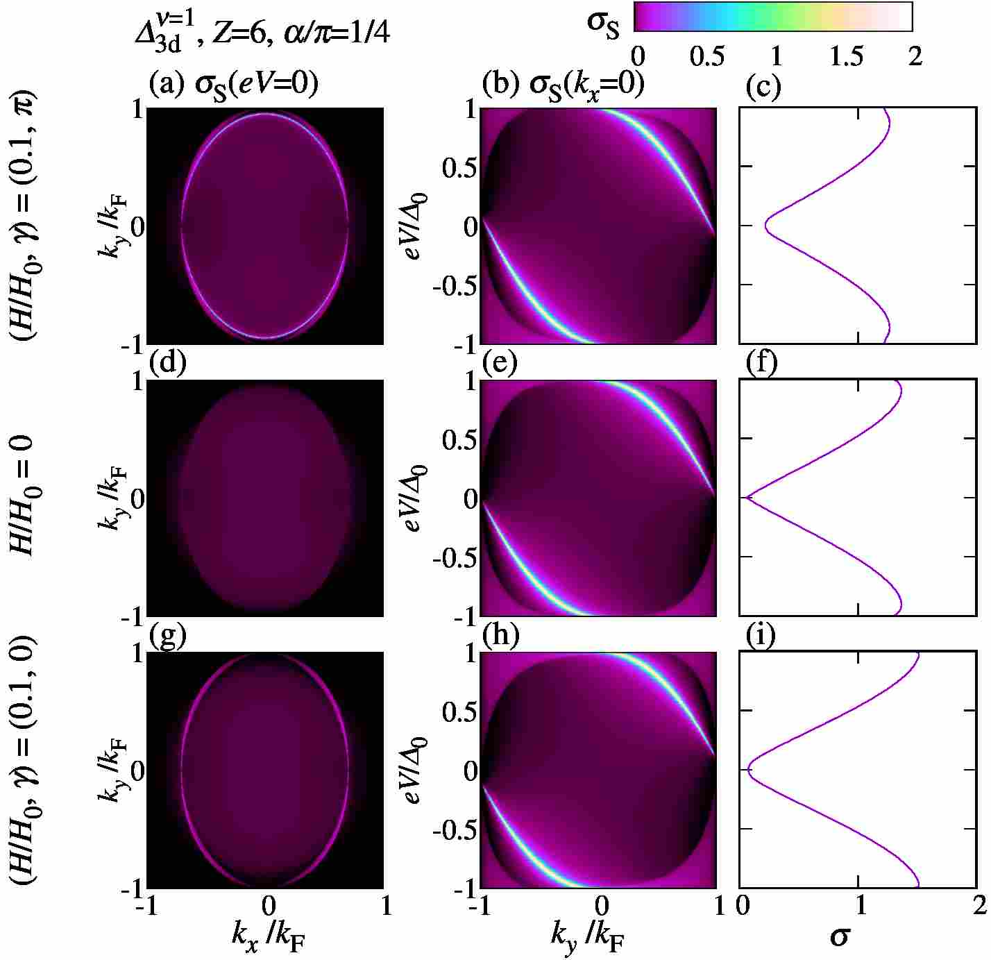
Figure 13: Angle-resolved conductance of $\Delta_{\mathrm{3d}}^{\nu=1}$ with $\alpha=\pi/4$. The parameters are the same as Fig. 9 except for $\alpha$.

Whether the magnitude of ZBCP becomes larger or smaller by applying an infinitesimally small magnitude of magnetic field is summarized in Table 4. For 2D-like chiral superconductors with $\nu=1$, since the energy dispersion of the SABS is given by $E(\mathbf{k}_{\parallel})=-k_{y}/k_{\mathrm{F}}$ [Eq. (31) and Eq. (32)], the magnitude of $\sigma(eV=0)$ becomes larger for $\gamma=0$ and smaller for $\gamma=\pi$. In other cases, there is no simple law owing to the complicated energy dispersion of the SABS. Using this table, we can classify five cases. If we make a junction for $\alpha=\pi/2$, we can distinguish between $\nu=0$ ($k^{\prime}_{z}$), $\nu=1$ [$k^{\prime}_{z}(k^{\prime}_{x}+ik^{\prime}_{y})$, $(k^{\prime}_{x}+ik^{\prime}_{y})$], and $\nu=2$ [$k^{\prime}_{z}(k^{\prime}_{x}+ik^{\prime}_{y})^{2}$, $(k^{\prime}_{x}+ik^{\prime}_{y})^{2}$]. Further, if we make a junction for $\alpha=0$, we can distinguish between $k^{\prime}_{z}(k^{\prime}_{x}+ik^{\prime}_{y})^{\nu}$ and $(k^{\prime}_{x}+ik^{\prime}_{y})^{\nu}$ with $(\nu=1,2)$.

Table 4: Line shape of $\sigma(eV)$ near $eV=0$ for $H=0$. p: peak, d: dip. Whether the magnitude of $\sigma(eV=0)$ is enhanced (suppressed) by magnetic field indicated by $\uparrow$ ($\downarrow$). We choose the infinitesimal applied magnetic field as $H/H_{0}=10^{-4}$. In the case $\Delta\propto k^{\prime}_{z}$, the value of $\sigma(eV=0)$ at $H>0$ with $\gamma=0$ and $\gamma=\pi$ are equivalent because $\sigma$ is a $\pi$ periodic function of $\gamma$.

			$\alpha$
$\Delta(\mathbf{k})$	$H/H_{0}$	$\gamma$	$0$	$\pi/8$	$\pi/4$	$3\pi/8$	$\pi/2$
$k^{\prime}_{z}$	0	-	p	p	p	p	d
	$10^{-4}$	$0,\pi$	$\downarrow$	$\downarrow$	$\downarrow$	$\downarrow$	$\uparrow$
$k^{\prime}_{z}(k^{\prime}_{x}+ik^{\prime}_{y})$	0	-	p	d	d	d	p
	$10^{-4}$	$0$	$\downarrow$	$\downarrow$	$\uparrow$	$\uparrow$	$\uparrow$
	$10^{-4}$	$\pi$	$\downarrow$	$\uparrow$	$\uparrow$	$\downarrow$	$\downarrow$
$(k^{\prime}_{x}+ik^{\prime}_{y})$	0	-	d	d	p	p	p
	$10^{-4}$	$0$	$\uparrow$	$\uparrow$	$\uparrow$	$\uparrow$	$\uparrow$
	$10^{-4}$	$\pi$	$\downarrow$	$\downarrow$	$\downarrow$	$\downarrow$	$\downarrow$
$k^{\prime}_{z}(k^{\prime}_{x}+ik^{\prime}_{y})^{2}$	0	-	p	d	d	p	d
	$10^{-4}$	$0$	$\downarrow$	$\downarrow$	$\uparrow$	$\uparrow$	$\downarrow$
	$10^{-4}$	$\pi$	$\downarrow$	$\uparrow$	$\downarrow$	$\downarrow$	$\uparrow$
$(k^{\prime}_{x}+ik^{\prime}_{y})^{2}$	0	-	d	p	p	d	d
	$10^{-4}$	$0$	$\uparrow$	$\uparrow$	$\uparrow$	$\downarrow$	$\downarrow$
	$10^{-4}$	$\pi$	$\uparrow$	$\downarrow$	$\downarrow$	$\uparrow$	$\uparrow$

To clarify $\gamma$ dependence of conductance, we plot $\sigma(eV=0)$ as a function of $\gamma$ for $\alpha=\pi/4$, and $\pi/2$ in Fig. 14. For $\alpha=0$, $\sigma(eV=0)$ is constant as a function of $\gamma$ owing to the rotational symmetry of the pair potentials (not shown). Since $\Delta_{\mathrm{3d}}^{\nu=0}$ conserves time reversal symmetry, $i.e$., the energy dispersion of the SABS has two-fold rotational symmetry [Fig. 6 (d-i)–(d-v)], $\sigma$ has $\pi$ periodicity [Fig. 14 (b), (c)]. In other cases, $\sigma(eV=0)$ has $2\pi$ periodicity due to time reversal symmetry breaking.

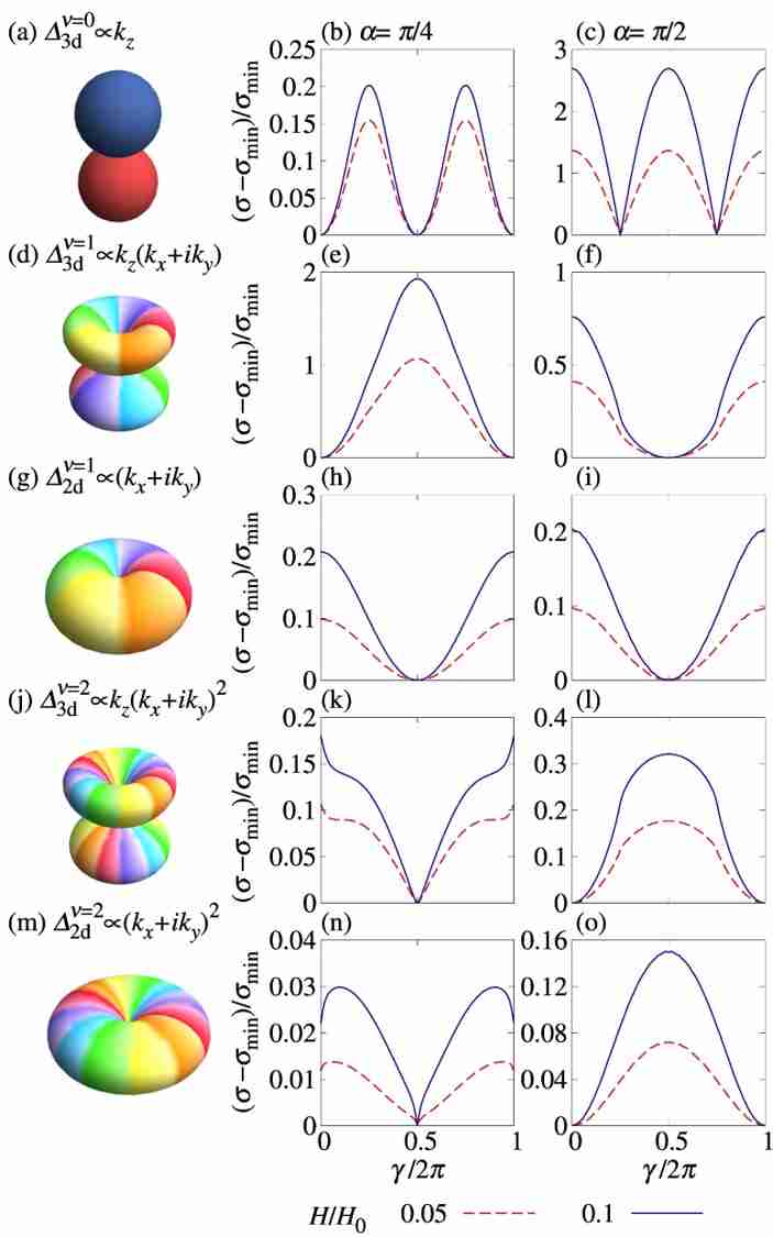
Figure 14: Normalized conductance at $eV=0$ is plotted as a function of $\gamma$ for $\nu=0,1,2$ with $Z=6$. Schematic pictures of the pair potential are shown in (a), (d), (g), (j), and (m). $\alpha=\pi/4$ for (b), (e), (h), (k), and (n). $\alpha=\pi/2$ for (c), (f), (i), (l), and (o). $\sigma_{\mathrm{min}}$ is a minimum value of $\sigma(eV=0)$ as a function of $\gamma$ for $H/H_{0}=0.05$ and $H/H_{0}=0.1$.

$\gamma$, which makes $\sigma(eV=0)$ largest is summarized in Table 5. In the case of $\Delta_{\mathrm{3d}}^{\nu=0}$ with $\alpha=\pi/2$, $\sigma(eV=0)$ becomes the smallest when the direction of the magnetic field is parallel to the direction of the projected line node. This result is consistent with that for the 2D $d$-wave case Vekhter et al. (1999); Tanuma et al. (2002b). However, in the case of 3D chiral superconductors with $\Delta_{\mathrm{3d}}^{\nu=1,2}$, this does not hold.

Table 5: $\gamma$ at which $\sigma(eV=0)$ becomes maximum as a function of $\gamma$ with $H/H_{0}=0.1$.

	$\alpha$
$\Delta$	$\pi/8$	$\pi/4$	$3\pi/8$	$\pi/2$
$k^{\prime}_{z}$	$\pi/2$,$3\pi/2$	$\pi/2$, $3\pi/2$	$\pi/2$, $3\pi/2$	$0$, $\pi$
$k^{\prime}_{z}(k^{\prime}_{x}+ik^{\prime}_{y})$	$\pi$	$\pi$	$0$	$0$
$(k^{\prime}_{x}+ik^{\prime}_{y})$	$\pi$	0	$\pi$	0
$k^{\prime}_{z}(k^{\prime}_{x}+ik^{\prime}_{y})^{2}$	$\pi$	$0$	$0$	$\pi$
$(k^{\prime}_{x}+ik^{\prime}_{y})^{2}$	$\sim 0$	$\sim 0$	$\pi$	$\pi$

III.3 Symmetry of pairing potential of UPt₃

Recently, the guide to determine the pairing symmetry of UPt₃ by using quasiparticle interference in a slab model was theoretically proposed Lambert et al. (2016). However, the role of the SABS in determining the charge transport in junctions has not yet been revealed. We also propose a way to determine the pairing symmetry by using Doppler shift. In this subsection, we consider $\Delta_{3\mathrm{d}}^{\nu=2}$, $\Delta_{E_{1u}}^{\mathrm{chiral}}$, and $\Delta_{E_{1u}}^{\mathrm{planar}}$ as candidates of the pairing symmetry. Crystal symmetry of UPt₃ is $P6_{3}/mmc$, so the pair potential around the $\Gamma$ point respects $D_{6h}$. In addition, various experiments Joynt and Taillefer (2002) indicate a spin-triplet paring and coexistence of point and line nodes. $\Delta_{3\mathrm{d}}^{\nu=2}$ and $\Delta_{E_{1u}}^{\rm planar}$ satisfy these properties and are possible candidates for the pairing symmetry of UPt₃ Mizushima et al. (2016). $\Delta_{E_{1u}}^{\mathrm{chiral}}$ does not have time reversal symmetry and $\Delta_{E_{1u}}^{\mathrm{planar}}$ has time reversal symmetry. For $\Delta_{E_{1u}}^{\mathrm{planar}}$, conductance is given by Eq. (27).

Firstly, let us discuss the SABS of $\Delta_{E_{1u}}^{\mathrm{chiral}}$ and $\Delta_{E_{1u}}^{\mathrm{planar}}$ (Fig. 15). The position of point and line nodes are shown on the Fermi surface for $\alpha=\pi/8$ [Fig. 15 (a-i)], $\alpha=\pi/4$ (a-ii), $\alpha=3\pi/8$ (a-iii), and $\alpha=\pi/2$ (a-iv). Corresponding projected point and line nodes on the $k_{x}-k_{y}$ plane are replotted from Fig. 15 (b-i) to (b-iv). In the case of $\Delta_{E_{1u}}^{\mathrm{planar}}$, as explained in Sec. II.2, the energy dispersion of the SABS for $\Delta_{E_{1u}}^{\mathrm{planar}}$ is $\pm E^{\mathrm{chiral}}(\mathbf{k})$. For example, Fig. 15 (e-i) is the same as (h-i) and Fig. 15 (h-i) and (i-i) are the energy dispersion of the SABS for $\Delta_{E_{1u}}^{\mathrm{planar}}$. Owing to the presence of two line nodes, there is no SABS at $\alpha=0$ for either $\Delta_{E_{1u}}^{\mathrm{chiral}}$ or $\Delta_{E_{1u}}^{\mathrm{planar}}$ (not shown). For $\alpha>0$, ZESABS of $\Delta_{E_{1u}}^{\mathrm{chiral}}$ [Fig. 15 (d-i)–(d-iv)] and that of $\Delta_{E_{1u}}^{\mathrm{planar}}$ [Fig. 15 (g-i)–(g-iv)] are the same because $S_{1}=S_{2}$ [Eq. (28) and Eq. (29)]. The number of ZESABSs is discussed in Appendix A.1.

The energy dispersion of the SABS becomes very complicated as seen from Fig. 15 (e-i) to (e-iv) for $\Delta_{E_{1u}}^{\mathrm{chiral}}$ and from [(h-i) and (i-i)] to [(h-iv) and (i-iv)] for $\Delta_{E_{1u}}^{\mathrm{planar}}$. This is due to the presence of two line nodes and two point nodes. The energy dispersion of the SABS at $\alpha=\pi/2$ is summarized in Table 6.

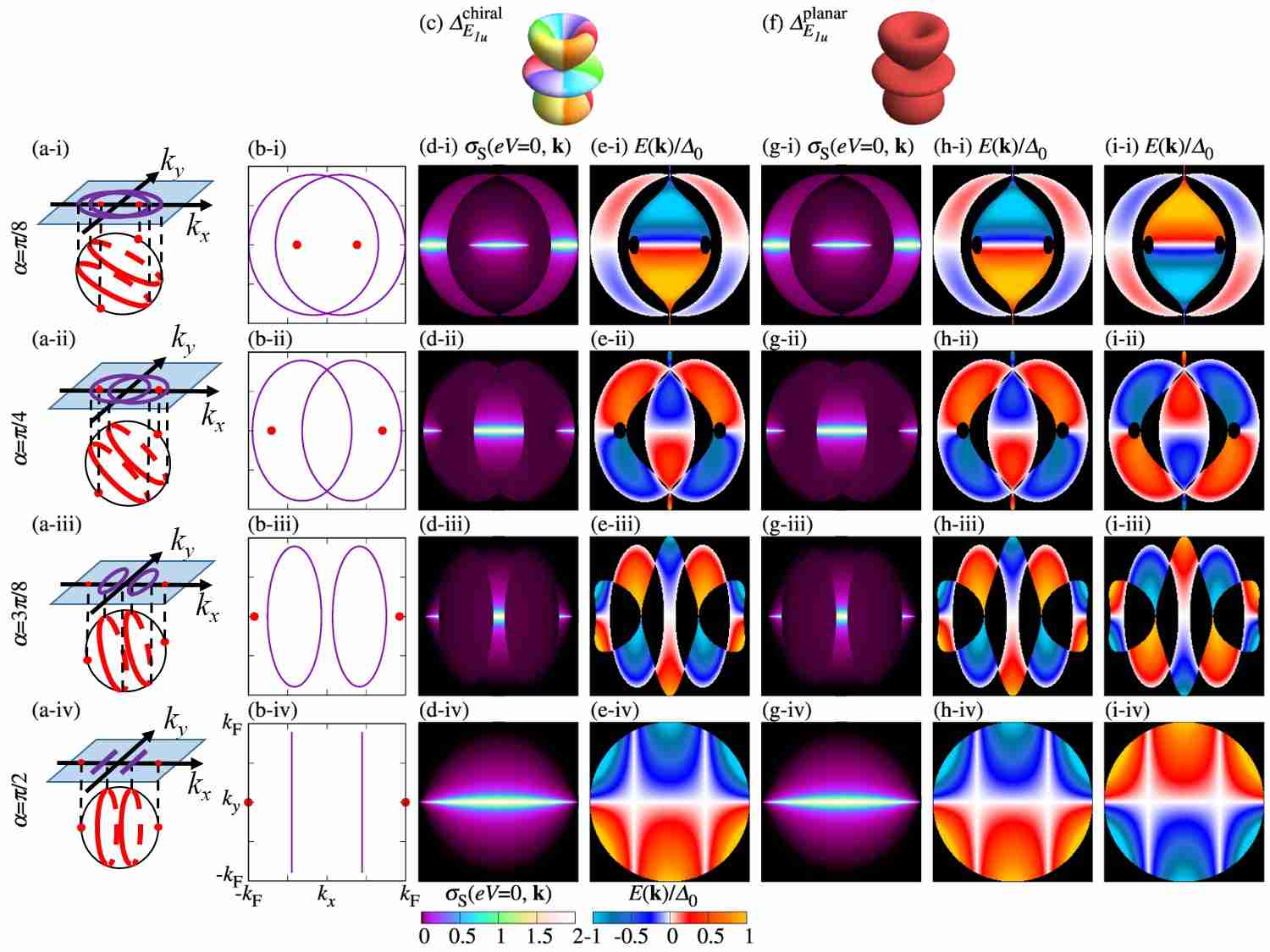
Figure 15: Schematic illustration of point nodes (red dots) and line nodes (red lines) for (a-i) $\alpha=\pi/8$, (a-ii) $\alpha=\pi/4$, (a-iii) $\alpha=3\pi/8$ and (a-iv) $\alpha=\pi/2$. Point nodes and line nodes projected on $k_{x}-k_{y}$ plane corresponding to (a-i)–(a-iv) are shown in (b-i)–(b-iv). Schematic picture of the pair potential for (c) $\Delta_{E_{1u}}^{\mathrm{chiral}}$ and (f) $\Delta_{E_{1u}}^{\mathrm{planar}}$. Angle-resolved zero bias conductance $\sigma_{\mathrm{S}}(eV=0,\mathbf{k}_{\parallel})$ with $Z=6$ is plotted as functions of $k_{x}$ and $k_{y}$ for $\Delta_{E_{1u}}^{\mathrm{chiral}}$ [(d-i)–(d-iv)] and for $\Delta_{E_{1u}}^{\mathrm{planar}}$ [(g-i)–(g-iv)]. The energy dispersion of SABS $E(\mathbf{k}_{\parallel})$ for given $\alpha$ are plotted as functions of $k_{x}$ and $k_{y}$ for $\Delta_{E_{1u}}^{\mathrm{chiral}}$ [(e-i)–(e-iv)] and for $\Delta_{E_{1u}}^{\mathrm{planar}}$ [(h-i) and (i-i)]–[(h-iv) and (i-iv)].

Table 6: The energy dispersion of SABS $E(\mathbf{k}_{\parallel})r_{E_{1u}}/\Delta_{0}$ at $\alpha=\pi/2$ is shown for $\Delta_{E_{1u}}^{\mathrm{chiral}}(\mathbf{k})$ and $\Delta_{E_{1u}}^{\mathrm{planar}}(\mathbf{k})$. $\hat{k}_{i}=k_{i}/k_{\mathrm{F}}(i=x,y,z)$.

$\Delta(\mathbf{k})$	$E(\mathbf{k}_{\parallel})r_{E_{1u}}/\Delta_{0}$
$\Delta_{E_{1u}}^{\mathrm{chiral}}(\mathbf{k})$	$-\hat{k}_{y}|5\hat{k}_{x}^{2}-1|$
$\Delta_{E_{1u}}^{\mathrm{planar}}(\mathbf{k})$	$\pm\hat{k}_{y}|5\hat{k}_{x}^{2}-1|$

The conductance for $\Delta_{3\mathrm{d}}^{\nu=2}$, $\Delta_{E_{1u}}^{\mathrm{chiral}}$, and $\Delta_{E_{1u}}^{\mathrm{planar}}$ is shown in Fig. 16. Although the angle-resolved conductance ($\sigma_{\mathrm{S}}$) of $\Delta_{E_{1u}}^{\mathrm{planar}}$ has a counter-propagating mode in addition to the same chiral edge mode shown in $\Delta_{E_{1u}}^{\mathrm{chiral}}$, the angular averaged conductance ($\sigma$) is the same [Fig. 16 (b)]. Therefore, we can distinguish $\Delta_{3\mathrm{d}}^{\nu=2}$ from ($\Delta_{E_{1u}}^{\mathrm{chiral}}$, $\Delta_{E_{1u}}^{\mathrm{planar}}$) by conductance but we cannot distinguish between $\Delta_{E_{1u}}^{\mathrm{chiral}}$ and $\Delta_{E_{1u}}^{\mathrm{planar}}$.

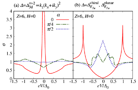
Figure 16: Normalized conductance for spin-triplet $f$-wave symmetry as a function of $eV$ for $\alpha=0$ (solid line), $\alpha=\pi/4$ (dash-dotted line), and $\alpha=\pi/2$ (dotted line). (a) $\Delta_{3\mathrm{d}}^{\nu=2}$ and (b) $\Delta_{E_{1u}}^{\mathrm{chiral}}$, $\sigma$ of $\Delta_{E_{1u}}^{\mathrm{planar}}$ coincides with that of $\Delta_{E_{1u}}^{\mathrm{chiral}}$.

To distinguish $\Delta_{E_{1u}}^{\mathrm{chiral}}$ from $\Delta_{E_{1u}}^{\mathrm{planar}}$, we discuss the directional dependence of the magnetic field on conductance (Fig. 17). Because $\Delta_{E_{1u}}^{\mathrm{chiral}}$ ($\Delta_{E_{1u}}^{\mathrm{planar}}$) does not have (has) time reversal symmetry, $\sigma(eV=0)$ has $2\pi$ ($\pi$) periodicity. The difference in conductance as a function of $eV$ with $H=0$ and that of $\gamma$ with the magnetic field between $\Delta_{\mathrm{3d}}^{\nu=2}$, $\Delta_{E_{1u}}^{\mathrm{chiral}}$ and $\Delta_{E_{1u}}^{\mathrm{planar}}$ are summarized in Table 7.

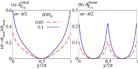
Figure 17: Normalized conductance at $Z=6$ as a function of $\gamma$ with $\alpha=\pi/2$. $H/H_{0}=0.1$ (solid line) and 0.05 (dashed line). (a) $\Delta_{E_{1u}}^{\mathrm{chiral}}$ and (b) $\Delta_{E_{1u}}^{\mathrm{planar}}$.

Table 7: Position of conductance peak with $(\alpha,H)=(0,0)$ (Fig. 16) and period of $\sigma(eV=0)$ as a function of $\gamma$ with $\alpha=\pi/2$ in the presence of the magnetic field [Fig. 14 (l) and Fig. 17].

	$\Delta_{\mathrm{3d}}^{\nu=2}$	$\Delta_{E_{1u}}^{\mathrm{chiral}}$	$\Delta_{E_{1u}}^{\mathrm{planar}}$
Conductance peak	$eV=0$	$eV=\Delta_{0}$	$eV=\Delta_{0}$
Period of $\sigma(\gamma)$	$2\pi$	$2\pi$	$\pi$

Whether ZBCP becomes larger or smaller when an infinitesimal magnitude of the magnetic field is applied is summarized in Table 8 and $\gamma$ which makes conductance largest is summarized in Table 9.

Table 8: Line shape of $\sigma(eV)$ near $eV=0$ with $H=0$. p: peak, d: dip. Whether the magnitude of $\sigma(eV=0)$ is enhanced (suppressed) by the magnetic field indicated by $\uparrow$ ($\downarrow$). We choose the infinitesimal magnitude of the magnetic field as $H/H_{0}=10^{-4}$. The value of $\sigma(eV)$ for $\Delta_{E_{1u}}^{\mathrm{planar}}$ at $\gamma=0$ and $\gamma=\pi$ are equivalent because $\sigma$ is a $\pi$ periodic function of $\gamma$.

			$\alpha$
$\Delta(\mathbf{k})$	$H/H_{0}$	$\gamma$	$0$	$\pi/8$	$\pi/4$	$3\pi/8$	$\pi/2$
$\Delta_{E_{1u}}^{\mathrm{chiral}}$	0	-	d	d	d	d	p
	$10^{-4}$	$0$	$\uparrow$	$\downarrow$	$\uparrow$	$\uparrow$	$\uparrow$
	$10^{-4}$	$\pi$	$\uparrow$	$\uparrow$	$\uparrow$	$\downarrow$	$\downarrow$
$\Delta_{E_{1u}}^{\mathrm{planar}}$	0	-	d	d	d	d	p
	$10^{-4}$	$0,\pi$	$\uparrow$	$\uparrow$	$\uparrow$	$\uparrow$	$\uparrow$

Table 9: The position of $\gamma$ at which $\sigma(eV=0)$ becomes maximum as a function of $\gamma$.

	$\alpha$
$\Delta$	$\pi/8$	$\pi/4$	$3\pi/8$	$\pi/2$
$\Delta_{E_{1u}}^{\mathrm{chiral}}$	$\pi$	0	0	0
$\Delta_{E_{1u}}^{\mathrm{planar}}$	0,$\pi$	0,$\pi$	0,$\pi$	0,$\pi$

Recently, Y. Yanase has proposed an extended version of $E_{2u}$ symmetryYanase (2016) as a model of the pairing symmetry of UPt₃. It is a linear combination of the spin-triplet $p$ and $f$-wave pairings. It is interesting to clarify whether the obtained results in Table 7 are changed by the disappearance of a line node by the mixing of a small magnitude of chiral $p$-wave pair potential and $\Delta_{3\mathrm{d}}^{\nu=2}$. We consider the non-unitary pair potential given by Eq. (25). For this purpose, we have used a general formula for tunneling conductance Eq. (26) derived in Appendix C. For $\eta=1$, the obtained conductance is shown in Fig. 18. In this case, there remain two point nodes and a line node [Fig. 3 (b-i)–(b-iii) and Fig. 4 (b-i)–(b-iii)]. When nonzero $\delta$ is introduced, ZBCP splits, but the shape of conductance is still distinct from that of $E_{1u}$ symmetry [Fig. 16 (b)]. For fixed $\delta$, the line shape of conductance $\sigma$ does not change qualitatively with the change of $\eta$ [Fig. 19 (a) and (b)]. Hence, it is expected that if the spin-triplet $p$-wave pair potential is additionally introduced into $\Delta_{3\mathrm{d}}^{\nu=2}$, $E_{1u}$ and the extended version of $E_{2u}$ can be distinguished by tunneling conductance.

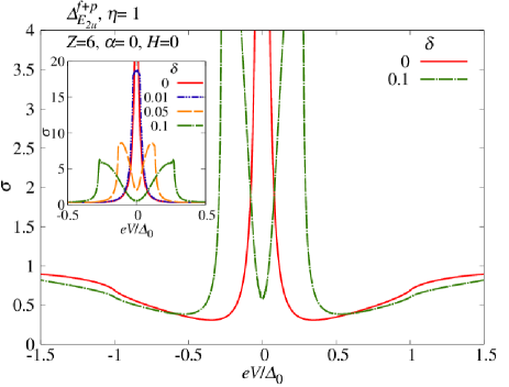
Figure 18: Normalized conductance $\sigma$ by its value in normal state for $\Delta_{E_{2u}}^{f+p}$ is plotted as a function of $eV$ for several $\delta$ with $\eta=1$ and $Z=6$. Inset is the magnification near $eV=0$.

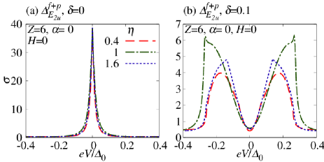
Figure 19: Normalized conductance $\sigma$ by its value in normal state for $\Delta_{E_{2u}}^{f+p}$ is plotted as a function of $eV$ for several $\eta$ with $Z=6$. (a) $\delta=0$ and (b) $\delta=0.1$.

IV Discussion and conclusion

In this paper, we have studied the surface Andreev bound state (SABS) and quasiparticle tunneling spectroscopy of three-dimensional (3D) chiral superconductors by changing the misorientation angle of superconductors. We have analytically derived a formula of the energy dispersion of SABS available for general pair potentials when an original $4\times 4$ matrix of BdG Hamiltonian can be decomposed into two blocks of $2\times 2$ matrices. We apply this formula to calculate the SABS for 3D chiral superconductors, where the pair potential is given by $\Delta_{0}k_{z}(k_{x}+ik_{y})^{\nu}/k_{\mathrm{F}}^{\nu+1}$ ($\nu=1,2$). The SABS has a complex momentum dependence, owing to the coexistence of point and line nodes. The number of branches of the energy dispersion of SABS with topological origin can be understood based on the winding and Chern numbers. We have calculated the tunneling conductance of normal metal / insulator / chiral superconductor junctions in the presence of the applied magnetic field, which induces a Doppler shift. In contrast to previous studies of Doppler effect on tunneling conductance, zero bias conductance dip can change into zero bias conductance peak by applying the magnetic field. This unique feature originates from the complicated energy dispersion of the SABS. We have also studied the SABS and tunneling conductance of UPt₃ focusing on four possible candidates of the pairing symmetry: $E_{2u}$, $E_{1u}$-planar, $E_{1u}$-chiral, and extended version of $E_{2u}$ pairings. Since the last pairing is non-unitary, we have developed a conductance formula, which is available for a general pair potential. By using this formula, we have shown that these four parings can be identified by tunneling spectroscopy both with and without magnetic field. Thus, our theory serves as a guide to determine the pairing symmetry of UPt₃.

In this paper, we are focusing on SABS and quasiparticle tunneling spectroscopy. As a next step, it will be interesting to calculate the Josephson effect in chiral superconductors, including spin-triplet non-unitary pairings Asano (2001), where both point and line nodes exist. Especially, it is known from the studies of $d$-wave superconductors, the role of $\alpha$ induces non-monotonic temperature dependence of maximum Josephson current Tanaka and Kashiwaya (1996); Barash et al. (1996a); Tanaka and Kashiwaya (1997); Barash et al. (1996b). The study of such a kind of exotic temperature dependence of the Josephson current will be really interesting.

In this paper, we have studied the case where a normal metal is ballistic. It is a challenging issue to extend our theory to diffusive normal metal (DN) / superconductor junctions where penetration of the Cooper pair owing to the proximity effect modifies the total resistance of the junctions Tanaka et al. (2003, 2004). In particular, it is known that the anomalous proximity effect with zero energy peak of the local density of states in DN via odd-frequency pairing occurs in spin-triplet superconductor junctions Tanaka and Kashiwaya (2004); Tanaka et al. (2005a); Asano et al. (2006); Tanaka et al. (2005b); Tanaka and Golubov (2007); Tanaka et al. (2007a, b). An extension of previous two-dimensional studies to three dimensions is also promising.

In the remainder, we discuss points related to the conductance formula [Eq. (26) or Eq. (65)].

(i) Doppler shift: Although the Doppler shift approximation is not quantitatively perfect, it is useful for the classification of pairing symmetry Tanuma et al. (2002a). When the penetration depth is much larger than the coherence length of superconductor, this approximation does work as far as we are discussing surface Andreev bound states and innergap tunneling conductance. This approximation has been actually done in the previous work in Eilenberger equation Tanaka et al. (2002b) and qualitatively reasonable results are obtained. Also, these results are qualitatively same as the results obtained by extended version of BTK theoryTanaka et al. (2002a).

(ii) Isotropic Fermi surface: In the point of view of the relation between topological invariant and surface Andreev bound state (SABS), the essential feature of SABS is determined by the node structure of pair potential in momentum space and symmetry of Hamiltonian when the magnitude of the pair potential is much smaller than Fermi energy. Thus, the qualitative nature of SABS is not so sensitive to the band structure. In the case that an actual Fermi surface is not topologically equivalent to the single isotropic Fermi surface, we must calculate SABS with the Fermi surface. For UPt₃, as far as superconducting pairing is formed on the Fermi surface nearest to $\Gamma$ point, it is expected that the qualitative shape of SABS in our paper can be compared to experimental results.

On the other hand, line shape of tunneling conductance is more or less influenced by band structures. When the obtained SABS has a flat band dispersion, the tunneling conductance has a zero bias conductance peak (ZBCP) shown by the previous studies of tight binding model Tanuma et al. (1998). On the other hand, when the SABS has a linear dispersion like chiral $p$-wave superconductor, the resulting line shape of tunneling conductance depends on band structures Yada et al. (2014).

As regards UPt₃, the energy band structures are complex. However, we think that one can design the experiment to greatly reduce such effect. For example, one can choose a kind of material belonging to UPt₃ family or with similar band structures as a normal side. As a result, the tunneling characteristic would depend mainly on the nodal structure of superconducting gap instead of the anisotropy of the continuous energy band. the superconducting gap structure will play a dominant role in the tunneling spectroscopy which this paper is focused on.

(iii) Applicability: If we focus on the low energy physics and a effective Hamiltonian of a material has a single Fermi surface, the conductance formula can be useful to discuss qualitative nature of superconductors. Especially to three dimensional superconductors which have complex nodes, for example, heavy Fermion compoundsSchnyder and Brydon (2015).

Appendix A Topological numbers

The 3D chiral superconductors host both a winding number and a Chern number relevant to ZESABSs. In a previous study, two of the present authors have discussed relevant topological numbers in 3D chiral superconductors with $\Delta_{\rm 3d}^{\nu=1}$ and $\Delta_{\rm 3d}^{\nu=2}$ by taking into account an additional symmetry Kobayashi et al. (2015). At this point, we explain topological numbers in 3D chiral superconductors with $\Delta^{\rm chiral}_{E_{1u}}$ and $\Delta_{\rm 3d}^{\nu>2}$.

A.1 Winding number in the case $\Delta^{\rm chiral}_{E_{1u}}$

Following the discussion in Ref. [Kobayashi et al., 2015], a winding number is defined in a similar way to the case $\Delta^{\nu=2}_{\rm 3d}$. However, $\Delta^{\rm chiral}_{E_{1u}}$ has two line nodes and is an even function of $k_{z}$, leading to a vanishing of zero-energy flat band for $\alpha=0$. Thus, in the following, we consider winding number for $\alpha\neq 0$ and $k_{y}=0$. In the $k_{x}-k_{z}$ plane, $\Delta^{\rm chiral}_{E_{1u}}$ is real, so we can define the winding number using time reversal symmetry and spin-rotation symmetry:

$$W(k_{x})\equiv\frac{-1}{4\pi i}\int^{\infty}_{-\infty}dk_{z}\text{Tr}[\Gamma H^{-1}(\mathbf{k})\partial_{k_{z}}H(\mathbf{k})]\Big{|}_{k_{y}=0},$$ (33)

where $H(\mathbf{k})$ is the BdG Hamiltonian with $\epsilon(\mathbf{k})=\frac{\hbar^{2}}{2m}(\mathbf{k}^{2}-k_{\mathrm{F}}^{2})$ and $\Delta^{\rm chiral}_{E_{1u}}$. The chiral operator, which anti-commutes with $H(\mathbf{k})$, is given by $\Gamma=-\sigma_{1}\tau_{2}$, where $\sigma_{\mu}$ and $\tau_{\mu}$ ($\mu=0,1,2,3$) are the identity matrix and the Pauli matrices in the spin and Nambu spaces, respectively. Furthermore, using the weak pairing assumption, Eq. (33) is reduced into

$$W(k_{x})=\sum_{\epsilon(\mathbf{k})=0}\text{sgn}[\partial_{k_{z}}\epsilon(\mathbf{k})]\cdot\text{sgn}[(5{k^{\prime}}_{z}^{2}-k_{\mathrm{F}}^{2}){k^{\prime}}_{x}],$$ (34)

where $k_{x}^{\prime}=k_{x}\cos\alpha-k_{z}\sin\alpha$ and $k_{z}^{\prime}=k_{x}\sin\alpha+k_{z}\cos\alpha$ and the summation is taken for $k_{z}$ satisfying $\epsilon(\mathbf{k})=0$.

To evaluate the winding number (34), we define the characteristic angles: $\alpha_{1}=\tan^{-1}\left(\frac{2}{\sqrt{5}+1}\right)$, $\alpha_{2}=\tan^{-1}\left(\frac{2}{\sqrt{5}-1}\right)$, and $\alpha_{3}=\tan^{-1}(2)$ and the positions of point and line nodes projected onto the $k_{x}$ line in the $(001)$ plane: $k^{\rm line}_{1}=\frac{k_{\mathrm{F}}}{\sqrt{5}}(\sin\alpha+2\cos\alpha)$ and $k^{\rm line}_{2}=\frac{k_{\mathrm{F}}}{\sqrt{5}}(-\sin\alpha+2\cos\alpha)$ for the line nodes and $k^{\rm point}=k_{\mathrm{F}}\sin\alpha$ for the point nodes (see Fig. 20). These angles satisfy $0<\frac{\pi}{8}<\alpha_{1}<\frac{\pi}{4}<\alpha_{2}<\alpha_{3}<\frac{3\pi}{8}<\frac{\pi}{2}$. Calculating Eq. (34), we obtain the winding number as follows:

• $0<\alpha\leq\alpha_{1}$
  

  $$W(k_{x})=\begin{cases}2&-k^{\rm line}_{1}<k_{x}<-k^{\rm line}_{2}\\ -2&-k^{\rm point}<k_{x}<k^{\rm point}\\ 2&k^{\rm line}_{2}<k_{x}<k^{\rm line}_{1}\\ 0&\text{otherwise}\end{cases}$$

• $\alpha_{1}<\alpha\leq\alpha_{2}$
  

  $$W(k_{x})=\begin{cases}2&-k^{\rm line}_{1}<k_{x}<-k^{\rm point}\\ -2&-k^{\rm line}_{2}<k_{x}<k^{\rm line}_{2}\\ 2&k^{\rm point}<k_{x}<k^{\rm line}_{1}\\ 0&\text{otherwise}\end{cases}$$

• $\alpha_{2}<\alpha\leq\alpha_{3}$
  

  $$W(k_{x})=\begin{cases}-2&-k^{\rm point}<k_{x}<-k^{\rm line}_{1}\\ -2&-k^{\rm line}_{2}<k_{x}<k^{\rm line}_{2}\\ -2&k^{\rm line}_{1}<k_{x}<k^{\rm point}\\ 0&\text{otherwise}\end{cases}$$

• $\alpha_{3}<\alpha\leq\frac{\pi}{2}$
  

  $$W(k_{x})=\begin{cases}-2&-k^{\rm point}<k_{x}<-k^{\rm line}_{1}\\ 2&k^{\rm line}_{2}<k_{x}<-k^{\rm line}_{2}\\ -2&k^{\rm line}_{1}<k_{x}<k^{\rm point}\\ 0&\text{otherwise}\end{cases}$$

The factor $2$ comes from the spin degrees of freedom. The obtained results are consistent with the ZESABSs in Fig. 15.

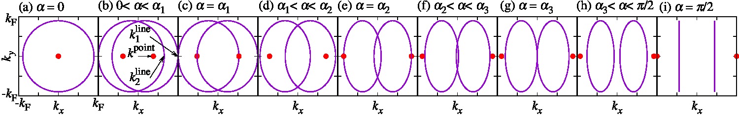
Figure 20: The position of point nodes and line nodes for $\Delta_{E_{1u}}^{\mathrm{chiral}}$ projected on the $k_{x}-k_{y}$ plane are shown for (a) $\alpha=0$, (b) $0<\alpha<\alpha_{1}$, (c) $\alpha=\alpha_{1}$, (d) $\alpha_{1}<\alpha<\alpha_{2}$, (e) $\alpha=\alpha_{2}$, (f) $\alpha_{2}<\alpha<\alpha_{3}$, (f) $\alpha=\alpha_{3}$, (h) $\alpha_{3}<\alpha<\pi/2$ and (i) $\alpha=\pi/2$. (b), (d), (h), and (i) are the same as Fig. 15 (b-i), (b-ii) (b-iii) and (b-iv), respectively. $k_{1}^{\mathrm{line}}$, $k_{2}^{\mathrm{line}}$ and $k^{\mathrm{point}}$ for $0<\alpha<\alpha_{1}$ are shown in (b).

A.2 Chern number in the case $\Delta_{\rm 3d}^{\nu>2}$

In 3D chiral superconductors with $\Delta_{\rm 3d}^{\nu=1}$ and $\Delta_{\rm 3d}^{\nu=2}$, ZESABSs are understood from both the winding number and the Chern number. On the other hand, 3D chiral superconductors with $\Delta_{\rm 3d}^{\nu>2}$ has the redundant ZESABSs for $0<\alpha\leq\frac{\pi}{4}$. To understand this type of ZESABSs, we introduce the Chern number defined on a cylinder:

$$N=\frac{i}{2\pi}\sum_{n\in\text{occ}}\int^{\infty}_{-\infty}dk_{z}\int_{0}^{2\pi}\rho d\theta\,\epsilon^{ab}\partial_{k_{a}}\langle u_{n}(\mathbf{k})|\partial_{k_{b}}|u_{n}(\mathbf{k})\rangle,$$ (35)

where the cylindrical coordinate is defined by $(\rho\cos\theta\pm k_{\mathrm{F}}\sin\alpha,\rho\sin\theta,k_{z})$, $|u_{n}(\mathbf{k})\rangle$ is an eigenstate of $H(\mathbf{k})$, and the summation is taken over all of occupied stats. We choose $\rho$ in such a way that the cylinder includes a single point node and does not touch the line node. Then, Eq. (35) gives $\pm 2\nu$ in analogy with the Chern number on the $k_{y}-k_{z}$ plane Kobayashi et al. (2015), where $2$ comes from the spin degrees of freedom. The nontrivial Chern number predicts $2\nu$ ZESABSs terminated at the point nodes. As shown in Fig. 7 (d-ii) and (g-ii), single and double ZESABSs terminated at the point nodes appear on the $k_{x}$ line, respectively. For $\nu>2$, we find $2\nu$ ZESABSs terminated at the point nodes [Fig. 21 (d) and (g)]. Note that the winding number also exists and explains ZESABSs in the $k_{x}$ line.

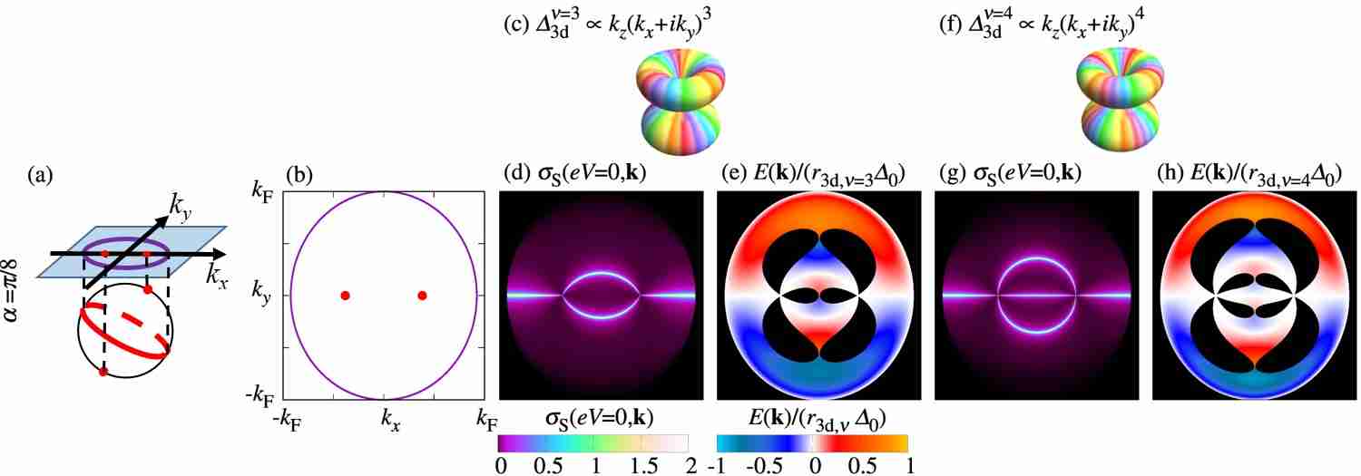
Figure 21: (a) Schematic illustration of point nodes (red dots) and a line node (red line) for $\alpha=\pi/8$. Point nodes and a line node projected on the $k_{x}-k_{y}$ plane corresponding to (a) are shown in (b). Schematic picture of pair potential for (c) $\Delta_{3\mathrm{d}}^{\nu=3}$ and (f) $\Delta_{3\mathrm{d}}^{\nu=4}$. (d) The angle-resolved zero bias conductance $\sigma_{\mathrm{S}}(eV=0,\mathbf{k}_{\parallel})$ at $Z=6$ are plotted as functions of $k_{x}$ and $k_{y}$ for (d) $\Delta_{3\mathrm{d}}^{\nu=3}$ and (g) $\Delta_{3\mathrm{d}}^{\nu=4}$. The energy dispersions of the SABS $E(\mathbf{k}_{\parallel})$ are plotted as functions of $k_{x}$ and $k_{y}$ for $\Delta_{3\mathrm{d}}^{\nu=3}$ (e) and for $\Delta_{3\mathrm{d}}^{\nu=4}$ (h).

Appendix B SABS

In Appendix B, we show how to derive the SABS. Since $|\Gamma_{\pm}|=1$ [$\Gamma_{\pm}$ is given by Eqs. (10) and (11)] is satisfied in in-gap state, we introduce $\theta_{\pm}$ as follows,

$$E =|\Delta_{+}|\cos\theta_{+},$$ (36)

$$=|\Delta_{-}|\cos\theta_{-}.$$ (37)

with $\Delta_{+}=\Delta(\mathbf{k})$, $\Delta_{-}=\Delta(\tilde{\mathbf{k}})$. Since $\theta_{+}$ and $\theta_{-}$ are not independent, we obtain

$$\kappa\frac{\cos\theta_{+}}{\cos\theta_{-}}=1,$$ (38)

with

$$\kappa=\frac{|\Delta_{+}|}{|\Delta_{-}|}.$$

$\theta_{+}$ ($\theta_{-}$) is used for the definition of $\Gamma_{+}$ ($\Gamma_{-}$) and is confined in the domain $0\leq\theta_{\pm}\leq\pi$. Then, $\Gamma_{\pm}$ is given by

$$\Gamma_{+} =\exp{[i(-\phi_{+}-\theta_{+})]},$$

$$\Gamma_{-} =\exp{[i(\phi_{-}-\theta_{-})]},$$

where $\phi_{\pm}$ is defined by $\Delta_{\pm}=|\Delta_{\pm}|\exp(i\phi_{\pm})$. Then, the SABS satisfies following conditions,

$$0=\mathrm{Im}\Gamma_{+}\Gamma_{-} =\sin\left(\phi-\theta_{+}-\theta_{-}\right),$$ (39)

$$1=\mathrm{Re}\Gamma_{+}\Gamma_{-} =\cos\left(\phi-\theta_{+}-\theta_{-}\right),$$ (40)

with

$$\phi=-\phi_{+}+\phi_{-}.$$

From Eqs. (39) and (40), the relation between $\phi$ and $\theta_{\pm}$ is obtained,

$$\phi-\theta_{+}-\theta_{-}= -2n\pi,$$

$$\Leftrightarrow\theta_{+}+\theta_{-}= 2n\pi+\phi,$$ (41)

where $n$ is an integer. The dispersion relation is given by Eq. (36) and Eq. (41) or Eq. (37) and Eq. (41).

In order to eliminate $\theta_{-}$, substitute Eq. (41) for Eq. (38). Then, we get

$$\cos\theta_{+}(\kappa-\cos\phi)=\sin\theta_{+}\sin\phi,$$

$$\Rightarrow \cos^{2}\theta_{+}\left[(\kappa-\cos\phi)^{2}+\sin^{2}\phi\right]=\sin^{2}\phi.$$ (42)

I)$\phi=2m\pi$ ($m$: integer) with $\kappa=1$

$(\theta_{+},\>\theta_{-})\neq(\pi/2,\>\pi/2)$ is satisfied by Eq. (41). From Eq. (38), we obtain

$$\cos\theta_{+}=\cos\theta_{-}.$$

This condition is held with $(\theta_{+},\theta_{-})=(0,\>0)$ or $(\pi,\>\pi)$. However, from Eq. (36) or Eq. (37), $E=\pm|\Delta_{+}|=\pm|\Delta_{-}|$ is satisfied. This means that the obtained energy dispersion is not inside the energy gap and is not the SABS (in-gap state).

II) $\phi\neq 2m\pi$ or $\kappa\neq 1$

From Eq. (42), we obtain $\cos\theta_{\pm}$ and $\sin\theta_{\pm}$ as follows

$$\cos\theta_{+} =\pm\frac{\sin\phi}{\sqrt{(\kappa-\cos\phi)^{2}+\sin^{2}\phi}},$$ (43)

$$\sin\theta_{+} =\frac{|\kappa-\cos\phi|}{\sqrt{(\kappa-\cos\phi)^{2}+\sin^{2}\phi}},$$ (44)

$$\cos\theta_{-} =\pm\frac{\sin\phi}{\sqrt{(\kappa^{-1}-\cos\phi)^{2}+\sin^{2}\phi}},$$ (45)

$$\sin\theta_{-} =\frac{|\kappa^{-1}-\cos\phi|}{\sqrt{(\kappa^{-1}-\cos\phi)^{2}+\sin^{2}\phi}},$$ (46)

where the sign of $\cos\theta_{+}$ and $\cos\theta_{-}$ are the same. We must check whether four equations from Eq. (43) to Eq. (46) are consistent with Eq. (41) or not. From Eq. (41), we obtain following relations,

$$\sin(\theta_{+}+\theta_{-})=\sin\phi,$$

$$\Leftrightarrow \pm\sin\phi\left(|\kappa-\cos\phi|+|\kappa^{-1}-\cos\phi|\right)$$

$$= \sin\phi\sqrt{(\kappa-\cos\phi)^{2}+\sin^{2}\phi}\sqrt{(\kappa^{-1}-\cos\phi)^{2}+\sin^{2}\phi},$$ (47)

$$\cos(\theta_{+}+\theta_{-})=\cos\phi,$$

$$\Leftrightarrow \sin^{2}\phi-|\kappa-\cos\phi||\kappa^{-1}-\cos\phi|$$

$$= \cos\phi\sqrt{(\kappa-\cos\phi)^{2}+\sin^{2}\phi}\sqrt{(\kappa^{-1}-\cos\phi)^{2}+\sin^{2}\phi}.$$ (48)

From Eq. (47), we must consider following four cases.

II-1) $\sin\phi=0$

i)$\phi=2l\pi$ ($l$: integer)

Substituting $\phi=2l\pi$ for Eq. (48); the left-hand side of Eq. (47) is negative but the right-hand side of it is positive. Therefore, there is no SABS.

ii)$\phi=(2l-1)\pi$ ($l$: integer)

$\phi=(2l-1)\pi$ satisfies Eq. (48). From Eq. (41), we obtain

$$\theta_{+}+\theta_{-}=\pi.$$

This equation contradicts the fact that the sign of $\cos\theta_{+}$ is equal to that of $\cos\theta_{-}$ except for $\theta_{\pm}=\pi/2$. Only for $\theta_{+}=\theta_{-}=\pi/2$, we obtain

$$\frac{\Delta_{+}}{|\Delta_{+}|}=-\frac{\Delta_{-}}{|\Delta_{-}|}.$$

This is the condition known for zero-energy SABS in unconventional superconductors Tanaka and Kashiwaya (1995); Kashiwaya and Tanaka (2000).

II-2) $\sin\phi\neq 0$

Hereafter, we suppose $\kappa\leq 1$. In the case of $\kappa>1$, the same discussion can be held with replacing $\kappa$ by $\kappa^{-1}$.

i)$\kappa-\cos\phi\geq 0$

In this case, Eq. (47) becomes

$$\pm(\kappa+\kappa^{-1}-2\cos\phi)= \sqrt{(\kappa-\cos\phi)^{2}+\sin^{2}\phi}\sqrt{(\kappa^{-1}-\cos\phi)^{2}+\sin^{2}\phi}.$$

The case of negative sign of the lefthand side does not satisfy above equation. If we choose positive sign, it is not difficult to confirm that the above equation is always satisfied.

On the other hand, Eq. (48) becomes

$$\sin^{2}\phi-1+\cos\phi(\kappa+\kappa^{-1})-\cos^{2}\phi= \cos\phi\left[(\kappa+\kappa^{-1})-2\cos\phi\right]$$

$$= \cos\phi\sqrt{(\kappa-\cos\phi)^{2}+\sin^{2}\phi}\sqrt{(\kappa^{-1}-\cos\phi)^{2}+\sin^{2}\phi}.$$ (49)

For $\cos\phi=0$, Eq. (49) is satisfied and and it means that it is a solution of the SABS. In the case of $\cos\phi\neq 0$, Eq. (48) becomes the same as Eq. (47) when we choose plus sign in Eq. (48). For $\kappa-\cos\phi\geq 0$, there always exists a solution of the SABS for arbitrary $\phi$.

ii)$\kappa-\cos\phi<0$

Eq. (47) becomes

$$\pm(-\kappa+\kappa^{-1}) =\sqrt{(\kappa-\cos\phi)^{2}+\sin^{2}\phi}\sqrt{(\kappa^{-1}-\cos\phi)^{2}+\sin^{2}\phi}.$$

The negative sign of the lefthand side does not satisfy this equation. By taking the square of this equation, we obtain

$$(\kappa-\kappa^{-1})^{2}= 2+(\kappa^{2}+\kappa^{-2})+4\cos^{2}\phi-4\cos\phi(\kappa+\kappa^{-1}),$$

$$\Leftrightarrow\cos\phi= \frac{1}{2}\left[\kappa+\kappa^{-1}\pm\sqrt{(\kappa-\kappa^{-1})^{2}}\right]$$

$$= \kappa,\>\kappa^{-1}.$$

The relation $\cos\phi=\kappa$ contradicts $\kappa-\cos\phi<0$ and $\cos\phi=\kappa^{-1}$ contradicts $\kappa^{-1}\geq 1$. Then, there is no solution of the SABS.

To summarize, if $\sin\phi=\sin(-\phi_{+}+\phi_{-})\neq 0$ is satisfied, the energy dispersion of the SABS is given by

$$E(\mathbf{k}_{\parallel})= \frac{|\Delta_{+}||\Delta_{-}|\sin\phi}{\sqrt{|\Delta_{+}|^{2}+|\Delta_{-}|^{2}-2|\Delta_{+}||\Delta_{-}|\cos\phi}}$$

$$= \frac{|\Delta_{+}||\Delta_{-}|\sin\phi}{|\Delta_{+}-\Delta_{-}|},$$

$$\mathrm{with}\>\> \left(\frac{|\Delta_{+}|}{|\Delta_{-}|}-\cos\phi\right)\left(\frac{|\Delta_{-}|}{|\Delta_{+}|}-\cos\phi\right)\geq 0.$$

For $\sin\phi=0$,

$$E(\mathbf{k}_{\parallel})= 0,$$

$$\mathrm{with}\>\frac{\Delta_{+}}{|\Delta_{+}|}= -\frac{\Delta_{-}}{|\Delta_{-}|}.$$

Appendix C Conductance for general pair potential

In this Appendx, we derive a conductance formula for any pair potential with single band superconductor where $\hat{\varepsilon}(\mathbf{k})$ in Eq. 1 does not have an off-diagonal element. In Sec. C.1, we introduce eigen vectors used for the wave function of superconducting side. In Sec. C.2, we solve boundary conditions and derive conductance. In Sec. C.3, we explain that conductance is invariant under the spin rotation.

C.1 Derivation of eigen vectors

In this subsection, we derive the eigen vectors of the BdG Hamiltonian. In Eq. (7), we define $\psi_{e,\sigma}^{\mathrm{S}}$ and $\psi_{h,\sigma}^{\mathrm{S}}$ as

$$\psi_{e,\uparrow}^{\mathrm{S}}= \begin{pmatrix}u_{+,p}\\ v_{+,p}\end{pmatrix},\>\psi_{e,\downarrow}^{\mathrm{S}}=\begin{pmatrix}u_{+,m}\\ v_{+,m}\end{pmatrix},$$

$$\psi_{h,\uparrow}^{\mathrm{S}}= \begin{pmatrix}v_{-,p}\\ u_{-,p}\end{pmatrix},\>\psi_{h,\downarrow}^{\mathrm{S}}=\begin{pmatrix}v_{-,m}\\ u_{-,m}\end{pmatrix}.$$

$u_{\pm,p(m)}$ and $v_{\pm,p(m)}$ satisfy

$$\begin{pmatrix}\tilde{\omega}_{+,p(m)}\sigma_{0}&\Delta_{+}\\ \Delta_{+}^{\dagger}&-\tilde{\omega}_{+,p(m)}\sigma_{0}\end{pmatrix}\begin{pmatrix}u_{+,p(m)}\\ v_{+,p(m)}\end{pmatrix} =E\begin{pmatrix}u_{+,p(m)}\\ v_{+,p(m)}\end{pmatrix},$$ (50)

$$\begin{pmatrix}-\tilde{\omega}_{-,p(m)}\sigma_{0}&\Delta_{-}\\ \Delta_{-}^{\dagger}&\tilde{\omega}_{-,p(m)}\sigma_{0}\end{pmatrix}\begin{pmatrix}v_{-,p(m)}\\ u_{-,p(m)}\end{pmatrix} =E\begin{pmatrix}v_{-,p(m)}\\ u_{-,p(m)}\end{pmatrix},$$ (51)

where $\sigma_{0}$ is the $2\times 2$ identity matrix and

$$\Delta_{\pm} =[D_{\pm}+\mathbf{d}_{\pm}\cdot\boldsymbol{\sigma}]i\sigma_{2}$$

$$\tilde{\omega}_{\pm,p} =\sqrt{E^{2}-(|\mathbf{d}_{\pm}|^{2}+|D_{\pm}|^{2}+|\mathbf{J_{\pm}}|)},$$ (52)

$$\tilde{\omega}_{\pm,m} =\sqrt{E^{2}-(|\mathbf{d}_{\pm}|^{2}+|D_{\pm}|^{2}-|\mathbf{J_{\pm}}|)},$$ (53)

$$\mathbf{J}_{\pm} =\pm\mathbf{F}_{\pm}+\mathbf{q}_{\pm}$$

$$\mathbf{F}_{\pm} =D_{\pm}\mathbf{d}_{\pm}^{*}+D_{\pm}^{*}\mathbf{d}_{\pm},$$

$$\mathbf{q}_{\pm} =i\mathbf{d}_{\pm}\times\mathbf{d}^{*}_{\pm},$$

with $D_{+}=D(\mathbf{k})$, $D_{-}=D(\tilde{\mathbf{k}})$, $\mathbf{d}_{+}=\mathbf{d}(\mathbf{k})$, $\mathbf{d}_{-}=\mathbf{d}(\tilde{\mathbf{k}})$ and $\tilde{\mathbf{k}}=(k_{x},k_{y},-k_{z})$. $\mathbf{F}_{\pm}$ and $\mathbf{q}_{\pm}$ are real-valued functions and perpendicular to each other. $D$ is a spin-singlet pair amplitude and $\mathbf{d}$ is a triplet one.

From Eqs. (50) and (51), we obtain following equations.

$$u_{+,p(m)}(E-\tilde{\omega}_{+,p(m)})(E+\tilde{\omega}_{+,p(m)})= \Delta_{+}\Delta_{+}^{\dagger}u_{+,p(m)},$$ (54)

$$u_{-,p(m)}(E-\tilde{\omega}_{-,p(m)})(E+\tilde{\omega}_{-,p(m)})= \Delta_{-}^{\dagger}\Delta_{-}u_{-,p(m)}.$$ (55)

To simplify above equations, we define $2\times 2$ matrices as

$$\check{\omega}_{\pm,pm}= \begin{pmatrix}\tilde{\omega}_{\pm,p}&0\\ 0&\tilde{\omega}_{\pm,m}\end{pmatrix},$$

$$u_{\pm}= \begin{pmatrix}u_{\pm,p}&u_{\pm,m}\end{pmatrix},$$

$$v_{\pm}= \begin{pmatrix}v_{\pm,p}&v_{\pm,m}\end{pmatrix}.$$

Eqs. (54) and (55) become

$$u_{+}(E\sigma_{0}-\check{\omega}_{+,pm})(E\sigma_{0}+\check{\omega}_{+,pm})= \Delta_{+}\Delta_{+}^{\dagger}u_{+},$$

$$u_{-}(E\sigma_{0}-\check{\omega}_{-,pm})(E\sigma_{0}+\check{\omega}_{-,pm})= \Delta_{-}^{\dagger}\Delta_{-}u_{-}.$$

$u_{+}$ and $u_{-}$ are given by Sigrist and Ueda (1991)

$$u_{+}= \tilde{a}_{+}\left(|\mathbf{J}_{+}|\sigma_{0}+\mathbf{J}_{+}\cdot\boldsymbol{\sigma}\right)(\sigma_{0}+\sigma_{3})+\tilde{b}_{+}\left(|\mathbf{J}_{+}|\sigma_{0}-\mathbf{J}_{+}\cdot\boldsymbol{\sigma}\right)(\sigma_{0}-\sigma_{3}),$$ (56)

$$u_{-}= \tilde{a}_{-}\left(|\mathbf{J}_{-}|\sigma_{0}+\mathbf{J}_{-}\cdot\boldsymbol{\sigma}^{*}\right)(\sigma_{0}+\sigma_{3})+\tilde{b}_{-}\left(|\mathbf{J}_{-}|\sigma_{0}-\mathbf{J}_{-}\cdot\boldsymbol{\sigma}^{*}\right)(\sigma_{0}-\sigma_{3}),$$ (57)

with

$$\tilde{a}_{\pm}(\tilde{b}_{\pm}) =\sqrt{\frac{1}{16|\mathbf{J_{\pm}}|[|\mathbf{J_{\pm}}|+(\mathbf{J_{\pm}})_{3}]}\frac{E+\tilde{\omega}_{\pm,p(m)}}{E}}.$$

By using $u_{\pm}$, $v_{\pm}$ can be expressed as

$$v_{+}= \Delta_{+}^{\dagger}u_{+}(E\sigma_{0}+\check{\omega}_{+,pm})^{-1},$$ (58)

$$v_{-}= \Delta_{-}u_{-}(E\sigma_{0}+\check{\omega}_{-,pm})^{-1}.$$ (59)

C.2 Conductance

Tunneling conductance for general pair potential is obtained by solving following boundary conditions [Eq. (13) and Eq. (14)].

$$e_{\sigma}+\begin{pmatrix}b_{\sigma}\\ a_{\sigma}\end{pmatrix}= \begin{pmatrix}u_{+}&v_{-}\\ v_{+}&u_{-}\end{pmatrix}\begin{pmatrix}c\\ d\end{pmatrix},$$ (60)

$$ik_{z}\begin{pmatrix}u_{+}&v_{-}\\ v_{+}&u_{-}\end{pmatrix}\begin{pmatrix}\sigma_{0}&0\\ 0&-\sigma_{0}\end{pmatrix}\begin{pmatrix}c\\ d\end{pmatrix}-ik_{z}e_{\sigma}+ik_{z}\begin{pmatrix}\sigma_{0}&0\\ 0&-\sigma_{0}\end{pmatrix}\begin{pmatrix}b_{\sigma}\\ a_{\sigma}\end{pmatrix}= \frac{2mU_{0}}{\hbar^{2}}\left[e_{\sigma}+\begin{pmatrix}b_{\sigma}\\ a_{\sigma}\end{pmatrix}\right],$$ (61)

with

$$e_{\uparrow}=(1,0,0,0)^{\mathrm{T}},\>\>e_{\downarrow}= (0,1,0,0)^{\mathrm{T}},\>\>a_{\sigma}=(a_{\sigma,\uparrow},a_{\sigma,\downarrow})^{\mathrm{T}},\>\>b_{\sigma}=(b_{\sigma,\uparrow},b_{\sigma,\downarrow})^{\mathrm{T}},\>\>c=(c_{\uparrow},c_{\downarrow})^{\mathrm{T}},\>\>d=(d_{\uparrow},d_{\downarrow})^{\mathrm{T}}.$$

We define

$$\hat{\Theta}_{\pm}= v_{\pm}(u_{\pm})^{-1},$$

$$Z^{\prime}= \frac{2mU_{0}}{k_{z}\hbar^{2}},$$

$$G= \begin{pmatrix}u_{+}&v_{-}\\ v_{+}&u_{-}\end{pmatrix}.$$

From Eqs. (58) and (59), $\hat{\Theta}_{+}$ and $\hat{\Theta}_{-}$ satisfy,

$$\hat{\Theta}_{+}= \Delta_{+}^{\dagger}u_{+}(E\sigma_{0}+\check{\omega}_{+,pm})^{-1}u_{+}^{-1},$$

$$\hat{\Theta}_{-}= \Delta_{-}u_{-}(E\sigma_{0}+\check{\omega}_{-,pm})^{-1}u_{-}^{-1}.$$

We can check that following $u_{\pm}^{-1}$ given by Eqs. (62) and (63) satisfy $u_{\pm}u_{\pm}^{-1}=\sigma_{0}$.

$$u_{+}^{-1}= \check{a}_{+}(\sigma_{0}+\sigma_{3})\left(|\mathbf{J}_{+}|\sigma_{0}+\mathbf{J}_{+}\cdot\boldsymbol{\sigma}\right)+\check{b}_{+}(\sigma_{0}-\sigma_{3})\left(|\mathbf{J}_{+}|\sigma_{0}-\mathbf{J}_{+}\cdot\boldsymbol{\sigma}\right)$$ (62)

$$u_{-}^{-1}= \check{a}_{-}(\sigma_{0}+\sigma_{3})\left(|\mathbf{J}_{-}|\sigma_{0}+\mathbf{J}_{-}\cdot\boldsymbol{\sigma}^{*}\right)+\check{b}_{-}(\sigma_{0}-\sigma_{3})\left(|\mathbf{J}_{-}|\sigma_{0}-\mathbf{J}_{-}\cdot\boldsymbol{\sigma}^{*}\right)$$ (63)

$$\check{a}_{\pm}= \sqrt{\frac{1}{4|\mathbf{J}_{\pm}|[|\mathbf{J}_{\pm}|+(\mathbf{J}_{\pm})_{3}]}\frac{E}{E+\tilde{\omega}_{\pm,p}}}$$

$$\check{b}_{\pm}= \sqrt{\frac{1}{4|\mathbf{J}_{\pm}|[|\mathbf{J}_{\pm}|+(\mathbf{J}_{\pm})_{3}]}\frac{E}{E+\tilde{\omega}_{\pm,m}}}$$

From Eqs. (62) and (63), $\hat{\Theta}_{+}$ and $\hat{\Theta}_{-}$ are obtained as

$$\hat{\Theta}_{+}= \frac{\Delta_{+}^{\dagger}}{2}\left[\left(\frac{1}{E+\tilde{\omega}_{+,p}}+\frac{1}{E+\tilde{\omega}_{+,m}}\right)+\left(\frac{1}{E+\tilde{\omega}_{+,p}}-\frac{1}{E+\tilde{\omega}_{+,m}}\right)\frac{\mathbf{J_{+}}}{|\mathbf{J_{+}}|}\cdot\boldsymbol{\sigma}\right],$$

$$\hat{\Theta}_{-}= \frac{\Delta_{-}}{2}\left[\left(\frac{1}{E+\tilde{\omega}_{-,p}}+\frac{1}{E+\tilde{\omega}_{-,m}}\right)+\left(\frac{1}{E+\tilde{\omega}_{-,p}}-\frac{1}{E+\tilde{\omega}_{-,m}}\right)\frac{\mathbf{J_{-}}}{|\mathbf{J_{-}}|}\cdot\boldsymbol{\sigma}^{*}\right].$$

If $\mathbf{F_{\pm}+q_{\pm}}=0$ is satisfied, from Eqs. (52), (53), (58), and (59), we obtain $\tilde{\omega}_{\pm,p}=\tilde{\omega}_{\pm,m}$ and

$$\hat{\Theta}_{+}= \frac{\Delta_{+}^{\dagger}}{E+\tilde{\omega}_{+,p}},$$

$$\hat{\Theta}_{-}= \frac{\Delta_{-}}{E+\tilde{\omega}_{-,p}}.$$

We obtain $a_{\sigma}$ and $b_{\sigma}$ from Eqs. (60) and (61).

$$\begin{pmatrix}b_{\sigma}\\ a_{\sigma}\end{pmatrix}= \left[I_{4}+G\begin{pmatrix}\sigma_{0}&0\\ 0&-\sigma_{0}\end{pmatrix}G^{-1}\begin{pmatrix}(1+iZ^{\prime})\sigma_{0}&0\\ 0&(-1+iZ^{\prime})\sigma_{0}\end{pmatrix}\right]^{-1}\left[-I_{4}+(1-iZ^{\prime})G\begin{pmatrix}\sigma_{0}&0\\ 0&-\sigma_{0}\end{pmatrix}G^{-1}\right]e_{\sigma},$$

where $I_{4}$ is the $4\times 4$ identity matrix. From the general relation of $2n$ $\times$ $2n$ matrix,

$$\begin{pmatrix}A&B\\ C&D\end{pmatrix}^{-1}$$

$$= \begin{pmatrix}\left(A-BD^{-1}C\right)^{-1}&\left(C-DB^{-1}A\right)^{-1}\\ \left(B-AC^{-1}D\right)^{-1}&\left(D-CA^{-1}B\right)^{-1}\end{pmatrix},$$ (64)

where $A$, $B$, $C$ and $D$ are $n\times n$ regular matrices, we obtain the following relation

$$G\begin{pmatrix}\sigma_{0}&0\\ 0&-\sigma_{0}\end{pmatrix}G^{-1}= \begin{pmatrix}\left(\sigma_{0}-\hat{\Theta}_{-}\hat{\Theta}_{+}\right)^{-1}\left(\sigma_{0}+\hat{\Theta}_{-}\hat{\Theta}_{+}\right)&-2\left(\sigma_{0}-\hat{\Theta}_{-}\hat{\Theta}_{+}\right)^{-1}\hat{\Theta}_{-}\\ 2\left(\sigma_{0}-\hat{\Theta}_{+}\hat{\Theta}_{-}\right)^{-1}\hat{\Theta}_{+}&-\left(\sigma_{0}-\hat{\Theta}_{+}\hat{\Theta}_{-}\right)^{-1}\left(\sigma_{0}+\hat{\Theta}_{+}\hat{\Theta}_{-}\right)\end{pmatrix}.$$

We define $2\times 2$ matrices $\alpha_{ij}$ as

$$\begin{pmatrix}\alpha_{11}&\alpha_{12}\\ \alpha_{21}&\alpha_{22}\end{pmatrix}=\left[I_{4}+G\begin{pmatrix}\sigma_{0}&0\\ 0&-\sigma_{0}\end{pmatrix}G^{-1}\begin{pmatrix}(1+iZ^{\prime})\sigma_{0}&0\\ 0&(-1+iZ^{\prime})\sigma_{0}\end{pmatrix}\right]^{-1}.$$

From Eq. (64), $\alpha_{ij}$ are obtained,

$$\alpha_{11}= (2-iZ^{\prime})\left[Z^{\prime 2}\hat{\Theta}_{-}\hat{\Theta}_{+}-(4+Z^{\prime 2})\sigma_{0}\right]^{-1}\left(\hat{\Theta}_{-}\hat{\Theta}_{+}-\sigma_{0}\right)^{-1}\left(\sigma_{0}+\frac{-iZ^{\prime}}{2-iZ^{\prime}}\hat{\Theta}_{-}\hat{\Theta}_{+}\right)\left(\sigma_{0}-\hat{\Theta}_{-}\hat{\Theta}_{+}\right),$$

$$\alpha_{22}= (2+iZ^{\prime})\left[Z^{\prime 2}\hat{\Theta}_{+}\hat{\Theta}_{-}-(4+Z^{\prime 2})\sigma_{0}\right]^{-1}\left(\hat{\Theta}_{+}\hat{\Theta}_{-}-\sigma_{0}\right)^{-1}\left(\sigma_{0}+\frac{iZ^{\prime}}{2+iZ^{\prime}}\hat{\Theta}_{+}\hat{\Theta}_{-}\right)\left(\sigma_{0}-\hat{\Theta}_{+}\hat{\Theta}_{-}\right),$$

$$\alpha_{12}= 2(-1+iZ^{\prime})\left[(4+Z^{\prime 2})\sigma_{0}-Z^{\prime 2}\hat{\Theta}_{-}\hat{\Theta}_{+}\right]^{-1}\left(\sigma_{0}-\hat{\Theta}_{-}\hat{\Theta}_{+}\right)^{-1}\hat{\Theta}_{-}\left(\sigma_{0}-\hat{\Theta}_{+}\hat{\Theta}_{-}\right),$$

$$\alpha_{21}= -2(1+iZ^{\prime})\left[(4+Z^{\prime 2})\sigma_{0}-Z^{\prime 2}\hat{\Theta}_{+}\hat{\Theta}_{-}\right]^{-1}\left(\sigma_{0}-\hat{\Theta}_{+}\hat{\Theta}_{-}\right)^{-1}\hat{\Theta}_{+}\left(\sigma_{0}-\hat{\Theta}_{-}\hat{\Theta}_{+}\right).$$

Finally, $b_{\sigma}$ and $a_{\sigma}$ are obtained

$$b_{\sigma}= \frac{-iZ^{\prime}}{2+iZ^{\prime}}\left(\sigma_{0}-\hat{\Theta}_{-}\hat{\Theta}_{+}\right)\left[\sigma_{0}-(1-\sigma_{\mathrm{N}})\hat{\Theta}_{-}\hat{\Theta}_{+}\right]^{-1}\tilde{e}_{\sigma},$$

$$a_{\sigma}= \sigma_{\mathrm{N}}\hat{\Theta}_{+}\left[\sigma_{0}-(1-\sigma_{\mathrm{N}})\hat{\Theta}_{-}\hat{\Theta}_{+}\right]^{-1}\tilde{e}_{\sigma},$$

where $\tilde{e}_{\sigma}$ is defined by $e_{\sigma}^{\mathrm{T}}=(\tilde{e}_{\sigma}^{\mathrm{T}},0,0)$. Then a general formula of tunneling conductance is expressed compactly by using $\hat{\Theta}_{+}$ and $\hat{\Theta}_{-}$.

$$\sigma_{\mathrm{S}}= \frac{1}{2}\sum_{\sigma}\left[1+a_{\sigma}^{\dagger}a_{\sigma}-b_{\sigma}^{\dagger}b_{\sigma}\right]$$

$$= \frac{\sigma_{\mathrm{N}}}{2}\mathrm{Tr}\left\{\left[\sigma_{0}-(1-\sigma_{\mathrm{N}})\hat{\Theta}_{+}^{\dagger}\hat{\Theta}_{-}^{\dagger}\right]^{-1}\left[\sigma_{0}+\sigma_{\mathrm{N}}\hat{\Theta}_{+}^{\dagger}\hat{\Theta}_{+}+(\sigma_{\mathrm{N}}-1)\hat{\Theta}_{+}^{\dagger}\hat{\Theta}_{-}^{\dagger}\hat{\Theta}_{-}\hat{\Theta}_{+}\right]\left[\sigma_{0}-(1-\sigma_{\mathrm{N}})\hat{\Theta}_{-}\hat{\Theta}_{+}\right]^{-1}\right\}.$$ (65)

C.3 Spin rotation

In this subsection, we explain that the conductance is invariant under the spin rotation. Under the spin rotation ($\Psi\rightarrow U\Psi$),

$$U= \begin{pmatrix}R&0\\ 0&R^{*}\\ \end{pmatrix},$$

$$R= e^{-i\boldsymbol{\theta}\cdot\boldsymbol{\sigma}/2},$$

pair potential $\Delta_{\pm}$ and $\mathbf{J}_{\pm}$ are transformed as

$$\Delta_{\pm}\rightarrow R\Delta_{\pm}R^{\mathrm{T}}$$

$$\mathbf{J}_{+}\cdot\boldsymbol{\sigma}\rightarrow R\mathbf{J}_{+}\cdot\boldsymbol{\sigma}R^{\dagger},$$

$$\mathbf{J}_{-}\cdot\boldsymbol{\sigma}^{*}\rightarrow R^{*}\mathbf{J}_{-}\cdot\boldsymbol{\sigma}^{*}R^{\mathrm{T}}.$$

$\hat{\Theta}_{\pm}$ is transformed as

$$\hat{\Theta}_{+}\rightarrow \frac{R^{*}\Delta_{+}^{\dagger}R^{\dagger}}{2}\left[\left(\frac{1}{E+\omega_{+,p}}+\frac{1}{E+\omega_{+,m}}\right)+\left(\frac{1}{E+\omega_{+,p}}-\frac{1}{E+\omega_{+,m}}\right)\frac{R\mathbf{J}_{+}\cdot\boldsymbol{\sigma}R^{\dagger}}{|\mathbf{J}_{+}|}\right]$$

$$=R^{*}\hat{\Theta}_{+}R^{\dagger},$$

$$\hat{\Theta}_{-}\rightarrow \frac{R\Delta_{-}R^{\mathrm{T}}}{2}\left[\left(\frac{1}{E+\omega_{-,p}}+\frac{1}{E+\omega_{-,m}}\right)+\left(\frac{1}{E+\omega_{-,p}}-\frac{1}{E+\omega_{-,m}}\right)\frac{R^{*}\mathbf{J}_{-}\cdot\boldsymbol{\sigma}^{*}R^{\mathrm{T}}}{|\mathbf{J}_{-}|}\right]$$

$$=R\hat{\Theta}_{-}R^{\mathrm{T}}.$$

Then the conductance is invariant under the spin rotation.

$$\sigma_{\mathrm{S}}\rightarrow \mathrm{Tr}\left[\sigma_{0}-(1-\sigma_{\mathrm{N}})R\hat{\Theta}_{+}^{\dagger}R^{\mathrm{T}}R^{*}\hat{\Theta}_{-}^{\dagger}R^{\dagger}\right]^{-1}\left[1+\sigma_{\mathrm{N}}R\hat{\Theta}_{+}^{\dagger}R^{\mathrm{T}}R^{*}\hat{\Theta}_{+}R^{\dagger}+(\sigma_{\mathrm{N}}-1)R\hat{\Theta}_{+}^{\dagger}R^{\mathrm{T}}R^{*}\hat{\Theta}_{-}^{\dagger}R^{\dagger}R\hat{\Theta}_{-}R^{\mathrm{T}}R^{*}\hat{\Theta}_{+}R^{\dagger}\right]$$

$$\left[\sigma_{0}-(1-\sigma_{\mathrm{N}})R\hat{\Theta}_{-}R^{\mathrm{T}}R^{*}\hat{\Theta}_{+}R^{\dagger}\right]^{-1}$$

$$= \mathrm{Tr}R\left[\sigma_{0}-(1-\sigma_{\mathrm{N}})\hat{\Theta}_{+}^{\dagger}\hat{\Theta}_{-}^{\dagger}\right]^{-1}R^{\dagger}R\left[1+\sigma_{\mathrm{N}}\hat{\Theta}_{+}^{\dagger}\hat{\Theta}_{+}+(\sigma_{\mathrm{N}}-1)\hat{\Theta}_{+}^{\dagger}\hat{\Theta}_{-}^{\dagger}\hat{\Theta}_{-}\hat{\Theta}_{+}\right]R^{\dagger}R\left[\sigma_{0}-(1-\sigma_{\mathrm{N}})\hat{\Theta}_{-}\hat{\Theta}_{+}\right]^{-1}R^{\dagger}$$

$$= \sigma_{\mathrm{S}}.$$