The Geometry of Parallelism

Abstract

We introduce a Geometry of Interaction model for higher-order quantum computation, and prove its adequacy for a fully fledged quantum programming language in which entanglement, duplication, and recursion are all available. This model is an instance of a new framework which captures not only quantum but also classical and probabilistic computation. Its main feature is the ability to model commutative effects in a parallel setting. Our model comes with a multi-token machine, a proof net system, and a $\mathsf{PCF}$-style language. Being based on a multi-token machine equipped with a memory, it has a concrete nature which makes it well suited for building low-level operational descriptions of higher-order languages.

1 Introduction

In classical computation, information is deterministic, discrete and freely duplicable. Already from the early days de Leeuw et al. [1955], however, determinism has been relaxed by allowing state evolution to be probabilistic. The classical model has then been further challenged by quantum computation Nielsen and Chuang [2011], a computation paradigm which is based on the laws of quantum mechanics.

Probabilistic and quantum computation are both justified by the very efficient algorithms they give rise to: think about Miller-Rabin primality test Miller [1975]; Rabin [1980], Shor’s factorization Shor [1994] but also the more recent algorithms for quantum chemistry Whitfield et al. [2011] or for solving linear systems of equations Harrow et al. [2009]. Finding out a way to conveniently express those algorithms without any reference to the underlying hardware, is then of paramount importance.

This has stimulated research on programming languages for probabilistic Kozen [1981]; Plotkin [1982] and quantum computation (see Gay [2006] for a survey), and recently on higher-order functional languages Selinger and Valiron [2006]; Green et al. [2013]; Pagani et al. [2014]. The latter has been epitomized by variations and extensions of the $\lambda$-calculus. In order to allow compositional reasoning, it is important to give a denotational semantics to those languages; maybe surprisingly, a large body of works in this direction is closely connected to denotational and interactive models of Linear Logic Girard [1987], in the style of Game Semantics Abramsky et al. [2000]; Hyland and Ong [2000] and the Geometry of Interaction Girard [1989].

The case of quantum computation is emblematic. The first adequate denotational model for a quantum programming language à la $\mathsf{PCF}$, only two years old Pagani et al. [2014], marries a categorical construction for the exponentials of linear logic Lafont [1988]; Melliès [2009] to a suitable extension of the standard model of quantum computation: the category of completely positive maps Selinger [2004]. The development of an interactive semantics has proved to be highly nontrivial, with results which are impressive but not yet completely satisfactory. In particular, the underlying language either does not properly reflect entanglement Hasuo and Hoshino [2011]; Delbecque [2009]; Delbecque and Panangaden [2008], a key feature of quantum computation, or its expressive power is too weak, lacking recursion and duplication Dal Lago and Zorzi [2014]; Dal Lago et al. [2014]. The main reason for this difficulty lies in the inherent non-locality of entanglement Nielsen and Chuang [2011].

In this paper we show that Girard’s Geometry of Interaction (GoI) indeed offers the right tools to deal with a fully fledged quantum programming language in which duplication and full recursion are available, when we equip GoI with an external quantum memory, a standard technique for operational models of quantum $\lambda$-calculi Selinger and Valiron [2006].

We go further: the approach we develop is not specific to quantum computation, and our quantum model is introduced as an instance of a new framework which models choice effects in a parametric way, via a memory structure. The memory structure comes with three operations: (1) allocation of fresh addresses in the memory, (2) low-level actions on the memory, and (3) choice based on the value of the memory at a given address. The notion of memory structure is flexible, the only requirement being commutativity of the operations. In Sec. 3.3 we show that different kinds of choice effects can be systematically treated: classical, probabilistic and quantum memory are all instances of this general notion. Therefore, the memory makes the model suitable to interpret classical, probabilistic and quantum functional programs. In particular, in the case of quantum memory, a low-level action is an application of unitary gate to the memory, while the choice performs a quantum measure.

The GoI model we give has a very concrete nature, as it consists of a class of token machines Danos and Regnier [1999]; Mackie [1995]. Their distinctive feature is to be parallel and multi-token Dal Lago et al. [2014, 2015] rather than single-token as in classic token machines Danos and Regnier [1999]. Being multi-token means that different computational threads can interact with each other and synchronize (think of this as a multi-player game, where players are able to collaborate and exchange information). The presence of multiple tokens allows to appropriately reflect non-locality in a quantum setting, but also to generally deal with parallelism and choice effects in a satisfactory way. We discuss why this is the case when we concretely present the machine (Sec. 5).

Finally, to deal with the combination of parallelism, probabilistic side-effects and non-termination, we develop a general notion of PARS, probabilistic abstract rewrite system. The results we establish on PARS are the key ingredient in the Adequacy proofs, but are also of independent interest. The issues at sake are non-trivial and we discuss them in the dedicated Sec. 1.2.

Contributions.

We present a Geometry of Interaction (GoI) model for higher-order quantum computation, which is adequate for a quantum programming language in which entanglement, duplication, and recursion are all available. Our model comes with a multi-token machine, a proof net system, and a $\mathsf{PCF}$-style language. More specifically, this paper’s contributions can be summarized as follows:

• we equip GoI with the ability to capture choice effects using a parametric notion of memory structure (Sec. 3);

• we show that the notion of memory structure is able to capture classical, probabilistic and quantum effects (Sec. 3.3);

• we introduce a construction which is parametric on the memory, and produces a class of multi-token machines (Sec. 5), proof net systems (Sec. 4) and $\mathsf{PCF}$-style languages (Sec. 6). We prove that (regardless of the specific memory) the multi-token machine is an adequate model of nets reduction (Th. 28), and the nets an adequate model of $\mathsf{PCF}$ term rewriting (Th. 29);

• we develop a general notion of parallel abstract rewrite system, which allows us to deal with the combination of parallelism and probabilistic choice in an infinitary setting (Sec. 2).

Being based on a multi-token machine associated to a memory, our model has a concrete nature which makes it well suited to build low-level operational descriptions of higher-order programming languages. In the remainder of this section, we give an informal overview of various aspects of our framework, and motivate with some examples the significance of our contribution.

This report is an extended version of Dal Lago et al. [2017].

1.1 Geometry of Interaction and Quantum Computation

Geometry of Interaction is interesting as semantics for programming languages Mackie [1994, 1995]; Ghica et al. [2011] because it is a high-level semantics which at the same time is close to low-level implementation and has a clear operational flavor. Computation is interpreted as a flow of information circulating around a network, which essentially is a representation of the underlying program. Computational steps are broken into low-level actions of one or more tokens which are the agents carrying the information around. A long standing open question is whether fully fledged higher-order quantum computation can be modeled operationally via the Geometry of Interaction.

1.1.1 Quantum Computation

As comprehensive references can be found in the literature Nielsen and Chuang [2011], we only cover the very few concepts that will be needed in this paper. Quantum computation deals with quantum bits rather than bits. The state of a quantum system can be represented with a density matrix to account for its probabilistic nature. However for our purpose we shall use in this paper the usual, more operational, non-probabilistic representation. Single quantum bits (or qubits) will thus be represented by a ray in a two-dimensional complex Hilbert space, that is, an equivalence class of non-zero vectors up to (complex) scalar multiplication. Information is attached to a qubit by choosing an orthonormal basis $(|{0}\rangle,|{1}\rangle)$: a qubit is a superposition of two classical bits (modulo scalar multiplication). If the state of several bits is represented with the product of the states of single bits, the state of a multi-qubit system is represented with the tensor product of single-qubit states. In particular, the state of an $n$-qubit system is a superposition of the state of an $n$-bit system. We consider superpositions to be normalized.

Two kinds of operations can be performed on qubits. First, one can perform reversible, unitary gates: they are unitary maps in the corresponding Hilbert space. A more exotic operation is the measurement, which is the only way to retrieve a classical bit out of a quantum bit. This operation is probabilistic: the probabilities depend on the state of the system. Moreover, it modifies the state of the memory. Concretely, if the original memory state is $\alpha_{0}|{0}\rangle\otimes\phi_{0}+\alpha_{1}|{1}\rangle\otimes\phi_{1}$ (with $\phi_{0}$ and $\phi_{1}$ normalized), measuring the first qubit would answer $x$ with probability $|\alpha_{x}|^{2}$, and the memory is turned into $|{x}\rangle\otimes\phi_{x}$. Note how the measurement not only modifies the measured qubit, but also collapses the global state of the memory.

The effects of measurements are counterintuitive especially in entangled system: consider the 2-qubit system $\frac{\sqrt{2}}{2}(|{00}\rangle+|{11}\rangle)$. This system is entangled, meaning that it cannot be written as $\phi\otimes\psi$ with $1$-qubit states $\phi$ and $\psi$. One can get such a system from the state $|{00}\rangle$ by applying first an Hadamard gate $\mathsf{H}$ on the second qubit, sending $|{0}\rangle$ to $\frac{\sqrt{2}}{2}(|{0}\rangle+|{1}\rangle)$ and $|{1}\rangle$ to $\frac{\sqrt{2}}{2}(|{0}\rangle-|{1}\rangle)$, therefore getting the state $\frac{\sqrt{2}}{2}(|{00}\rangle+|{01}\rangle)$, and then a $\mathsf{CNOT}$ (controlled-not) gate, sending $|{xy}\rangle$ to $|{x\oplus{}y}\rangle\otimes|{y}\rangle$. Measuring the first qubit will collapse the entire system to $|{00}\rangle$ or $|{11}\rangle$, with equal probability $\frac{1}{2}$.

Remark 1.

Notwithstanding the global collapse induced by the measurement, the operations on physically disjoint quantum states are commutative. Let $A$ and $B$ be two quantum states. Let $U$ act on $A$ and $V$ act on $B$ (whether they are unitaries, measurements, or combinations thereof). Consider now $A\otimes B$: applying $U$ on $A$ then $V$ on $B$ is equivalent to first applying $V$ on $B$ and then $A$ on $U$. In other words, the order of actions on physically separated quantum systems is irrelevant. We use this property in Sec. 3.3.3.

1.1.2 Previous Attempts and Missing Features

A first proposal of Geometry of Interaction for quantum computation is Hasuo and Hoshino [2011]. Based on a purely categorical construction Abramsky et al. [2002], it features duplication but not general entanglement: entangled qubits cannot be separately acted upon. As the authors recognize, a limit of their approach is that their GoI is single-token, and they already suggest that using several tokens could be the solution.

Example 2.

As an example, if $S=\frac{\sqrt{2}}{2}(|{00}\rangle+|{11}\rangle)$, the term

$${\tt let~{}}x\otimes y=S{\tt~{}in~{}}(Ux)\otimes(Vy)$$ (1)

cannot be represented in Hasuo and Hoshino [2011], because it is not possible to send entangled qubits to separate parts of the program.

A more recent proposal Dal Lago et al. [2014], which introduces an operational semantics based on multi-tokens, can handle general entanglement. However, it does neither handle duplication nor recursion. More than that, the approach relies on termination to establish its results, which therefore do not extend to an infinitary setting: it is not enough to “simply add” duplication and fix points.

Example 3.

In Dal Lago et al. [2014] it is not possible to simulate the program that tosses a coin (by performing a measurement), returns a fresh qubit on head and repeats on tail. In mock-up $\mathsf{ML}$, this program becomes

$${{\tt letrec}\,{f}\,{x}={({{\tt if}\,{x}\,{\tt then}\,{{\tt new}}\,{\tt else}\,{f\,(\mathsf{H}\,{\tt new}}}))}\,{\tt in}\,{(f\,(\mathsf{H}\,{\tt new}))}}$$

where new creates a fresh qubit in state $|{0}\rangle$ and where the if test performs a measurement on the qubit $x$. Note how the measure of $\mathsf{H}\,{{\tt new}}$ amounts to tossing a fair coin: $\mathsf{H}\,{{\tt new}}$ produces $\frac{\sqrt{2}}{2}(|{0}\rangle{+}|{1}\rangle)$. Measuring gives $|{0}\rangle$ and $|{1}\rangle$ with probability $\frac{1}{2}$.

Example 3 will be our leading example all along the paper. Furthermore, we shall come back to both examples in Sec. 7.1.1.

1.2 Parallel Choices: Confluence and Termination

When dealing with both probabilistic choice and infinitary reduction, parallelism makes the study of confluence and convergence highly non-trivial. The issue of confluence arises as soon as choices and duplication are both available, and non-termination adds to the challenges. Indeed, it is easy to see how tossing a coin and duplicating the result does not yield the same probabilistic result as tossing twice the coin. To play with this, let us take for example the following term of the probabilistic $\lambda$-calculus Ehrhard et al. [2014]:  $M=(\lambda x.x\;\mathtt{xor}\;x)((\mathtt{tt}\oplus\mathtt{ff})\oplus\Omega)$ where $\mathtt{tt}$ and $\mathtt{ff}$ are boolean constants, $\Omega$ is a divergent term, $\oplus$ is the choice operator (here, tossing a fair coin), and $\mathtt{xor}$ is the boolean operator computing the exclusive or. Depending on which of the two redexes we fire first, $M$ will evaluate to either the distribution $\{\mathtt{ff}^{\frac{1}{2}}\}$ or to the distribution $\{\mathtt{tt}^{\frac{1}{8}},\mathtt{ff}^{\frac{1}{8}}\}$. In ordinary, deterministic $\mathsf{PCF}$, any program of boolean type may or may not terminate, depending on the reduction strategy, but its normal form, if it exists, is unique. This is not the case for our probabilistic term $M$: depending on the choice of the redex, it evaluates to two distributions which are simply not comparable.

In the case of probabilistic $\lambda$-calculi, the way-out to this is to fix a reduction strategy; the issue however is not only in the syntax, it appears—at a more fundamental level—also in the model. This is the case for Ehrhard et al. [2014], where the model itself does not support parallel probabilistic choice. Similarly, in the development of a Game Semantics or Geometry of Interaction model for probabilistic $\lambda$-calculi, the standard approach has been to use a polarized setting, so to impose a strict form of sequentiality Danos and Harmer [2002]; Hoshino et al. [2014]. If instead we choose to have parallelism in the model, confluence is not granted and even the definition of convergence is non-trivial.

In this paper we propose a probabilistic model that is infinitary and parallel but confluent; to achieve this, in Sec. 2 we develop some results which are general to any probabilistic abstract rewrite system, and which to our knowledge are novel. More specifically, we provide sufficient conditions for an infinitary probabilistic system to be confluent and to satisfy a property which is a probabilistic analogous of the familiar “weak normalization implies strong normalization”. We then show that the parametric models which we introduce (both the proof nets and the multi-token machine) satisfy this property; this is indeed what ultimately grants the adequacy results.

1.3 Overview of the Framework, and Its Advantages

A quantum program has on one hand features which are specific to quantum computing, and on the other hand standard constructs. This is indeed the case for many paradigmatic languages; analyzing the features separately is often very useful. Our framework clearly separates (both in the language and in its operational model) the constructs which are common to all programming languages (e.g. recursion) and the features which are specific to some of them (e.g. measurement or probabilistic choice). The former is captured by a fixed operational core, the latter is encapsulated within a memory structure. This approach has two distinctive advantages:

• Facilitate Comparison between Different Languages: clearly separating in the semantics the standard features from the “notions of computation” which is the specificity of the language, allows for an easier comparison between different languages.

• Simplify the Design of a Language with Its Operational Model: it is enough to focus on the memory structure which encapsulates the desired effects. Once such a memory structure is given, the construction provides an adequate Geometry of Interaction model for a $\mathsf{PCF}$-like language equipped with that memory.

Memory structures are defined in Sec. 3, while the operational core is based on Linear Logic: a linearly-typed $\mathsf{PCF}$-like language, Geometry of Interaction, and its syntactical counterpart, proof nets. Proof nets are a graph-based formal system that provides a powerful tool to analyze the execution of terms as a rewriting process which is mostly parallel, local, and asynchronous.

More in detail, our framework consists of:

• a notion of memory structure, whose operations are suitable to capture a range of choice effects;

• an operational core, which is articulated in the three base rewrite systems (a proof net system, a GoI multi-token machine, and a $\mathsf{PCF}$-style language);

• a construction which is parametric on the memory, and lifts each base rewrite system into a more expressive operational system. We respectively call these systems: program nets, MSIAM machines and $\mathsf{PCF}_{\mathsf{AM}}$ abstract machines.

Finally, the three forms of systems are all related by adequacy results. As long as the memory operations satisfy commutativity, the construction produces an adequate GoI model for the corresponding $\mathsf{PCF}$ language. More precisely, we prove— again parametrically on the memory—that the MSIAM is an adequate model of program net reduction (Th. 28), and program nets are expressive enough to adequately represent the behavior of the $\mathsf{PCF}$ language (Th. 29).

1.4 Related Work

The low-level layer of our framework can be seen as a generalization and a variation of systems which are in the literature. The nets and multi-token machine we use are a variation of Dal Lago et al. [2015], the linearly typed $\mathsf{PCF}$ language is the one in Pagani et al. [2014] (minus lists and coproducts). What we add in this paper are the right tools to deal with challenges like probabilistic parallel reduction and entanglement. Neither quantum nor probabilistic choice can be treated in Dal Lago et al. [2015], because of the issues we clarified in Sec. 1.2. The specificity of our proposal is really its ability to deal with choice together with parallelism.

We already discussed previous attempts to give a GoI model of quantum computation, and their limits, in Sec. 1.1.2 above. Let us quickly go through other models of quantum computation. Our parametric memory is presented equationally: equational presentations of quantum memory are common in the literature Staton [2015]; Coecke et al. [2012]. Other models of quantum memories are instead based on Hilbert spaces and completely positive maps, as in Pagani et al. [2014]; Selinger [2004]. In both of these approaches, the model captures with precision the structure and behavior of the memory. Instead, in our setting, we only consider the interaction between the memory and the underlying computation by a set of equations on the state of the memory at a given address, the allocation of fresh addresses, and the low-level actions.

Finally, taking a more general perspective, our proposal is by no means the first one to study effects in an interactive setting. Dynamic semantics such as GoI and Game Semantics are gaining interest and attention as semantics for programming languages because of their operational flavor. Ghica [2007]; Muroya et al. [2016]; Hoshino et al. [2014] all deal with effects in GoI. A common point to all these works is to be single-token. While our approach at the moment only deals with choice effects, we indeed deal with parallelism, a challenging feature which was still missing.

2 PARS: Probabilistic Abstract Reduction Systems

Parallelism allows critical pairs; as we observed in Sec. 1.2, firing different redexes will produce different distributions and can lead to possibly very different results. Our parallel model however enjoys a property similar to the diamond property of abstract rewrite systems. Such a property entails a number of important consequences for confluence and normalization, and these results in fact are general to any probabilistic abstract reduction system. In particular, we define what we mean by strong and weak normalization in a probabilistic setting, and we prove that a suitable adaptation of the diamond property guarantees confluence and a form of uniqueness of normal forms, not unlike what happens in the deterministic case. Th. 11 is the main result of the section.

In a probabilistic context, spelling out the diamond property requires some care. We will introduce a strongly controlled notion of reduction on distributions ($\mathrel{\rightrightarrows}$). The need for this control has the same roots as in the deterministic case: please recall that strong normalization follows from weak normalization by the diamond property ( $b\leftarrow a\rightarrow c\Rightarrow b=c\lor\exists d(b\rightarrow d\leftarrow c)$ ) but not from subcommutativity ( $b\leftarrow a\rightarrow c\Rightarrow\exists d(b\rightarrow^{=}d\leftarrow^{=}c$) ) which appears very similar, but “leaves space” for an infinite branch.

2.1 Distributions and PARS

We start by setting the basic definitions. Given a set $A$, we note $\mathit{DST}(A)$ for the set of probability distributions on $A$: any $\mu\in\mathit{DST}(A)$ is a function from $A$ to $[0,1]$ such that $\sum_{a\in A}\mu(a)\leq 1$. A distribution $\mu$ is proper if $\sum_{a\in A}\mu(a)=1$. The distribution assigning $0$ to each element of a set $A$ is indicated with $\mathbf{0}$. We indicate with $\mathit{SUPP}(\mu)$ the support of a distribution $\mu$, i.e. the subset of $A$ whose image under $\mu$ is not $0$. On $\mathit{DST}(A)$, we define the relation $\subseteq$ point-wise: $\mu\subseteq\rho$ if $\mu(a)\leq\rho(a)$ for each $a\in A$.

A probabilistic abstract reduction system (PARS) is a pair $\mathcal{A}=(A,\rightarrow)$ consisting of a set $A$ and a relation ${\rightarrow}\subseteq{A\times\mathit{DST}(A)}$ (rewrite relation, or reduction relation) such that for each $(a,\mu)\in{\rightarrow}$, $\mathit{SUPP}(\mu)$ is finite. We write $a\rightarrow\mu$ for $(a,\mu)\in{\rightarrow}$. An element $a\in A$ is terminal or in normal form (w.r.t. $\rightarrow$) if there is no $\mu$ with $a\rightarrow\mu$, which we write $a\not\rightarrow$.

We can partition any distribution $\mu$ into a distribution $\mu^{\circ}$ on terminal elements, and a distribution $\bar{\mu}$ on elements for which there exists a reduction, as follows:

$$\mu^{\circ}(a)=\left\{\begin{array}[]{ll}\mu(a)&\mbox{if $a\not\rightarrow$,}\\ 0&\mbox{otherwise;}\end{array}\right.\qquad\qquad\bar{\mu}(a)=\mu(a)-\mu^{\circ}(a).$$

The degree of termination of $\mu$, written $\mathcal{T}(\mu)$, is $\sum_{a\in A}\mu^{\circ}(a)$.

We write $\mathrel{\looparrowright}$ for the reflexive and transitive closure of $\rightarrow$, namely the smallest subset of $A\times\mathit{DST}(A)$ closed under the following rules:

$$a\mathrel{\looparrowright}\mu a\rightarrow\mu\qquad a\mathrel{\looparrowright}\{a^{1}\}\qquad a\mathrel{\looparrowright}\mu+p\cdot\rho\lx@proof@logical@and a\mathrel{\looparrowright}\mu+\{b^{p}\}b\mathrel{\looparrowright}\rho b\notin\mathit{SUPP}(\mu)$$

We read $a\mathrel{\looparrowright}\mu$ as “$a$ reaches $\mu$”.

The Relation $\boldsymbol{\mathrel{\rightrightarrows}}$. In order to extend to PARS classical results on termination for rewriting systems, we define the binary relation $\mathrel{\rightrightarrows}$, which lifts the notion of one step reduction to distributions: we require that all non-terminal elements are indeed reduced. The relation ${\mathrel{\rightrightarrows}}\subseteq\mathit{DST}(A)\times\mathit{DST}(A)$ is defined as

$$\mu\mathrel{\rightrightarrows}\mu^{\circ}+\sum_{a\in\mathit{SUPP}(\bar{\mu})}\mu(a)\cdot\rho_{a}\lx@proof@logical@and\mu=\mu^{\circ}+\bar{\mu}\{a\rightarrow\rho_{a}\}_{a\in\mathit{SUPP}(\bar{\mu})}\,.$$

Please note that in the derivation above, we require $a\rightarrow\rho_{a}$ for each $a\in\mathit{SUPP}(\bar{\mu})$. Observe also that $\mu^{\circ}\mathrel{\rightrightarrows}\mu^{\circ}$ since $\mathit{SUPP}(\bar{\mu^{\circ}})=\emptyset$.

We write $\mu\mathrel{\rightrightarrows}^{n}\rho$ if $\mu$ reduces to $\rho$ in $n\geq 0$ steps; we write $\mu\mathrel{\rightrightarrows}^{*}\rho$ if there is any finite sequence of reductions from $\mu$ to $\rho$.

With a slight abuse of notation, in the rest of the paper we sometime write $\{a\}$ for $\{a^{1}\}$, or simply $a$ when clear from the context. As an example, we write $a\mathrel{\rightrightarrows}\mu$ for $\{a^{1}\}\mathrel{\rightrightarrows}\mu$. Moreover, the distribution $\{a_{1}^{p_{1}},\ldots,a_{n}^{p_{n}}\}$ will be often indicated as $\sum p_{i}\cdot\{a_{i}\}$ thus facilitating algebraic manipulations.

2.2 Normalization and Confluence

In this subsection, we look at normalization and confluence in the probabilistic setting, which we introduced in Sec. 2.1. We need to distinguish between weak and strong normalization. The former refers to the possibility to reach normal forms following any reduction order, while the latter (also known as termination, see Bezem and Klop [2003]) refers to the necessity of reaching normal forms. In both cases, the concept is inherently quantitative.

Definition 4 (Weak and Strong Normalization).

Let $p\in[0,1]$ and let $\mu\in\mathit{DST}(A)$ Then:

• $\mu$ weakly $p$-normalizes (or weakly normalizes with probability at least $p$) if there exists $\rho$ such that $\mu\mathrel{\rightrightarrows}^{*}\rho$ and $\mathcal{T}(\rho)\geq p$.

• $\mu$ strongly $p$-normalizes (or strongly normalizes with probability at least $p$) if there exists $n$ such that $\mu\mathrel{\rightrightarrows}^{n}\rho$ implies $\mathcal{T}(\rho)\geq p$, for all $\rho$.

The relation $\rightarrow$ is said uniform if for each $p$, and each $\mu\in\mathit{DST}(A)$, weak $p$-normalization implies strong $p$-normalization.

Following  Bezem and Klop [2003], we will also use the term $p$-termination for strong $p$-normalization, and refer to weak $p$-normalization as simply $p$-normalization.

Even the mere notion of convergent computation must be made quantitative here:

Definition 5 (Convergence).

The distribution $\mu\in\mathit{DST}(A)$ converges with probability $p$, written $\mu\Downarrow_{p}$, if $p={\sup_{\mu\mathrel{\rightrightarrows}^{*}\rho}\mathcal{T}(\rho)}.$

Observe that for every $\mu$ there is a unique probability $p$ such that $\mu\Downarrow_{p}$. Please also observe how Definition 5 is taken over all $\rho$ such that $\mu\mathrel{\rightrightarrows}^{*}\rho$, thus being forced to take into account all possible reduction orders. If $\rightarrow$ is uniform, however, we can reach the limit along any reduction order:

Proposition 6.

Assume $\rightarrow$ is uniform. Then for every $\mu$ such that $\mu\Downarrow_{p}$ and for every sequence of distributions ${(\rho_{n})_{n}}$ such that $\mu=\rho_{0}$ and $\rho_{n}\mathrel{\rightrightarrows}\rho_{n+1}$ for every $n$, it holds that $p=\lim_{n\to\infty}\mathcal{T}(\rho_{n})$. ∎

Remark 7.

Observe that because of Prop. 6, ${\sup_{\mu\mathrel{\rightrightarrows}^{*}\xi}\mathcal{T}(\rho)}={\sup_{\mu\mathrel{\looparrowright}\rho}\mathcal{T}(\rho)}$.

A PARS is said to be confluent iff $\mathrel{\rightrightarrows}$ is a confluent relation in the usual sense:

Definition 8 (Confluence).

The PARS $(A,\rightarrow)$ is said to be confluent if whenever $\tau\mathrel{\rightrightarrows}^{*}\mu$ and $\tau\mathrel{\rightrightarrows}^{*}\xi$, there exists $\rho$ such that $\mu\mathrel{\rightrightarrows}^{*}\rho$ and $\xi\mathrel{\rightrightarrows}^{*}\rho$.

2.3 The Diamond Property in a Probabilistic Scenario

In this section we study a property which guarantees confluence and uniformity.

Definition 9 (Diamond Property for PARS).

A PARS $(A,\rightarrow)$ satisfies the diamond property if the following holds. Assume $\mu\mathrel{\rightrightarrows}\nu$ and $\mu\mathrel{\rightrightarrows}\xi$. Then  (1) $\nu^{\circ}=\xi^{\circ}$ and   (2) $\exists\rho$ with $\nu\mathrel{\rightrightarrows}\rho$ and $\xi\mathrel{\rightrightarrows}\rho$.

As an immediate consequence:

Corollary 10 (Confluence).

If $(A,\rightarrow)$ satisfies the diamond property, then $(A,\rightarrow)$ is confluent. ∎

Finally, then, the diamond property ensures that weak $p$-normalization implies strong $p$-normalization, precisely like for usual abstract rewrite systems:

Theorem 11 (Normalization and Uniqueness of Normal Forms).

Assume $(A,\rightarrow)$ satisfies the diamond property. Then:

• Uniqueness of normal forms. $\mu\mathrel{\rightrightarrows}^{k}\rho$ and $\mu\mathrel{\rightrightarrows}^{k}\tau$ for some $k\in\mathbb{N}$ implies $\rho^{\circ}=\tau^{\circ}$.

• Uniformity. If $\mu$ is weakly $p$-normalizing (for some $p\in[0,1]$), then $\mu$ strongly $p$-normalizes, i.e., $\rightarrow$ is uniform.

Proof.

First note that (2) follows from (1). In order to prove (1), we use an adaptation of the familiar “tiling” argument. It is not exactly the standard proof because reaching some normal forms in a distribution is not the end of a sequence of reductions. Assume $\mu=\rho_{0}\mathrel{\rightrightarrows}\rho_{1}\mathrel{\rightrightarrows}...\mathrel{\rightrightarrows}\rho_{k}$, and $\mu\mathrel{\rightrightarrows}\tau_{1}\mathrel{\rightrightarrows}...\mathrel{\rightrightarrows}\tau_{k}$. We prove $\rho_{k}^{\circ}=\tau_{k}^{\circ}$ by induction on $k$. If $k=1$, the claim is true by Definition 9 (1). If $k>1$ we tile (w.r.t. $\mathrel{\rightrightarrows}$), as depicted below:
we build the sequence $\sigma_{0}=\tau_{1}$ $\mathrel{\rightrightarrows}\sigma_{1}...\mathrel{\rightrightarrows}\sigma_{k-1}$ (see the Fig. on the side) where each $\sigma_{i+1}$ ($i\geq 0$) is obtained via Definition 9 (2), from $\rho_{i}\mathrel{\rightrightarrows}\rho_{i+1}$ and $\rho_{i}\mathrel{\rightrightarrows}\sigma_{i}$, by closing the diamond. By Definition 9 (1) $\rho_{k}^{\circ}=\sigma_{k-1}^{\circ}$. Now we observe that $\tau_{1}\mathrel{\rightrightarrows}^{k-1}\tau_{k}$ and $\tau_{1}\mathrel{\rightrightarrows}^{k-1}\sigma_{k-1}$. Therefore we have (by induction) $\sigma_{k-1}^{\circ}=\tau_{k}^{\circ}$, from which we conclude $\rho_{k}^{\circ}=\tau_{k}^{\circ}$.∎

3 Memory Structures

In this section we introduce the notion of memory structure. Commutativity of the memory operations is ensured by a set of equations. To deal with the notion of fresh addresses, and avoid unnecessary bureaucracy, it is convenient to rely on nominal sets. The basic definitions are recalled below (for details, see, e.g., Pitts [2013]).

3.1 Nominal Sets

If $G$ is a group, then a $G$-set $(M,\cdot)$ is a set $M$ equipped with an action of $G$ on $M$, i.e. a binary operation $(\cdot):G\times M\longrightarrow M$ which respects the group operation. Let $I$ be a countably infinite set; let $M$ be a set equipped with an action of the group $\rm Perm(I)$ of finitary permutations of $I$. A support for $m\in M$ is a subset $A\subseteq I$ such that for all $\sigma\in\rm Perm(I)$, $\forall i\in A,\sigma i=i$ implies $\sigma\cdot m=m$. A nominal set is a $\rm Perm(I)$-set all of whose elements have finite support. In this case, if $m\in M$, we write ${\rm supp}(m)$ for the smallest support of $m$. The complementary notion of support is freshness: $i\in I$ is fresh for $m\in M$ if $i\not\in{\rm supp}(m)$. We write $(i~{}j)$ for the transposition which swaps $i$ and $j$.

We will make use of the following characterization of support in terms of transpositions: $A\subseteq I$ supports $m\in M$ if and only if for every $i,j\in I-A$ it holds that $(i~{}j)\cdot m=m$. As a consequence, for all $i,j\in I$, if they are fresh for $m\in M$ then $(i~{}j)\cdot m=m$.

3.2 Memory Structures

A memory structure $\mathrm{Mem}=(\mathrm{Mem},I,\cdot,\mathcal{L})$ consists of an infinite, countable set $I$ whose elements $i,j,k,\dots$ we call addresses, a nominal set $(\mathrm{Mem},\cdot)$ each of whose elements we call memory states, or more shortly, memories, and a finite set $\mathcal{L}$ of operations.

We write $I^{*}$ for the set of all tuples made from elements of $I$. A tuple is denoted with $(i_{1},\ldots,i_{n})$, or with $\vec{i}$. To a memory structure are associated the following maps.

• ${\rm test}:I\times\mathrm{Mem}\to\mathit{DST}(Bool\times\mathrm{Mem})$   (Observe that the set $\mathrm{Mem}$ might be updated by the operation ${\rm test}$: for this reason, it also appears in the codomain – See Remark 15),

• ${\rm update}:I^{*}\times\mathcal{L}\times\mathrm{Mem}\rightharpoonup\mathrm{Mem}$ (partial map),

• ${\rm arity}:\mathcal{L}\to\mathbb{N}$,

and the following three properties.

(1) The maps ${\rm test}$ and ${\rm update}$ respect the group action:

• $\sigma\cdot({\rm test}(i,m))={\rm test}(\sigma(i),\sigma\cdot m)$,

• $\sigma\cdot({\rm update}(\vec{i},x,m))={\rm update}(\sigma(\vec{i}),x,\sigma\cdot m)$,

where the action of $\rm Perm(I)$ is extended in the natural way to distributions and pairing with booleans.

(2) The action of a given operation on the memory is only defined for the correct arity. More precisely, ${\rm update}((i_{1}\ldots i_{n}),x,m)$ is defined if and only if the $i_{k}$’s are pairwise disjoint and ${\rm arity}(x)=n$.

(3) Disjoint tests and updates commute: assume that $i\neq j$, that $j$ does not meet $\vec{k}$, and that $\vec{k}$ and $\vec{k^{\prime}}$ are disjoint. First, updates on $\vec{k}$ and $\vec{k}^{\prime}$ commute: ${\rm update}(\vec{k},x,{\rm update}(\vec{k}^{\prime},x^{\prime},m))={\rm update}(\vec{k}^{\prime},x^{\prime},{\rm update}(\vec{k},x,m))$. Then, tests on $i$ commute with tests on $j$ and tests of $j$ commute with updates on $\vec{k}$. We pictorially represent these equations in Fig. 1. The drawings are meant to be read from top to bottom and represent the successive memories along action. Probabilistic behavior is represented with two exiting arrows, annotated with their respective probability of occurrence, and the boolean resulting from the test operation. Intermediate memories are unnamed and represented with “$\cdot$”. We write the formal equations in Appendix A.

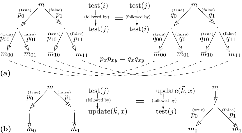
Figure 1: Commutation of Tests and Updates.

3.3 Instances of Memory Structures

The structure of memory is flexible and can accommodate several choice effects. Let us give some relevant examples. Typically, here $I$ is $\mathbb{N}$, but any countable set would do the job.

3.3.1 Deterministic, Integer Registers

The simplest instance of memory structure is the deterministic one, corresponding to the case of classical $\mathsf{PCF}$ (this subsumes, in particular, the case studied in Dal Lago et al. [2015]). Memories are simply functions $\mathbf{m}$ from $I$ to $\mathbb{N}$, of value 0 apart for a finite subset of $I$. The test on address $i$ is deterministic, and tests whether $\mathbf{m}(i)$ is zero or not. Operations in $\mathcal{L}$ may include the unary predecessor and successor, and for example the binary max operator.

Example 12.

A typical representation of this deterministic memory is a sequence of integers: indexes correspond to addresses and coefficients to values. A completely free memory is for example the sequence $\mathbf{m}_{0}=(0,0,0,\ldots)$. If $S$ corresponds to the successor and $P$ to the predecessor, here is what happens to the memory for some operations. The memory $\mathbf{m}_{1}:={\rm update}(0,S,\mathbf{m}_{0})$ is $(1,0,0,0,\ldots)$, the memory $\mathbf{m}_{2}:={\rm update}(1,S,\mathbf{m}_{1})$ is $(1,1,0,0,\ldots)$, and the memory $\mathbf{m}_{3}:={\rm update}(0,P,\mathbf{m}_{2})$ is $(0,1,0,0,\ldots)$. Finally, ${\rm test}(1,\mathbf{m}_{3})=({\rm false},(0,1,0,0,\ldots))$. Note that we do not need to keep track of an infinite sequence: a dynamic, finite list of values would be enough. We’ll come back to this in Sec. 3.3.3.

Remark 13.

The equations on memory structures enforce the fact that all fresh addresses (i.e., not on the support of the nominal set) have equal values. Note that however the conditions do not impose any particular “default” value. These equations also state that, in the deterministic case, a test action on $i$ can only modify the memory at address $i$. Otherwise, it could for example break the commutativity of update and test (unless $\mathcal{L}$ contains trivial operations, only).

3.3.2 Probabilistic, Boolean Registers

When the test operator is allowed to have a genuinely probabilistic behavior, the memory model supports the representation of probabilistic boolean registers. In this case, a memory $\mathbf{m}$ is a function from $I$ to the real interval $[0,1]$, whose values represent probabilities of observing “true”. The test on address $i$ could return

$$\mathbf{m}(i)\{({\rm true},\mathbf{m}\{i\mapsto 1\})\}+(1-\mathbf{m}(i))\{({\rm false},\mathbf{m}\{i\mapsto 0\})\}$$

Operations in $\mathcal{L}$ may for example include a unary “coin flipping” operation setting the value associated to $i$ to some fixed probability.

Example 14.

If as in Example 12 we represent the memory as a sequence, a memory filled with the value “false” would be $\mathbf{m}_{0}=(0,0,0,\ldots)$. Assume $c$ is the unary operation placing a fair coin at the corresponding address; if $\mathbf{m}_{1}$ is ${\rm update}(0,c,\mathbf{m}_{0})$, we have $\mathbf{m}_{1}=(\frac{1}{2},0,0,0,\ldots)$. Then ${\rm test}(0,\mathbf{m}_{1})$ is the distribution $\frac{1}{2}({\rm false},(0,0,0,0,\ldots))+\frac{1}{2}({\rm true},(1,0,0,0,\ldots))$.

3.3.3 Quantum Registers

A standard model for quantum computation is the QRAM model: quantum data is stored in a memory seen as a list of (quantum) registers, each one holding a qubit which can be acted upon. The model supports three main operations: creation of a new register, measurement of a register, and application of unitary gates on one or more registers, depending on the arity of the gate under scrutiny. This model has been used extensively in the context of quantum lambda-calculi Selinger and Valiron [2006]; Dal Lago and Zorzi [2014]; Pagani et al. [2014], with minor variations. The main choice to be made is whether measurement is destructive (i.e., if one uses garbage collection) or not (i.e., the register is not reclaimed).

A Canonical Presentation of Quantum Memory.

To fix things, we shall concentrate on the presentation given in Pagani et al. [2014]. We briefly recall it. Given $n$ qubits, a memory is a normalized vector in $(\mathbb{C}^{2})^{\otimes n}$ (equivalent to a ray). A linking function maps the position of each qubit in the list to some pointer name. The creation of a new qubit turns the memory $\phi\in(\mathbb{C}^{2})^{\otimes n}$ into $\phi\otimes|{0}\rangle\in(\mathbb{C}^{2})^{\otimes(n+1)}$. The measurement is destructive: if $\phi=\alpha_{0}{}q_{0}+\alpha_{1}{}q_{1}$, where each $q_{b}$ (with $b=0,1$) is normalized of the form $\sum_{i}\phi_{b,i}\otimes|{b}\rangle\otimes\psi_{b,i}$, then measuring $\phi$ returns $\sum_{i}\phi_{b,i}\otimes\psi_{b,i}$ with probability $|\alpha_{b}|^{2}$. Finally, the application of a $k$-ary unitary gate $U$ on $\phi\in(\mathbb{C}^{2})^{\otimes n}$ simply applies the unitary matrix corresponding to $U$ on the vector $\phi$. The language comes with a chosen set $\mathcal{U}$ of such gates.

Quantum Memory as a Nominal Set.

The quantum memory can be equivalently presented using a memory structure: in the following we shall refer to it as $\mathcal{Q}$. The idea is to use nominal set to make precise the hand-waved “pointer name”, and formalize the idea of having a finite core of ”in use” qubits, together with an infinite pool of fresh qubits. Let $\mathcal{F}_{0}$ be the set of (set-)maps from $I$ (the infinite, countable set of Sec. 3.2) to $\{0,1\}$ that have value $0$ everywhere except for a finite subset of $I$. We have a memory structure as follows.

$I$ is the domain of the set-maps in $\mathcal{F}_{0}$. The nominal set $(\mathrm{Mem},\cdot)$ is defined with $\mathrm{Mem}=\mathcal{H}_{0}$, i.e. the Hilbert space built from finite (complex) linear combinations over $\mathcal{F}_{0}$, while the group action $(\cdot)$ corresponds to permutation of addresses: $\sigma\cdot\mathbf{m}$ is simply the function-composition of $\sigma$ with the elements of $\mathcal{F}_{0}$ in superposition in $\mathbf{m}$. The support of a particular memory $\mathbf{m}$ is finite: it consists of the set of addresses that are not mapped to $0$ by some (set)-function in the superposition. The set of operations $\mathcal{L}$ is the chosen set $\mathcal{U}$ of unitary gates. The arity is the arity of the corresponding gate.

Finally, the update and test operations correspond respectively to the application of an unitary gate, and to a measurement followed by a (classical) boolean test on the result. We omit the formalization of these operations in the nominal set setting; instead we show how this presentation in terms of nominal sets is equivalent to the previous more canonical one.

Equivalence of the Two Presentations.

Let $\mathbf{m}\in\mathcal{Q}$. We can always consider a finite subset of $I$, say $I_{0}=\{i_{0}\ldots i_{n}\}$ for some integer $n$ such that all other addresses are fresh. As fresh values are $0$ in $\mathbf{m}$, then $\mathbf{m}$ is a superposition of sequences that are equal to 0 on $I\setminus I_{0}$. Then $\mathbf{m}$ can be represented as “$\phi\otimes|{000\ldots}\rangle$” for some (finite) vector $\phi$. We can omit the last $|{0000\ldots}\rangle$ and only work with the vector $\phi$: we are back to the canonical presentation of quantum memory. Update and test can then be defined on the nominal set presentation through this equivalence.

Equations.

Memory structures come with equations, which are indeed satisfied by quantum memories. Referring to Sec. 3.2 : (1) is simply renaming of qubits, (2) is a property of applying a unitary, and (3) holds because of the equations corresponding to the tensor of two unitaries or the tensor of a unitary and a measurement (see Remark 1).

Remark 15.

The quantum case makes clear why $\mathrm{Mem}$ appears in the codomain of test: in general the measurement of a register collapses the global state of the memory (see Sec. 1.1.1). The modified memory therefore has to be returned together with the result.

3.4 Overview of the Forthcoming Sections

We use memory structures to encapsulate effects in three different settings. In Sec. 4, we enrich proof nets with a memory, in Sec. 5, we enrich token machines with a memory, while in Sec. 6, we equip $\mathsf{PCF}$ terms with a memory. The construction is uniform for all the three systems, to which we refer as operational systems, as opposite to the base rewrite systems on top of which we build (see Sec. 1.3).

4 Program Nets and Their Dynamics

In this section, we introduce program nets. The base rewrite system on which they are built is a variation of SMEYLL nets, as introduced in Dal Lago et al. [2015]. SMEYLL nets are MELL (Multiplicative Exponential Linear Logic) proof nets extended with fixpoints (Y-boxes) which model recursion, additive boxes ($\bot$-boxes) which capture the if-then-else construct, and a family of sync nodes, introducing explicit synchronization points in the net.

The novelty of this section is the operational system which we introduce in Sec. 4.3, by means of our parametric construction: given a memory structure and SMEYLL nets, we define program nets and their reduction. We prove that program nets are a PARS which satisfies the diamond property, and therefore confluence and uniqueness of normal forms both hold. Program nets also satisfy cut elimination, i.e. deadlock-freeness of nets rewriting.

4.1 Formulas

The language of formulas is the same as for MELL. In this paper, we restrict our attention to the constant-only fragment, i.e.:

$$A\mathrel{::=}\mathsf{1}\mid\bot\mid A\otimes A\mid A\parr A\mid\,!A\mid\,?A.$$

The constants $1,\bot$ are the units. As usual, linear negation $(\cdot){}^{\bot}$ is extended into an involution on all formulas: $A{}^{\bot}{}^{\bot}\equiv A$, $1{}^{\bot}\equiv\bot$, $(A\otimes B){}^{\bot}\equiv A{}^{\bot}\parr B{}^{\bot}$, $(!A){}^{\bot}\equiv{}?A{}^{\bot}$. Linear implication is a defined connective: $A\multimap B\equiv A{}^{\bot}\parr B$. Positive formulas $P$ and negative formulas $N$ are respectively defined as: $P\mathrel{::=}\mathsf{1}\mid P\otimes P$, and $N\mathrel{::=}\bot\mid N\parr N$.

4.2 SMEYLL Nets

A SMEYLL net is a pre-net (i.e. a well-typed graph) which fulfills a correctness criterion.

Pre-Nets.

A pre-net is a labeled directed graph $R$ built over the alphabet of nodes represented in Fig. 2.

Edges. Every edge in $R$ is labeled with a formula; the label of an edge is called its type. We call those edges represented below (resp. above) a node symbol conclusions (resp. premises) of the node. We will often say that a node “has a conclusion (premise) $A$” as shortcut for “has a conclusion (premise) of type $A$”. When we need more precision, we explicitly distinguish an edge and its type and we use variables such as $e,f$ for the edges. Each edge is a conclusion of exactly one node and is a premise of at most one node. Edges which are not premises of any node are called the conclusions of the net.

Nodes. The sort of each node induces constraints on the number and the labels of its premises and conclusions. The constraints are graphically shown in Fig. 2. A sync node has $n\in\mathbb{N}$ premises of types $P_{1},P_{2},\cdots,P_{n}$ respectively and $n$ conclusions of the same types $P_{1},P_{2},\cdots,P_{n}$ as the premises, where each $P_{i}$ is a positive type. A sync node with $n$ premises and conclusions is drawn as $n$ many black squares connected by a line as in the figure. The total number of $\mathsf{1}$’s in the $P_{i}$’s is called the arity of the sync node.

We call boxes the nodes $\bot$, $!$, and $Y$. The leftmost conclusion of a box is said to be principal, while the other ones are auxiliary. The node $\bot$ has conclusion $\{\bot,\Gamma\}$ with $\Gamma\not=\emptyset$. The exponential boxes $!$ and $Y$ have conclusions $\{!A,?\Gamma\}$ ($\Gamma$ possibly empty). To each $!$-box (resp. $Y$-box) is associated a content, i.e. a pre-net of conclusions $\{A,?\Gamma\}$ (resp. $\{A,?A{}^{\bot},?\Gamma\}$). To each $\bot$-box are associated a left and a right content: each content is a pair $(\mathsf{bot},S)$, where $\mathsf{bot}$ is a new node that has no premise and one conclusion $\bot$, and $S$ is a pre-net of conclusions $\Gamma$. We represent a box $b$ and its content(s) as in Fig. 3. The nodes and edges in the content are said to be inside $b$. As is standard, we often call a crossing of the box border a door, which we treat as a node. We then speak of premises and conclusion of the principal (resp. auxiliary) door. Observe that in the case of $\bot$-box, the principal door has a left and a right premise.

Depth. A node occurs at depth 0 or on the surface in the pre-net $R$ if it is a node of $R$. It occurs at depth $n+1$ in $R$ if it occurs at depth $n$ in a pre-net associated to a box of $R$.

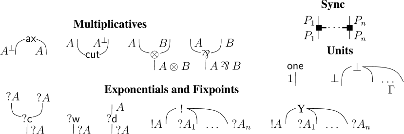
Figure 2: Nodes.

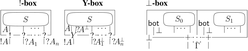
Figure 3: Boxes.

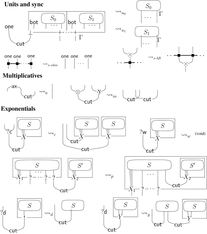
Figure 4: Nets Rewriting Rules.

Nets.

A net is given by a pre-net $R$ which satisfies the correctness criterion of Dal Lago et al. [2015], together with a total map ${\tt mkname}_{R}:{\tt SyncNode}(R)\to\mathcal{L}$, where $\mathcal{L}$ is a finite set of names and ${\tt SyncNode}(R)$ is the set of sync nodes appearing in $R$ (including those inside boxes); the map ${\tt mkname}_{R}$ is simply naming the sync nodes. From now on, we write $R$ for the triple $(R,\mathcal{L},{\tt mkname}_{R})$.

Correctness is defined by means of switching paths. A switching path in the pre-net $R$ is an undirected path on the graph $R$ (i.e. $R$ is regarded as an undirected graph) which uses at most one of the two premisses for each $\parr$ and $?c$ node, and at most one of conclusions for each sync node. A pre-net is correct if none of its switching paths is cyclic, and the content of each of its box is itself correct.

Reduction Rules.

Fig. 4 describes the rewriting rules on nets. Note that the redex in the top row has two possible reduction rules, $u_{0}$ and $u_{1}$. Note also the $y$ reduction, which captures the recursive behavior of the $Y$-box as a fixpoint (we illustrate this in the example below.) The metavariables $X,X_{1},X_{2}$ of Fig. 4 range over $\{!,Y\}$ and are used to uniformly specify reduction rules involving exponential boxes (i.e., $X$’s can be either $!$ or $Y$). The reduction of net has two constraints: (1.) surface reduction, i.e. a reduction step applies only when the redex is at depth 0, and (2.) exponential steps are closed, i.e. they only take place when the $!A$ premise of the cut is the principal conclusion of a box with no auxiliary conclusion. We come back on the former in Sec. 7.1.2.

As expected, the net reduction preserves correctness.

Example.

The “skeleton” of the program in Example 3 could be encoded as in the LHS of Fig. 5. The recursive function f is represented with a Y-box, and has type $!(1\multimap 1)={!}(\bot\parr 1)$. The test is encoded with a $\bot$-box: in one case we forget the function f by using $\mathsf{?w}$ and simply return a $\mathsf{one}$ node, and in the other case we apply a Hadamard gate, which is represented with a (unary) sync node. To the “in” part of the let-rec corresponds the dereliction node $\mathsf{?d}$, triggering reduction. With the rules presented in the previous paragraph, the net rewrites according to Fig. 5, where the Y-box has been unwound once. From there, we could reduce the $\mathsf{one}$ node with the sync node $\mathsf{H}$, but of course doing so we would not handle the quantum memory. In order to associate to reductions an action on the memory, we need a bit more, namely the notion of a program net which is introduced in Sec. 4.3.

Figure 5: Encoding of Example 3 and Net Rewrite.

4.3 Program Nets

Let ${\tt Inputs}(R)$ be the set of all occurrences of $\mathsf{1}$’s which are conclusions of $\mathsf{one}$ nodes at the surface, and of all the occurrences of $\bot$’s which appear in the conclusions of $R$.

Definition 16 (Program Nets).

Given a memory structure $\mathrm{Mem}=(\mathrm{Mem},I,\mathcal{L})$, a raw program net on $\mathrm{Mem}$ is a tuple $(R,{\tt ind}_{R},\mathbf{m})$ such that

• $R$ is a SMEYLL net (with ${\tt mkname}_{R}:{\tt SyncNode}(R)\to\mathcal{L}$),

• ${\tt ind}_{R}:{\tt Inputs}(R)\rightharpoonup I$ is an injective partial map that is however total on the occurrences of $\bot$,

• $\mathbf{m}\in\mathrm{Mem}$.

We require that the arity of each sync node $s$ matches the arity of ${\tt mkname}_{R}(s)$. Please observe that in the second item in Definition 16, the occurrences of $\mathsf{1}^{\prime}s$ belonging to ${\tt Inputs}(R)$ are not necessarily in the domain of ${\tt ind}_{R}$; if they are, we say that the corresponding $\mathsf{one}$ node is active. Program nets are the equivalence class of raw program nets over permutation of the indexes. Formally, let $\sigma(R,{\tt ind}_{R},\mathbf{m})=(R,\sigma\cdot{\tt ind}_{R},\sigma\cdot\mathbf{m})$, for $\sigma\in\rm Perm(I)$. The equivalence class $\mathbf{R}=[(R,{\tt ind}_{R},\mathbf{m})]$ is $\{\sigma(R,{\tt ind}_{R},\mathbf{m})~{}|~{}\sigma\in\rm Perm(I)\}$. We use the symbol $\sim$ for the equivalence relation on raw program nets. $\mathcal{N}$ indicates the set of program nets.

Reduction Rules.

We define a relation ${\rightsquigarrow}\subseteq\mathcal{N}\times\mathit{DST}(\mathcal{N})$, making program nets into a PARS. We first define the relation $\rightsquigarrow$ over raw program nets. Fig. 6 summarizes the reductions in a graphical way; the function ${\tt ind}_{R}$ is represented by the dotted lines.

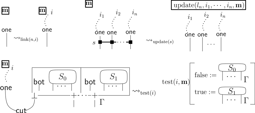
Figure 6: Program Net Reduction Involving Memories.

• Link. If $n$ is a $\mathsf{one}$ node of conclusion $x$, with ${\tt ind}_{R}(x)$ undefined, then $(R,{\tt ind}_{R},\mathbf{m})\rightsquigarrow_{\mathrm{link(n,i)}}\{(R,{\tt ind}_{R}\cup\{x\mapsto i\},\mathbf{m})^{1}\}$ where $i\in I$ is fresh both in ${\tt ind}_{R}$ and $\mathbf{m}$.

• Update. If $R\rightsquigarrow_{s}R^{\prime}$, and $s$ is the sync node in the redex, then

  $$(R,{\tt ind}_{R},\mathbf{m})\rightsquigarrow_{\mathrm{update(s)}}\{(R^{\prime},{\tt ind}_{R},\mathrm{update}(l,\vec{i},\mathbf{m})^{1}\}$$

  where $l$ is the label of $s$, and $\vec{i}$ are the addresses of its premises.

• Test. If $R\rightsquigarrow_{u_{0}}R_{0}$ and $R\rightsquigarrow_{u_{1}}R_{1}$, and $i$ is the address of the premise $\mathsf{1}$ of the cut, then $(R,{\tt ind}_{R},\mathbf{m})\rightsquigarrow_{\mathrm{test(i)}}$ $\mathrm{test}(i,\mathbf{m})[{\rm false}{:}{=}(R_{0},{\tt ind}_{R_{0}},\mathbf{m}),$ ${\rm true}{:}{=}(R_{1},$ ${\tt ind}_{R_{1}},\mathbf{m})]$, where ${\tt ind}_{R_{0}}$ (resp. ${\tt ind}_{R_{1}}$) is the restriction of ${\tt ind}_{R}$ to ${\tt Inputs}(R_{0})$ (resp. ${\tt Inputs}(R_{1})$).

• Otherwise, if $R\rightsquigarrow_{x}R^{\prime}$ with $x\not\in\{s,u_{0},u_{1}\}$, then we have

  $$(R,{\tt ind}_{R},\mathbf{m})\rightsquigarrow_{x}\{(R^{\prime},{\tt ind}_{R},\mathbf{m})^{1}\}$$

  (observe that none of these rules modify the domain of ${\tt ind}_{R}$).

The relation $\rightsquigarrow$ extends immediately to program nets (by slight abuse of notation we use the same symbol); Lem. 17 guarantees that the relation is well defined. We write $(R,{\tt ind}_{R},\mathbf{m})\stackrel{{\scriptstyle r}}{{\rightsquigarrow}}\mu$ for the reduction of the redex $r$ in the raw program net $(R,{\tt ind}_{R},\mathbf{m})$.

Lemma 17 (Reduction Preserves Equivalence).

Suppose that $(R,{\tt ind}_{R},\mathbf{m})\stackrel{{\scriptstyle r}}{{\rightsquigarrow}}\mu$ and $(R,\sigma\cdot{\tt ind}_{R},\sigma\cdot\mathbf{m})\stackrel{{\scriptstyle r}}{{\rightsquigarrow}}\nu$, then $\mu\sim\nu$.

Proof.

Let us check the rule $\rightsquigarrow_{{\rm test}(i)}$. Suppose $(R^{\prime},{\tt ind}_{R^{\prime}},\mathbf{m}^{\prime})=\sigma(R,{\tt ind}_{R},\mathbf{m})$, $(R,{\tt ind}_{R},\mathbf{m})\stackrel{{\scriptstyle r}}{{\rightsquigarrow}}_{{\rm test}\!(\!i\!)}\mu\,{=}\,\{(R_{0},{\tt ind}_{R_{0}},\mathbf{m}_{0})^{p_{0}}\!,$ $(R_{1},{\tt ind}_{R_{1}},\mathbf{m}_{1})^{p_{1}}\}$, and $(R^{\prime},{\tt ind}_{R}^{\prime},\mathbf{m}^{\prime})\stackrel{{\scriptstyle r}}{{\rightsquigarrow}}_{{\rm test}(i)}$

$\nu=\{(R_{0}^{\prime},{\tt ind}_{R_{0}}^{\prime},\mathbf{m}_{0}^{\prime})^{p_{0}^{\prime}},(R_{1}^{\prime},{\tt ind}_{R_{1}^{\prime}},\mathbf{m}_{1}^{\prime})^{p_{1}^{\prime}}\}$ by reducing the same redex $r$. It suffices to show that $\nu=\sigma\cdot\mu$. Element-wise, we have to check $R_{i}^{\prime}=R_{i}$, ${\tt ind}_{R_{i}}^{\prime}=\sigma\circ{\tt ind}_{R_{i}}^{\prime}$, $\mathbf{m}_{i}^{\prime}=\sigma\cdot\mathbf{m}_{i}$, and $p_{i}^{\prime}=p_{i}$ for $i\in\{0,1\}$. The first two follow by definition of $\rightsquigarrow_{{\rm test}(i)}$ and the last two follow from the equation $\sigma\cdot({\rm test}(i,m))={\rm test}(\sigma(i),\sigma\cdot m)$. The other rules can be similarly checked. ∎

Remark 18.

In the definition of the reduction rules:

• Link is independent from the choice of $i$. If we chose another address $j$ with the same conditions, then we would have gone to $(R,{\tt ind}_{R}\cup\{x\mapsto j\},\mathbf{m})$. However this does not cause a problem: by using a permutation $\sigma=(i~{}j)$, since $\sigma\cdot\mathbf{m}=\mathbf{m}$ we have $\sigma(R,{\tt ind}_{R}\cup\{x\mapsto i\},\mathbf{m})=(R,{\tt ind}_{R}\cup\{x\mapsto j\},\mathbf{m})$ and therefore $(R,{\tt ind}_{R}\cup\{x\mapsto i\},\mathbf{m})$ and $(R,{\tt ind}_{R}\cup\{x\mapsto j\},\mathbf{m})$ are as expected the exact same program net.

• In the rules Update and Test, the involved $\mathsf{one}$ nodes are required to be active.

The pair $(\mathcal{N},\rightsquigarrow)$ forms a PARS. Reduction can happen at different places in a net, however the diamond property allows us to deal with this seamlessly.

Figure 7: Example of Program Net Rewriting.

Proposition 19 (Program Nets are Diamond).

The PARS $(\mathcal{N},\rightsquigarrow)$ satisfies the diamond property.∎

The proof (see Appendix B) relies on commutativity of the memory operations. Due to Th. 11, program net reduction enjoys all the good properties we have studied in Sec. 2:

Corollary 20.

The relation $\rightsquigarrow$ satisfies Confluence, Uniformity and Uniqueness of Normal Forms (see Th. 11). ∎

The following two results can be obtained as adaptations of similar ones in Dal Lago et al. [2015].

Theorem 21 (Deadlock-Freeness of Net Reduction).

Let $\mathbf{R}=[(R,{\tt ind}_{R},$ $\mathbf{m})]$ be a program net such that no $\bot$, $?$ or $!$ appears in the conclusions of the net $R$. If $R$ contains cuts, a reduction step is always possible.∎

Corollary 22 (Cut Elimination).

With the same hypothesis as above, if $\mathbf{R}\not\rightsquigarrow$, (i.e. no further reduction is possible) then $\mathbf{R}$ is cut free.∎

Example.

The net in LHS of Fig. 5 can be embedded into a program net with a quantum memory of empty support: $(0,0,0,\ldots)\equiv{}$ “$|{000\ldots}\rangle$”. It reduces according to Fig. 5, with the same memory. The next step requires a $\rightsquigarrow_{\mathrm{link}}$-rewrite step to attach a fresh address—say, $0$—to the $\mathsf{one}$ node at surface. The $\mathsf{H}$-sync node then rewrites with a $\rightsquigarrow_{\mathrm{update}}$-step, and we get the program net (A) in Fig. 7 with the “update” action applied to the memory: the memory corresponds to $\frac{\sqrt{2}}{2}(|{0}\rangle+|{1}\rangle)\otimes|{00\ldots}\rangle$. From there, a choice reduction is in order: it uses the “test” action of the memory structure, which, according to Sec. 3.3.3 corresponds to the measurement of the qubit at address $0$. This yields the probabilistic superposition of the program nets (B₁) and (B₂). As the net in (B₁) is the LHS of Fig. 5, it reduces to (C₁) (dashed arrow (a)), similar to (A) modulo the fact that the address $0$ was not fresh: the $\rightsquigarrow_{\mathrm{link}}$-rewrite step cannot yield $0$: here we choose $1$. Note that we could have chosen any other non-zero number as the address. The program net (B₂) rewrites to (C₂) (dashed arrow (b)): the weakening node erases the Y-box, and a fresh variable is allocated. In this case, the address 0 is indeed fresh and can be picked.

5 A Memory-Based Abstract Machine

In this section we introduce a class of memory-based token machines, called the MSIAM (Memory-based Synchronous Interaction Abstract Machine). The base rewrite system on which the MSIAM is built, is a variation of the SIAM multi-token machine from Dal Lago et al. [2015], which we recall in Sec. 5.1. The specificity of the SIAM is to allow not only parallel threads, but also interaction among them, i.e. synchronization. Synchronization happens in particular at the sync nodes (unsurprisingly, as these are nodes introduced with this purpose), but also on the additive boxes (the $\bot$-box). The transitions at the $\bot$-box model choice: as we see below, when the flow of computation reaches the $\bot$-box (i.e. the tokens reach the auxiliary doors), it continues on one of the two sub-components, depending on the tokens which are positioned at the principal door.

The original contribution of this section is contained in Sections  5.2 through  5.4, where we use our parametric construction to define the MSIAM $\mathcal{M}_{\mathbf{R}}$ for $\mathbf{R}$ as a PARS consisting of a set of states $\mathcal{S}$, and a transition relation $\mathord{\rightarrow}\subset\mathcal{S}\times\mathit{DST}(\mathcal{S})$, and establish its main properties, in particular Deadlock-Freeness (Th. 26), Invariance (Th. 27) and Adequacy (Th. 28).

5.1 SIAM

Let $R$ be a net. The SIAM for $R$ is given by a set of states and a transition relation on states. Most of the definitions are standard.

Exponential signatures $\sigma$ and stacks $s$ are defined by
$\begin{array}[]{l@{~}l@{~}l}\sigma\mathrel{::=}{*}\mid l(\sigma)\mid r(\sigma)\mid\lceil\sigma,\sigma\rceil\mid y(\sigma,\sigma)\hfil~{}\\ \mathord{s}\mathrel{::=}\epsilon\mid l.\mathord{s}\mid r.\mathord{s}\mid\sigma.\mathord{s}\mid\delta\hfil~{}\end{array}$
where $\epsilon$ is the empty stack and . denotes concatenation. Two kinds of stacks are defined: (1.) the formula stack and (2.) the box stack. The latter is the standard GoI way to keep track of the different copies of a box. The former describes the formula path of either an occurrence $\alpha$ of a unit, or an occurrence $\Diamond$ of a modality, in a formula $A$. Formally, $\mathord{s}$ is a formula stack on $A$ if either $\mathord{s}=\delta$ or $\mathord{s}[A]=\alpha$ (resp. $\mathord{s}[A]=\Diamond$), with $\mathord{s}[A]$ defined as follows: $\epsilon[\alpha]=\alpha$, $\sigma.\delta[\Diamond B]={\Diamond}$, $\sigma.t[\Diamond B]=t[B]$ whenever $t\neq\delta$, $l.t[B\Box C]=t[B]$ and $r.t[B\Box C]=t[C]$ (where $\Box$ is either $\otimes$ or $\parr$). We say that $\mathord{s}$ indicates the occurrence $\alpha$ (resp. $\Diamond$).

Example 23.

Given the formula $A=\mathop{!}\nolimits(\bot\otimes{!\mathsf{1}})$, the stack $*.\delta$ indicates the leftmost occurrence of $\mathop{!}\nolimits$, the stack ${*}.r.{*}.\delta$ indicates the rightmost occurrence of $!$, and $*.l[A]=\bot$.

Positions.

Given a net $R$, the set of its positions $\mathtt{POS}_{R}$ contains all the triples $(\mathord{e},\mathord{s},\mathord{t})$, where $\mathord{e}$ is an edge of $R$, $\mathord{s}$ is a formula stack on the type $A$ of $\mathord{e}$, and $\mathord{t}$ (the box stack) is a stack of $n$ exponential signatures, where $n$ is the depth of $\mathord{e}$ in $R$. We use the metavariables $\mathbf{s}$ and $\mathbf{p}$ to indicate positions. For each position $\mathbf{p}=(\mathord{e},\mathord{s},\mathord{t})$, we define its direction $\mathrm{dir}(\mathbf{p})$ to be upwards ($\uparrow$) if $\mathord{s}$ indicates an occurrence of $!$ or $\bot$, to be downwards ($\downarrow$) if $\mathord{s}$ indicates an occurrence of $?$ or $\mathsf{1}$, to be stable ($\leftrightarrow$) if $\mathord{s}=\delta$ or if the edge $\mathord{e}$ is the conclusion of a $\mathsf{bot}$ node. The following subsets of $\mathtt{POS}_{R}$ play a role in the definition of the machine:

• the set $\mathtt{INIT}_{R}$ of initial positions $\mathbf{p}=(\mathord{e},\mathord{s},\epsilon)$, with $e$ conclusion of $R$, and $\mathrm{dir}(\mathbf{p})$ is $\uparrow$;

• the set $\mathtt{FIN}_{R}$ of final positions $\mathbf{p}=(\mathord{e},\mathord{s},\epsilon)$, with $e$ conclusion of $R$, and $\mathrm{dir}(\mathbf{p})$ is $\downarrow$;

• the set $\mathtt{ONES}_{R}$ of positions $(\mathord{e},\epsilon,\mathord{t})$, $\mathord{e}$ conclusion of a $\mathsf{one}$ node;

• the set $\mathtt{DER}_{R}$ of positions $(\mathord{e},*.\delta,\mathord{t})$, $\mathord{e}$ conclusion of a $\mathsf{?d}$ node;

• the set $\mathtt{STABLE}_{R}$ of the positions $\mathbf{p}$ for which $\mathrm{dir}(\mathbf{p})={\leftrightarrow}$;

• the set of starting positions $\mathtt{START}_{R}=\mathtt{INIT}_{R}\cup\mathtt{ONES}_{R}\cup\mathtt{DER}_{R}$.

SIAM States.

A state $(T,\mathrm{orig})$ of $\mathcal{M}_{R}$ is a set of positions $T\subseteq\mathtt{POS}_{R}$ equipped with an injective map $\mathrm{orig}:T\to\mathtt{START}_{R}$. Intuitively, $T$ describes the current positions of the tokens, and $\mathrm{orig}$ keeps track of where each such token started its path.

A state is initial if $T\subseteq\mathtt{INIT}_{R}$ and $\mathrm{orig}$ is the identity. We indicate the (unique) initial state of $\mathcal{M}_{R}$ by $I_{R}$. A state $T$ is final if all positions in $T$ belong to either $\mathtt{FIN}_{R}$ or $\mathtt{STABLE}_{R}$.

With a slight abuse of notation, we will denote the state $(T,\mathrm{orig})$ also by $T$. Given a state $T$ of $\mathcal{M}_{R}$, we say that there is a token in $\mathbf{p}$ if $\mathbf{p}\in T$. We use expressions such as “a token moves”, “crosses a node”, in the intuitive way.

SIAM Transitions.

The transition rules of the SIAM are described in Fig. 8 and 9. Rules (i)-(iv) require synchronization among different tokens; this is expressed by specific multi-token conditions which we discuss in the next paragraph. First, we explain the graphical conventions and give an overview of the rules.

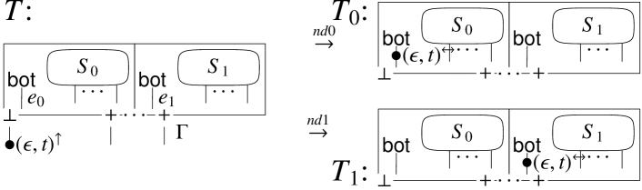
Figure 8: SIAM  Non-Deterministic Transition Rules.

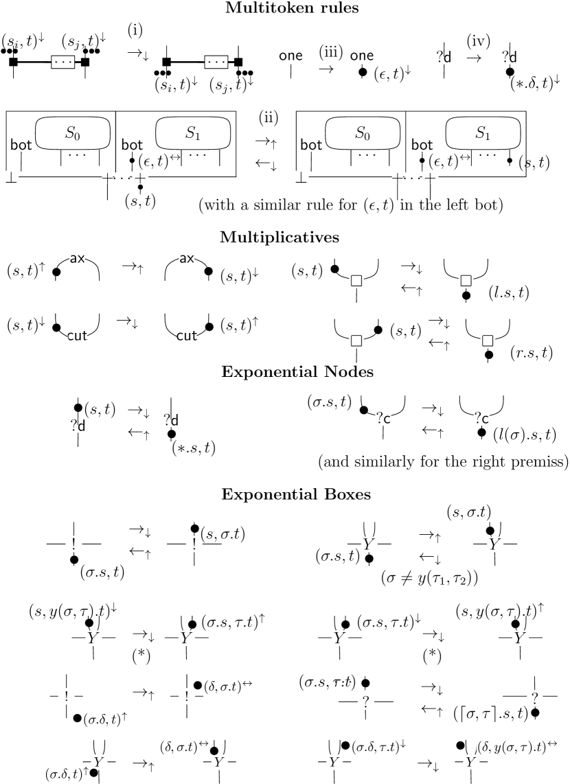
Figure 9: SIAM: Deterministic Transition Rules.

The position $\mathbf{p}=(\mathord{e},\mathord{s},\mathord{t})$ is represented graphically by marking the edge $e$ with a bullet $\bullet$, and writing the stacks $(\mathord{s},\mathord{t})$. A transition $T\rightarrow U$ is given by depicting only the positions in which $T$ and $U$ differ. It is intended that all positions of $T$ which do not explicitly appear in the picture also belong to $U$. To save space, in Fig. 9 the transition arrows are annotated with a direction; this means that the rule applies (only) to positions which have that direction. When useful, the direction of a position is directly annotated with ${}^{\downarrow},{}^{\uparrow}$ or ^↔. Note that no transition is defined for stable positions. For boxes, whenever a token is on a conclusion of a box, it can move into that box (graphically, the token “crosses” the border of the box) and it is modified as if it were crossing a node. For exponential boxes, Fig. 9 depicts only the border of the box. We do not explicitly give the function $\mathrm{orig}$, which is immediate to reconstruct when keeping in mind that it is a pointer to the origin of the token.

We briefly discuss the most interesting transitions (we refer to Dal Lago et al. [2015] for a broader discussion). Fixpoints: the recursive behavior of Y-boxes is captured by the exponential signature in the form $y(\cdot,\cdot)$, and the associated transitions. Duplication: the key is rule (iv), which generates a token on the conclusion of a $\mathsf{?d}$ node; this token will then travel the net, possibly crossing a number of contractions, until it finds its exponential box; intuitively, each such token corresponds to a copy of a box. One: the behavior of the token generated by rule (iii) on the conclusion of a $\mathsf{one}$ node is similar to that of a dereliction token; the $\mathsf{one}$ token searches for its $\bot$-box. Stable tokens: when the token from an instance of a $\mathsf{?d}$ or of a $\mathsf{one}$ node “has found its box”, i.e. it reaches the principal door of a box, the token become stable ($\leftrightarrow$). A stable token is akin to a marker sitting on the principal door of its box, keeping track of the box copies and of the choice made in each specific copy.

Multi-token Conditions.

The rules marked by (i), (ii), (iii), and (iv) in Fig. 9 require the tokens to interact, which is formalized by multi-token conditions. Such conditions allow, in particular, to capture choice and synchronization. Below we give an intuitive presentation; we refer to Dal Lago et al. [2015, 2016] for the formal details. For convenience we also recall them in Appendix C.

Synchronization, rule (i). To cross a sync node $l$, all the positions on the premises of $l$ (for the same box stack $\mathord{t}$) must be filled; intuitively, having the same $\mathord{t}$, means that the positions all belong to the same copy of $l$. Only when all the tokens have reached $l$, they can cross it; they do so simultaneously.

Choice, rule (ii). Any token arriving at a $\bot$-box on an auxiliary door must wait for a token on the principal door to have made a choice for either of the two contents, $S_{0}$ or $S_{1}$: a token $(e,s,t)$ on the conclusions $\Gamma$ of the $\bot$-box will move to $S_{0}$ (resp. $S_{1}$) only if the principal door of $S_{0}$ (resp. $S_{1}$) has a token with the same $\mathord{t}$.

The rules marked by (iii) and (iv) also carry a multi-token condition, but in a more subtle way: a token is enabled to start its journey on a $\mathsf{one}$ or $\mathsf{?d}$ node only when its box has been opened; this reflects in the SIAM the constraint of surface reduction of nets.

5.2 MSIAM

Similarly to what we have done for nets, we enrich the machine with a memory, and use the SIAM and the operations on the memory to define a PARS.

MSIAM States.

Given a memory structure $\mathrm{Mem}=(\mathrm{Mem},I,\mathcal{L})$ and a raw program net $(R,{\tt ind}_{R},\mathbf{m}_{R})$ on $\mathrm{Mem}$, a raw state of the MSIAM $\mathcal{M}_{\mathbf{R}}$ is a tuple $(T,{\tt ind}_{\mathbf{T}},\mathbf{m}_{T})$ where

• $T$ is a state of $\mathcal{M}_{R}$,

• ${\tt ind}_{T}\colon\mathtt{START}_{R}\to I$ is a partial injective map,

• $\mathbf{m}_{T}\in\mathrm{Mem}$.

States are defined as the equivalence class $\mathbf{T}=[(T,{\tt ind}_{T},\mathbf{m}_{T})]$ of row states over permutations, with the action of $\rm Perm(I)$ on tuples being the natural one.

MSIAM Transitions.

Let $\mathbf{R}$ be a program net, and $\mathbf{T}$ be a state $[(T,{\tt ind}_{T},\mathbf{m}_{T})]$ of $\mathcal{M}_{\mathbf{R}}$. We define the transition $\mathbf{T}\rightarrow\mu\in\mathcal{S}\times\mathit{DST}(\mathcal{S})$. As we did for program nets, we first give the definition on raw states. The definition depends on the SIAM transitions for $T$. Let us consider the possible cases.

• Link. Assume $T\stackrel{{\scriptstyle(iii)}}{{\rightarrow}}U$ (Fig. 9), and let $n$ be the $\mathsf{one}$ node, $x$ its conclusion, and $\mathbf{p}$ the new token in $U$. We set

  $$(T,{\tt ind}_{T},\mathbf{m})\rightarrow_{\mathrm{link(n,i)}}(U,{\tt ind}_{T}\cup\{\mathrm{orig}(\mathbf{p})\mapsto i\},\mathbf{m})$$

  where we choose $i={\tt ind}_{R}(x)$ if the $\mathsf{one}$ node is active, and otherwise an address $i$ which is fresh for both ${\tt ind}_{T}$ and $(\mathbf{m})$.

• Update. Assume $T\stackrel{{\scriptstyle(i)}}{{\rightarrow}}U$ (Fig. 9), $l$ is the name associated to the sync node, and $\vec{i}$ are the addresses which are associated to its premises (by composing $\mathrm{orig}{}$ and ${\tt ind}$), then

  $$(T,{\tt ind}_{T},\mathbf{m})\rightarrow_{\mathrm{update(s)}}\{(U,{\tt ind}_{T},\mathrm{update}(l,\vec{i},\mathbf{m})^{1}\}.$$

• Test. Assume $T\stackrel{{\scriptstyle nd0}}{{\rightarrow}}T_{0}$ and $T\stackrel{{\scriptstyle nd1}}{{\rightarrow}}T_{1}$ (Fig. 8, non-deterministic transition). If $\mathbf{p}\in T$ is the token appearing in the redex (Fig. 8), and $i$ the addresses that ${\tt ind}_{T}$ associates to $\mathrm{orig}(\mathbf{p})$, then

  $(T,{\tt ind}_{\mathbf{T}},\mathbf{m})\rightarrow_{\mathrm{test(i)}}$

  $\mathrm{test}(i,\mathbf{m})[{\rm false}:=(T_{0},{\tt ind}_{T}),{\rm true}:=(T_{1},$ ${\tt ind}_{T})]$.

• In all the other cases: if $T\rightarrow U$ then $(T,{\tt ind}_{T},\mathbf{m})\rightarrow\{(U,{\tt ind}_{T},\mathbf{m})^{1}\}.$

Let $\mathbf{R}=[(R,{\tt ind}_{R},\mathbf{m}_{R})]$. The initial state of $\mathcal{M}_{\mathbf{R}}$ is $\mathbf{I}_{\mathbf{R}}=[(I_{R},{\tt ind}_{I_{R}},\mathbf{m}_{R})]$, where ${\tt ind}_{I_{R}}$ is only defined on the initial positions: if $\mathbf{p}\in\mathtt{INIT}_{R}$, and $x$ is the occurrence of $\bot$ corresponding to $\mathbf{p}$, then ${\tt ind}_{I_{R}}(\mathbf{p})={\tt ind}_{R}(x)$. A state $[$$(T,{\tt ind}_{T},\mathbf{m}_{T})$$]$ is final if $T$ is final.

Figure 10: MSIAM run of Fig. 5.

In the next sections, we study the properties of the machine, and show that the MSIAM is a computational model for $\mathcal{N}$.

Example.

We informally develop in Fig. 10 an execution of the MSIAM for the LHS net of Fig. 5. In the first panel (A) tokens (a) and (b) are generated. Token (a) reaches the principal door of the $Y$-box, which corresponds to opening a first copy. Token (b) enters the $Y$-box and hits the $\bot$-box. The test action of the memory triggers a probabilistic distribution of states where the left and the right components of the $\bot$-box are opened: the corresponding sequences of operations are Panels (B₀) and (B₁) for the left and right sides.

In Panel (B₀): the left-side of the $\bot$-box  is opened and its $\mathsf{one}$-node emits the token (c) that eventually reaches the conclusion of the net. In Panel (B₁): the right-side of the $\bot$-box is opened and tokens (c) and (d) are emitted. Token (d) opens a new copy of the $Y$-box, while token (c) hits the $\bot$-box of this second copy. The test action of the memory again spawns a probabilistic distribution.

We focus on panel (C₁₀) on the case of the opening of the left-side of the $\bot$-box: there, a new token (e) is generated. It will exit the second copy of the $Y$-box, go through the first copy and exit to the conclusion of the net.

5.3 MSIAM Properties, and Deadlock-Freeness

Intuitively, a run of the machine $\mathcal{M}_{\mathbf{R}}$ is the result of composing transitions of $\mathcal{M}_{\mathbf{R}}$, starting from the initial state $\mathbf{I}_{\mathbf{R}}$ (composition being transitive composition). We are not interested in the actual order in which the transitions are performed in the various components of a distribution of states. Instead, we are interested in knowing which distributions of states are reached from the initial state. This notion is captured well by the relation $\mathrel{\looparrowright}$ (see Sec. 2.1). We will say that a run of the machine $\mathcal{M}_{\mathbf{R}}$ reaches $\mu\in\mathit{DST}(\mathcal{S}_{\mathbf{R}})$ if $\mathbf{I}_{\mathbf{R}}\mathrel{\looparrowright}\mu$. We will also use the expression “a run of $\mathcal{M}_{\mathbf{R}}$ reaches a state $\mathbf{T}$” if $\mathbf{I}\mathrel{\looparrowright}\mu$ with $T\in\mathit{SUPP}(\mu)$.

An analysis similar to the one done for program nets shows the next lemma (Lem. 24) and therefore Prop. 25:

Lemma 24 (Diamond).

The relation $\rightarrow$ satisfies the diamond property.∎

Proposition 25 (Confluence, Uniqueness of Normal Forms, Uniformity).

The relation $\rightarrow$ satisfies confluence, uniformity, and uniqueness of normal forms.∎

By the results we have studied in Sec. 2, we thus conclude that all runs of $\mathcal{M}_{\mathbf{R}}$ have the same behavior with respect to the degree of termination, i.e. if $\mathbf{I}_{\mathbf{R}}$ p-normalizes following a certain sequence of reductions, it will do so whatever sequence of reductions we pick. We say that the machine $\mathcal{M}_{\mathbf{R}}$ $p$-terminates if $\mathbf{I}_{\mathbf{R}}$ $p$-terminates (see Def. 4).

Deadlocks.

A terminal state $\mathbf{T}\nrightarrow$ of $\mathcal{M}_{\mathbf{R}}$ can be final or not. A non-final terminal state is called a deadlocked state. Because of the inter-dependencies among tokens given by the multi-token conditions, a multi-token machine is likely to have deadlocks. We are however able to guarantee that any MSIAM machine is deadlock-free, whatever is the choice for the memory structure.

Theorem 26 (Deadlock-Freeness of the MSIAM).

Let $\mathbf{R}$ be a program net of conclusion $\mathsf{1}$; if $\mathbf{I}_{\mathbf{R}}\mathrel{\looparrowright}\mu$ and $\mathbf{T}\in\mathit{SUPP}(\mu)$ is terminal, then $\mathbf{T}$ is a final state.∎

The proof (see Appendix D.3) relies on the diamond property of the machine (more precisely, uniqueness of the normal forms).

5.4 Invariance and Adequacy

The machine $\mathcal{M}_{\mathbf{R}}$ gives a computational semantics to $\mathbf{R}$. The semantics is invariant under reduction (Th. 27); the adequacy result (Th. 28) relates convergence of the machine and convergence of the nets. We define the convergence of the machine as the convergence of its initial state:

$\mathcal{M}_{\mathbf{R}}\Downarrow_{p}$ if $\mathbf{I}_{\mathbf{R}}$ converges with probability $p$ (i.e. $\mathbf{I}_{\mathbf{R}}\Downarrow_{p}$).

Theorem 27 (Invariance).

Let $\mathbf{R}$ be a program net of conclusion $\mathsf{1}$. Assume $\mathbf{R}\rightsquigarrow\sum_{i}{p_{i}}\cdot\{\mathbf{R}_{i}\}$. Then we have that $\mathcal{M}_{\mathbf{R}}\Downarrow_{q}$ if and only if $\mathcal{M}_{\mathbf{R}_{i}}\Downarrow_{q_{i}}$ with $\sum_{i}(p_{i}\cdot q_{i})=q$.∎

Theorem 28 (Adequacy).

Let $\mathbf{R}$ be a program net of conclusion $\mathsf{1}$. Then, $\mathcal{M}_{\mathbf{R}}\Downarrow_{p}$ if and only if $\mathbf{R}\Downarrow_{p}$.∎

The proofs of invariance and adequacy, are both based on the diamond property of the machine, and on a map—which we call transformation—which allows us to relate the rewriting of program nets with the MSIAM. To obtain the proofs, we need to establish a series of technical results which we give in Appendix  D.

6 A $\mathsf{PCF}$-style Language with Memory Structure

We introduce a $\mathsf{PCF}$-style language which is equipped with a memory structure, and is therefore parametric on it. The base type will correspond to elements stored in the memory, and the base operations to the operations of the memory structure.

6.1 Syntax and Typing Judgments

The language $\mathsf{PCF}^{\mathsf{LL}}$ which we propose is based on Linear Logic, and is parameterized by a choice of a memory structure $\mathrm{Mem}$.

The terms ($M,N,P$) and types ($A,B$) are defined as follows:

$$\begin{array}[]{@{}l@{~}l@{~}l@{}}M,N,P\hfil~{}&{:}{:}{=}\hfil~{}&x\,|\,\lambda x.M\,|\,MN\,|\,{{\tt let}\,{\langle}{x,y}{\rangle}={M}\,{\tt in}\,{N}}\,|\,{\langle{M,N}\rangle}\,|\\ \hfil~{}&\hfil~{}&{{\tt letrec}\,{f}\,{x}={M}\,{\tt in}\,{N}}\,|\\ \hfil~{}&\hfil~{}&{\tt new}\,|\,{\tt c}\,|\,{{\tt if}\,{P}\,{\tt then}\,{M}\,{\tt else}\,{N}},\\ A,B\hfil~{}&{:}{:}{=}\hfil~{}&\alpha\,|\,A\multimap B\,|\,A\otimes B\,|\,{!}A\end{array}$$

where ${\tt c}$ ranges over the set of memory operations $\mathcal{L}$. A typing context $\Delta$ is a (finite) set of typed variables $\{x_{1}:A_{1},\dots,x_{n}:A_{n}\}$, and a typing judgment is written as $\Delta\vdash M:A.$ An empty typing context is denoted by “$\cdot$”. We say that a type is linear if it is not of the form ${!}A$. We denote by ${!}\Delta$ a typing context with only non-linearly typed variables. A typing judgment is valid if it can be derived from the set of typing rules presented in Fig. 11. We require $M$ and $N$ to have empty context in the typing rule of ${{\tt if}\,{P}\,{\tt then}\,{M}\,{\tt else}\,{N}}$. The requirement does not reduce expressivity as typing contexts can always be lambda-abstracted. The typing rules make use of a notion of values, defined as follows: $U,V~{}{:}{:}{=}~{}x\,|\,\lambda x.M\,|\,{\langle{U,V}\rangle}\,|\,{\tt c}$.

$$\begin{array}[]{c}{!}\Delta\vdash{\tt new}:\alpha\quad{!}\Delta,x:{!}(A\multimap B)\vdash x:A\multimap B\quad{!}\Delta,x:A\vdash x:AA\textrm{ linear}\quad{!}\Delta\vdash V:{!}(A\multimap B)\lx@proof@logical@and{!}\Delta\vdash V:A\multimap BV\textrm{ value}\quad\Delta\vdash\lambda x.M:A\multimap B\Delta,x:A\vdash M:B\\[4.30554pt] {!}\Delta,\Gamma_{1},\Gamma_{2}\vdash MN:B\lx@proof@logical@and{!}\Delta,\Gamma_{1}\vdash M:A\multimap B{!}\Delta,\Gamma_{2}\vdash N:A\,\,{!}\Delta,\Gamma_{1},\Gamma_{2}\vdash{{\tt let}\,{\langle}{x,y}{\rangle}={M}\,{\tt in}\,{N}}:C\lx@proof@logical@and{!}\Delta,\Gamma_{1}\vdash M:A\otimes B{!}\Delta,\Gamma_{2},x:A,y:B\vdash N:C\,\,\,{!}\Delta,\Gamma_{1},\Gamma_{2}\vdash{\langle{M,N}\rangle}:A\otimes B\lx@proof@logical@and{!}\Delta,\Gamma_{1}\vdash M:A{!}\Delta,\Gamma_{2}\vdash N:B\\[4.30554pt] \Delta\vdash{{\tt if}\,{P}\,{\tt then}\,{M}\,{\tt else}\,{N}}:A\lx@proof@logical@and\Delta\vdash P:\alpha\cdot\vdash M:A\cdot\vdash N:A\quad{!}\Delta\vdash{\tt c}:\alpha^{\otimes n}\multimap\alpha^{\otimes n}{\rm arity}({\tt c})=n\quad{!}\Delta,\Gamma\vdash{{\tt letrec}\,{f}\,{x}={M}\,{\tt in}\,{N}}:C\lx@proof@logical@and{!}\Delta,f:{!}(A{\multimap}B),x:A\vdash M:B{!}\Delta,\Gamma,f:{!}(A{\multimap}B)\vdash N:C\end{array}$$

Figure 11: Typing Rules.

6.2 Operational Semantics

The operational semantics for $\mathsf{PCF}^{\mathsf{LL}}$ is similar to the one of Pagani et al. [2014], and is inherently call-by-value. Indeed, being based on Linear Logic, the language only allows the duplication of “!”-boxes, that is, normal forms of “!”-type: these are the values. The operational semantics is in the form of a PARS, written $\to$.

The PARS is defined using a notion of reduction context $C[-]$, defined by the grammar

$$\begin{array}[]{@{}l@{~~}l@{~~}l@{}}C[-]\hfil~{}~{}&{:}{:}{=}\hfil~{}~{}&[-]\,|\,C[-]N\,|\,VC[-]\,|\,{\langle{C[-],N}\rangle}\,|\,{\langle{V,C[-]}\rangle}\\ \hfil~{}~{}&\hfil~{}~{}&\,|\,{{\tt let}\,{\langle}{x,y}{\rangle}={C[-]}\,{\tt in}\,{N}}\,|\,{{\tt if}\,{C[-]}\,{\tt then}\,{M}\,{\tt else}\,{N}},\end{array}$$

and a notion of abstract machine: the $\mathsf{PCF}_{\mathsf{AM}}$. A raw $\mathsf{PCF}_{\mathsf{AM}}$ closure is a tuple $(M,{\tt ind}_{M},\mathbf{m})$ where $M$ is a term, ${\tt ind}_{M}$ is an injective map from the set of free variables of $M$ to $I$, and $\mathbf{m}\in\mathrm{Mem}$. $\mathsf{PCF}_{\mathsf{AM}}$ closures are defined as equivalence classes of raw $\mathsf{PCF}_{\mathsf{AM}}$ closures over permutations of addresses.

$$\begin{array}[]{c}(C[{\tt new}],{\tt ind},\mathbf{m})\to_{\mathrm{link}}(C[x],{\tt ind}\cup\{x\mapsto i\},\mathbf{m})\quad(C[{\tt c}\,{\langle{x_{1},\ldots,x_{n}}\rangle}],{\tt ind},\mathbf{m})\to_{\mathrm{update}({\tt c})}(C[{\langle{\vec{x}}\rangle}],{\tt ind},{\rm update}(\vec{i},{\tt c},\mathbf{m}))\\[4.30554pt] (C[{{\tt if}\,{x}\,{\tt then}\,{M_{{\tt t\!\!t}}}\,{\tt else}\,{M_{{\tt f\!\!f}}}}],{\tt ind},\mathbf{m})\to_{\mathrm{test}(i)}{\rm test}(i,\mathbf{m})[{\rm true}:=(M_{{\tt t\!\!t}},{\tt ind}\setminus\{x\mapsto i\}),{\rm false}:=(M_{{\tt f\!\!f}},{\tt ind}\setminus\{x\mapsto i\})]\\[4.30554pt] (C[(\lambda x.M)U],{\tt ind},\mathbf{m})\to(C[M\{x:=U\}],{\tt ind},\mathbf{m})\,\,\,(C[{{\tt let}\,{\langle}{x,y}{\rangle}={{\langle{U,V}\rangle}}\,{\tt in}\,{M}}],{\tt ind},\mathbf{m})\to(C[N[x:=U,y:=V]],{\tt ind},\mathbf{m})\\[4.30554pt] (C[{{\tt letrec}\,{f}\,{x}={M}\,{\tt in}\,{N}}],{\tt ind},\mathbf{m})\to(C[N\{f:=\lambda x.{{\tt letrec}\,{f}\,{x}={M}\,{\tt in}\,{M}}\}],{\tt ind},\mathbf{m})\end{array}$$

Figure 12: Rewrite System for $\mathsf{PCF}_{\mathsf{AM}}$.

The rewrite system is defined in Fig. 12. First, the creation of a new base type element ($\to_{\mathrm{link}}$) is simply memory allocation: $x$ is fresh (and not bound) in $C$ and $i$ is a new address neither in the image of ${\tt ind}$ nor in the support of $\mathbf{m}$. Then, the operation ${\tt c}$ reduces through $\to_{\mathrm{update}({\tt c})}$ using the update of the memory when ${\rm arity}({\tt c})=n$ and ${\tt ind}(x_{k})=i_{k}$. Then, the if-then-else reduces through $\to_{\mathrm{test}(i)}$ using the test operation where ${\tt ind}(x)=i$. Note how we remove $x$ from the domain of ${\tt ind}$. Finally we have the three rules that do not involve probabilities: Note how the mapping ${\tt ind}$ can be kept the same: the set of free variables is unchanged.

Let $\textbf{M}=[(M,{\tt ind},\mathbf{m})]$ be a $\mathsf{PCF}_{\mathsf{AM}}$ closure. We define the judgment $x_{1}:A_{1},\ldots,x_{m}:A_{m}\vdash\textbf{M}:B$ if none of the $x_{i}$’s belongs to ${\rm Dom}({\tt ind})$, $y_{1}:\alpha,\ldots,y_{k}:\alpha,x_{1}:A_{1},\ldots,x_{m}:A_{m}\vdash M:B$, and $\{y_{1},\ldots,y_{k}\}={\rm Dom}({\tt ind})$.

6.3 Modeling $\mathsf{PCF}^{\mathsf{LL}}$ with Nets

We now encode $\mathsf{PCF}^{\mathsf{LL}}$ typing judgments and typed $\mathsf{PCF}_{\mathsf{AM}}$ closures into program nets. As the type system is built on top of Linear Logic, the translation ${(-)}^{\dagger}$ is rather straightforward, modulo one subtlety: it is parameterized by a memory structure $\mathbf{m}$ and a partial function ${\tt ind}$ mapping term variables to addresses in $I$.

The mapping $(-)^{\dagger}$ of types to formulas is defined by $\alpha^{\dagger}~{}{:}{=}~{}\mathsf{1}$, $(A\multimap B)^{\dagger}~{}{:}{=}~{}{(A^{\dagger}{}^{\bot}\parr B^{\dagger})}$ and $(A\otimes B)^{\dagger}~{}{:}{=}~{}{A^{\dagger}}\otimes{B^{\dagger}}$. Now, assume that $\{y_{1},\ldots,y_{n}\}\cap{\rm Dom}({\tt ind})=\emptyset$, that $\Delta$ is a judgment whose variables are all of type $\alpha$, and that $|\Delta|={\rm Dom}({\tt ind})$. The typing judgment $y_{1}:A_{1},\ldots,y_{n}:A_{n},\Delta\vdash M:A$ is mapped through ${(-)}^{\dagger}_{{\tt ind},\mathbf{m}}$ to a program net ${M}^{\dagger}_{{\tt ind},\mathbf{m}}=[(R_{M},{\tt ind}_{R_{M}},\mathbf{m})]$ with conclusions $(A_{1}^{\dagger})^{\bot}$,…$(A_{n}^{\dagger})^{\bot}$, $(B^{\dagger})$ and memory state $\mathbf{m}$ (note how the variables in $\Delta$ do not appear as conclusions). The full definition is found in Appendix E.

6.3.1 Adequacy

As in Sec. 2 and 5.4, given a $\mathsf{PCF}_{\mathsf{AM}}$ closure M we write $\textbf{M}\Downarrow_{p}$ (M converges to $p$) if $p=\mathrm{sup}_{\textbf{M}\mathrel{{\mathrel{\rightrightarrows}}^{*}}\mu}\mathcal{T}(\mu)$. The adequacy theorem then relates convergence of programs and convergence of nets. A sketch of the proof is given in Appendix E.

Theorem 29.

Let $\vdash\textbf{M}:\alpha$, then $\textbf{M}\,{\Downarrow_{p}}$ if and only if ${\textbf{M}}^{\dagger}{\Downarrow_{p}}$.∎

7 Results and Discussion

As we anticipated in Sec. 1.3, we have proved—parametrically on the memory—that the MSIAM is an adequate model of program nets reduction (Th. 28), and program nets are expressive enough to adequately represent the behavior of the $\mathsf{PCF}^{\mathsf{LL}}$ abstract machine (Th. 29). What does this mean? As soon as we choose a concrete instance of memory structure, we have a language and an adequacy result for it. This is in particular the case for all instances of memory which are outlined in Sec. 3.3. To make this explicit, let $\mathcal{I}$, $\mathcal{P}$ and $\mathcal{Q}$ be respectively a deterministic, probabilistic and quantum memory. We denote by $\mathsf{PCF}^{\mathsf{LL}}$($\mathcal{I}$), $\mathsf{PCF}^{\mathsf{LL}}$($\mathcal{P}$) and $\mathsf{PCF}^{\mathsf{LL}}$($\mathcal{Q}$), respectively, the language which is obtained by choosing that memory. Observe in particular that the choice of $\mathcal{P}$ or $\mathcal{Q}$, respectively specialize our adequacy result into a semantics for a probabilistic $\mathsf{PCF}$  in the style of Ehrhard et al. [2014], and a semantics for a quantum $\mathsf{PCF}$, in the style of Selinger and Valiron [2006]; Pagani et al. [2014].

7.1 The Quantum Lambda Calculus

Let us now focus on the quantum case, and analyze in some depth our result. We have a quantum lambda-calculus, namely $\mathsf{PCF}^{\mathsf{LL}}$($\mathcal{Q}$), together with an adequate multi-token semantics. How does our calculus relate with the ones in the literature?

We first observe that the syntax of $\mathsf{PCF}^{\mathsf{LL}}$($\mathcal{Q}$) is very close to the language of Pagani et al. [2014] (we only omit lists and coproducts). The operational semantics is also the same, as one can easily see. Indeed, the abstract machine in Pagani et al. [2014] consists of a triple $(Q,L,M)$ where $M$ is a lambda-term and where $Q$ and $L$ are as presented in Sec. 3.3.3. As we discussed there, for $Q$ and $L$ one can use either the canonical presentation of Pagani et al. [2014], or the memory structure $\mathcal{Q}$.

7.1.1 Discussion on the Quantum Model

It is now time to go back to the programs in our motivating examples, Examples 2 and 3. Both programs are valid terms in $\mathsf{PCF}^{\mathsf{LL}}$($\mathcal{Q}$); we have already informally developed Example 3 within our model.

We claimed in the Introduction that Example 2 cannot be represented in the GoI model described in Hasuo and Hoshino [2011]: the reason is that the model does not support entangled qubits in the type $\alpha\otimes\alpha$ (using our notation), a tensor product is always separable. To handle entangled states, Hasuo and Hoshino [2011] uses non-splittable, crafted types: this is why the simple term in Example 2 is forbidden. In the MSIAM, entangled states pose no problem, as the memory is disconnected from the types.

The term of Example 3, valid in $\mathsf{PCF}^{\mathsf{LL}}$($\mathcal{Q}$), is mapped through $(-)^{\dagger}$ to the net of Fig. 5: Th. 29 and 28 state that the corresponding MSIAM presented in Fig. 10 is adequate. Note that Example 3 was presented in the context of quantum computation. It is however possible (and the behavior is going to be the same as the one already described) to use the probabilistic memory sketched in Sec. 3.3.2. In this case, the $\mathsf{H}$-sync node would be changed for the coin-sync node.

7.1.2 Qubits, Duplication and Erasing

It is worth to pinpoint the technical ingredients which allow for the coexistence of quantum bits with duplication and erasing. In the language, the reason is that, similarly to Pagani et al. [2014], $\mathsf{PCF}^{\mathsf{LL}}$ allows only lambda-abstractions (or tuples thereof) to be duplicated. In the case of the nets (and therefore of the MSIAM), the key ingredient is surface reduction (Sec. 4.2): the allocation of a quantum bit is captured by the link rule which associates a $\mathsf{one}$ node to the memory. Since a $\mathsf{one}$ node linked to the memory cannot lie inside a box, it will never be copied nor erased. Indeed, the ways in which the language and the model deal with quantum bits, actually match.

7.1.3 More Possibilities for Quantum Memory Structure

In the presentation of $\mathcal{Q}$ we have given in Sec. 3.3.3, fresh qubits were arbitrarily created in state $|{0}\rangle$. We could as well have chosen, say, $|{1}\rangle$ for default value. Formally, if we want to do that we can use the set $\mathcal{F}_{1}$ of (set-)maps from $I$ to $\{0,1\}$ that have value $1$ everywhere except for a finite subset of $I$. The structure $\mathcal{Q}$ would then have been defined as $\mathcal{H}_{1}$, the Hilbert space built from finite linear combinations of $\mathcal{F}_{1}$.

Unlike the case of the integer memory, the mathematical properties of quantum states can make the test action modify the state of the fresh addresses. Let us see how this happens.

Indeed, one can not only build a memory structure $\mathcal{Q}$ with $\mathcal{H}_{0}$ and $\mathcal{H}_{1}$ but also with a superposition of the elements in $\mathcal{H}_{0}$ and $\mathcal{H}_{1}$. For example, one could choose $\mathcal{Q}=\{\alpha{}v_{0}+\beta{}v_{1})|v_{x}\in\mathcal{H}_{x},|\alpha|^{2}+|\beta|^{2}=1\}$. This makes a memory structure satisfying all the equations. In this system, a valid memory can have all of its fresh variables in superposition. Any measurement on a fresh variable of this memory will collapse the state… and “modify” the global state of the fresh variables. So, despite the fact that a test on $i$ cannot touch another address, it can globally act on the memory.

This paradox is of course solved when remembering that measurements and unitary operations (and measurements and measurements) do commute independently of the state on which they are applied (Remark 1). So the fact that the memory changes globally after a test is irrelevant.

7.2 Conclusion

In this paper, we have introduced a parallel, multi-token Geometry of Interaction capturing the choice effects with a parametric memory. This way, we are able to represent classical, probabilistic and quantum effects, and adequately model the linearly-typed language $\mathsf{PCF}^{\mathsf{LL}}$ parameterized by the same memory structure. We expect our approach to capture also non-deterministic choice in a natural way: this is ongoing work.

Appendix A Commutation of Tests and Updates on Memory States

The commutation of tests and updates is formally defined as follows. Assume that $i\neq j$, that $j$ does not meet $\vec{k}$, and that $\vec{k}$ and $\vec{k^{\prime}}$ are disjoint.

• Tests on $i$ commute with tests on $j$. More precisely, if

  • ${\rm test}(i,m)=p_{0}\{({\rm true},m_{0})\}+p_{1}\{({\rm false},m_{1})\}$

  • ${\rm test}(j,m_{0})=p_{00}\{({\rm true},m_{00})\}+p_{01}\{({\rm false},m_{01})\}$

  • ${\rm test}(j,m_{1})=p_{10}\{({\rm true},m_{10})\}+p_{11}\{({\rm false},m_{11})\}$

  and if

  • ${\rm test}(j,m)=q_{0}\{({\rm true},m^{\prime}_{0})\}+q_{1}\{({\rm false},m^{\prime}_{1})\}$

  • ${\rm test}(i,m^{\prime}_{0})=q_{00}\{({\rm true},m^{\prime}_{00})\}+q_{01}\{({\rm false},m^{\prime}_{01})\}$

  • ${\rm test}(i,m^{\prime}_{1})=q_{10}\{({\rm true},m^{\prime}_{10})\}+q_{11}\{({\rm false},m^{\prime}_{11})\}$

  then for all $x,y=0,1$, $m_{xy}=m^{\prime}_{yx}$ and $p_{x}p_{xy}=q_{y}q_{yx}$.

• Tests of $j$ commute with updates on $\vec{k}$. More precisely, if

  • ${\rm test}(i,m)=p_{0}\{({\rm true},m_{0})\}+p_{1}\{({\rm false},m_{1})\}$

  • ${\rm update}(\vec{k},x,m_{0})=m_{0}^{\prime}$

  • ${\rm update}(\vec{k},x,m_{1})=m_{1}^{\prime}$

  and if ${\rm update}(\vec{k},x,m)=m^{\prime}$ then

  $${\rm test}(i,m^{\prime})=p_{0}\{({\rm true},m^{\prime}_{0})\}+p_{1}\{({\rm false},m^{\prime}_{1})\}.$$

• Updates on $\vec{k}$ and $\vec{k}^{\prime}$ commute. More precisely:

  $${\rm update}(\vec{k},x,{\rm update}(\vec{k}^{\prime},x^{\prime},m))=\\ {\rm update}(\vec{k}^{\prime},x^{\prime},{\rm update}(\vec{k},x,m))$$

Appendix B Program Nets: proof of the Diamond Property

We prove that the PARS $(\mathcal{N},\rightsquigarrow)$ satisfies the diamond property (Prop.19 ). We write $(R,{\tt ind}_{R},\mathbf{m})\stackrel{{\scriptstyle r}}{{\rightsquigarrow}}\mu$ for the reduction of the redex $r$ in the raw program net $(R,{\tt ind}_{R},\mathbf{m})$.

First, we observe the following property, proven by case analysis.

Lemma 30 (Locality of $\rightsquigarrow$).

Assume that $\mathbf{R}=[(R,{\tt ind}_{R},\mathbf{m})]$ has two distinct redexes $r_{1}$ and $r_{2}$, with $\mathbf{R}\stackrel{{\scriptstyle r_{1}}}{{\rightsquigarrow}}\mu_{1}$, $\mathbf{R}\stackrel{{\scriptstyle r_{2}}}{{\rightsquigarrow}}\mu_{2}$ and $\mu_{1}\not=\mu_{2}$. Then the redex $r_{2}$ (resp. $r_{1}$) is still a redex in each $(R^{\prime},{\tt ind}_{R^{\prime}},\mathbf{m}^{\prime})\in\mathit{SUPP}(\mu_{1})$ (resp. $\mathit{SUPP}(\mu_{2})$).∎

The proof of Prop. 19 goes as follows.

Proof.

(of Prop. 19.) The locality implies the following two facts:

(1) If $(R,{\tt ind}_{R},\mathbf{m})\rightsquigarrow\mu$ with $\mu^{\circ}\neq\emptyset$, then the raw program net $(R,{\tt ind}_{R},\mathbf{m})$ contains exactly one redex.

(2) If $(R,{\tt ind}_{R},\mathbf{m})\stackrel{{\scriptstyle r_{1}}}{{\rightsquigarrow}}\mu$ and $(R,{\tt ind}_{R},\mathbf{m})\stackrel{{\scriptstyle r_{2}}}{{\rightsquigarrow}}\xi$ with $\mu\neq\xi$, then there exists $\rho$ satisfying $\mu\mathrel{\rightrightarrows}\rho$ and $\xi\mathrel{\rightrightarrows}\rho$. Concretely, $\mu\mathrel{\rightrightarrows}\rho$ is obtained by reducing the redex $r_{2}$ in each $(R^{\prime},{\tt ind}_{R^{\prime}},\mathbf{m}^{\prime})\in\mathit{SUPP}(\mu)$, and $\xi\mathrel{\rightrightarrows}\rho$ is obtained by reducing $r_{1}$.

Assuming $\mu\mathrel{\rightrightarrows}\nu$ and $\mu\mathrel{\rightrightarrows}\xi$, item 1. implies $\nu^{\circ}=\xi^{\circ}$, and item 2. implies $\exists\rho.\nu\mathrel{\rightrightarrows}\rho\land\xi\mathrel{\rightrightarrows}\rho$. Let us review some of the non-evident cases explicitly.

If $r_{1}$ and $r_{2}$ are both non-active $\mathsf{one}$ nodes, say $x$ and $y$ respectively, $(R,{\tt ind}_{R},\mathbf{m})$ reduces to $(R,{\tt ind}_{R}\cup\{x\mapsto i,y\mapsto j\},\mathbf{m})$ and $(R,{\tt ind}_{R}\cup\{x\mapsto k,y\mapsto l\},\mathbf{m})$ for some fresh indexes $i$, $j$, $k$, $l$. The permutation $(i,k)\circ(j,l)$ renders the two program nets equivalent.

If both $r_{1}$ and $r_{2}$ modify memories (i.e. they perform either ${\rm update}$ or ${\rm test}$), the property holds because the injectivity of ${\tt ind}_{R}$ guarantees that we always have the requirement (disjointness of indexes) of the equations given in Appendix A. Hence the two reductions commute both on memory (up to group action) and on probability. ∎

Appendix C SIAM: Multitoken Conditions, Formally

Stable Tokens.

A token in a stable position is said to be stable. Each such token is the remains of a token which started its journey from $\mathtt{DER}$ or $\mathtt{ONES}$, and flowed in the graph “looking for a box”. This stable token therefore witnesses the fact that an instance of dereliction or of $\mathsf{one}$ “has found its box”. Stable tokens keep track of box copies; let us formalize this. Let $S$ be either $R$, or a structure associated to a box (at any depth). Given a state $T$ of $\mathcal{M}_{R}$, we define $\mathtt{Copies}_{\mathbf{T}}(S)$ to be $\{\epsilon\}$ if $R=S$ (we are at depth 0). Otherwise, if $S$ is the structure associated to a box node $b$ of $R$, we define $\mathtt{Copies}_{\mathbf{T}}(S)$ as the set of all $t$ such that $(e,s,t)$ is a stable token on the premiss(es) of $b$’s principal door. Intuitively, each such $t$ identifies a copy of the box which contains $S$.

Multitoken Conditions: Synchronization, Choice, and Boxes Management.

Rules marked by (i), (ii), and (iii), (iv) in Fig. 9 only apply if the following conditions are satisfied.

• Tokens cross a sync node $l$ only if for a certain $\mathord{t}$, there is a token on each position $(e,\mathord{s},\mathord{t})$ where $e$ is a premise of $l$, and $\mathord{s}$ indicates an occurrence of atom in the type of $e$. In this case, all tokens cross the node simultaneously. Intuitively, insisting on having the same stack $\mathord{t}$ means that the tokens all belong to the same box copy.

• A token $(e,s,t)$ on one of the conclusions $\Gamma$ of the $\bot$-box can move inside the box only if its box stack $\mathord{t}$ belongs to $\mathtt{Copies}_{\mathbf{T}}(S_{0})$ (resp. $\mathtt{Copies}_{\mathbf{T}}(S_{1})$), where $S_{0}$ (resp. $S_{1}$) is the left (resp. right) content of the $\bot$-box. Note that if the $\bot$-box is inside an exponential box, there could be several stable tokens on each premise of the principal door, one stable token for each copy of the box.

• The position $\mathbf{p}=(\mathord{e},\epsilon,\mathord{t})$ under a $\mathsf{one}$ node (resp. $(\mathord{e},\delta,\mathord{t})$ under a $\mathsf{?d}$ node) is added to the state $T$ only if: it does not already belong to $\mathrm{orig}(T)$, and $\mathord{t}\in\mathtt{Copies}_{\mathbf{T}}(S)$, where $S$ is the structure to which $e$ belongs. If both conditions are satisfied, $T$ is extended with the position $\mathbf{p}$ (and $\mathrm{orig}(\mathbf{p})=\mathbf{p}$). Intuitively, each $(\mathord{e},\epsilon,\mathord{t})$ (resp. $(\mathord{e},\delta,\mathord{t})$) corresponds to a copy of $\mathsf{one}$ (resp. $?d$) node.

Appendix D MSIAM

The proofs of invariance, adequacy, and deadlock-freeness, all are based on the diamond property of the machine, and on a map—which we call Transformation—which allows us to relate the rewriting of program nets with the MSIAM. In this section we establish the technical tools we need. In Sec. D.2 we prove Invariance, in Sec. D.3 we proof adequacy and deadlock-freeness.

The tool we use to relate net rewriting and the MSIAM is a mapping from states of $\mathbf{R}$ to states of $\mathbf{R}_{i}$, which we are going to introduce in this section. This tool together with confluence (due to the diamond property) allows us to establish the main result of this section, from which Invariance (Th. 27) follows.

From now on, we use the following conventions and assumption.

• The letters $\mathcal{T},\mathcal{U}$ range over raw MSIAM states, the letters $\mathbf{T},\mathbf{U}$ over MSIAM states, and the letters $T,U$ over SIAM states.

• To keep the notation light, we will occasionally rely on our convention of denoting the distribution $\{\mathbf{T}^{1}\}$ by $\{\mathbf{T}\}$ or even simply by $\mathbf{T}$, when there is no ambiguity.

• We assume that $\mathbf{R}\rightsquigarrow\sum_{i}{p_{i}}\cdot\{\mathbf{R}_{i}\}$, where $i\in\{0\}$ or $i\in\{0,1\}$, $\mathbf{R}=[(R,{\tt ind}_{R},\mathbf{m}_{R})]$, $\mathbf{R}_{i}=[(R_{i},{\tt ind}_{R_{i}},\mathbf{m}_{R_{i}})]$.

• Unique initial state. We assume that $\mathbf{R}$ has a single conclusion, which has type $1$. As a consequence, $\mathrm{Dom}({\tt ind}_{R})=\mathtt{ONES}_{R}$, and $\mathcal{M}_{\mathbf{R}}$ has a a unique raw initial state, which is $\mathcal{I}_{\mathbf{R}}=(\emptyset,\emptyset,\mathbf{m}_{R})$. We have $\mathbf{I}_{\mathbf{R}}=\{\mathcal{I}_{R}\}$.

• We denote by $\mathcal{S}_{\mathbf{I}_{R}}$ the set of states $\mathbf{T}$ which can be reached from $\mathbf{I}_{\mathbf{R}}$, i.e. $\mathbf{I}_{\mathbf{R}}\mathrel{\looparrowright}\mu$ and $\mathbf{T}\in\mathit{SUPP}(\mu)$.

• we do not insist too much on the distinction between raw states and states, which in this section is not relevant.

D.1 Properties and Tools

In this section, most of the time we analyze the reduction of raw program nets and raw states, because we do not need to use the equivalence relation. Which is the same: we pick a representative of the class, and follow it through its reductions.

D.1.1 Exploit the Diamond

Because the MSIAM is diamond, we can always pick a run of the machine which is convenient for us to analyze the machine. By confluence and uniqueness of normal forms, all choices produce the same result w.r.t. both the degree of termination of any distribution which can be reached (invariance), and the states which are reached (deadlock-freeness).

In case of $\mathbf{R}\rightsquigarrow\rho$ via ${\rm link},{\rm update}$ or ${\rm test}$, we will always choose a run which begins as indicated below:

1. Link. Assume $(R,{\tt ind}_{R},\mathbf{m}_{R})\rightsquigarrow_{\mathrm{link(n,j)}}\{(R,{\tt ind}_{R}\cup\{x\mapsto j\},\mathbf{m}_{R})\}$. The machine does the same: from the initial state the machine transitions using its reduction ${\rm link}(n,j)$, on the same $\mathsf{one}$ node. We can choose the same address $j$ because we know it is fresh for $\mathbf{m}_{R}$. Therefore we have $(I,{\tt ind}_{I},\mathbf{m}_{R})\rightarrow_{{\rm link}(n,j)}\{(U,{\tt ind}_{U},\mathbf{m}_{R})\}=\mu$.

2. Update. Assume $(R,{\tt ind}_{R},\mathbf{m}_{R})\rightsquigarrow_{{\rm update}(s)}$

   $\{(R^{\prime},{\tt ind}_{R},\mathrm{update}(l,\vec{i},\mathbf{m}_{R})\}$. Observe that the $\mathsf{one}$ node $n$ in the redex is active; let $j$ be the corresponding address. We choose a run which starts with the transitions $(I,{\tt ind}_{I},\mathbf{m}_{R})$

   $\rightarrow_{{\rm link}(n,j)}\{(U,{\tt ind}_{U},\mathbf{m}_{R})\}$ and $(U,{\tt ind}_{U},\mathbf{m}_{R})\rightarrow_{{\rm update}(s)}$
   $\{(U,{\tt ind}_{U},\mathrm{update}(l,\vec{i},\mathbf{m}_{R})\}=\mu$.

3. Test. Assume $(R,{\tt ind}_{R},\mathbf{m}_{R})\rightsquigarrow_{{\rm test}(j)}\rho$ where for each $i$, $R\rightsquigarrow_{u_{i}}R_{i}$. Again the $\mathsf{one}$ node $n$ in the redex is active; let $j$ be the corresponding address. Our canonical way to start the run of the machine applies to the initial state $(I,{\tt ind}_{I},\mathbf{m}_{R})$ the transition ${\rm link}(n,j)$, crosses the cut, and finally applies the same ${\rm test}(j)$, to reach ${\rm test}(j,\mathbf{m}_{R})[{\rm true}:=U_{0},{\rm false}:=U_{1}])=\mu$.

D.1.2 The Transformation Map

The tool we use to relate net rewriting and the MSIAM is a mapping from states of $\mathcal{M}_{\mathbf{R}}$ to states of $\mathcal{M}_{\mathbf{R}_{i}}$. We first define a map on positions of $R$, then on SIAM states, and finally on MSIAM raw states.

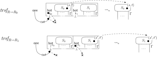
Figure 13: The Partial Function $\mathrm{trsf}$ on $\bot$-box Reduction.

Transformation of SIAM States.

For each $R_{i}$ to which $R$ reduces, we define a transformation on positions, as a partial function $\mathrm{trsf}_{R\rightsquigarrow R_{i}}:\mathtt{POS}_{R}\rightharpoonup\mathtt{POS}_{R_{i}}$. The key case is the case of $\bot$-box reduction, illustrated in Fig. 13; for each position outside the redex, we intend that $\mathrm{trsf}(\mathbf{p})$ is the identity. The other cases are as in Dal Lago et al. [2015].

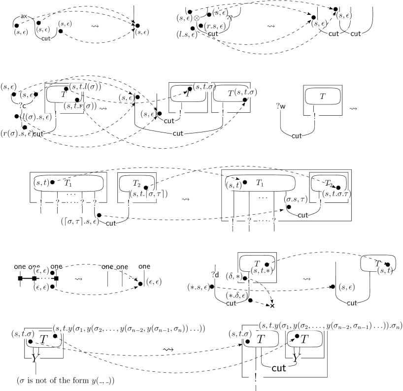
Figure 14: The Function $\mathrm{trsf}_{R\rightsquigarrow R^{\prime}}$.

The definition extends to the states of the SIAM point-wisely, in the obvious way.

From now on, we write $\mathrm{trsf}_{R_{i}}$ or sometimes simply $\mathrm{trsf}_{i}$ for $\mathrm{trsf}_{R\rightsquigarrow R_{i}}$.

Transformation of MSIAM States.

We now extend $\mathrm{trsf}_{R\rightsquigarrow R_{i}}$ to MSIAM  states. To do so smoothly, we define a subset $[\mathrm{trsf}_{R_{i}}]$ of $\mathcal{S}_{\mathbf{I}_{R}}$, which depends on the reduction rule. To work with such states simplify the proofs, and is always possible because of Sec. D.1.1.

• Case $\rightsquigarrow_{{\rm link}(n,j)}$. We define $[\mathrm{trsf}_{R_{i}}]$ as the set of the states in $\mathcal{S}_{\mathbf{I}_{R}}$ in which ${\tt ind}(\mathbf{p})=j$, where $\mathbf{p}$ is the position associated to the $\mathsf{one}$ node $n$.

• Case $\rightsquigarrow_{{\rm update}(s)}$. We define $[\mathrm{trsf}_{R_{i}}]$ as the set of the states in $\mathcal{S}_{\mathbf{I}_{R}}$ which “have crossed” the sync node $s$. We can easily characterize these states. Assume $\mathbf{p}_{1},\ldots,\mathbf{p}_{n}$ are the positions associated to the premises of $s$ (observe that each $\mathbf{p}_{i}$ belongs to $\mathtt{ONES}_{R}$). $[\mathrm{trsf}_{R_{i}}]$ is the set of the states $\mathbf{T}\in\mathcal{S}_{\mathbf{I}_{R}}$ such that $\{\mathbf{p}_{1},\ldots,\mathbf{p}_{n}\}\subseteq\mathrm{orig}(T)$ and $\{\mathbf{p}_{1},\ldots,\mathbf{p}_{n}\}\not\subseteq T$.

• Case $\rightsquigarrow_{{\rm test}(j)}$. We define $[\mathrm{trsf}_{R_{0}}]$ as the set of the states in $\mathcal{S}_{\mathbf{I}_{R}}$ which have a token on the left $\mathsf{bot}$ of the redex (the edge $e_{0}$ in the Fig. 13). We define $[\mathrm{trsf}_{R_{1}}]$ similarly.

• Otherwise: we define $[\mathrm{trsf}_{R_{i}}]=\mathcal{S}_{\mathbf{I}_{R}}$.

Definition 31 (Transformation Map).

1. $\mathrm{trsf}_{i}:[\mathrm{trsf}_{R_{i}}]\subset\mathcal{S}_{\mathbf{I}_{R}}\to\mathcal{S}_{R_{i}}$ maps the state $\mathbf{T}=[(T,{\tt ind},\mathbf{m})]$ into $[\mathrm{trsf}_{i}(T,{\tt ind},\mathbf{m})]$, with

   $$\mathrm{trsf}_{i}(T,{\tt ind},\mathbf{m})=(\mathrm{trsf}_{i}(T),{\tt ind},\mathbf{m}).$$

2. The definition extends linearly to distributions. Assume $\mu=\sum c_{k}\cdot\{\mathbf{T}_{k}\}$ and $\mathbf{T}_{k}\in[\mathrm{trsf}_{R_{i}}]$ for each $\mathbf{T}_{k}$, then

   $$\mathrm{trsf}_{R\rightsquigarrow R_{i}}(\mu):=\sum c_{k}\cdot\{\mathrm{trsf}_{R\rightsquigarrow R_{i}}(\mathbf{T}_{k})\}.$$

Fact 32.

If $\mathbf{T}\in[\mathrm{trsf}_{R_{i}}]$, with $\mathbf{T}\rightarrow\mu$ and $\mathbf{U}\in\mathit{SUPP}(\mu)$, then $\mathbf{U}\in[trsf_{R_{i}}]$.

Lemma 33 (Important Observation).

The construction given in D.1.1 leads each time to a distribution $\mu$, where each state in the support satisfies:

• $\mathbf{U}_{i}\in[\mathrm{trsf}_{R_{i}}].$

• $\mathrm{trsf}_{R_{i}}(\mathbf{U}_{i})=\mathbf{I}_{R_{i}}$.

D.1.3 Properties of the Reachable States

Let us analyze the set of states which is spanned by a run of the MSIAM. Given a $\bot$-box of $\mathbf{R}$, let $e_{0}$ be the conclusion of the left $\bot$ and $e_{1}$ be the conclusion of the right $\bot$. For any stacks $s,t$, we call the two stable positions $(e_{0},s,t)$ and $(e_{1},s,t)$ a $\bot$-pair. These two positions are mutually exclusive in a state, because $\mathrm{orig}(e_{0},s,t)=\mathrm{orig}(e_{1},s,t)$.

We say that two states $\mathbf{T},\mathbf{U}\in\mathcal{S}_{\mathbf{I}_{R}}$ are in conflict, written $\mathbf{T}\smile\mathbf{U}$, if $\mathbf{T}$ contains one of the two positions of a $\bot$-pair and $S$ the other. We observe that conflict is hereditary with respect to transitions, because stable positions are never deleted or modified by a transition. Let $\mathop{\uparrow}(\mathbf{T})=\{\mathbf{U}~{}|~{}\mathbf{T}\mathrel{\mathrel{\rightrightarrows}^{*}}\rho\,\land\,\mathbf{U}\in\mathit{SUPP}(\rho)\}$. The following properties are all immediate:

1. If $\mathbf{T}\smile\mathbf{T}^{\prime}$, $\mathbf{U}\in\mathop{\uparrow}(\mathbf{T})$, and $\mathbf{U}^{\prime}\in\mathop{\uparrow}(\mathbf{T}^{\prime})$, then $\mathbf{U}\smile\mathbf{U}^{\prime}$.

2. If $\mathbf{T}\rightarrow\mu$, either the transition is deterministic, or $\mathit{SUPP}(\mu)=\{\mathbf{U}_{0},\mathbf{U}_{1}\}$ with $\mathbf{U}_{0}\smile\mathbf{U}_{1}$.

3. If $\mathbf{I}\mathrel{\rightrightarrows}^{*}\mu$, then for each $\mathbf{T}\not=\mathbf{T}^{\prime}\in\mathit{SUPP}(\mu)$, $\mathbf{T}\smile\mathbf{T}^{\prime}$.

States in conflict are in particular disjoint. Therefore we can safely sum them:

Lemma 34.

Given a distribution of states $\mu\in\mathit{DST}(\mathcal{S}_{\mathbf{I}_{R}})$,

$$\mu\mathrel{\rightrightarrows}^{k}\sum_{\mathbf{T}\in\mathit{SUPP}(\mu)}\mu(\mathbf{T})\cdot\rho_{\mathbf{T}}\lx@proof@logical@and\forall\mathbf{T}_{i},\mathbf{T}_{j}\in\mathit{SUPP}(\mu).\mathbf{T}_{i}\smile\mathbf{T}_{j}~{}\{\mathbf{T}\mathrel{\rightrightarrows}^{k}\rho_{\mathbf{T}}\}_{\mathbf{T}\in\mathit{SUPP}(\mu)}\,.$$

As an immediate consequence, the following also hold:

$$\mathbf{U}\mathrel{\rightrightarrows}^{k+1}\sum_{\mathbf{T}\in\mathit{SUPP}(\mu)}\mu(\mathbf{T})\cdot\rho_{\mathbf{T}}\lx@proof@logical@and\mathbf{U}\rightarrow\mu\{\mathbf{T}\mathrel{\rightrightarrows}^{k}\rho_{\mathbf{T}}\}_{\mathbf{T}\in\mathit{SUPP}(\mu)}$$

$$\mathbf{U}\mathrel{\rightrightarrows}^{n+k}\sum_{\mathbf{T}\in\mathit{SUPP}(\mu)}\mu(\mathbf{T})\cdot\rho_{\mathbf{T}}\lx@proof@logical@and\mathbf{U}\mathrel{\rightrightarrows}^{n}\mu\{\mathbf{T}\mathrel{\rightrightarrows}^{k}\rho_{\mathbf{T}}\}_{\mathbf{T}\in\mathit{SUPP}(\mu)}$$

D.1.4 The Reachability Relation $\mathrel{\looparrowright}$

The reachability relation $\mathrel{\looparrowright}$ (defined in Sec. 2.1) is a useful tool in the study of the MSIAM.

A derivation of $a\mathrel{\looparrowright}\mu$ is inductively obtained by using the rules which define $\mathrel{\looparrowright}$.

In the case of the MSIAM  the relations $\mathrel{\looparrowright}$ and $\mathrel{\rightrightarrows}$ are equivalent with respect to normal forms.

Lemma 35.

If $\{\mathbf{T}\}\mathrel{\rightrightarrows}^{n}\xi$ then $\mathbf{T}\mathrel{\looparrowright}\xi$. Conversely, if $\mathbf{T}\mathrel{\looparrowright}\mu$ then there exists $\rho$ with $\{\mathbf{T}\}\mathrel{\rightrightarrows}^{*}\rho$ and such that $\mu^{\circ}\subseteq\rho^{\circ}$. ∎

Proof.

The former part is by induction on $n$. The latter is by structural induction (on the rules shown above). ∎

It is helpful to define also another auxiliary relation $\mathbf{T}\mathrel{{\mathrel{\looparrowright}^{\circ}}}\tau$ which holds if there exists $\mu$ satisfying $\mathrel{\looparrowright}\mu$ and $\tau\subseteq\mu^{\circ}$. This relation states that $\mathbf{T}$ reaches a set of terminal states. It is immediate that $\mathbf{T}\mathrel{{\mathrel{\looparrowright}^{\circ}}}\tau$ iff $\exists\rho$, $\mathbf{T}\mathrel{\rightrightarrows}^{*}\rho$ and $\tau\subseteq\rho^{\circ}$.

D.1.5 Properties of $\mathrm{trsf}$

We now study the action of $\mathrm{trsf}$ on transitions. We first look at how $\mathrm{trsf}$ maps initial/final/deadlock states.

Lemma 36.

1. If $\mathbf{I}_{\mathbf{R}}\in[\mathrm{trsf}_{R_{i}}]$, then $\mathrm{trsf}_{R_{i}}(\mathbf{I}_{\mathbf{R}})=\mathbf{I}_{\mathbf{R}_{i}}$ .

2. Assume $\mathbf{T}\in[\mathrm{trsf}_{R_{i}}]$ is a final/deadlock state of $\mathcal{M}_{R}$; then $\mathrm{trsf}_{R_{i}}(\mathbf{T})$ is a final/deadlock state of $\mathcal{M}_{R_{i}}$.

3. If $\tau=\tau^{\circ}$ (i.e. all states are terminal), and $\mathit{SUPP}(\tau)\subseteq[\mathrm{trsf}_{R_{i}}]$, then $\mathcal{T}(\tau)=\mathcal{T}(\mathrm{trsf}_{R_{i}}(\tau))$.

Lemma 37.

If $\mathbf{T}\smile\mathbf{T}^{\prime}$ and $\mathbf{T},\mathbf{T}^{\prime}\in[\mathrm{trsf}_{R_{i}}]$, then $\mathrm{trsf}_{R_{i}}(\mathbf{T})\smile\mathrm{trsf}_{R_{i}}(\mathbf{T}^{\prime})$

It is also important to understand the action of $\mathrm{trsf}$ on the number of stable tokens. We observe that the number of tokens, and stable tokens in particular, in any state $\mathbf{T}$ which is reached in a run of $\mathcal{M}_{R}$ is finite. We denote by $S(\mathbf{T})$ the number of stable tokens in $\mathbf{T}$. The following is immediate by analyzing the definition of transformation, and checking which tokens are deleted.

Fact 38 (stable tokens).

For any $\mathrm{trsf}_{R_{i}}$, $S(\mathbf{T})\geq S(\mathrm{trsf}_{R_{i}}(\mathbf{T}))$. Moreover, if the reduction $\rightsquigarrow$ is $d,y$ or $u_{i}$, then we also have that $S(\mathbf{T})>S(\mathrm{trsf}_{R_{i}}(\mathbf{T}))$.

D.2 Invariance

We prove the following result, from which invariance (Th. 27) follows.

Proposition 39 (Main Property).

Assume $\mathbf{R}\rightsquigarrow\sum_{i}{p_{i}}\cdot\{\mathbf{R}_{i}\}$. $\mathbf{I}_{\mathbf{R}}$ $q$-terminates if and only if $\mathbf{I}_{\mathbf{R}_{i}}$ $q_{i}$-terminates and $\sum(q_{i}\cdot p_{i})=q$.

Let us first sketch the ingredients of the proof. We need to work our way “back and forth” via Lemmas 42 and 43, because of the following facts.

• Unfortunately, for $\mathbf{I}_{\mathbf{R}}\mathrel{\rightrightarrows}^{*}\mu$ it is not true that $\mathrm{trsf}_{R_{i}}(\mathbf{I}_{\mathbf{R}})\mathrel{\rightrightarrows}^{*}\mathrm{trsf}_{R_{i}}(\mu)$. However we have that if $\mathbf{I}_{\mathbf{R}}\mathrel{\looparrowright}\mu$ in $\mathcal{M}_{R}$, then $\mathrm{trsf}_{R_{i}}(\mathbf{I}_{\mathbf{R}})\mathrel{\looparrowright}\mathrm{trsf}_{R_{i}}(\mu)$ (under natural conditions). This is made precise by Lemma 42.

• On the other side, the strength of the relation $\mathrel{\rightrightarrows}$ is that if $\mathbf{I}_{\mathbf{R}}\mathrel{\rightrightarrows}^{n}\mu$, then for any sequence of the same length $\mathbf{I}_{\mathbf{R}}\mathrel{\rightrightarrows}^{n}\rho$, we have that $\rho^{\circ}=\mu^{\circ}$. This is not the case for the relation $\mathrel{\looparrowright}$ which is not informative. The (slightly complex) construction which is given by Lemma 43 allows us to exploit the power of $\mathrel{\rightrightarrows}$.

We have everything in place to study the action of $\mathrm{trsf}$ on a run of the machine. What is the action of $\mathrm{trsf}$ on a transition? By checking the definition in Fig. 14 we observe that it may be the case that $\mathbf{T}\rightarrow\{\mathbf{U}\}$ and $\mathrm{trsf}_{R\rightsquigarrow R_{i}}(\mathbf{U})=\mathrm{trsf}_{R\rightsquigarrow R_{i}}(\mathbf{T})$. We say that such a transition collapses for $\mathrm{trsf}_{R\rightsquigarrow R_{i}}$. We observe some properties:

Lemma 40.

From a state of $\mathcal{M}_{R}$, we have at most a finite number of collapsing transitions.

Proof.

Since the reduction is surface, and since the type of any edge is finite, the set $\{(e,s,t)\,|\,e$ is an edge of the redex, $(e,s,t)$ is involved in a collapsing transition$\}$ is at most finite. Suppose there are infinitely many collapsing transitions from a state. Then there exist two or more tokens which have the same stacks involved in the sequence of transitions. They must have the same origin, and hence by injectivity they are in fact the “same” token visiting the redex twice or more. Therefore, by “backtracking” the transitions on that token, it again comes to the same edge in the redex with the same stack, hence we can go back infinitely many times. However this cannot happen in our MSIAM machine, since any token starts its journey from a position in $\mathtt{START}$ from which it cannot go back anymore, and transitions are bideterministic on each token. ∎

Fact 41.

Given a transition $\mathbf{T}\rightarrow\mu$, if $\mathbf{T}\in[\mathrm{trsf}_{R_{i}}]$, then either the transition collapses, or $\mathrm{trsf}_{R_{i}}(\mathbf{T})\rightarrow\mathrm{trsf}_{R_{i}}(\mu)$ is a transition of $\mathcal{M}_{R_{i}}$.

Lemma 42.

If $\mathbf{T}\in[\mathrm{trsf}_{R_{i}}]$ and $\mathbf{T}\mathrel{\looparrowright}\mu$ (in $\mathcal{M}_{R}$), then $\mathrm{trsf}_{R_{i}}(\mathbf{T})\mathrel{\looparrowright}\mathrm{trsf}_{R_{i}}(\mu)$ holds.

Proof.

We transform a derivation $\Pi$ of $\mathbf{T}\mathrel{\looparrowright}\mu$ in $\mathcal{M}_{R}$ into a derivation of $\mathrm{trsf}_{R_{i}}(\mathbf{T})\mathrel{\looparrowright}\mathrm{trsf}_{R_{i}}(\mu)$ in $\mathcal{M}_{R_{i}}$, by induction on the structure of the derivation.

• Case $\mathbf{T}{\mathrel{\looparrowright}}\{\mathbf{T}\}\quad\text{becomes}\quad\mathrm{trsf}_{R_{i}}\mathbf{T}{\mathrel{\looparrowright}}\{\mathrm{trsf}_{R_{i}}(\mathbf{T})\}$

• Case $\mathbf{T}{\mathrel{\looparrowright}}\sum p_{\mathbf{U}}\cdot\mu_{\mathbf{U}}\lx@proof@logical@and\mathbf{T}{\rightarrow}\sum p_{\mathbf{U}}\cdot\mathbf{U}\{\mathbf{U}{\mathrel{\looparrowright}}\mu_{\mathbf{U}}\dots\}$​​

  We examine the left premise, checking if it collapses:

  • If it does not collapse, $\mathrm{trsf}_{R_{i}}(\mathbf{T}){\rightarrow}\sum p_{\mathbf{U}}\cdot\mathrm{trsf}_{R_{i}}(\mathbf{U})$ is a transition of $\mathcal{M}_{R^{\prime}}$ and we have:

    $$\mathrm{trsf}_{R_{i}}(\mathbf{T}){\mathrel{\looparrowright}}\sum p_{\mathbf{U}}\cdot\mathrm{trsf}_{R_{i}}(\mu_{\mathbf{U}})\begin{array}[]{c}\mathrm{trsf}_{R_{i}}(\mathbf{T}){\rightarrow}\sum p_{\mathbf{U}}\cdot\mathrm{trsf}_{R_{i}}(\mathbf{U})\\ \{{\mathrm{trsf}_{R_{i}}(\mathbf{U})\mathrel{\looparrowright}\mathrm{trsf}_{R_{i}}(\mu_{\mathbf{U}})}\}\text{ by I.H.}\end{array}$$

  • If it collapses, we have $\mathbf{T}\rightarrow\{\mathbf{U}\}$, we also have $\mathrm{trsf}_{R_{i}}\mathbf{T}=\mathrm{trsf}_{R_{i}}(\mathbf{U})$,and the derivation $\Pi$ is of the form:

    $$\mathbf{T}{\mathrel{\looparrowright}}\mu\lx@proof@logical@and\mathbf{T}{\rightarrow}\{\mathbf{U}\}\mathbf{U}{\mathrel{\looparrowright}}\mu...$$

    By induction, $\mathrm{trsf}_{R_{i}}\mathbf{U}\mathrel{\looparrowright}\mathrm{trsf}_{R_{i}}(\mu)$, and therefore we conclude $\mathrm{trsf}_{R_{i}}\mathbf{T}\mathrel{\looparrowright}\mathrm{trsf}_{R_{i}}(\mu)$.

∎

Lemma 42, the construction shown in Appendix D.1.1, and Lemma 36, allow us to transfer termination from $\mathbf{I}_{\mathbf{R}}$ to $\mathbf{I}_{\mathbf{R}_{i}}$, and to prove one direction of Prop. 39. The other direction is more delicate.

Assume that $\mathbf{I}_{\mathbf{R}_{i}}$ $q_{i}$-terminates; this implies that for a certain $n$, whenever $\mathbf{I}_{\mathbf{R}_{i}}\mathrel{\rightrightarrows}^{n}\sigma$ then $\mathcal{T}(\sigma)\geq q$. The following Lemma builds such a sequence in a way that $\sigma=\mathrm{trsf}_{R_{i}}(\mu)$, with $\mu$ in $\mathcal{M}_{\mathbf{R}}$. This allows us to transfer the properties of termination of $\mathbf{I}_{\mathbf{R}_{i}}$ back to $\mathbf{I}_{\mathbf{R}}$, ultimately leading to the other direction of Prop. 39.

Lemma 43.

Assume $\mathbf{T}\in[\mathrm{trsf}_{R_{i}}]$ . For any $n$:

1. there exists $\mu$ such that $\mathbf{T}\mathrel{\looparrowright}\mu$ and $\mathrm{trsf}_{R_{i}}(\mathbf{T})\mathrel{\rightrightarrows}^{n}\mathrm{trsf}_{R_{i}}(\mu)$;

2. we can choose $\mu$ such that $\mathcal{T}(\mu)=\mathcal{T}(\mathrm{trsf}_{R_{i}}(\mu))$.

Proof.

1. We build $\mu$ and its derivation, by induction on $n$.

   1. • Assume $\mathbf{T}$ is terminal, then $\mathrm{trsf}_{R_{i}}(\mathbf{T})$ is terminal, and $\mathrm{trsf}_{R_{i}}(\mathbf{T})\mathrel{\rightrightarrows}\mathrm{trsf}_{R_{i}}(\mathbf{T})$.

      • Assume there is $\mu$ s.t. $\mathbf{T}\rightarrow\mu$ non-collapsing. We have $\mathrm{trsf}_{R_{i}}(\mathbf{T})\mathrel{\rightrightarrows}\mathrm{trsf}_{R_{i}}(\mu)$.

      • Assume that all transitions from $\mathbf{T}$ are collapsing. For such a reduction, we have that $\mathbf{T}\rightarrow\mathbf{T}^{\prime}$ and $\mathrm{trsf}_{R_{i}}(\mathbf{T})=\mathrm{trsf}_{R_{i}}(\mathbf{T}^{\prime})$. It is immediate to check that from any $\mathbf{T}\in\mathcal{S}_{\mathbf{I}_{R}}$ there is at most a finite number of consecutive collapsing transitions. We repeat our reasoning on $\mathbf{T}^{\prime}$ until we find $\mathbf{U}$ which is either terminal or has a non-collapsing transition $\mathbf{U}\rightarrow\mu$. The former case is immediate, the latter gives $\mathbf{U}\mathrel{\looparrowright}\mu$ and therefore $\mathbf{T}\mathrel{\looparrowright}\mu$ by transitivity, and $\mathrm{trsf}_{R_{i}}(\mathbf{T})=\mathrm{trsf}_{R_{i}}(\mathbf{U})\rightarrow\mathrm{trsf}_{R_{i}}(\mu)$, hence $\mathrm{trsf}_{R_{i}}(\mathbf{T})\mathrel{\rightrightarrows}\mathrm{trsf}_{R_{i}}(\mu)$.

   2. Assume we have built a derivation of $\mathbf{T}\mathrel{\looparrowright}\rho$ with

      $\mathrm{trsf}_{R_{i}}(\mathbf{T})\mathrel{\rightrightarrows}^{n-1}\mathrm{trsf}_{R_{i}}(\rho)$. We have that $\mathrm{trsf}_{R_{i}}(\rho)=\sum\rho(\mathbf{U})\cdot\mathrm{trsf}_{R_{i}}(\mathbf{U})$. For each $\mathbf{U}\in\mathit{SUPP}(\rho)$, we apply the base step, and obtain a derivation of $\mathbf{U}\mathrel{\looparrowright}\mu_{\mathbf{U}}$ with $\mathrm{trsf}_{R_{i}}(\mathbf{U})\mathrel{\rightrightarrows}\mathrm{trsf}_{R_{i}}(\mu_{\mathbf{U}})$. Putting things together, $\mathbf{T}\mathrel{\looparrowright}\sum\rho(\mathbf{U})\cdot\mu_{\mathbf{U}}$ and $\mathrm{trsf}_{R_{i}}(\mathbf{T})\mathrel{\rightrightarrows}^{n}\sum\rho(\mathbf{U})\cdot\mathrm{trsf}_{R_{i}}(\mu_{\mathbf{U}})$ by Lemma 34.

2. We now prove the second part of the claim. Let $\mathbf{T}\mathrel{\looparrowright}\mu$ be the result obtained at the previous point. Let $\{\mathbf{U}_{k}\}$ be the set of states in $\mathit{SUPP}(\mu)$ such that $\mathrm{trsf}_{R_{i}}(\mathbf{U}_{k})$ is terminal. This induces a partition of $\mu$, namely $\mu=\rho+\sum c_{k}\cdot\{\mathbf{U}_{k}\}$. It is immediate to check that each $\mathbf{U}_{k}\mathrel{\looparrowright}\{\mathbf{U}^{\prime}_{k}\}$ with $\mathbf{U}^{\prime}_{k}$ terminal and $\mathrm{trsf}_{R_{i}}(\mathbf{U}^{\prime}_{k})=\mathrm{trsf}_{R_{i}}(\mathbf{U}_{k})$. Observe also that $\rho$ does not contain any terminal state. Let $\nu=\sum c_{k}\cdot\{\mathbf{U}^{\prime}_{k}\}$. We have by transitivity $\mathbf{T}\mathrel{\looparrowright}(\rho+\nu)$, and $\mathrm{trsf}_{R_{i}}(\mathbf{T})\mathrel{\rightrightarrows}^{n}\mathrm{trsf}_{R_{i}}(\rho+\nu)$ (because $\mathrm{trsf}_{R_{i}}(\rho+\nu)=\mathrm{trsf}_{R_{i}}(\mu)$). We have $\mathcal{T}(\mathrm{trsf}_{R_{i}}(\rho+\nu))=\mathcal{T}(\mathrm{trsf}_{R_{i}}(\nu))=\sum c_{k}$ because $\mathrm{trsf}_{R_{i}}(\nu)=\sum c_{k}\cdot\mathrm{trsf}_{R_{i}}(\mathbf{U}^{\prime}_{k})$. We conclude by observing that $\mathcal{T}(\rho+\nu)=\mathcal{T}(\nu)=\sum c_{k}$.

∎

Summing up, we now have all the elements to prove Prop. 39.

Proof.

(Prop. 39)

$\Rightarrow$. Follows from Prop. 42, by using the construction in Sec. D.1.1, Lemma 36, and linearity of $\mathrm{trsf}$.

Assume $\mathbf{I}_{R}\mathrel{\rightrightarrows}^{*}\mu$, with $\mu^{\circ}$ not empty, and that the machine starts as described in Sec. D.1.1 (in case $\rightsquigarrow$ is link, update or test). We observe that every state $\mathbf{T}\in\mathit{SUPP}(\mu)$ is contained in $[\mathrm{trsf}_{i}]$ for some $i$. We can then prove that for each $i$ there exists $\mu_{i}\in\mathit{DST}(\mathcal{S}_{\mathbf{I}_{R}})$ such that $\mathbf{I}_{R_{i}}\mathrel{\looparrowright}\mathrm{trsf}_{R_{i}}(\mu_{i})$, and such that $\nu=\sum_{i}p_{i}\cdot\mu_{i}$.

$\Leftarrow$. Follows from Lemma 43. We examine the only non-straightforward case. Assume $\mathbf{R}\rightsquigarrow_{\mathrm{test(i,\mathbf{m})}}\{\mathbf{R}_{0}^{p_{0}},\mathbf{R}_{1}^{p_{1}}\}$. We choose a run of the machine which starts as described in Sec. D.1.1; we have that $\mathbf{I}_{\mathbf{R}}\mathrel{\looparrowright}\sum p_{i}\cdot\{\mathbf{T}_{i}\}$, with $\mathrm{trsf}_{R_{i}}(\mathbf{T}_{i})=\mathbf{I}_{\mathbf{R}_{i}}$ by Lemma 33. By hypothesis, $\mathbf{I}_{\mathbf{R}_{i}}$ terminates with probability at least $q_{i}$; assume it does so in $n$ steps. By using Lemma 43, we build a derivation $\mathbf{T}_{i}\mathrel{\looparrowright}\mu_{i}$ such that $\mathrm{trsf}_{R_{i}}(\mathbf{T}_{i})\mathrel{\rightrightarrows}^{n}\mathrm{trsf}_{R_{i}}(\mu_{i})$ and $\mathcal{T}(\mu_{i})=\mathcal{T}(\mathrm{trsf}_{R_{i}}(\mu_{i}))$. By Th. 11, $\mathcal{T}(\mathrm{trsf}_{R_{i}}(\mu_{i}))\geq q_{i}$.

Putting all together, we have that $\mathbf{I}_{\mathbf{R}}\mathrel{\looparrowright}\sum p_{i}\cdot\mu_{i}$, and $\mathbf{I}_{\mathbf{R}}$ terminates with probability at least $\sum p_{i}\cdot q_{i}$. ∎

D.3 MSIAM Adequacy and Deadlock-Freeness: The Interplay of Nets and Machines

We are now able to establish adequacy (Th. 28) and deadlock-freeness (Th. 26). Both are direct consequence of Prop. 45 below, which in turn follows form Prop. 39 and the following Fact, by finely exploiting the interplay between nets and machine.

Fact 44.

Let $R$ be a net of conclusion $\mathsf{1}$ and such that no reduction is possible. By Th. 22, $R$ has no cuts, and is therefore simply a $\mathsf{one}$ node. On such a simple net, $\mathcal{M}_{R}$ can only terminate in a final state: no deadlock is possible.

Proposition 45 (Mutual Termination).

Let $\mathbf{R}$ be a net of conclusion $\mathsf{1}$. The following are equivalent:

• $\mathbf{I}_{\mathbf{R}}$ q-terminates;

• $\mathbf{R}$ q-terminates;

Moreover

1. if $\mathbf{I}_{\mathbf{R}}\mathrel{\looparrowright}\mu$ and $\mathbf{T}\in\mathit{SUPP}(\mu)$ is terminal, then $\mathbf{T}$ is a final state.

Proof.

(1. $\Rightarrow$ 2.) and 3. We prove that

if $\mathbf{I}_{\mathbf{R}}\mathrel{{\mathrel{\looparrowright}^{\circ}}}\tau$, then $\begin{array}[]{l}\mbox{(*) $\mathbf{R}$ terminates with probability at least $\mathcal{T}(\tau)$,}\\ \mbox{(**) all states in $\mathit{SUPP}(\tau)$ are final.}\end{array}$

The proof is by double induction on the lexicographically ordered pair $(S(\tau),W(\mathbf{R}))$, where $W(\mathbf{R})$ is the weight of the cuts at the surface of $\mathbf{R}$, and $S(\tau)=\sum_{\mathbf{T}\in\mathit{SUPP}(\tau)}S(\mathbf{T})$ with $S(\mathbf{T})$ the number of stable tokens in $\mathbf{T}$ (Fact38). Both parameters are finite.

We will largely use the following fact (immediate consequence of the definition of $\mathrel{{\mathrel{\looparrowright}^{\circ}}}$ and of results we have already proved): if $\mathbf{T}\mathrel{{\mathrel{\looparrowright}^{\circ}}}\tau$ in $\mathcal{M}_{\mathbf{R}}$ and $\mathbf{T}\in[\mathrm{trsf}_{i}]$, then $\mathrm{trsf}_{i}(\mathbf{T})\mathrel{{\mathrel{\looparrowright}^{\circ}}}\mathrm{trsf}_{i}(\tau)$.

• If $\mathbf{R}$ has no reduction step, then $\mathcal{T}(\mathbf{R})=1$, which trivially proves (*); (**) holds by Fact 44.

• Assume $\mathbf{R}\rightsquigarrow_{\not{\rm test}(i,\mathbf{m})}\mathbf{R}^{\prime}$ (observe that this is a deterministic reduction). We have that $\mathbf{I}_{\mathbf{R}^{\prime}}\mathrel{{\mathrel{\looparrowright}^{\circ}}}\mathrm{trsf}(\tau)$, and $\mathcal{T}(\mathrm{trsf}(\tau))=\mathcal{T}(\tau)$. By Fact 38, $S(\mathrm{trsf}(\tau))\leq S(\tau)$. If $\mathbf{R}\rightsquigarrow_{d}\mathbf{R}^{\prime}$, then $S(\mathrm{trsf}(\tau))<S(\tau)$. Otherwise $S(\mathrm{trsf}(\tau))=S(\tau)$ but $W(\mathbf{R}^{\prime})<W(\mathbf{R})$ because the step reduces a cut at the surface, and does not open any box. Hence by induction, $\mathbf{R}^{\prime}$ terminates with probability at least $\mathcal{T}(\mathrm{trsf}(\tau))=\mathcal{T}(\tau)$ (and therefore so does $\mathbf{R}$) and all states in $\mathrm{trsf}(\tau)$ are final, from which (**) holds by Lemma 36.2.

• Assume $\mathbf{R}\mathrel{\rightsquigarrow_{{\rm test}(i,\mathbf{m})}}\sum p_{i}\cdot\{\mathbf{R}_{i}\}$. From $\mathbf{I}_{\mathbf{R}}\mathrel{{\mathrel{\looparrowright}^{\circ}}}\tau$, by Lemma 35 we have that there is $\rho$ satisfying $\mathbf{I}_{\mathbf{R}}\mathrel{\rightrightarrows}^{*}\rho$ and $\tau\subseteq\rho^{\circ}$. Using the construction in Sec. D.1.1, we have $\mathbf{I}_{\mathbf{R}}\mathrel{\rightrightarrows}^{*}\sum p_{i}\cdot\{\mathbf{T}_{i}\}$, which induces a partition of $\tau$ in $\tau=p_{0}\cdot\tau_{0}+p_{1}\cdot\tau_{1}$ with $\mathbf{T}_{i}\mathrel{{\mathrel{\looparrowright}^{\circ}}}\tau_{i}$ for each $i$. We have that $S(\tau_{i})<S(\tau)$, and that $\mathbf{I}_{\mathbf{R}_{i}}\mathrel{{\mathrel{\looparrowright}^{\circ}}}\mathrm{trsf}_{i}(\tau_{i})$, because $\mathrm{trsf}_{i}(\mathbf{T}_{i})$ is defined and therefore $\mathrm{trsf}_{i}(\mathbf{U})$ is defined for each state $\mathbf{U}\in\tau_{i}$. By Fact 38, $S(\mathrm{trsf}_{i}(\tau_{i}))\leq S(\tau_{i})<S(\tau)$, thus by induction $\mathbf{R}_{i}$ terminates with probability at least $\mathcal{T}(\mathrm{trsf}_{i}(\tau_{i}))$, and all states in $\mathit{SUPP}(\mathrm{trsf}_{i}(\tau_{i}))$ are final. Therefore, $\mathbf{R}$ terminates with probability at least $\sum p_{i}\cdot\mathcal{T}(\mathrm{trsf}_{i}(\tau_{i}))=\sum p_{i}\cdot\mathcal{T}(\tau_{i})=\mathcal{T}(\tau)$ by Lemma 36.3, and all states in $\mathit{SUPP}(\tau)$ are final by Lemma 36.2.

2. $\Rightarrow$ 1. By hypothesis, $\mathbf{R}\mathrel{\rightrightarrows}^{n}\rho$ with $\mathcal{T}(\rho)\geq q$. We prove the implication by induction on $n$.

Case $n=0$. The implication is true by Fact 44.

Case $n>0$. Assume $\mathbf{R}\rightsquigarrow\sum p_{i}\cdot\mathbf{R}_{i}$. By hypothesis, each $\mathbf{R}_{i}$ terminates with probability at least $q_{i}$ (with $\sum p_{i}\cdot q_{i}=q$). By induction, each $\mathbf{I}_{\mathbf{R}_{i}}$ $q_{i}$-terminates, and therefore (Prop. 39) $\mathbf{I}_{\mathbf{R}}$ $q$-terminates. ∎

D.4 MSIAM: Full development of Fig. 10

Here we fully develop what was sketched as description of the MSIAM execution presented in Fig. 10.

In the first panel (A), no box are yet opened: only two tokens are generated: the dereliction node emits token (a), in state $(*.\delta,\epsilon)^{\downarrow}$, while the $\mathsf{one}$-node emits token (b), in state $(\epsilon,\epsilon)^{\downarrow}$, and attached to a fresh address of the memory. Eventually token (a) reaches the entrance of the $Y$-box and opens a copy: its state is now $(\delta,*.\epsilon)^{\leftrightarrow}$. Token (b) also flows down: it first reaches the $\mathsf{H}$-sync node, crosses it while updating the memory, crosses the $\otimes$-node and gets the new state $(l.\epsilon,\epsilon)^{\downarrow}$. It continues through $\mathsf{?d}$ with new state $(*.l.\epsilon,\epsilon)$, reaches the $Y$-entrance: its copy ID is $*.\epsilon$, and it has been opened by token (a), it can carry onto the left branch with new state $(l.\epsilon,*.\epsilon)$. It arrives at the $\parr$-node and follow the left branch with state $(\epsilon,*.\epsilon)$: it now hits a bot-box.

The test-action of the memory is called, and a probabilistic distribution of states is generated where the left and the right-side of the $\bot$-box are probabilistically opened: the corresponding sequences of operations are represented in Panel (B₀) for the left side, and Panel (B₁) for the right side.

In Panel (B₀): the left-side of the bot-box is opened and its $\mathsf{one}$-node emits token (c), in state $(\epsilon,*.\epsilon)$: note how the box stack of this newly-created token is the one of the copy of the $Y$-box it sits in. In any case, the token also comes equipped with a fresh address from the memory, and carries downward. When it reaches the entrance of the $Y$-box, coming from the left it exits and eventually reaches the conclusion of the net. Note how we end up with a normal form: token (b) and (a) are stable at doors of boxes.

In Panel (B₁): the right-side of the bot-box is opened and its $\mathsf{one}$-node emits a token, that we can also call (c), also in state $(\epsilon,*.\epsilon)$. The $\mathsf{?d}$-node emits token (d) in state $(*.\delta,*.\epsilon)$: this token flows down and gets to the entrance of the $Y$-box: it stops there in state $(\delta,y(*,*).\epsilon)$ and opens a new copy of the $Y$-box. Token (c) goes down, arrives at the $Y$-entrance and enters this new copy (of ID $y(*,*)$). It hits the corresponding copy of the $\bot$-box, and the test-action of the memory spawns a new probabilistic distributions.

We focus on panel (C₁₀) on the case of the opening of the left-side of the $\bot$-box: there, a new token (e) is generated (with a fresh address attached to it) and goes down. It will exit the copy of ID $y(*,*)$, enter the first copy, goes over the axiom node, and eventually exits from this first $Y$-box-copy. It is now at level 0, and goes to the conclusion of the net. The machine is in normal form.

Appendix E $\mathsf{PCF}^{\mathsf{LL}}$: Adequacy

The translation of $\mathsf{PCF}_{\mathsf{AM}}$ closures into program nets is given in Fig. 15 and 16. There, we assume that the translation is with respect to the fixed pair $({\tt ind},\mathbf{m})$. The partial map ${\tt ind}_{R_{M}}$ is depicted with a dotted line, and corresponds exactly to the parameter to the map ${(-)}^{\dagger}_{{\tt ind},\mathbf{m}}$.

Figure 15: Translation of $\mathsf{PCF}^{\mathsf{LL}}$ into Nets.

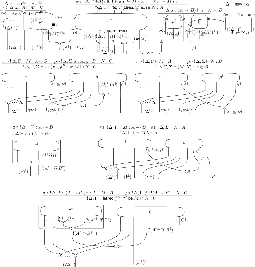
Figure 16: Translation of $\mathsf{PCF}^{\mathsf{LL}}$ into Nets.

With this definition, the well-typed closure $y_{1}:A_{1},\ldots,y_{m}:A_{m}\vdash(M,{\tt ind},\mathbf{m}):B$ can now simply be mapped to the program net ${M}^{\dagger}_{{\tt ind},\mathbf{m}}$.

We prove here the adequacy theorem (Th. 29).

Th. 29 (Recall).  Let $\vdash\textbf{M}:\alpha$, then $\textbf{M}\,{\Downarrow_{p}}$ if and only if ${\textbf{M}}^{\dagger}{\Downarrow_{p}}$.

Before proving the theorem, we first establish a few technical lemmas which analyze the properties of the translation ${(-)}^{\dagger}$.

Lemma 46.

Assume that $\textbf{M}=(M,{\tt ind},\mathbf{m})$ is $\mathsf{PCF}_{\mathsf{AM}}$ closure that $\vdash\textbf{M}:\alpha$, and $\mu$ a distribution of such closures. We have:

1. M is a normal form if and only if ${\textbf{M}}^{\dagger}$ is a normal form.

2. $\mathcal{T}(\mu)=\mathcal{T}({\mu}^{\dagger})$.∎

Lemma 47.

Under the hypotheses of Lemma 46:

1. if $\textbf{M}\to\mu$ then ${\textbf{M}}^{\dagger}\mathrel{\rightrightarrows}^{k}{\mu}^{\dagger}$, with $k\geq 1$.

2. if $\mu\mathrel{\rightrightarrows}^{*}\nu$ then ${\mu}^{\dagger}\mathrel{\rightrightarrows}^{*}{\nu}^{\dagger}$.∎

Corollary 48.

Under the hypotheses of Lemma 46:

1. If ${\textbf{M}}^{\dagger}\rightsquigarrow\rho$, then there is $\mu$ s.t. $\textbf{M}\to\mu$ with ${\textbf{M}}^{\dagger}\not={\mu}^{\dagger}$.

2. If ${\textbf{M}}^{\dagger}\mathrel{\rightrightarrows}^{k}\rho$, then there is $\mu$ s.t. $\textbf{M}\mathrel{\rightrightarrows}^{*}\mu$ and ${\textbf{M}}^{\dagger}\mathrel{\rightrightarrows}^{m}{\mu}^{\dagger}$, with $m\geq k$.

Proof.

(1.) Immediate consequence of Lemma 46 and 47 (2.) By induction. ∎

We are now ready to prove Th. 29.

Proof of Th. 29.

Assume $\textbf{M}\Downarrow_{p_{\it term}}$ and ${\textbf{M}}^{\dagger}\Downarrow_{p_{\it net}}$; we want to prove that $p_{\it term}=p_{\it net}$.

$\mathbf{p_{term}\leq p_{net}}$. It follows from the following. Assume $\textbf{M}\mathrel{\rightrightarrows}^{*}\mu$ with $\mathcal{T}(\mu)=q$, then ${\textbf{M}}^{\dagger}\mathrel{\rightrightarrows}^{*}{\mu}^{\dagger}$ (by Lemma 47.2) and $\mathcal{T}({\mu}^{\dagger})=q$ (by Lemma 46.2).

$\mathbf{p_{term}\geq p_{net}}$. We prove that if ${\textbf{M}}^{\dagger}\mathrel{\rightrightarrows}^{*}\rho$ then it exists $\mu$ with $\textbf{M}\mathrel{\rightrightarrows}^{*}\mu$ and $\mathcal{T}(\mu)\geq\mathcal{T}(\rho)$. Assume ${\textbf{M}}^{\dagger}\mathrel{\rightrightarrows}^{k}\rho$. By Corollary 48, $\textbf{M}\mathrel{\rightrightarrows}^{*}\mu$ and ${\textbf{M}}^{\dagger}\mathrel{\rightrightarrows}^{m}{\mu}^{\dagger}$, with $m\geq k$. By Uniqueness of Normal Forms (Th. 11.1) we have that $\mathcal{T}({\mu}^{\dagger})\geq\mathcal{T}(\rho)$. By Lemma 46, $\mathcal{T}(\mu)=\mathcal{T}({\mu}^{\dagger})$, from which we deduce the statement. ∎

References

- de Leeuw et al. [1955] K. de Leeuw, E. F. Moore, et al. Computability by probabilistic machine. In Automata Studies. Princeton U. Press, 1955.
- Nielsen and Chuang [2011] M. A. Nielsen and I. L. Chuang. Quantum Computation and Quantum Information: 10th Anniversary Edition. Cambridge University Press, 10th edition, 2011.
- Miller [1975] G. L. Miller. Riemann’s hypothesis and tests for primality. In STOC, pages 234–239, 1975.
- Rabin [1980] M. O. Rabin. Probabilistic algorithm for testing primality. Journal of Number Theory, 12(1):128 – 138, 1980.
- Shor [1994] P. W. Shor. Algorithms for quantum computation: Discrete logarithms and factoring. In SFCS, pages 124–134, 1994.
- Whitfield et al. [2011] J. D. Whitfield, J. Biamonte, and A. Aspuru-Guzik. Simulation of electronic structure hamiltonians using quantum computers. Molecular Physics, 109(5):735–750, 2011.
- Harrow et al. [2009] A. W. Harrow, A. Hassidim, and S. Lloyd. Quantum algorithm for linear systems of equations. Phys. Rev. Lett., 103:150502, Oct 2009.
- Kozen [1981] D. Kozen. Semantics of probabilistic programs. Journal of Computer System Sciences, 22:328–350, 1981.
- Plotkin [1982] G. Plotkin. Probabilistic powerdomains. In CAAP, 1982.
- Gay [2006] S. J. Gay. Quantum programming languages: survey and bibliography. Mathematical Structures in Computer Science, 16(4):581–600, 2006.
- Selinger and Valiron [2006] P. Selinger and B. Valiron. A lambda calculus for quantum computation with classical control. Math. Struct. in Comp. Sc., 16(3):527–552, 2006.
- Green et al. [2013] A. S. Green, P. LeFanu Lumsdaine, et al. Quipper: A scalable quantum programming language. In PLDI, pages 333–342, 2013.
- Pagani et al. [2014] M. Pagani, P. Selinger, and B. Valiron. Applying quantitative semantics to higher-order quantum computing. In POPL, pages 647–658, 2014.
- Girard [1987] J.-Y. Girard. Linear logic. Theor. Comput. Sci., 50:1–102, 1987.
- Abramsky et al. [2000] S. Abramsky, R. Jagadeesan, and P. Malacaria. Full abstraction for PCF. Inf. Comput., 163(2):409–470, 2000.
- Hyland and Ong [2000] J. M. E. Hyland and C.-H. Luke Ong. On full abstraction for PCF: I, II, and III. Inf. Comput., 163(2):285–408, 2000.
- Girard [1989] J.-Y. Girard. Geometry of interaction I: Interpretation of system F. Logic Colloquium 88, 1989.
- Lafont [1988] Y. Lafont. Logiques, catégories et machines. PhD thesis, Université Paris 7, 1988.
- Melliès [2009] P.-A. Melliès. Categorical semantics of linear logic. Panoramas et Synthèses, 12, 2009.
- Selinger [2004] P. Selinger. Towards a quantum programming language. Math. Struct. in Comp. Sc., 14(4):527–586, 2004.
- Hasuo and Hoshino [2011] I. Hasuo and N. Hoshino. Semantics of higher-order quantum computation via geometry of interaction. In LICS, pages 237–246, 2011.
- Delbecque [2009] Y. Delbecque. Quantum games as quantum types. PhD thesis, McGill University, 2009.
- Delbecque and Panangaden [2008] Y. Delbecque and P. Panangaden. Game semantics for quantum stores. Electr. Notes Theor. Comput. Sci., 218:153–170, 2008.
- Dal Lago and Zorzi [2014] U. Dal Lago and M. Zorzi. Wave-style token machines and quantum lambda calculi. In LINEARITY, pages 64–78, 2014.
- Dal Lago et al. [2014] U. Dal Lago, C. Faggian, I. Hasuo, and A. Yoshimizu. The geometry of synchronization. In CSL-LICS, pages 35:1–35:10, 2014.
- Danos and Regnier [1999] V. Danos and L. Regnier. Reversible, irreversible and optimal lambda-machines. Theor. Comput. Sci., 227(1-2):79–97, 1999.
- Mackie [1995] Ian Mackie. The geometry of interaction machine. In POPL, pages 198–208, 1995.
- Dal Lago et al. [2015] U. Dal Lago, C. Faggian, B. Valiron, and A. Yoshimizu. Parallelism and synchronization in an infinitary context. In LICS, pages 559–572, 2015.
- Dal Lago et al. [2017] U. Dal Lago, C. Faggian, B. Valiron, and A. Yoshimizu. The geometry of parallelism: Classical, probabilistic, and quantum effects. In POPL, 2017.
- Mackie [1994] I. Mackie. Applications of the Geometry of Interaction to language implementation. Phd thesis, University of London, 1994.
- Ghica et al. [2011] D. R. Ghica, A. Smith, and S. Singh. Geometry of synthesis IV. In ICFP, pages 221–233, 2011.
- Abramsky et al. [2002] S. Abramsky, E. Haghverdi, and P. J. Scott. Geometry of interaction and linear combinatory algebras. Math. Struct. in Comp. Sc., 12(5):625–665, 2002.
- Ehrhard et al. [2014] T. Ehrhard, C. Tasson, and M. Pagani. Probabilistic coherence spaces are fully abstract for probabilistic PCF. In POPL, pages 309–320, 2014.
- Danos and Harmer [2002] V. Danos and R. Harmer. Probabilistic game semantics. ACM Trans. Comput. Log., 3(3):359–382, 2002.
- Hoshino et al. [2014] N. Hoshino, K. Muroya, and I. Hasuo. Memoryful geometry of interaction. In CSL-LICS, page 52, 2014.
- Staton [2015] S. Staton. Algebraic effects, linearity, and quantum programming languages. In POPL, pages 395–406, 2015.
- Coecke et al. [2012] B. Coecke, R. Duncan, A. Kissinger, and Q. Wang. Strong complementarity and non-locality in categorical quantum mechanics. In LICS, pages 245–254, 2012.
- Ghica [2007] D. R. Ghica. Geometry of synthesis: a structured approach to VLSI design. In POPL, pages 363–375, 2007.
- Muroya et al. [2016] K. Muroya, N. Hoshino, and I. Hasuo. Memoryful geometry of interaction II: recursion and adequacy. In POPL, pages 748–760, 2016.
- Bezem and Klop [2003] M. Bezem and J. W. Klop. Term Rewriting Systems, volume 55 of Cambridge Tracts in Theoretical Computer Science, chapter Abstract Reduction Systems. Cambridge University Press, 2003.
- Pitts [2013] A. Pitts. Nominal Sets: Names and Symmetry in Computer Science. Cambridge University Press, 2013.
- Dal Lago et al. [2016] U. Dal Lago, C. Faggian, B. Valiron, and A. Yoshimizu. The geometry of parallelism: Classical, probabilistic, and quantum effects (long version). Available at https://arxiv.org/abs/1610.09629, 2016.