Maximum Rate of Growth of Enstrophy in Solutions of the Fractional Burgers Equation

Abstract

This investigation is a part of a research program aiming to characterize the extreme behavior possible in hydrodynamic models by analyzing the maximum growth of certain fundamental quantities. We consider here the rate of growth of the classical and fractional enstrophy in the fractional Burgers equation in the subcritical and supercritical regimes. Since solutions to this equation exhibit, respectively, globally well-posed behavior and finite-time blow-up in these two regimes, this makes it a useful model to study the maximum instantaneous growth of enstrophy possible in these two distinct situations. First, we obtain estimates on the rates of growth and then show that these estimates are sharp up to numerical prefactors. This is done by numerically solving suitably defined constrained maximization problems and then demonstrating that for different values of the fractional dissipation exponent the obtained maximizers saturate the upper bounds in the estimates as the enstrophy increases. We conclude that the power-law dependence of the enstrophy rate of growth on the fractional dissipation exponent has the same global form in the subcritical, critical and parts of the supercritical regime. This indicates that the maximum enstrophy rate of growth changes smoothly as global well-posedness is lost when the fractional dissipation exponent attains supercritical values. In addition, nontrivial behavior is revealed for the maximum rate of growth of the fractional enstrophy obtained for small values of the fractional dissipation exponents. We also characterize the structure of the maximizers in different cases.

Keywords: Fractional Burgers equation; extreme behavior; enstrophy growth; numerical optimization; gradient methods

AMS subject classifications: 35B45, 35Q35, 65K10

1 Introduction

One of the key questions studied in the mathematical analysis of evolutionary partial differential equations (PDEs) is the existence of solutions, both locally and globally in time. The motivation is that, in order to justify the application of different PDEs as models of natural phenomena, these equations must be guaranteed to possess meaningful solutions for physically relevant data. In addition, characterization of the extreme behavior which can be exhibited by the solutions of different PDEs is also relevant for our understanding of the worst-case scenarios which can be realized in the actual physical systems these PDEs describe. These two types of questions can be investigated by studying the time evolution of suitable Sobolev norms of the solutions. In particular, should a given Sobolev norm of the solution become unbounded at a certain time due to a spontaneous formation of a singularity, this will signal that the solution is no longer defined in that Sobolev space; this loss of regularity is referred to as “blow-up”.

An example of an evolutionary PDE model with widespread applications whose global-in-time existence remains an open problem is the three-dimensional (3D) Navier-Stokes system describing the motion of viscous incompressible fluids. Questions of existence of solutions to this system are usually studied for problems defined on unbounded or periodic domains $\Omega$, i.e., $\Omega={\mathbb{R}}^{d}$ or $\Omega=\SS^{d}$, where $d=2,3$. Unlike the two-dimensional (2D) problem where smooth solutions are known to exist globally in time [1], in 3D existence of such solutions has been established for short times only [2]. Establishing global existence of smooth solutions in 3D is one of the key open questions in mathematical fluid mechanics and, in fact, its importance for mathematics in general has been recognized by the Clay Mathematics Institute as one of its “millennium problems” [3]. Suitable weak solutions were shown to exist in 3D for arbitrarily long times [4], however, such solutions may not be regular in addition to being nonunique. Similar questions also remain open for the 3D Euler equation [5]. While many angles of attack on this problem have been pursued in mathematical analysis, one research direction which has received a lot of attention focuses on the evolution of the enstrophy ${\mathcal{E}}({\bf u})$ which for an incompressible velocity field ${\bf u}(t,\cdot)\;:\;\Omega\rightarrow{\mathbb{R}}^{d}$ at a given time $t$ is defined as ${\mathcal{E}}({\bf u}(t)):=(1/2)\int_{\Omega}|\boldsymbol{\nabla}\times{\bf u}(t,{\bf x})|^{2}\,d\Omega=(1/2)\|\boldsymbol{\nabla}{\bf u}(t,\cdot)\|_{L^{2}(\Omega)}^{2}$, where “$:=$” means “equals to by definition”, i.e., it is proportional to the square of the $L^{2}$ norm of the vorticity $\boldsymbol{\nabla}\times{\bf u}$. The reason why this quantity is interesting in the context of the 3D Navier-Stokes equation is due to a conditional regularity result proved by Foias and Temam [6] who showed that the solution remains smooth (i.e., stays in a suitable Gevrey regularity class) as long as the enstrophy remains bounded, i.e., for all $t$ such that ${\mathcal{E}}({\bf u}(t))<\infty$. In other words, a loss of regularity must be manifested by the enstrophy becoming infinite. While there exist many different conditional regularity results, this one is particularly useful from the computational point of view as it involves an easy to evaluate quadratic quantity. Analogous conditional regularity results, although involving other norms of vorticity, were also derived for the 3D Euler equation (e.g., the celebrated Beale-Kato-Majda (BKM) criterion [7]).

In order to assess whether or not the enstrophy can blow up in finite time one needs to study its instantaneous rate of growth $d{\mathcal{E}}/dt$ which can be estimated as [2]

$$\frac{d{\mathcal{E}}}{dt}<C\,{\mathcal{E}}^{3},$$ (1)

for some $C>0$ (hereafter $C$ will denote a generic positive constant whose actual value may vary between different estimates). It was shown in [8, 9], see also [10], that this estimate is in fact sharp, in the sense that, for each given enstrophy $\bar{{\mathcal{E}}}>0$ there exists an incompressible velocity field $\widetilde{\mathbf{u}}_{\bar{{\mathcal{E}}}}$ with ${\mathcal{E}}(\widetilde{\mathbf{u}}_{\bar{{\mathcal{E}}}})=\bar{{\mathcal{E}}}$, such that $d{\mathcal{E}}(\widetilde{\mathbf{u}}_{\bar{{\mathcal{E}}}})/dt\sim\bar{{\mathcal{E}}}^{3}$ as $\bar{{\mathcal{E}}}\rightarrow+\infty$. The fields $\widetilde{\mathbf{u}}_{\bar{{\mathcal{E}}}}$ were found by numerically solving a family of variational maximization problems for different values of $\bar{{\mathcal{E}}}$ (details of this approach will be discussed further below). However, the corresponding finite-time estimate obtained by integrating (1) in time takes the form

$${{\mathcal{E}}({\bf u}(t))\leq\frac{\bar{{\mathcal{E}}}}{\sqrt{1-\frac{C}{2}\,\bar{{\mathcal{E}}}^{2}\,t}}},\quad t\geq 0,$$ (2)

and it is clear that based on this estimate alone it is not possible to ensure a prior boundedness of enstrophy in time. Thus, the question of finite-time blow-up may be recast in terms of whether or not it is possible to find initial data ${\bf u}_{0}$ such that the corresponding flow evolution saturates the right-hand side of (2). We emphasize that for this to happen the rate of growth of enstrophy given in (1) would need to be sustained over a finite window of time, rather than just instantaneously, a behavior which has not been observed so far [10] (in fact, a singularity may arise in finite time even with enstrophy growth occurring at a slower sustained rate of $d{\mathcal{E}}/dt\sim{\mathcal{E}}^{\gamma}$ where $\gamma>2$ [10]).

The question of the maximum enstrophy growth has been tackled in computational studies, usually using initial data chosen in an ad-hoc manner, producing no evidence of a finite-time blow-up in the 3D Navier-Stokes system [11, 12, 13, 14, 15]. However, for the 3D Euler system the situation is different and the latest computations reported in [16, 17] indicate the possibility of a finite-time blow-up. A new direction in the computational studies of extreme behavior in fluid flow models relies on the use of variational optimization approaches to systematically search for the most singular initial data. This research program, initiated in [8, 9], aims to probe the sharpness, or realizability, of certain fundamental estimates analogous to (1) and (2) and defined for various hydrodynamic models such as the one-dimensional (1D) viscous Burgers equation and the 2D/3D Navier-Stokes system. Since the 1D viscous Burgers equation and the 2D Navier-Stokes system are both known to be globally well-posed in the classical sense [1], there is no question about the finite-time blow-up in these problems. However, the relevant estimates for the growth of certain Sobolev norms, both instantaneously and in finite time, are obtained using very similar functional-analysis tools as estimates (1) and (2), hence the question of their sharpness is quite pertinent as it may offer valuable insights about estimates (1)–(2). An estimate such as (1) (or (2)) is declared “sharp”, if for increasing values of ${\mathcal{E}}$ (or $\bar{{\mathcal{E}}}$) the quantity on the left-hand side (LHS) exhibits the same power-law dependence on ${\mathcal{E}}$ (or $\bar{{\mathcal{E}}}$) as the upper bound on the right-hand side (RHS). What makes the fractional Burgers equation interesting in this context is that it is a simple model which exhibits either a globally well-posed behavior or finite-time blow-up depending on the value of the fractional dissipation exponent. Therefore, it offers a convenient testbed for studying properties of estimates applicable in these distinct regimes.

Assuming the domain ${\mathcal{I}}:=(0,1)$ to be periodic, we write the 1D fractional Burgers equation as

$$u_{t}+uu_{x}+\nu\,{(-\Delta)}^{\alpha}u=0, t>0,\ x\in{\mathcal{I}},$$ (3a)

$$\text{Periodic Boundary Conditions},\quad t>0,$$ (3b)

$$u(0,x)=u_{0}(x), x\in{\mathcal{I}}$$ (3c)

for some viscosity coefficient $\nu>0$ and with ${(-\Delta)}^{\alpha}$ denoting the fractional Laplacian which for sufficiently regular functions $v$ defined on a periodic domain and $\alpha\geq 0$ is defined via the relation

$$\mathcal{F}\left[{(-\Delta)}^{\alpha}v\right](\xi)=\left({2\pi|\xi|}\right)^{2\alpha}\mathcal{F}[v](\xi),$$ (4)

where $\mathcal{F}[\cdot](\xi)$ represents the Fourier transform. We remark that in the special cases of $\alpha=0$ and $\alpha=1$ the fractional Laplacian reduces to, respectively, the identity operator and the (negative) classical Laplacian. Is is interesting to note that in addition to $\int_{0}^{1}u\,dx$ the quantity $\int_{0}^{1}{(-\Delta)}^{(1-\alpha)}u\,dx$ is also conserved during evolution governed by system (3). Furthermore, in the periodic setting, $\int_{0}^{1}u\,dx=0$ also implies that $\int_{0}^{1}{(-\Delta)}^{(1-\alpha)}u\,dx=0$. We now define the associated

(classical) enstrophy: $$\qquad{\mathcal{E}}(u) :=\frac{1}{2}\int_{0}^{1}{|u_{x}|}^{2}\,dx,\quad\qquad\text{and}$$ (5a)

fractional enstrophy: $$\qquad{\mathcal{E}}_{\alpha}(u) :=\frac{1}{2}\int_{0}^{1}{\left|{(-\Delta)}^{\frac{\alpha}{2}}u\right|}^{2}\,dx.$$ (5b)

It should be noted that ${\mathcal{E}}(u)$ and ${\mathcal{E}}_{\alpha}(u)$ become equivalent when $\alpha=1$, which is a consequence of the relation

$$\int_{0}^{1}{(-\Delta)}^{\frac{1}{2}}u\cdot{(-\Delta)}^{\frac{1}{2}}u\,dx=\int_{0}^{1}u\cdot{(-\Delta)}^{1}u\,dx=\int_{0}^{1}u_{x}\cdot u_{x}\,dx$$ (6)

following from the properties of the fractional Laplacian (4).

Evidently, when $\alpha=1$, system (3) reduces to the classical Burgers equation for which a number of relevant results have already been obtained in the seminal studies [8, 9]. It was shown in these investigations that the rate of growth of the classical enstrophy ${\mathcal{E}}(u)$ is subject to the following bound

$$\frac{d{\mathcal{E}}}{dt}\leq\frac{3}{2}{\left(\frac{1}{\pi^{2}\nu}\right)}^{\frac{1}{3}}{\mathcal{E}}^{\frac{5}{3}}.$$ (7)

By considering a family of variational optimization problems

$$\begin{aligned} &\max\limits_{{u\in H^{2}({\mathcal{I}})}}\frac{d{\mathcal{E}}(u)}{dt}\\ &\text{subject to}\ {\mathcal{E}}(u)={\bar{{\mathcal{E}}}}\end{aligned},$$ (8)

parameterized by $\bar{{\mathcal{E}}}>0$, in which $H^{s}({\mathcal{I}})$, $s\in{\mathbb{R}}$, is the Sobolev space of functions defined on the periodic interval ${\mathcal{I}}$ and possessing square-integrable derivatives of up to (fractional) order $s$ [18], it was then demonstrated that estimate (7) is in fact sharp. Remarkably, the authors in [8, 9] were able to solve problem (8) analytically in closed form (although the structure of the maximizers is quite complicated and involves special functions). When using the instantaneously optimal initial states $\widetilde{u}_{\bar{{\mathcal{E}}}}$ obtained for different values of $\bar{{\mathcal{E}}}$ as the initial data $u_{0}$ for Burgers system (3) with $\alpha=1$, the maximum enstrophy growth $\max_{t\geq 0}{\mathcal{E}}(u(t))-{\bar{{\mathcal{E}}}}$ achieved during the resulting flow evolution was proportional to ${\bar{{\mathcal{E}}}}$. The question about the maximum enstrophy growth achievable in finite time was investigated in [19] where the following estimate was obtained

$${\max_{{t>0}}{\mathcal{E}}(u(t))\leq{\left[\bar{{\mathcal{E}}}^{\frac{1}{3}}+\frac{1}{16}{\left(\frac{1}{\pi^{2}\nu}\right)}^{\frac{4}{3}}\bar{{\mathcal{E}}}\right]}^{3}\ {\buildrel\bar{{\mathcal{E}}}\rightarrow\infty\over{\longrightarrow}\;}\ \frac{1}{4096}{\left(\frac{1}{\pi^{2}\nu}\right)}^{4}\bar{{\mathcal{E}}}^{3}.}$$ (9)

To probe its sharpness, a family of variational optimization problems

$$\begin{aligned} &\max\limits_{\phi\in H^{1}({\mathcal{I}})}\left[{{\mathcal{E}}(u(T))}-{\bar{{\mathcal{E}}}}\right]\\ &\text{subject to}\ {\mathcal{E}}(\phi)={\bar{{\mathcal{E}}}}\end{aligned},$$ (10)

where $\phi$ is the initial data for the Burgers system, i.e., $u_{0}=\phi$ in (3c), was solved numerically for a broad range of initial enstrophy values $\bar{{\mathcal{E}}}$ and lengths $T$ of the time window. It was found that the maximum finite-time enstrophy growth $\max_{T>0}\max_{\phi}{\mathcal{E}}(u(T))-\bar{{\mathcal{E}}}$ scales as $\bar{{\mathcal{E}}}^{3/2}$ and these observations were later rigorously justified by Pelinovsky in [20] using the Laplace method combined with the Cole-Hopf transformation. In a related study [21], a dynamical-systems approach was used to reveal a self-similar structure of the maximizing solution in the limit of large enstrophy. This asymptotic solution was shown to have the form of a viscous shock wave superimposed on a linear rarefaction wave. In that study similar maximizing solutions were also constructed on the entire real line. The observed dependence of the maximum finite-time growth of enstrophy $\max_{T>0}\max_{\phi}{\mathcal{E}}(u(T))-\bar{{\mathcal{E}}}$ on $\bar{{\mathcal{E}}}$ is thus significantly weaker than the maximum growth stipulated by estimate (9) in the limit ${\bar{{\mathcal{E}}}}\rightarrow\infty$, demonstrating that this estimate is not sharp and may be improved (which remains an open problem). The question how the maximum finite-time growth of enstrophy in the Burgers system may be affected by additive stochastic noise was addressed in [22]. Using an approach based on Monte-Carlo sampling, it was shown that the stochastic excitation does not decrease the extreme enstrophy growth, defined in a suitable probabilistic setting, as compared to what is observed in the deterministic case.

The question of the extreme behavior in 2D Navier-Stokes flows was addressed in [23, 24]. Since on 2D unbounded and doubly-periodic domains the enstrophy may not increase, the relevant quantity in this setting is the palinstrophy defined as the $L^{2}$ norm of the vorticity gradient. In [23] it was shown, again by numerically solving suitably defined variational maximization problems, that the available bounds on the rate of growth of palinstrophy are sharp and that, somewhat surprisingly, the corresponding maximizing vorticity fields give rise to flow evolutions which also saturate the estimates for the palinstrophy growth in finite time. Thus, paradoxically, as far as the sharpness of the finite-time estimates is concerned, the situation in 2D is more satisfactory than in 1D.

The goal of the present investigation is to advance the research program outlined above by considering the extreme behavior possible in the fractional Burgers system (3) when $\alpha\in[0,1]$. The reason why this problem is interesting from the point of view of this research program is that, as discussed in [25, 26, 27], the fractional Burgers system is globally well-posed when $\alpha\geq 1/2$ and exhibits a finite-time blow-up in the supercritical regime when $\alpha<1/2$ (it was initially demonstrated in [26] that the blow-up occurs in the Sobolev space $H^{s}({\mathcal{I}})$, $s>3/2-2\alpha$, and this results was later refined in [27] where it was shown that under certain conditions on the initial data the blow-up occurs in $W^{1,\infty}({\mathcal{I}})$ for all $\alpha<1/2$; eventual regularization of solutions after blow-up was discussed in [28]). Thus, the behavior changes fundamentally when the fractional dissipation exponent $\alpha$ is reduced below $1/2$ (this aspect was also illustrated in [29]). Furthermore, there is also a certain similarity with the 3D Navier-Stokes system which is known to be globally well-posed in the classical sense in the presence of fractional dissipation with $\alpha\geq 5/4$ [30]. Our specific objectives are therefore twofold:

• first, we will obtain upper bounds on the rate of growth of enstrophy generalizing estimate (7) to the fractional dissipation case with $\alpha\in[0,1]$ in (3); this will be done separately for both the classical and fractional enstrophy, cf. (5a) and (5b), and

• secondly, we will probe the sharpness, in the sense defined above, of these new estimates by numerically solving corresponding variational maximization problems; in this latter step we will also provide insights about the structure of the optimal states saturating different bounds.

Based on this, we will conclude how the maximum instantaneous growth of enstrophy changes between the regimes with globally well-posed behavior and with finite-time blow-up.

The structure of the paper is as follows: in the next section we derive upper bounds on the rate of growth of the classical and fractional enstrophy as functions of the fractional dissipation exponent $\alpha$, then in Section 3 we provide details of the computational approach designed to probe the sharpness of these bounds, whereas in Section 4 we present numerical results obtained for the two cases; discussion and final conclusions are deferred to Section 5.

2 Upper Bounds on the Rate of Growth of the Classical and Fractional Enstrophy

In this section we first use system (3) to obtain expressions for the rate of growth of the classical and fractional enstrophy (5a) and (5b) in terms of the state variable $u$. Next, we derive estimates on these rates of growth in terms of the instantaneous enstrophy values ${\mathcal{E}}$ and ${\mathcal{E}}_{\alpha}$. These results are stated in the form of theorems in two subsections below.

In order to obtain an expression for the growth rate $d{\mathcal{E}}/dt$ of the classical enstrophy (5a), we multiply the fractional Burgers equation (3a) by $(-u_{xx})$, integrate the resulting relation over the periodic interval ${\mathcal{I}}$ and then perform integration by parts to obtain

$$\frac{d\mathcal{E}}{dt} =\frac{1}{2}\frac{d}{dt}\int_{0}^{1}{|u_{x}|}^{2}\,dx$$ (11)

$$=\int_{0}^{1}u_{xx}uu_{x}\,dx+\nu\int_{0}^{1}u_{xx}{(-\Delta)}^{\alpha}u\,dx$$

$$=-\frac{1}{2}\int_{0}^{1}u_{x}^{3}\,dx-\nu\int_{0}^{1}{\left[{(-\Delta)}^{\frac{\alpha}{2}}u_{x}\right]}^{2}\,dx$$

$$=:\mathcal{R}_{\mathcal{E}}(u)\,.$$

Analogously, in order to obtain an expression for the growth rate $d{\mathcal{E}}_{\alpha}/dt$ of the fractional enstrophy (5b), we multiply the fractional Burgers equation (3a) by ${(-\Delta)}^{\alpha}u$ and after performing similar steps as above we obtain

$$\frac{d\mathcal{E}_{\alpha}}{dt} =\frac{1}{2}\frac{d}{dt}\int_{0}^{1}{\left|{(-\Delta)}^{\frac{\alpha}{2}}u\right|}^{2}\,dx$$ (12)

$$=-\int_{0}^{1}{(-\Delta)}^{\alpha}u\cdot uu_{x}\,dx-\nu\int_{0}^{1}{\left[{(-\Delta)}^{\alpha}u\right]}^{2}\,dx$$

$$=:\mathcal{R}_{\mathcal{E}_{\alpha}}(u)\,.$$

2.1 Estimate of $d{\mathcal{E}}/dt$

We begin by estimating the cubic integral in (11) which is addressed by

Lemma 2.1.

For $\alpha\in(\frac{1}{6},1]$ and a sufficiently smooth function $u$ defined on the periodic interval ${\mathcal{I}}$, we have

$${\|u\|}_{L^{3}(\mathcal{I})}^{3}\leq C_{1}\,{\|u\|}_{L^{2}(\mathcal{I})}^{3-\frac{1}{2\alpha}}\ {\|{(-\Delta)}^{\frac{\alpha}{2}}u\|}_{L^{2}(\mathcal{I})}^{\frac{1}{2\alpha}}$$ (13)

with some constant $C_{1}$ depending on $\alpha$.

Proof.

In [8, 9] the following estimate was established

$${\|u\|}_{L^{3}(\mathcal{I})}^{3}\leq\frac{2}{\sqrt{\pi}}{\|u\|}_{L^{2}(\mathcal{I})}^{\frac{5}{2}}\,{\|u_{x}\|}_{L^{2}(\mathcal{I})}^{\frac{1}{2}},$$ (14)

from which it follows, upon noting that ${\|u_{x}\|}_{L^{2}(\mathcal{I})}={\|{(-\Delta)}^{\frac{1}{2}}u\|}_{L^{2}(\mathcal{I})}$, that inequality (13) holds when $\alpha=1$.

Since $u$ is defined on the periodic interval, it has a discrete Fourier series representation

$$u(x)=\sum_{k}\widehat{u}_{k}\,e^{2\pi ikx}\,,$$ (15)

where $k\in{\mathbb{N}}$ is the wavenumber and $\widehat{u}_{k}$ the corresponding Fourier coefficient. In the case when $\alpha>1/2$, we split the sum (15) at $k=\kappa$, so that

$$|u(x)| =\left|\sum_{k}\widehat{u}_{k}e^{2\pi ikx}\right|$$ (16)

$$\leq\sum_{|k|\leq\kappa}|\widehat{u}_{k}|+\sum_{|k|>\kappa}|\widehat{u}_{k}|$$

$$=\sum_{|k|\leq\kappa}1\cdot|\widehat{u}_{k}|+\sum_{|k|>\kappa}{(2\pi|k|)}^{-\alpha}{(2\pi|k|)}^{\alpha}|\widehat{u}_{k}|$$

$$\leq\sqrt{\sum_{|k|\leq\kappa}1^{2}\sum_{|k|\leq\kappa}{|\widehat{u}_{k}|}^{2}}+\sqrt{\sum_{|k|>\kappa}{(2\pi|k|)}^{-2\alpha}\sum_{|k|>\kappa}{(2\pi|k|)}^{2\alpha}{|\widehat{u}_{k}|}^{2}}$$

$$\leq{(2\kappa)}^{\frac{1}{2}}{\|u\|}_{L^{2}}+{\left(\frac{2}{2\alpha-1}\right)}^{\frac{1}{2}}{(2\pi)}^{-\alpha}{\kappa}^{\frac{-2\alpha+1}{2}}{\|{(-\Delta)}^{\frac{\alpha}{2}}u\|}_{L^{2}}\,,$$

where $\kappa$ is a parameter to be determined, and the Plancherel theorem, Cauchy-Schwarz inequality as well as the inequality

$$\sum_{|k|>\kappa}{(2\pi|k|)}^{-2\alpha}\leq 2\,{(2\pi)}^{-2\alpha}\int_{\kappa}^{\infty}{x}^{-2\alpha}\,dx=\frac{2\,{(2\pi)}^{-2\alpha}}{2\alpha-1}{\kappa}^{-2\alpha+1},\quad\alpha>\frac{1}{2}$$

were used to obtain the last inequality in (16). The upper bound in (16) is minimized by choosing $\kappa={{(2\alpha-1)}^{\frac{1}{2\alpha}}{\|{(-\Delta)}^{\frac{\alpha}{2}}u\|}_{L^{2}}^{\frac{1}{\alpha}}}/\left(2\pi{\|u\|}_{L^{2}}^{\frac{1}{\alpha}}\right)$ which produces

$${\|u\|}_{L^{\infty}(\mathcal{I})}\leq C\,{\|u\|}_{L^{2}(\mathcal{I})}^{1-\frac{1}{2\alpha}}\,{\|{(-\Delta)}^{\frac{\alpha}{2}}u\|}_{L^{2}(\mathcal{I})}^{\frac{1}{2\alpha}},\quad\text{where}\quad C=\frac{2\alpha}{{(2\alpha-1)}^{1-\frac{1}{4\alpha}}\sqrt{\pi}}.$$

Then, we finally obtain

$${\|u\|}_{L^{3}(\mathcal{I})}^{3}\leq{\|u\|}_{L^{\infty}(\mathcal{I})}\,\int_{0}^{1}u^{2}\,dx\leq C\,{\|u\|}_{L^{2}(\mathcal{I})}^{3-\frac{1}{2\alpha}}\ {\|{(-\Delta)}^{\frac{\alpha}{2}}u\|}_{L^{2}(\mathcal{I})}^{\frac{1}{2\alpha}},$$

which proves that inequality (13) holds for $1/2<\alpha<1$.

When $\alpha=1/2$, we have for an arbitrary $x_{0}\in{\mathcal{I}}$

$$u^{2}(x_{0}) \leq 2\int_{0}^{x_{0}}u(x)u^{\prime}(x)dx$$ (17)

$$\leq 2\int_{0}^{1}\sum_{k,\,j}2\pi|k|\,\widehat{u}_{k}\,\widehat{u}_{j}\,e^{2\pi i(k-j)x}\,dx$$

$$\leq 4\pi\sum_{k}|k||\widehat{u}_{k}|^{2}$$

$$=2{\|{(-\Delta)}^{\frac{1}{4}}{u}\|}_{L^{2}(\mathcal{I})}^{2}\,,$$

where the last equality is obtained by the Plancherel theorem. It then follows that the upper bound on $u$ is given by

$${\|u\|}_{L^{\infty}(\mathcal{I})}\leq\sqrt{2}\,{\|{(-\Delta)}^{\frac{1}{4}}u\|}_{L^{2}(\mathcal{I})}$$

and we have

$${\|u\|}_{L^{3}(\mathcal{I})}^{3}\leq{\|u\|}_{L^{\infty}(\mathcal{I})}\,\int_{0}^{1}u^{2}\,dx\leq\sqrt{2}\,{\|u\|}_{L^{2}(\mathcal{I})}^{2}\,{\|{(-\Delta)}^{\frac{\alpha}{2}}u\|}_{L^{2}(\mathcal{I})}\,.$$

When $1/6<\alpha<1/2$, the fractional Gagliardo-Nirenberg inequality established in [31] yields

$${\|u\|}_{L^{3}(\mathcal{I})}^{3}\leq C\,{\|u\|}_{L^{2}(\mathcal{I})}^{3-\frac{1}{2\alpha}}\,{\|{(-\Delta)}^{\frac{\alpha}{2}}u\|}_{L^{2}(\mathcal{I})}^{\frac{1}{2\alpha}},\quad\text{where}\quad C=\frac{1}{\sqrt{2\pi}}{\left[\frac{\Gamma(\frac{1-\alpha}{2})}{\Gamma(\frac{1+\alpha}{2})}\right]}^{\frac{1}{2\alpha}}\,.$$

We note that this fractional Gagliardo-Nirenberg inequality was originally obtained in [31] for an unbounded domain ${\mathbb{R}}^{d}$ with some $0<d\in{\mathbb{N}}$ and here we restrict it to the periodic interval ${\mathcal{I}}$. As a result, the constant $C$ may not be optimal.

The lemma is thus proved. ∎

We remark that when ${\mathcal{I}}=\mathbb{R}$ the generalized Gagliardo-Nirenberg inequality from [32, 33] can be applied to deduce the same inequality as in Lemma 2.1, but without an explicit expression for the prefactor. We are now in the position to state

Theorem 2.1.

For $\alpha\in(\frac{1}{4},1]$ the rate of growth of enstrophy is subject to the bound

$$\frac{d\mathcal{E}}{dt} \leq\sigma_{1}\,\mathcal{E}^{\gamma_{1}},\quad\text{where}\quad\gamma_{1}=\frac{6\alpha-1}{4\alpha-1}\quad\text{and}$$ (18)

$$\sigma_{1} =\left\{\begin{aligned} &\frac{4\alpha-1}{(2\alpha-1)2^{\frac{2\alpha+1}{4\alpha-1}}\nu^{\frac{1}{4\alpha-1}}\pi^{\frac{2\alpha}{4\alpha-1}}},&&\mathrm{for}\ \frac{1}{2}<\alpha\leq 1\,,\\ &\frac{1}{2\nu},&&\mathrm{for}\ \alpha=\frac{1}{2}\,,\\ &\frac{4\alpha-1}{2^{\frac{8\alpha+1}{4\alpha-1}}\pi^{\frac{2\alpha}{4\alpha-1}}\alpha^{\frac{4\alpha}{4\alpha-1}}\nu^{\frac{1}{4\alpha-1}}}{\left[\frac{\Gamma(\frac{1-\alpha}{2})}{\Gamma(\frac{1+\alpha}{2})}\right]}^{\frac{2}{4\alpha-1}},&\qquad&\mathrm{for}\ \frac{1}{4}<\alpha<\frac{1}{2}\,.\end{aligned}\right.$$

Proof.

Applying inequality (13) to estimate the cubic integral (11), we have

$$\frac{d\mathcal{E}}{dt}\leq\frac{C_{1}}{2}{\|u_{x}\|}_{L^{2}(\mathcal{I})}^{3-\frac{1}{2\alpha}}\ {\|{(-\Delta)}^{\frac{\alpha}{2}}u_{x}\|}_{L^{2}(\mathcal{I})}^{\frac{1}{2\alpha}}-\nu\,{\|{(-\Delta)}^{\frac{\alpha}{2}}u_{x}\|}_{L^{2}(\mathcal{I})}^{2}\,,$$ (19)

where $C_{1}$ is defined in (13). Then, Young’s inequality is used to estimate the first term on the RHS of (19) such that the second term is eliminated (we refer the reader to [8, 9] for details of this step which is analogous to the case with $\alpha=1$). We note that this last step is valid only when $\alpha>1/4$ and we finally obtain

$$\frac{d\mathcal{E}}{dt}\leq\frac{(4\alpha-1)}{{(8\alpha)}^{\frac{4\alpha}{4\alpha-1}}\nu^{\frac{1}{4\alpha-1}}}\,C_{1}^{\frac{4\alpha}{4\alpha-1}}\,{\|u_{x}\|}_{L^{2}(\mathcal{I})}^{\frac{2(6\alpha-1)}{4\alpha-1}},\quad\alpha>1/4$$

which is equivalent to (18). The theorem is thus proved. ∎

As regards the range of applicability of estimate (18), we note that $\lim_{\alpha\rightarrow(1/4)^{+}}\gamma_{1}(\alpha)=\infty$, so $1/4$ represents a natural lower bound on $\alpha$, cf. Figure 1(b).

2.2 Estimate of $d{\mathcal{E}}_{\alpha}/dt$

As above, we begin by estimating the cubic integral in (12) which is addressed by

Lemma 2.2.

For $\alpha\in(\frac{3}{4},1]$ and a sufficiently smooth function $u$ defined on the periodic interval ${\mathcal{I}}$ we have

$$\left|\int_{0}^{1}{(-\Delta)}^{\alpha}u\cdot uu_{x}\,dx\right|\leq C_{\alpha}\,{\|{(-\Delta)}^{\frac{\alpha}{2}}u\|}_{L^{2}(\mathcal{I})}^{\frac{8\alpha-3}{2\alpha}}\ {\|{(-\Delta)}^{\alpha}u\|}_{L^{2}(\mathcal{I})}^{\frac{3-2\alpha}{2\alpha}}$$ (20)

with some constant $C_{\alpha}$ depending on $\alpha$.

Proof.

Based on the discrete Fourier series representation (4) of $u$, we have

$$|u_{x}(x)| =\left|\sum_{k}(2\pi ik)\widehat{u}_{k}e^{2\pi ikx}\right|$$ (21)

$$\leq\sum_{|k|\leq\kappa}2\pi|k||\widehat{u}_{k}|+\sum_{|k|>\kappa}2\pi|k||\widehat{u}_{k}|$$

$$=\sum_{|k|\leq\kappa}{(2\pi|k|)}^{1-\alpha}{(2\pi|k|)}^{\alpha}|\widehat{u}_{k}|+\sum_{|k|>\kappa}{(2\pi|k|)}^{1-2\alpha}{(2\pi|k|)}^{2\alpha}|\widehat{u}_{k}|$$

$$\leq\sqrt{\sum_{|k|\leq\kappa}{(2\pi|k|)}^{2-2\alpha}\sum_{|k|\leq\kappa}{(2\pi|k|)}^{2\alpha}{|\widehat{u}_{k}|}^{2}}+$$

$$\ \ \ \ \sqrt{\sum_{|k|>\kappa}{(2\pi|k|)}^{2-4\alpha}\sum_{|k|>\kappa}{(2\pi|k|)}^{4\alpha}{|\widehat{u}_{k}|}^{2}}$$

$$\leq\sqrt{2}{(2\pi)}^{1-\alpha}\kappa^{\frac{3}{2}-\alpha}{\|{(-\Delta)}^{\frac{\alpha}{2}}u\|}_{L^{2}(\mathcal{I})}+\sqrt{\frac{2}{4\alpha-3}}{(2\pi)}^{1-2\alpha}\kappa^{{\frac{3}{2}-2\alpha}}{\|{(-\Delta)}^{\alpha}u\|}_{L^{2}(\mathcal{I})}\,,$$

where $\kappa$ is a splitting parameter to be determined, and the Plancherel theorem, Cauchy-Schwarz inequality and as well as inequalities

$$\sum_{|k|\leq\kappa}{(2\pi|k|)}^{2-2\alpha}\leq 2\kappa{(2\pi\kappa)}^{2-2\alpha}=2{(2\pi)}^{2-2\alpha}\kappa^{3-2\alpha}\,,$$ (22a)

$$\sum_{|k|>\kappa}{(2\pi|k|)}^{2-4\alpha}\leq 2{(2\pi)}^{2-4\alpha}\int_{\kappa}^{\infty}x^{2-4\alpha}dx=\frac{2{(2\pi)}^{2-4\alpha}}{4\alpha-3}\kappa^{3-4\alpha},\quad\alpha>\frac{3}{4}$$ (22b)

were applied to obtain the last inequality in (21). The upper bound in (21) is minimized by choosing $\kappa={{(4\alpha-3)}^{\frac{1}{2\alpha}}{\|{(-\Delta)}^{\alpha}u\|}_{L^{2}(\mathcal{I})}^{\frac{1}{\alpha}}}/\allowbreak\left(2\pi{(3-2\alpha)}^{\frac{1}{\alpha}}{\|{(-\Delta)}^{\frac{\alpha}{2}}u\|}_{L^{2}(\mathcal{I})}^{\frac{1}{\alpha}}\right)$ which yields

$${{\|u_{x}\|}_{L^{\infty}(\mathcal{I})}} \leq C_{\alpha}\,{\|{(-\Delta)}^{\frac{\alpha}{2}}u\|}_{L^{2}(\mathcal{I})}^{\frac{4\alpha-3}{2\alpha}}\ {\|{(-\Delta)}^{\alpha}u\|}_{L^{2}(\mathcal{I})}^{\frac{3-2\alpha}{2\alpha}},\quad\text{where}$$ (23)

$$C_{\alpha} =\frac{2\alpha}{\sqrt{\pi}{(4\alpha-3)}^{\frac{6\alpha-3}{4\alpha}}{(3-2\alpha)}^{\frac{3-2\alpha}{2\alpha}}}.$$

We then finally obtain

$$\left|\int_{0}^{1}{(-\Delta)}^{\alpha}u\cdot uu_{x}\,dx\right| \leq{\|u_{x}\|}_{L^{\infty}(\mathcal{I})}\ \left|\int_{0}^{1}{\left|{(-\Delta)}^{\frac{\alpha}{2}}u\right|}^{2}dx\right|$$

$$\leq C_{\alpha}{\|{(-\Delta)}^{\frac{\alpha}{2}}u\|}_{L^{2}(\mathcal{I})}^{\frac{8\alpha-3}{2\alpha}}\ {\|{(-\Delta)}^{\alpha}u\|}_{L^{2}(\mathcal{I})}^{\frac{3-2\alpha}{2\alpha}},$$

which proves the lemma. ∎

We are now in the position to state

Theorem 2.2.

For $\alpha\in(\frac{3}{4},1]$ the rate of growth of fractional enstrophy is subject to the bound

$$\frac{d{\mathcal{E}}_{\alpha}}{dt} \leq\sigma_{\alpha}\,{\mathcal{E}}_{\alpha}^{\gamma_{\alpha}},\quad\text{where}\quad\gamma_{\alpha}=\frac{8\alpha-3}{6\alpha-3}\quad\text{and}$$ (24)

$$\sigma_{\alpha} =\frac{2^{\frac{4\alpha-3}{6\alpha-3}}(6\alpha-3)}{\pi^{\frac{2\alpha}{6\alpha-3}}\nu^{\frac{3-2\alpha}{6\alpha-3}}{(3-2\alpha)}^{\frac{3-2\alpha}{6\alpha-3}}(4\alpha-3)}.$$

Proof.

Applying inequality (20) to estimate the cubic integral in (12), we have

$$\frac{d\mathcal{E}_{\alpha}}{dt}\leq C_{\alpha}\,{\|{(-\Delta)}^{\frac{\alpha}{2}}u\|}_{L^{2}(\mathcal{I})}^{\frac{8\alpha-3}{2\alpha}}\ {\|{(-\Delta)}^{\alpha}u\|}_{L^{2}(\mathcal{I})}^{\frac{3-2\alpha}{2\alpha}}-\nu{\|{(-\Delta)}^{\alpha}u\|}_{L^{2}(\mathcal{I})}^{2}\,,$$ (25)

where $C_{\alpha}$ is defined in (23). Then, Young’s inequality is used to estimate the first term on the RHS of (25) such that the second term is eliminated and we finally obtain (24). The theorem is thus proved. ∎

As regards the somewhat narrow range of applicability of estimate (24), we remark that it is a consequence of the limitations of the “spectral splitting” approach used to bound $|u_{x}(x)|$ in (21), cf. inequality (22b).

2.3 Relation Between New Estimates (18) and (24) and Classical Estimate (7)

In estimates (18) and (24), assuming the viscosity coefficient $\nu$ is fixed, the exponents and prefactors are functions of the fractional dissipation order $\alpha$, i.e., $\gamma_{1}=\gamma_{1}(\alpha)$, $\sigma_{1}=\sigma_{1}(\alpha)$, $\gamma_{\alpha}=\gamma_{\alpha}(\alpha)$ and $\sigma_{\alpha}=\sigma_{\alpha}(\alpha)$. Their dependence on $\alpha\in(1/4,1]$ and $\alpha\in(3/4,1]$, which are the respective ranges of the fractional dissipation orders for which the estimates (18) and (24) are valid, is shown in Figure 1. It is clear that $\gamma_{1}(\alpha),\gamma_{\alpha}(\alpha)\rightarrow 5/3$ as $\alpha\rightarrow 1$, indicating that our upper bounds (18) and (24) are consistent with the original estimate (7) obtained in [8, 9]. Analogous property holds for the prefactor $\sigma_{1}(\alpha)$, but not for $\sigma_{\alpha}(\alpha)$. Sharpness of these estimates will be assessed in Sections 4.1 and 4.2.

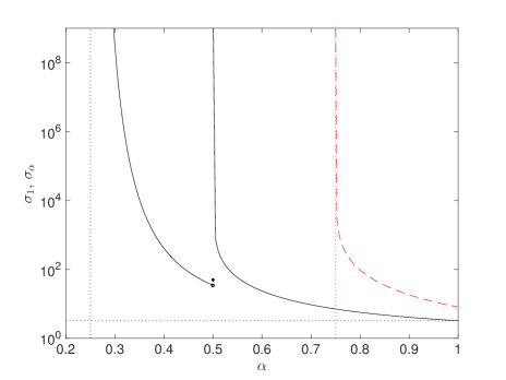
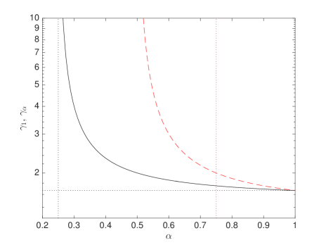
Figure 1: Constant prefactors $\sigma_{1}$, $\sigma_{\alpha}$ (a) and exponents $\gamma_{1}$, $\gamma_{\alpha}$ (b) of upper bounds (18) (black solid lines) and (24) (red dashed lines) as functions of the fractional dissipation exponent $\alpha$. The vertical dashed lines correspond to $\alpha=1/4$ and $3/4$, whereas the horizontal dashed lines represent the prefactors and exponents from estimate (7) corresponding to $\alpha=1$ [8, 9]. The viscosity coefficient is $\nu=0.01$.

3 Methodology for Probing Sharpness of Estimates (18) and (24)

In this section we discuss the approach which will allow us to verify whether or not the upper bounds (18) and (24) on the rate of growth of the classical and fractional enstrophy are sharp. An estimate of the type (18) or (24) is considered “sharp” when the upper bound on its right-hand side can be realized by certain fields $u$ with prescribed (classical or fractional) enstrophy. In other words, in regard to estimate (18), if we can find a family of fields $\tilde{u}_{\bar{{\mathcal{E}}}}$ such that ${\mathcal{E}}(\tilde{u}_{\bar{{\mathcal{E}}}})=\bar{{\mathcal{E}}}$ and ${\mathcal{R}}_{{\mathcal{E}}}(\tilde{u}_{\bar{{\mathcal{E}}}})\rightarrow\sigma_{1}\,\bar{{\mathcal{E}}}^{\gamma_{1}}$ when $\bar{{\mathcal{E}}}\rightarrow\infty$, then this estimate is declared sharp (analogously for estimate (24)). We note that, given the power-law structure of the upper bounds in (18) and (24), the question of sharpness may apply independently to both the exponents $\gamma_{1}$ and $\gamma_{\alpha}$ as well as the prefactors $\sigma_{1}$ and $\sigma_{\alpha}$ (with the caveat that if the exponent is not sharp, then the question about sharpness of the corresponding prefactor becomes moot). A natural way to systematically search for fields saturating an estimate is by solving suitable variational maximization problems [8, 9, 19, 23] and such problems corresponding to estimates (18) and (24) are introduced below.

3.1 Variational Formulation

For given $\bar{{\mathcal{E}}}>0$ and $\bar{{\mathcal{E}}}_{\alpha}>0$ on the RHS in estimates (18) and (24), we define the respective maximizers as

$${\widetilde{u}_{\bar{{\mathcal{E}}}}}=\operatorname*{arg\,max}\limits_{u\in{\mathcal{S}_{\bar{{\mathcal{E}}}}}}\mathcal{R}_{\mathcal{E}}(u)\,,$$ (26)

$${\mathcal{S}_{\bar{{\mathcal{E}}}}}=\left\{u\in H^{1+\alpha}(\mathcal{I}):\frac{1}{2}\int_{0}^{1}{\left|u_{x}\right|}^{2}\,dx={\bar{{\mathcal{E}}}}\right\}\,,$$

and

$${\widetilde{u}_{\bar{{\mathcal{E}}}_{\alpha}}}=\operatorname*{arg\,max}\limits_{u\in{\mathcal{S}_{\bar{{\mathcal{E}}}_{\alpha}}}}\mathcal{R}_{\mathcal{E}_{\alpha}}(u)\,,$$ (27)

$${\mathcal{S}_{\bar{{\mathcal{E}}}_{\alpha}}}=\left\{\begin{aligned} &\left\{u\in H^{2\alpha}(\mathcal{I}):\frac{1}{2}\int_{0}^{1}{\left|{(-\Delta)}^{\frac{\alpha}{2}}u\right|}^{2}\,dx={\bar{{\mathcal{E}}}_{\alpha}}\right\}&\qquad&\text{for}\ \alpha>\frac{1}{2},\\ &\left\{u\in H^{1}(\mathcal{I}):\frac{1}{2}\int_{0}^{1}{\left|{(-\Delta)}^{\frac{\alpha}{2}}u\right|}^{2}\,dx={\bar{{\mathcal{E}}}_{\alpha}}\right\}&&\text{for}\ \alpha\leq\frac{1}{2},\end{aligned}\right.$$

where “$\operatorname*{arg\,max}$” denotes the state realizing the maximum, whereas ${\mathcal{S}_{\bar{{\mathcal{E}}}}}$ and ${\mathcal{S}_{\bar{{\mathcal{E}}}_{\alpha}}}$ represent the constraint manifolds. The choice of the Sobolev spaces in the definitions of these manifolds is dictated by the minimum regularity of $u$ required in order to make the expressions for ${\mathcal{R}}_{{\mathcal{E}}}(u)$ and ${\mathcal{R}}_{{\mathcal{E}}_{\alpha}}(u)$, cf. (11) and (12), well defined. While establishing rigorously the solvability of optimization problems (26) and (27), especially for large values of $\bar{{\mathcal{E}}}$ and $\bar{{\mathcal{E}}}_{\alpha}$, is a difficult task (which is outside the scope of the present study), the computational results reported in Section 4 indicate that the maxima defined by these problems are indeed attained. A numerical approach to solution of maximization problems (26) and (27) is presented below.

3.2 Gradient-Based Solution of Problems (26) and (27)

To fix attention, we first focus on the solution of problem (26). For a fixed $\bar{{\mathcal{E}}}$, its maximizers can be computed as ${\widetilde{u}_{\bar{{\mathcal{E}}}}}=\lim_{n\rightarrow\infty}u^{(n)}$, where the consecutive approximations $u^{(n)}$ are defined via the following iterative procedure (in practice, only a finite number of iterations is performed)

$$u^{(n+1)} =\mathbb{P}\mathcal{S}\left(u^{(n)}+\tau_{n}\nabla^{H^{1+\alpha}}\mathcal{R}_{\mathcal{E}}(u^{(n)})\right),\qquad n=1,2,\dots,$$ (28a)

$$u^{(1)} =u^{0}\,,$$ (28b)

in which $u^{0}$ is the initial guess chosen such that $u^{0}\in{\mathcal{S}_{\bar{{\mathcal{E}}}}}$ and $\int_{0}^{1}u^{0}\,dx=0$, $\nabla^{H^{1+\alpha}}{\mathcal{R}}_{{\mathcal{E}}}(u^{(n)})$ is the Sobolev gradient of ${\mathcal{R}}_{{\mathcal{E}}}(u)$ evaluated at the $n$th iteration with respect to the suitable Sobolev topology, $\tau_{n}$ is the corresponding length of the step and $\mathbb{P}\mathcal{S}\;:\;H^{1+\alpha}({\mathcal{I}})\rightarrow{\mathcal{S}_{\bar{{\mathcal{E}}}}}$ is the projection operator ensuring that every iterate $u^{(n)}$ is restricted to the constraint manifold ${\mathcal{S}_{\bar{{\mathcal{E}}}}}$. For simplicity of presentation, in (28a) we used the steepest-ascent approach, however, in practice one can use a more advanced maximization approach characterized by faster convergence, such as for example the conjugate gradients method [34]. For the maximization problem (27) the maximizer $\widetilde{u}_{\bar{{\mathcal{E}}}_{\alpha}}$ can be computed with an algorithm similar to (28), but involving the constraint manifold $\mathcal{S}_{\bar{{\mathcal{E}}}_{\alpha}}$, the gradient $\nabla^{{H^{2\alpha}}}{\mathcal{R}}_{{\mathcal{E}}_{\alpha}}$ (or, $\nabla^{{H^{1}}}{\mathcal{R}}_{{\mathcal{E}}_{\alpha}}$) and the projection operator $\mathbb{P}\mathcal{S}_{\alpha}$, all of which are defined below.

As regards evaluation of the gradients $\nabla^{H^{1+\alpha}}{\mathcal{R}}_{{\mathcal{E}}}$ and $\nabla^{{H^{2\alpha}}}{\mathcal{R}}_{{\mathcal{E}}_{\alpha}}$ (or, $\nabla^{{H^{1}}}{\mathcal{R}}_{{\mathcal{E}}_{\alpha}}$), the starting point are the Gâteaux differentials of the objective functions $\eqref{eq:R}$ and (12), defined as

$$\mathcal{R}^{\prime}_{\mathcal{E}}(u;v):=\lim_{\epsilon\rightarrow 0}\frac{\mathcal{R}_{\mathcal{E}}(u+\epsilon v)-\mathcal{R}_{\mathcal{E}}(u)}{\epsilon}\quad\text{and}\quad\mathcal{R}^{\prime}_{\mathcal{E}_{\alpha}}(u;v):=\lim_{\epsilon\rightarrow 0}\frac{\mathcal{R}_{\mathcal{E}_{\alpha}}(u+\epsilon v)-\mathcal{R}_{\mathcal{E}_{\alpha}}(u)}{\epsilon}$$

which can be evaluated as follows

$$\mathcal{R}^{\prime}_{\mathcal{E}}(u;v) =\int_{0}^{1}\left[3u_{x}u_{xx}+2\nu{(-\Delta)}^{\alpha}u_{xx}\right]v\,dx\,,$$ (29a)

$$\mathcal{R}^{\prime}_{\mathcal{E}_{\alpha}}(u;v) =\int_{0}^{1}\left[{(-\Delta)}^{\alpha}u_{x}\cdot u-{(-\Delta)}^{\alpha}(u\cdot u_{x})-2\nu{(-\Delta)}^{2\alpha}u\right]v\,dx\,,$$ (29b)

where integration by parts has been used to factorize the “direction” $v$. Next, recognizing that, for a fixed $u$ and when regarded as functions of the second argument $v$, the Gâteaux differentials (29a)–(29b) are bounded linear functionals on the given Sobolev spaces, we can invoke the Riesz theorem [35] to obtain

$$\mathcal{R}^{\prime}_{{\mathcal{E}}}(u;v) ={\left\langle\nabla^{L^{2}}\mathcal{R}_{\mathcal{E}}(u),v\right\rangle}_{L^{2}(\mathcal{I})} ={\left\langle\nabla^{H^{1+\alpha}}\mathcal{R}_{\mathcal{E}}(u),v\right\rangle}_{H^{1+\alpha}(\mathcal{I})}\,,$$ (30a)

$$\mathcal{R}^{\prime}_{{\mathcal{E}}_{\alpha}}(u;v) ={\left\langle\nabla^{L^{2}}\mathcal{R}_{{\mathcal{E}}_{\alpha}}(u),v\right\rangle}_{L^{2}(\mathcal{I})} ={\left\langle\nabla^{H^{2\alpha}}\mathcal{R}_{{\mathcal{E}}_{\alpha}}(u),v\right\rangle}_{H^{2\alpha}(\mathcal{I})}, \quad\text{for}\ \alpha>\frac{1}{2}\,,$$ (30b)

$$={\left\langle\nabla^{H^{1}}\mathcal{R}_{{\mathcal{E}}_{\alpha}}(u),v\right\rangle}_{H^{1}(\mathcal{I})}, \quad\text{for}\ \alpha\leq\frac{1}{2}\,,$$ (30c)

where the Sobolev inner products are defined as

$${\left\langle u,v\right\rangle}_{H^{1+\alpha}(\mathcal{I})} :=\int_{0}^{1}u\,v+\ell_{1}^{2}u_{x}\,v_{x}+\ell_{2}^{2+2\alpha}{(-\Delta)}^{\frac{\alpha}{2}}u_{x}\cdot{(-\Delta)}^{\frac{\alpha}{2}}v_{x}\,dx\,,$$ (31a)

$${\left\langle u,v\right\rangle}_{H^{2\alpha}(\mathcal{I})} :=\int_{0}^{1}u\,v+\ell_{1}^{2}u_{x}\,v_{x}+\ell_{2}^{4\alpha}{(-\Delta)}^{\alpha-\frac{1}{2}}u_{x}\cdot{(-\Delta)}^{\alpha-\frac{1}{2}}v_{x}\,dx\,,$$ (31b)

$${\left\langle u,v\right\rangle}_{H^{1}(\mathcal{I})} :=\int_{0}^{1}u\,v+\ell_{1}^{1}u_{x}v_{x}\,dx\,$$ (31c)

in which $\ell_{1}$ and $\ell_{2}$ are constants with the dimension of a length-scale (the significance of the choice of these constants will be discussed below). In order to characterize the Sobolev gradients defined in the spaces $H^{1+\alpha}({\mathcal{I}})$, $H^{2\alpha}({\mathcal{I}})$ and $H^{1}({\mathcal{I}})$, cf. (26)–(27), we first derive expressions for the $L^{2}$ gradients from (29a)–(29b)

$$\nabla^{L^{2}}\mathcal{R}_{\mathcal{E}}(u) =3u_{x}u_{xx}+2\nu{(-\Delta)}^{\alpha}u_{xx}\,,$$ (32a)

$$\nabla^{L^{2}}\mathcal{R}_{\mathcal{E}_{\alpha}}(u) ={(-\Delta)}^{\alpha}u_{x}\cdot u-{(-\Delta)}^{\alpha}(u\cdot u_{x})-2\nu{(-\Delta)}^{2\alpha}u$$ (32b)

and then invoke Riesz relations (30a)–(30c) which, upon performing integration by parts and noting that $v$ is arbitrary, yields

$$\left[{1}-l_{1}^{2}\Delta-l_{2}^{2+2\alpha}{(-\Delta)}^{\alpha}\Delta\right]\nabla^{H^{1+\alpha}}\mathcal{R}_{\mathcal{E}}(u) =\nabla^{L^{2}}\mathcal{R}_{\mathcal{E}}(u)\,, \text{on}\ {\mathcal{I}},$$ (33a)

$$\left[{1}-l_{1}^{2}\Delta-l_{2}^{4\alpha}{(-\Delta)}^{2\alpha-1}\Delta\right]\nabla^{H^{2\alpha}}\mathcal{R}_{\mathcal{E}_{\alpha}}(u) =\nabla^{L^{2}}\mathcal{R}_{\mathcal{E}_{\alpha}}(u)\,, \text{on}\ {\mathcal{I}},$$ (33b)

$$\left[{1}-l_{1}^{2}\Delta\right]\nabla^{H^{1}}\mathcal{R}_{\mathcal{E}_{\alpha}}(u) =\nabla^{L^{2}}\mathcal{R}_{\mathcal{E}_{\alpha}}(u)\,, \text{on}\ {\mathcal{I}},$$ (33c)

Periodic Boundary Conditions.

These boundary-value problems allow us to determine the required Sobolev gradients in terms of the $L^{2}$ gradients (32a)–(32b). We now return to the question of the choice of the length-scale parameters $\ell_{1}$ and $\ell_{2}$. As is evident from the form of these expressions, for different values of $\ell_{1}$ and $\ell_{2}$ inner products (31a)–(31c) define equivalent norms as long as $\ell_{1},\ell_{2}\in(0,\infty)$. On the other hand, as demonstrated in [36], computation of Sobolev gradients by solving elliptic boundary-value problems (33a)–(33c) can be interpreted as application of spectral low-pass filters to the $L^{2}$ gradients with the parameters $\ell_{1}$ and $\ell_{2}$ defining the cut-off length-scales. Thus, while for sufficiently “good” initial guesses $u^{0}$ iterations of the type (28) with different values of $\ell_{1}$ and $\ell_{2}$ lead to the same maximizer $\widetilde{u}_{\bar{{\mathcal{E}}}}$, the actual rate of convergence usually depends very strongly on the choice of these parameters [19, 23].

Since the constraints defining the manifolds in (26) and (27) are quadratic, the corresponding projection operators are naturally defined in terms of the following rescalings (normalizations)

$$\mathbb{P}\mathcal{S}(u) :=\sqrt{\frac{{\bar{{\mathcal{E}}}}}{\frac{1}{2}\int_{0}^{1}{|u_{x}|}^{2}\,dx}}\ u\,,$$ (34a)

$$\mathbb{P}\mathcal{S}_{\alpha}(u) :=\sqrt{\frac{{\bar{{\mathcal{E}}}_{\alpha}}}{\frac{1}{2}\int_{0}^{1}{\big{|}{(-\Delta)}^{\frac{\alpha}{2}}u\big{|}}^{2}\,dx}}\ u\$$ (34b)

which in the language of optimization on manifolds can be interpreted as “retractions” from the tangent subspace to the constraint manifold [37]. The form of expressions (34a) and (34b) is particularly simple, because the constraint manifolds ${\mathcal{S}_{\bar{{\mathcal{E}}}}}$ and ${\mathcal{S}_{\bar{{\mathcal{E}}}_{\alpha}}}$, cf. (26) and (27), can be regarded as “spheres” in their respective functional spaces. Finally, the optimal step length $\tau_{n}$ in (28) is found by solving an arc-minimization problem

$$\tau_{n}:=\operatorname*{arg\,max}\limits_{\tau>0}\left\{\mathcal{R}_{\mathcal{E}}\left[\mathbb{P}\mathcal{S}\left(u^{(n)}+\tau\nabla^{H^{1+\alpha}}\mathcal{R}_{\mathcal{S}}(u^{(n)})\right)\right]\right\}\,$$ (35)

which is an adaptation of standard line minimization [34] to the case with quadratic constraints. This step is performed with a straightforward generalization of Brent’s method [38] and an analogous approach is also used to compute the step size when solving problem (27).

3.3 Tracing Solutions Branches via Continuation

Families of maximizers $\widetilde{u}_{\bar{{\mathcal{E}}}}$ corresponding to a range of enstrophy values ${\bar{{\mathcal{E}}}}={\mathcal{E}}^{(m)}$, $m=0,1,\dots$, are obtained using a continuation approach where the solution $\widetilde{u}_{{\mathcal{E}}^{(m)}}$ determined by the iteration process (28) at some enstrophy value ${\mathcal{E}}^{(m)}$ is used as the initial guess $u^{0}$ for iterations at the next, slightly larger, value ${\mathcal{E}}^{(m+1)}={\mathcal{E}}^{(m)}+\Delta{\mathcal{E}}$ for some $\Delta{\mathcal{E}}>0$. By choosing sufficiently small steps $\Delta{\mathcal{E}}$, one can ensure that the iterations at a given enstrophy value are rapidly convergent. The same continuation approach is also used to compute the families of the maximizers $\widetilde{u}_{\bar{{\mathcal{E}}}_{\alpha}}$.

3.4 Rates of Growth of Enstrophy for $\alpha=0$

To close this section, we provide some comments about the rates of growth of the classical and fractional enstrophy in the case when $\alpha=0$. As regards the first quantity, from (11) we see that

$${\mathcal{R}}_{{\mathcal{E}}}(u)\,\leq\,\frac{1}{2}\|u_{x}\|_{L^{3}({\mathcal{I}})}^{3}-\nu\|u_{x}\|_{L^{2}({\mathcal{I}})}^{2}$$ (36)

which, in view of the property $\|v\|_{L^{p}({\mathcal{I}})}\leq\|v\|_{L^{q}({\mathcal{I}})}$ true for $p\leq q$ [18], implies that for $u\in\mathcal{S}_{{\mathcal{E}}}$, ${\mathcal{R}}_{{\mathcal{E}}}(u)$ may not be bounded and hence the maximization problem (26) does not have solutions when $\alpha=0$. Concerning the rate of growth of the fractional enstrophy, from (12) we obtain

$$\frac{d{\mathcal{K}}(u)}{dt}=-{\mathcal{K}}(u),$$ (37)

where ${\mathcal{K}}(u):={\mathcal{E}}_{0}(u)=(1/2)\int_{0}^{1}u^{2}\,dx$ is the kinetic energy and we used the property that $\int_{0}^{1}uuu_{x}\,dx=0$. Then, the maximization problem (27) takes the form $\max_{u,\;{\mathcal{K}}(u)={\bar{{\mathcal{K}}}}}\left[-{\mathcal{K}}(u)\right]$ for some ${\bar{{\mathcal{K}}}}>0$, and it is clear that any function $u\in H^{1}({\mathcal{I}})$ such that ${\mathcal{K}}(u)={\bar{{\mathcal{K}}}}$ is a solution. Thus, when $\alpha=0$, the maximization problem (27) has infinitely many solutions.

4 Computational Results

In this section we present and analyze the results obtained by solving problems (26) and (27) for a broad range of $\bar{{\mathcal{E}}}$ and $\bar{{\mathcal{E}}}_{\alpha}$ and for different values of the fractional dissipation exponent $\alpha\in[0,1]$. We begin by describing the numerical techniques employed to discretize the approach introduced in Section 3.2 and then summarize the values of the different numerical parameters used.

For a given field $u$, the gradient expressions (32a)–(32b) are evaluated using a spectrally accurate Fourier-Galerkin approach in which the nonlinear terms are computed in the physical space with dealiasing based on the $2/3$ rule [39]. A similar Fourier-Galerkin approach is also used to solve the boundary-value problems (33a)–(33c) for the Sobolev gradients. As will be discussed in more detail below, the maximizers $\widetilde{u}_{\bar{{\mathcal{E}}}}$ and $\widetilde{u}_{\bar{{\mathcal{E}}}_{\alpha}}$ corresponding to increasing values of, respectively, $\bar{{\mathcal{E}}}$ and $\bar{{\mathcal{E}}}_{\alpha}$ are characterized by shock-like steep fronts of decreasing thickness. Resolving these regions accurately requires numerical resolutions (given in terms of the numbers $N$ of Fourier modes) increasing with $\bar{{\mathcal{E}}}$ and $\bar{{\mathcal{E}}}_{\alpha}$. In our computations we used the resolutions $N=512,\dots,8388608$ which were refined adaptively based on the criterion that the Fourier coefficients corresponding to several largest resolved wavenumbers be at the level of the round-off errors, i.e., $|\hat{u}_{k}|\sim\mbox{{O}}(10^{-14})$ for $k\lessapprox N$. By carefully performing such grid refinement it was possible to assert that in all cases the computed approximations converge to well-defined maximizers. In all cases considered the viscosity was set to $\nu=0.01$. The length-scale parameters $\ell_{1}$ and $\ell_{2}$ in the definitions of the Sobolev inner products (31) were chosen to maximize the rate of convergence of iterations (28) for given values of $\alpha$, $\bar{{\mathcal{E}}}$ or $\bar{{\mathcal{E}}}_{\alpha}$. The best results were obtained for $\ell_{1}\in[1,10]$ and $\ell_{2}\in[10^{-6},1]$ with smaller values corresponding to larger $\bar{{\mathcal{E}}}$ and $\bar{{\mathcal{E}}}_{\alpha}$. Since the gradient-based method from Section 3.2 may find local maximizers only, in addition to the continuation approach described in Section 3.3, we have also started iterations (28) with several different initial guesses $u^{0}$ intended to nudge the iterations towards other possible local maximizers (typically, $u^{0}(x)=A\sin(2\pi kx)$ with $k=1,2,\dots$ and $A$ chosen so that ${\mathcal{E}}(u^{0})$ or ${\mathcal{E}}_{\alpha}(u^{0})$ was equal to a prescribed value). However, these attempts did not reveal any additional maximizers other than the ones already found using the continuation approach.

4.1 Maximum Growth Rate of Classical Enstrophy

We consider solutions to maximization problem (26) for $\alpha\in(1/4,1]$, which is the range of fractional dissipation exponents for which estimate (18) is valid. The maximum rate of growth ${\mathcal{R}}_{{\mathcal{E}}}({\widetilde{u}_{\bar{{\mathcal{E}}}}})$ is shown as a function of $\bar{{\mathcal{E}}}$ for different values of $\alpha$ in Figure 2. In this figure we also indicate the upper bounds from estimate (18). The corresponding maximizers $\widetilde{u}_{\bar{{\mathcal{E}}}}$ are shown both in the physical and spectral space in Figure 3 for ${\bar{{\mathcal{E}}}}=5,50,500$ and $\alpha\in[0.5,1]$. It is evident from this figure that the sharp fronts in these maximizers become steeper with increasing $\bar{{\mathcal{E}}}$ and this effect is more pronounced for smaller values of $\alpha$. This aspect is further illustrated in Figure 4 where the maximizers are shown for $\alpha=0.3,0.4$ and small enstrophy values. Needless to say, accurate determination of maximizers $\widetilde{u}_{\bar{{\mathcal{E}}}}$ for such small values of the fractional dissipation exponent $\alpha$ requires a very refined numerical resolution, cf. Figure 4(d), making the optimization problem (26) harder and more costly to solve. This also explains why for small values of $\alpha$ the data for ${\mathcal{R}}_{{\mathcal{E}}}({\widetilde{u}_{\bar{{\mathcal{E}}}}})$ in Figure 2 is available only for small $\bar{{\mathcal{E}}}$. The relation ${\mathcal{R}}_{{\mathcal{E}}}({\widetilde{u}_{\bar{{\mathcal{E}}}}})$ versus $\bar{{\mathcal{E}}}$ is characterized by certain generic properties evident for all values of $\alpha$ — while for small $\bar{{\mathcal{E}}}$ the quantity ${\mathcal{R}}_{{\mathcal{E}}}({\widetilde{u}_{\bar{{\mathcal{E}}}}})$ exhibits a steep growth with $\bar{{\mathcal{E}}}$, for larger values of $\bar{{\mathcal{E}}}$ it develops a power-law dependence on $\bar{{\mathcal{E}}}$. This behavior can be quantified by fitting the relation ${\mathcal{R}}_{{\mathcal{E}}}({\widetilde{u}_{\bar{{\mathcal{E}}}}})$ versus $\bar{{\mathcal{E}}}$ locally with the formula $\widetilde{\sigma}_{1}{\bar{{\mathcal{E}}}}^{\widetilde{\gamma}_{1}}$ and determining the parameters $\widetilde{\sigma}_{1}$ and $\widetilde{\gamma}_{1}$ as functions of $\bar{{\mathcal{E}}}$ via a least-squares procedure. The dependence of thus determined prefactor $\widetilde{\sigma}_{1}$ and exponent $\widetilde{\gamma}_{1}$ on $\bar{{\mathcal{E}}}$ is shown for different $\alpha$ in Figures 5(a,c,e) and 5(b,d,f), respectively. In these figures we also indicate the values of $\sigma_{1}$ and $\gamma_{1}$ obtained in estimate (18). We observe, that as $\bar{{\mathcal{E}}}$ increases, both the prefactor and the exponent obtained via the least-squares fit approach well-defined limiting values. These limiting values are then compared against the relations $\sigma_{1}=\sigma_{1}(\alpha)$ and $\gamma_{1}=\gamma_{1}(\alpha)$ from estimate (18) in Figures 6(a,b). It is clear from Figure 6(b) that there is a good quantitative agreement between the exponent in estimate (18) and the computational results. On the other hand, in Figure 6(a) we see that the numerically determined prefactors are smaller than the prefactor derived in estimate (18), although they do exhibit similar trends with $\alpha$ (except for the discontinuity of the latter at $\alpha=1/2$). This demonstrates that exponent $\gamma_{1}$ in estimate (18) is sharp, while prefactor $\sigma_{1}$ might be improved. We add that we also attempted to solve the maximization problem (26) for $\alpha\in(0,1/4]$, however, we were unable to obtain converged solutions. In agreement with the discussion of the case $\alpha=0$ in Section 3.4, this indicates that $d{\mathcal{E}}/dt$ may be unbounded for $\alpha\leq 1/4$.

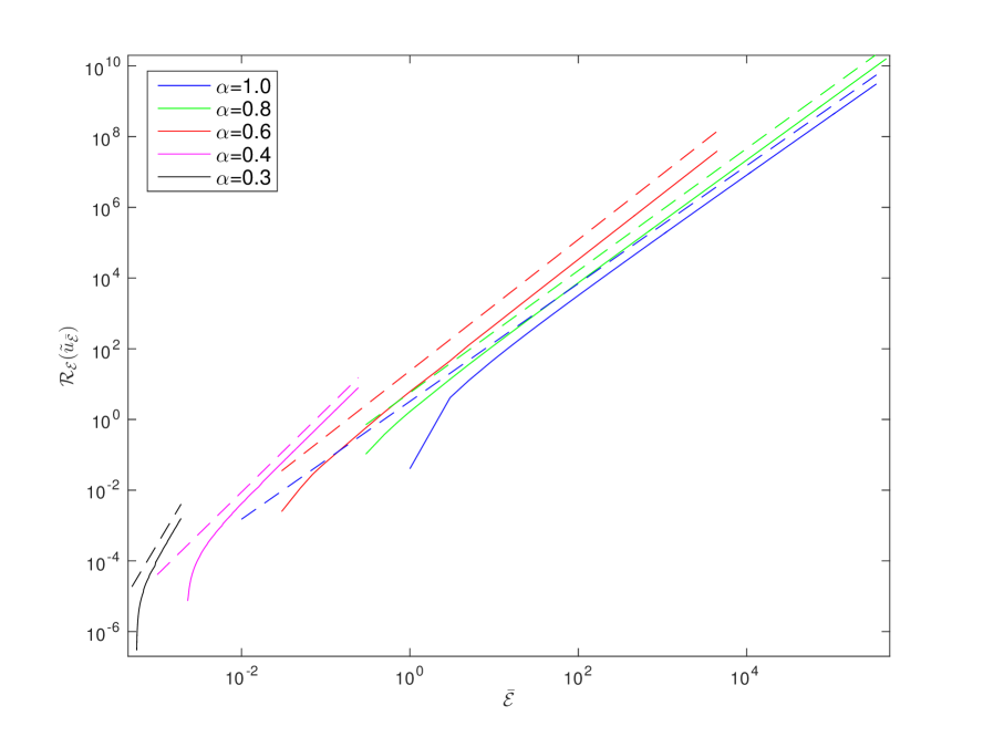
Figure 2: Dependence of the maximum enstrophy rate of growth ${\mathcal{R}}_{{\mathcal{E}}}({\widetilde{u}_{\bar{{\mathcal{E}}}}})$, obtained by solving optimization problems (26), on $\bar{{\mathcal{E}}}$ for different values of $\alpha$ (solid lines). The dashed lines represent the corresponding upper bounds from estimate (18).

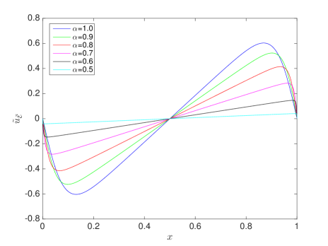
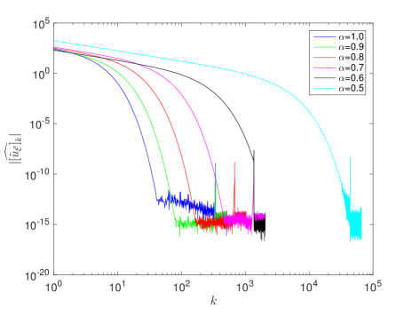
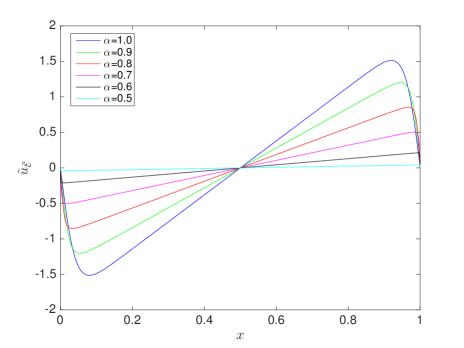
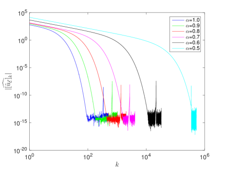
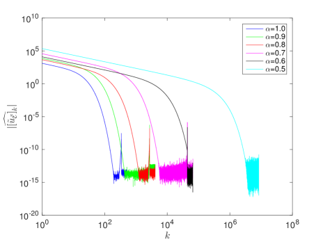
Figure 3: Maximizers $\widetilde{u}_{\bar{{\mathcal{E}}}}$ obtained for ${\bar{{\mathcal{E}}}}=5$ (a,b), ${\bar{{\mathcal{E}}}}=50$ (c,d) and ${\bar{{\mathcal{E}}}}=500$ (e,f) and different values of $\alpha$. The fields are shown in the physical (a,c,e) and spectral (b,d,f) space.

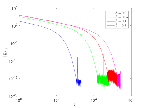
Figure 4: Maximizers $\widetilde{u}_{\bar{{\mathcal{E}}}}$ obtained for $\alpha=0.4$ (a,b) and $\alpha=0.3$ (c,d) and different values of $\bar{{\mathcal{E}}}$. The fields are shown in the physical (a,c) and spectral (b,d) space.

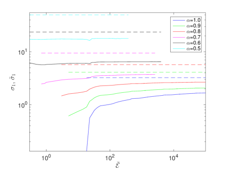
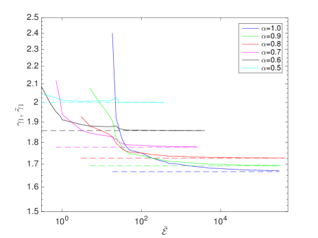
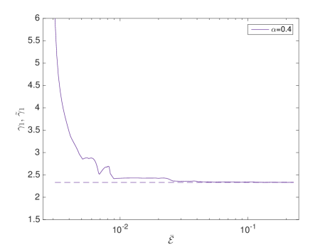
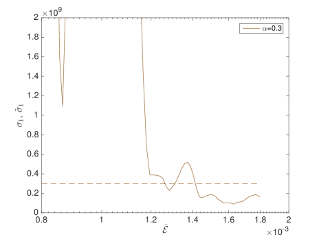
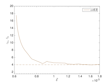
Figure 5: Prefactors $\widetilde{\sigma}_{1}$ (a,c,e) and exponents $\widetilde{\gamma}_{1}$ (b,d,f) obtained as function of $\bar{{\mathcal{E}}}$ via local least-squares fits to the relations ${\mathcal{R}}_{{\mathcal{E}}}({\widetilde{u}_{\bar{{\mathcal{E}}}}})$ versus $\bar{{\mathcal{E}}}$ shown in Figure 2 (solid lines). The dashed lines represent the corresponding prefactors $\sigma_{1}$ and exponents $\gamma_{1}$ from estimate (18).

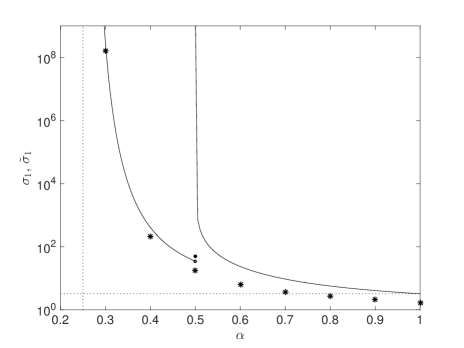
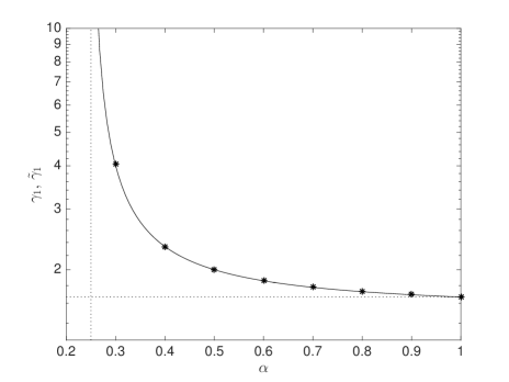
Figure 6: Prefactors (a) and exponents (b) in the power-law relation $\widetilde{\sigma}_{1}{\bar{{\mathcal{E}}}}^{\widetilde{\gamma}_{1}}$ describing the dependence of ${\mathcal{R}}_{{\mathcal{E}}}({\widetilde{u}_{\bar{{\mathcal{E}}}}})$ on $\bar{{\mathcal{E}}}$ shown as functions of $\alpha$: limiting (as ${\bar{{\mathcal{E}}}}\rightarrow\infty$, cf. Figure 5) values obtained in the least-squares fits (symbols) and predictions of estimate (18) (solid lines).

4.2 Maximum Growth Rate of Fractional Enstrophy

While estimate (24) was established for $\alpha\in(3/4,1]$, in order to obtain insights about the maximum growth rate of the fractional enstrophy for a broad range of fractional dissipation exponents, in this section we solve the maximization problems (27) for $\alpha\in[0,1]$. The obtained maximum growth rate ${\mathcal{R}}_{{\mathcal{E}}_{\alpha}}({\widetilde{u}_{\bar{{\mathcal{E}}}_{\alpha}}})$ is shown as a function of $\bar{{\mathcal{E}}}_{\alpha}$ in Figures 8(a) and 8(b) for $\alpha\in(3/4,1]$ and $\alpha\in(1/10,3/4]$, respectively. In the first figure we also indicate the predictions of estimate (24). For small values of $\alpha$ and $\bar{{\mathcal{E}}}_{\alpha}$ we also observed the presence of another branch of maximizers characterized by negative values of ${\mathcal{R}}_{{\mathcal{E}}_{\alpha}}({\widetilde{u}_{\bar{{\mathcal{E}}}_{\alpha}}})$ — this data is shown in Figure 8(a) using a restricted range of $\bar{{\mathcal{E}}}_{\alpha}$ for clarity, whereas the positive branches obtained for the same (small) values of $\alpha$ are presented in Figure 8(b). We thus see that for small $\alpha$ and $\bar{{\mathcal{E}}}_{\alpha}$ the maximization problem (27) admits two distinct families of local maximizers. The maximizers $\widetilde{u}_{\bar{{\mathcal{E}}}_{\alpha}}$ corresponding to the data in Figures 8(a,b) are shown both in the physical and spectral space in Figure 9 for ${\bar{{\mathcal{E}}}_{\alpha}}=5,50,500$ and $\alpha=0.1,0.2,\dots,0.9$. We observe that, interestingly, as $\alpha$ decreases the sharp fronts in the maximizers disappear and are replaced with oscillations (Figures 9(a,c,e)). This behavior is also reflected in the spectra of the maximizers which become less developed as $\alpha\rightarrow 0$ (Figures 9(b,d,f)). The maximizers $\widetilde{u}_{\bar{{\mathcal{E}}}_{\alpha}}$ obtained at the same values of $\alpha$ and $\bar{{\mathcal{E}}}_{\alpha}$, and corresponding to the positive and negative branches of ${\mathcal{R}}_{{\mathcal{E}}_{\alpha}}({\widetilde{u}_{\bar{{\mathcal{E}}}_{\alpha}}})$, cf. Figures 8(a) and 8(b), are shown in Figure 10. We see that the maximizers for which ${\mathcal{R}}_{{\mathcal{E}}_{\alpha}}({\widetilde{u}_{\bar{{\mathcal{E}}}_{\alpha}}})<0$ have a simpler structure and for all considered values of $\alpha$ and $\bar{{\mathcal{E}}}_{\alpha}$ are essentially indistinguishable from $A\sin(2\pi x)$ for some $A>0$. The relation ${\mathcal{R}}_{{\mathcal{E}}_{\alpha}}({\widetilde{u}_{\bar{{\mathcal{E}}}_{\alpha}}})$ versus $\bar{{\mathcal{E}}}_{\alpha}$ (the upper branch shown in Figure 8(a,b)) reveals similar properties as observed in the case of the classical enstrophy discussed in Section 4.1, namely, an initially steep growth followed by saturation with a power-law behavior when ${\bar{{\mathcal{E}}}_{\alpha}}\rightarrow\infty$. Performing local least-squares fits to these relations with the formula $\widetilde{\sigma}_{\alpha}{\bar{{\mathcal{E}}}_{\alpha}}^{\widetilde{\gamma}_{\alpha}}$, as described in Section 4.1, we can calculate how the actual prefactors $\widetilde{\sigma}_{\alpha}$ and exponents $\widetilde{\gamma}_{\alpha}$ depend on $\bar{{\mathcal{E}}}_{\alpha}$ and these results are shown in Figure 11(a,b), where we have also indicated, for $\alpha\in(3/4,1]$, the predictions of estimate (24). We see that, as ${\bar{{\mathcal{E}}}_{\alpha}}\rightarrow\infty$, both $\widetilde{\sigma}_{\alpha}$ and $\widetilde{\gamma}_{\alpha}$ approach well-defined values, which are in turn shown in Figure 12(a,b) as functions of $\alpha$ together with the prefactors and the exponents obtained in estimate (24). We see in Figure 12(b) that for $0.9\lessapprox\alpha\lessapprox 1$ the numerically obtained exponents $\widetilde{\gamma}_{\alpha}$ match the exponents $\gamma_{\alpha}$ from estimate (24) and a difference appears for $0.8\lessapprox\alpha\lessapprox 0.9$ which grows as $\alpha$ decreases. For $0.7\lessapprox\alpha\lessapprox 0.8$ the numerically determined exponents $\widetilde{\gamma}_{\alpha}$ are a decreasing function of $\alpha$ which saturates at a constant value of approximately $3/2$ when $\alpha\lessapprox 0.7$. At the same time, the prefactors $\widetilde{\sigma}_{\alpha}$ obtained numerically are by a few orders of magnitude smaller than the prefactors predicted by estimate (24) over the entire range of $\alpha$, although they do exhibit qualitatively similar trends with $\alpha$. For $\alpha\in[0,3/4]$, which is outside the range of validity of estimate (24), the numerically obtained exponents $\widetilde{\gamma}_{\alpha}$ are constant, indicating that, somewhat surprisingly, in this range ${\mathcal{R}}_{{\mathcal{E}}_{\alpha}}({\widetilde{u}_{\bar{{\mathcal{E}}}_{\alpha}}})$ does not depend on the fractional dissipation exponent $\alpha$. The corresponding numerically obtained prefactors $\widetilde{\sigma}_{\alpha}$ reveal a decreasing trend with $\alpha$. We add that these trends are accompanied by the maximizers $\widetilde{u}_{\bar{{\mathcal{E}}}_{\alpha}}$ becoming more regular as $\alpha$ decreases (cf. Figure 9). We thus conclude that the exponent $\gamma_{\alpha}$ in estimate (24) is sharp over a part of the range of validity of this estimate and appears to overestimate the actual rate of growth of fractional enstrophy for smaller values of $\alpha$. Over the range of $\alpha$ where the exponent $\gamma_{\alpha}$ is sharp, the prefactor $\sigma_{\alpha}$ may be improved.

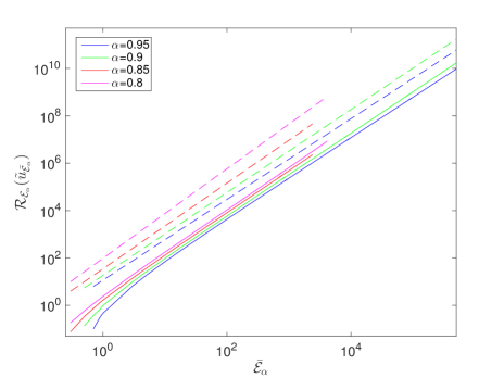
Figure 7: Dependence of the maximum fractional enstrophy rate of growth ${\mathcal{R}}_{{\mathcal{E}}_{\alpha}}({\widetilde{u}_{\bar{{\mathcal{E}}}_{\alpha}}})$, obtained by solving optimization problems (27), on $\bar{{\mathcal{E}}}_{\alpha}$ (solid lines) for $\alpha\in(3/4,1]$ (a) and $\alpha\in(1/10,3/4]$ (b). The dashed lines in panel (a) represent the corresponding upper bounds from estimate (24).

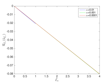
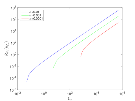
Figure 8: Dependence of the maximum fractional enstrophy rate of growth ${\mathcal{R}}_{{\mathcal{E}}_{\alpha}}({\widetilde{u}_{\bar{{\mathcal{E}}}_{\alpha}}})$, obtained by solving optimization problems (27), on $\bar{{\mathcal{E}}}_{\alpha}$ for small values of $\alpha$: negative branch (a) and positive branch (b).

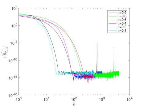
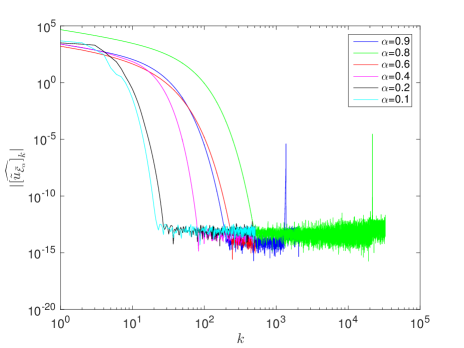
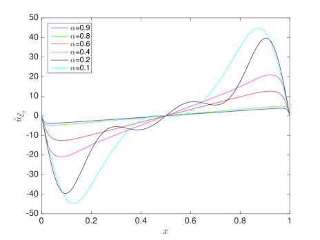
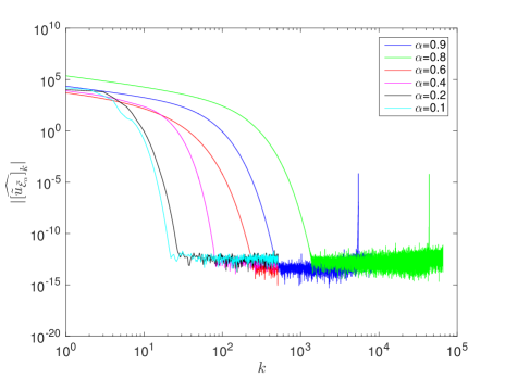
Figure 9: Maximizers $\widetilde{u}_{\bar{{\mathcal{E}}}_{\alpha}}$ obtained for ${\bar{{\mathcal{E}}}_{\alpha}}=5$ (a,b), ${\bar{{\mathcal{E}}}_{\alpha}}=50$ (c,d) and ${\bar{{\mathcal{E}}}_{\alpha}}=500$ (e,f) and different values of $\alpha$. The fields are shown in the physical (a,c,e) and spectral (b,d,f) space.

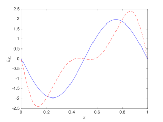
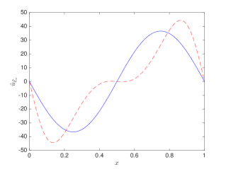
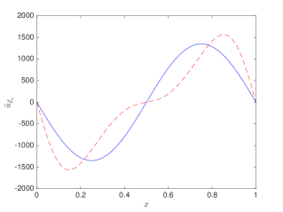
Figure 10: The maximizers $\widetilde{u}_{\bar{{\mathcal{E}}}_{\alpha}}$ characterized by positive ${\mathcal{R}}_{{\mathcal{E}}_{\alpha}}({\widetilde{u}_{\bar{{\mathcal{E}}}_{\alpha}}})$ (red dashed lines) and negative ${\mathcal{R}}_{{\mathcal{E}}_{\alpha}}({\widetilde{u}_{\bar{{\mathcal{E}}}_{\alpha}}})$ (blue solid lines) obtained for (a) ${\bar{{\mathcal{E}}}_{\alpha}}=1$, $\alpha=0.01$, (b) ${\bar{{\mathcal{E}}}_{\alpha}}=335$, $\alpha=0.001$, and (c) ${\bar{{\mathcal{E}}}_{\alpha}}=455,000$, $\alpha=0.0001$.

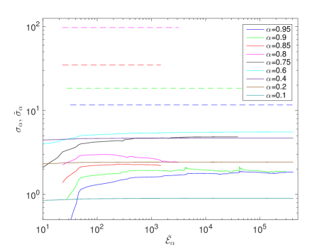
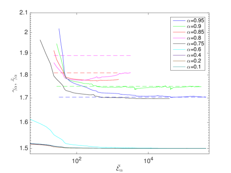
Figure 11: Prefactors $\widetilde{\sigma}_{\alpha}$ (a) and exponents $\widetilde{\gamma}_{\alpha}$ (b) obtained as function of $\bar{{\mathcal{E}}}_{\alpha}$ via local least-squares fits to the relation ${\mathcal{R}}_{{\mathcal{E}}_{\alpha}}({\widetilde{u}_{\bar{{\mathcal{E}}}_{\alpha}}})$ versus $\bar{{\mathcal{E}}}_{\alpha}$ shown Figure 8 (solid lines). The dashed lines represent the corresponding prefactors $\sigma_{\alpha}$ and exponents $\gamma_{\alpha}$ from estimate (24).

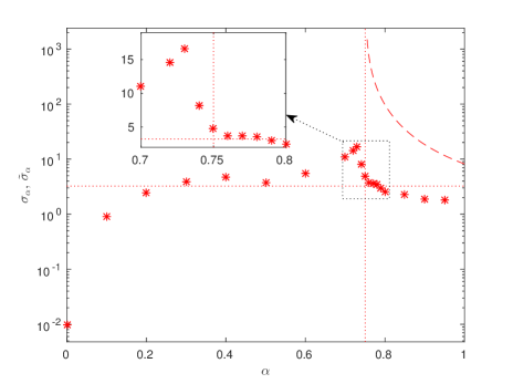
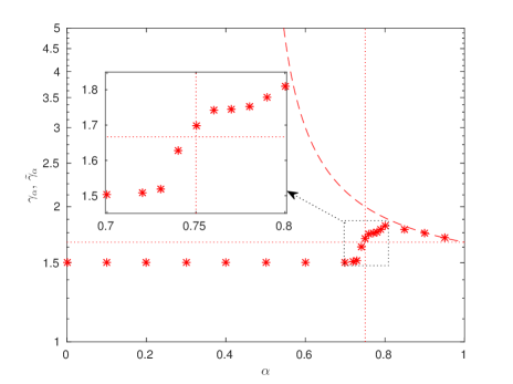
Figure 12: Prefactors (a) and exponents (b) in the power-law relation $\widetilde{\sigma}_{\alpha}{\bar{{\mathcal{E}}}_{\alpha}}^{\widetilde{\gamma}_{\alpha}}$ describing the dependence of ${\mathcal{R}}_{{\mathcal{E}}_{\alpha}}({\widetilde{u}_{\bar{{\mathcal{E}}}_{\alpha}}})$ on $\bar{{\mathcal{E}}}_{\alpha}$ shown as functions of $\alpha$: limiting (as ${\bar{{\mathcal{E}}}_{\alpha}}\rightarrow\infty$, cf. Figure 11) values obtained in the least-squares fits (symbols) and predictions of estimate (24) (dashed lines). The insets represent magnifications of the neighborhood of $\alpha=3/4$ where estimate (24) loses its validity.

5 Summary and Discussion

While the estimates on the rate of growth of the classical and fractional enstrophy obtained in Theorems 2.1 and 2.2 are not much different from similar results already available in the literature [26, 27], the key finding of the present study is that these estimates are in fact sharp, in the sense that for different $\alpha$ the exponents $\gamma_{1}$ and $\gamma_{\alpha}$ in (18) and (24) capture the correct power-law dependence of the maximum growth rates ${\mathcal{R}}_{{\mathcal{E}}}({\widetilde{u}_{\bar{{\mathcal{E}}}}})$ and ${\mathcal{R}}_{{\mathcal{E}}_{\alpha}}({\widetilde{u}_{\bar{{\mathcal{E}}}_{\alpha}}})$ on $\bar{{\mathcal{E}}}$ and $\bar{{\mathcal{E}}}_{\alpha}$, respectively (the second estimate was found to be sharp only over a part of the range of $\alpha$ for which it is defined). This was demonstrated by computationally solving suitably defined constrained optimization problems and then showing that the maximizers obtained under constraints on ${\mathcal{E}}$ and ${\mathcal{E}}_{\alpha}$ saturate the upper bounds in the estimates for different values of $\alpha$. Therefore, the conclusion is that the mathematical analysis on which Theorems 2.1 and 2.2 are based may not be fundamentally improved, other than a refinement of exponent $\gamma_{\alpha}$ in (24) for $3/4<\alpha\lessapprox 0.9$ and an improvement of the prefactors in (18) and (24).

In regard to the maximum rate of growth of the classical enstrophy, it was found that for $\alpha\rightarrow(1/4)^{+}$ the exponent $\gamma_{1}$ in estimate (18) becomes unbounded, cf. Figure 6(b), which together with the computational evidence obtained for $\alpha\in[0,1/4]$ suggests that $d{\mathcal{E}}/dt$ may be unbounded for $\alpha$ in this range. This would indicate that for $\alpha\in[0,1/4]$ system (3) is not even locally well posed in $H^{1}({\mathcal{I}})$.

Concerning the maximum rate of growth of the fractional enstrophy, a surprising result was obtained for $\alpha\in[0,3/4)$, where the exponent in the upper bound on $d{\mathcal{E}}_{\alpha}/dt$ was found to be independent of $\alpha$ (cf. Figure 12(b)). This indicates that, unlike in the case of the classical enstrophy, in this range of $\alpha$ the problem does not become more singular with the decrease of $\alpha$ and this is in fact also reflected in the maximizers $\widetilde{u}_{\bar{{\mathcal{E}}}_{\alpha}}$ becoming more regular as $\alpha\rightarrow 0$. In addition, this also suggests that it should be possible to obtain rigorous bounds on $d{\mathcal{E}}_{\alpha}/dt$ valid for $\alpha\leq 3/4$, although they would likely need to be derived using techniques other than those employed in the proof of Theorem 2.2.

It should be emphasized that although most of the individual inequalities used in the proofs of Theorems 2.1 and 2.2 are known to be sharp, the fact that the upper bounds in (18) and (24) were found to be sharp as well is not trivial. This is because, in general, these individual inequalities may be saturated by different fields which may belong to different function spaces and hence it is not obvious whether sharpness is preserved when these inequalities are “chained” together to form estimates (18) and (24).

On the methodological side, it ought to be emphasized that gradient-based iterations (28) may only identify local maximizers and in general it is not possible to ascertain whether these maximizers are also global. However, our careful search based on the continuation approach (cf. Section 3.3) and, independently, using several different initial guesses $u^{0}$ did not reveal any additional maximizers (other than the maximizers obtained via a trivial rescaling of the solutions as discussed in detail in [19]). An exception to this was the solution of the maximization problem (27) for small $\alpha$ and $\bar{{\mathcal{E}}}_{\alpha}$ where a branch of maximizers such that ${\mathcal{R}}_{{\mathcal{E}}_{\alpha}}({\widetilde{u}_{\bar{{\mathcal{E}}}_{\alpha}}})<0$ was also found. The presence of this additional branch appears related to the degenerate nature of the maximization problem (27) which for $\alpha=0$ has an uncountable infinity of trivial solutions (cf. Section 3.4).

As regards the research program discussed in Introduction, the key finding of the present study is that exponents $\gamma_{1}$ in the upper bound on $d{\mathcal{E}}/dt$ have the same dependence on $\alpha$ and remain sharp in the subcritical, critical and parts of the supercritical regime. Thus, the loss of global well-posedness as $\alpha$ is reduced to values below $1/2$ cannot be detected based on the instantaneous rate of growth of enstrophy $d{\mathcal{E}}/dt$. The most important open problem related to the present study concerns obtaining the corresponding estimates for the finite-time growth of ${\mathcal{E}}(u(t))$ and ${\mathcal{E}}_{\alpha}(u(t))$ and verifying their sharpness. This question can be addressed using the approach developed in [19] and will be investigated in future research.

References

• [1] H. Kreiss and J. Lorenz. Initial-Boundary Value Problems and the Navier-Stokes Equations, volume 47 of Classics in Applied Mathematics. SIAM, 2004.
• [2] C. R. Doering. The 3D Navier-Stokes problem. Annual Review of Fluid Mechanics, 41:109–128, 2009.
• [3] C. L. Fefferman. Existence and smoothness of the Navier-Stokes equation. available at http://www.claymath.org/sites/default/files/navierstokes.pdf, 2000. Clay Millennium Prize Problem Description.
• [4] Jean Leray. Sur le mouvement d’un liquide visqu’eux emplissant l’espace. Acta Mathematica, 63(1):193–248, 1934.
• [5] J. D. Gibbon, M. Bustamante, and R. M. Kerr. The three–dimensional Euler equations: singular or non–singular? Nonlinearity, 21:123–129, 2008.
• [6] C. Foias and R. Temam. Gevrey class regularity for the solutions of the Navier–Stokes equations. Journal of Functional Analysis, 87:359–369, 1989.
• [7] J. T. Beale, T. Kato, and A. Majda. Remarks on the breakdown of smooth solutions for the $3$-d euler equations. Comm. Math. Phys., 94(1):61–66, 1984.
• [8] L. Lu. Bounds on the enstrophy growth rate for solutions of the 3D Navier-Stokes equations. PhD thesis, University of Michigan, 2006.
• [9] L. Lu and C. R. Doering. Limits on enstrophy growth for solutions of the three-dimensional Navier–Stokes equations. Indiana University Mathematics Journal, 57:2693–2727, 2008.
• [10] D. Ayala and B. Protas. Extreme vortex states and the growth of enstrophy in 3D incompressible flows. Journal of Fluid Mechanics, 818:772–806, 2017.
• [11] O. N. Boratav and R. B. Pelz. Direct numerical simulation of transition to turbulence from a high-symmetry initial condition. Physics of Fluids, 6:2757–2784, 1994.
• [12] R. B. Pelz. Symmetry and the hydrodynamic blow-up problem. Journal of Fluid Mechanics, 444:299–320, 2001.
• [13] K. Ohkitani and P. Constantin. Numerical study of the Eulerian–Lagrangian analysis of the Navier-Stokes turbulence. Phys. Fluids, 20:1–11, 2008.
• [14] P. Orlandi, S. Pirozzoli, and G. F. Carnevale. Vortex events in Euler and Navier-Stokes simulations with smooth initial conditions. Journal of Fluid Mechanics, 690:288–320, 2012.
• [15] Diego A. Donzis, John D. Gibbon, Anupam Gupta, Robert M. Kerr, Rahul Pandit, and Dario Vincenzi. Vorticity moments in four numerical simulations of the 3D Navier-Stokes equations. Journal of Fluid Mechanics, 732:316–331, 2013.
• [16] G. Luo and T. Y. Hou. Potentially Singular Solutions of the 3D Axisymmetric Euler Equations. Proceedings of the National Academy of Sciences, 111(36):12968–12973, 2014.
• [17] G. Luo and T. Y. Hou. Toward the Finite-Time Blowup of the 3D Incompressible Euler Equations: a Numerical Investigation. SIAM: Multiscale Modeling and Simulation, 12(4):1722–1776, 2014.
• [18] R. A. Adams and J. F. Fournier. Sobolev Spaces. Elsevier, 2005.
• [19] D. Ayala and B. Protas. On maximum enstrophy growth in a hydrodynamic system. Physica D, 240:1553–1563, 2011.
• [20] D. Pelinovsky. Sharp bounds on enstrophy growth in the viscous Burgers equation. Proceedings of Royal Society A, 468:3636–3648, 2012.
• [21] D. Pelinovsky. Enstrophy growth in the viscous Burgers equation. Dynamics of Partial Differential Equations, 9:305–340, 2012.
• [22] D. Poccas and B. Protas. Transient Growth in Stochastic Burgers Flows. arXiv:1510.05037, 2016.
• [23] D. Ayala and B. Protas. Maximum palinstrophy growth in 2D incompressible flows. Journal of Fluid Mechanics, 742:340–367, 2014.
• [24] D. Ayala and B. Protas. Vortices, maximum growth and the problem of finite-time singularity formation. Fluid Dynamics Research, 46(3):031404, 2014.
• [25] N. Alibaud, J. Droniou, and J. Vovelle. Occurrence and non-appearance of shocks in fractal Burgers equations. J. Hyperbolic Differ. Equ., 4:479–499, 2007.
• [26] A. Kiselev, F. Nazaraov, and R. Shterenberg. Blow up and regularity for fractal Burgers equation Dynamics of Partial Differential Equations. Dynamics of Partial Differential Equations, 5:211–240, 2008.
• [27] H. J. Dong, D. P. Du, and D. Li. Finite time singularities and global well-posedness for fractal Burgers equations. Indiana Univ. Math. J., 58:807–821, 2009.
• [28] C. H. Chan, M. Czubak, and L. Silvestre. Eventual Regularization of The Slightly Supercritical Fractional Burgers Equation. Discrete and Continuous Dynamical Systems A, 27:847–861, 2010.
• [29] J. Arias. Simulation of hydrodynamic models exhibiting singularity formation in finite time. Master’s project report, McMaster University, 2015.
• [30] N.H. Katz and N. Pavlović. A cheap Caffarelli-Kohn-Nirenberg inequality for the Navier-Stokes equation with hyper-dissipation. Geometric & Functional Analysis GAFA, 12(2):355–379, 2002.
• [31] H. Hajaiej, X. W. Yu, and Z. C. Zhai. Fractional Gagliardo-Nirenberg and Hardy inequalities under Lorentz norms. J. Math. Anal. Appl., 396:569–577, 2012.
• [32] D. S. McCormick, J. C. Robinson, and J. L. Rodrigo. Generalised Gagliardo-Nirenberg Inequalities Using Weak Lebesgue Spaces and BMO. Milan Journal of Mathematics, 81:265–289, 2013.
• [33] H. Hajaiej, L. Molinet, T. Ozawa, and B. X. Wang. Necessary and sufficient conditions for the fractional Gagliardo-Nirenberg inequalities and applications to Navier-Stokes and generalized boson equations. RIMS Kokyuroku Bessatsu, 26:159–199, 2011.
• [34] J. Nocedal and S. J. Wright. Numerical Optimization. Springer, 1999.
• [35] D. Luenberger. Optimization by Vector Space Methods. John Wiley and Sons, 1969.
• [36] B. Protas, T. Bewley, and G. Hagen. A comprehensive framework for the regularization of adjoint analysis in multiscale PDE systems. Journal of Computational Physics, 195:49–89, 2004.
• [37] P.-A. Absil, R. Mahony, and R. Sepulchre. Optimization Algorithms on Matrix Manifolds. Princeton University Press, 2008.
• [38] W. H. Press, B. P. Flannery, S. A. Teukolsky, and W. T. Vetterling. Numerical Recipes. Cambridge University Press, 1986.
• [39] J. P. Boyd. Chebyshev and Fourier Spectral Methods. Dover, 2001.