Excitation of H${}_{2}^{+}$ with one-cycle laser pulses: Shaped post-laser-field electronic oscillations, generation of higher- and lower-order harmonics

Abstract

Non Born-Oppenheimer quantum dynamics of H${}_{2}^{+}$ excited by shaped one-cycle laser pulses linearly polarized along the molecular axis have been studied by the numerical solution of the time-dependent Schrödinger equation within a three-dimensional model, including the internuclear separation, $R$, and the electron coordinates $z$ and $\rho$. Laser carrier frequencies corresponding to the wavelengths $\lambda_{l}=25$ nm through $\lambda_{l}=400$ nm were used and the amplitudes of the pulses were chosen such that the energy of H${}_{2}^{+}$ was close to its dissociation threshold at the end of any laser pulse applied. It is shown that there exists a characteristic oscillation frequency $\omega_{\rm osc}\simeq 0.2265$ au (corresponding to the period of $\tau_{\rm osc}\simeq 0.671$ fs and the wavelength of $\lambda_{\rm osc}\simeq 200$ nm) that manifests itself as a “carrier” frequency of temporally shaped oscillations of the time-dependent expectation values $\langle z\rangle$ and $\langle\partial V/\partial z\rangle$ that emerge at the ends of the laser pulses and exist on a timescale of at least 50 fs. Time-dependent expectation values $\langle\rho\rangle$ and $\langle\partial V/\partial\rho\rangle$ of the optically-passive degree of freedom, $\rho$, demonstrate post-laser-field oscillations at two basic frequencies $\omega^{\rho}_{1}\approx\omega_{\rm osc}$ and $\omega^{\rho}_{2}\approx 2\omega_{\rm osc}$. Power spectra associated with the electronic motion show higher- and lower-order harmonics with respect to the driving field.

1 Introduction

Coherent oscillations of bound particles (electrons or muons) that persist after laser field excitation of a molecule  [1, 2, 3] is an interesting new phenomenon, which generalizes the well-known recollision model of Corkum [4] to the case when high-order harmonics are generated due to coherent oscillations of bound electrons or muons after the end of the laser field that induced their motion. Coherent post-laser-field oscillations of bound particles were found to exist both in ordinary (electronic) and muonic molecules, as shown by numerical propagation of the respective non-Born-Oppenheimer time-dependent Schrödinger equations [1, 2, 3].

Coherent post-laser-field electronic oscillations were first found in the heavy molecular ion T${}_{2}^{+}$ after its excitation by a UV laser pulse [1]. Subsequently [2], coherent and shaped post-laser-field oscillations of a muon were found in muonic $dd\mu$ and $dt\mu$ molecules after their excitation by super-intense attosecond soft X-ray laser pulses at the wavelength of $\lambda_{l}=5$ nm. It was found, in particular, that only odd harmonics were generated in the homonuclear $dd\mu$ molecule by the optically active $z$ degree of freedom, as suggested by the concept of inversion symmetry [5]. Only even harmonics were generated in $dd\mu$ by the optically passive, transversal $\rho$ degree of freedom, which is excited only due to the wave properties of an electron. In contrast, both odd and even harmonics were generated in the heteronuclear $dt\mu$ molecule by the optically active $z$ degree of freedom due to inversion symmetry breaking [5], and both even and odd harmonics were generated in $dt\mu$ by the optically passive $\rho$ degree of freedom. It was also shown in Ref. [2] that the appearance of coherent muonic oscillations in $dd\mu$ and $dt\mu$ after the end of the laser field is a purely non-Born-Oppenheimer effect: the post-laser-field muonic oscillations did not occur if the Born-Oppenheimer approximation was employed.

In our recent work [3], shaped post-laser-field electronic oscillations were also found to exist in H${}_{2}^{+}$ excited by two-cycle laser pulses at the wavelengths $\lambda_{l}=800$ and 200 nm. It was shown, in particular, that there exists a characteristic oscillation frequency $\omega_{\rm osc}=0.2278$ au (corresponding to the wavelength of $\lambda_{l}=200$ nm) that plays the role of a “carrier” frequency of temporally shaped post-laser-field electronic oscillations both at $\lambda_{l}=800$ nm and at $\lambda_{l}=200$ nm. In the present work, we investigate the non-Born-Oppenheimer quantum dynamics of H${}_{2}^{+}$ excited by shaped one-cycle laser pulses, i.e. the shortest periodic excitation of H${}_{2}^{+}$ is studied. The laser carrier frequencies corresponding to the wavelengths $\lambda_{l}=25$, 50, 100 150, 200, 300 and 400 nm are used such as as to cover the domains of both $\omega_{l}\leq\omega_{\rm osc}$ and $\omega_{l}>\omega_{\rm osc}$. Similarly to our previous work [3], the amplitudes of one-cycle laser pulses are chosen such that the energy of H${}_{2}^{+}$ after the ends of the pulses are $\langle E\rangle\simeq-0.515$ au, i.e., slightly below its dissociation threshold $E_{\rm D}=-0.5$ au.

2 Model, equations of motion, and numerical methods

The three-body three-dimensional model with the Coulombic interactions representing the ${\rm H}_{2}^{+}$ excited by the laser field linearly polarized along the $z$ axis is shown in Figure 1. The nuclear motion is assumed to be restricted to the polarization direction of the laser electric field. The electron (${\rm e}$) moves in three dimensions with conservation of cylindrical symmetry. Therefore, only two electronic coordinates, $z$ and $\rho$, measured with respect to the center of mass of the two protons (${\rm p}$) should be treated explicitly together with the internuclear separation $R$.

Figure 1: The three-body three-dimensional model of ${\rm H}_{2}^{+}$ excited by a laser field linearly polarized along the $z$ axis. The internuclear distance is $R$, the distances between the electron and each of the two protons are $r_{1}$ and $r_{2}$, see Equations (4) and (5).

The component of the dipole moment of ${\rm H}_{2}^{+}$ along the $z$ axis reads [6]

$$d_{z}(z)=-ez[1+M_{\rm e}/(2M_{\rm p}+M_{\rm e})],$$ (1)

where $-e$ is the electron charge, $M_{\rm p}$ and $M_{\rm e}$ are the proton and the electron masses, respectively. The homonuclear ${\rm H}_{2}^{+}$ molecular ion does not have a permanent dipole moment, therefore its vibrational motion is excited only indirectly due to electronic motion induced by the laser field along the $z$ axis [7, 8, 9]. Electronic motion along the transversal $\rho$ axis occurs only due to the wave properties of the electron.

The time-dependent non-Born-Oppenheimer Schrödinger equation that governs the quantum dynamics of ${\rm H}_{2}^{+}$ in the classical laser field ${\cal E}(t)$ reads

$$i\hbar\frac{\partial}{\partial t}\Psi-\frac{\hbar^{2}}{2m_{\rm n}}\frac{\partial^{2}\Psi}{\partial R^{2}}-\frac{\hbar^{2}}{2m_{\rm e}}\biggl{(}\frac{\partial^{2}\Psi}{\partial\rho^{2}}+\frac{1}{\rho}\frac{\partial\Psi}{\partial\rho}\biggr{)}$$

$$-\frac{\hbar^{2}}{2m_{\rm e}}\frac{\partial^{2}\Psi}{\partial z^{2}}+V(R,\rho,z)\Psi-d_{z}(z){\cal E}(t)\Psi.$$ (2)

In Equation (2), $m_{\rm n}=M_{\rm p}/2$ is the nuclear reduced mass, $m_{\rm e}=2M_{\rm e}M_{\rm p}/(M_{\rm e}+2M_{\rm p})$ is the electron reduced mass. In the atomic units (au) used throughout the paper, we have: $e=\hbar=M_{\rm e}=1$ and $m_{\rm e}\simeq 1$ and for the field amplitude and intensity ${\mathcal{E}}_{0}=5\times 10^{9}$ V/cm and $I_{0}=3.5\times 10^{16}$ W/cm², respectively.

The Coulomb potential reads

$$V(R,\rho,z)=e^{2}(1/R-1/r_{1}-1/r_{2}),$$ (3)

where the electron-proton distances (see Figure 1) are

$$r_{1}(R,\rho,z)=[\rho^{2}+(z+R/2)^{2}]^{1/2}$$ (4)

and

$$r_{2}(R,\rho,z)=[\rho^{2}+(z-R/2)^{2}]^{1/2}.$$ (5)

The time-dependent laser electric field ${\cal E}(t)$ is chosen as follows:

$${\cal E}(t)={\cal E}_{0}\sin^{2}(\pi t/t_{p})\sin(\omega_{l}t),\,\,\,\,\,\,0\leq t\leq t_{p},$$ (6)

where ${\cal E}_{0}$ is the amplitude, $t_{p}$ is the pulse duration at the base, and $\omega_{l}$ is the laser carrier frequency. With the symmetric (the $\sin^{2}$-type) envelope and the integer number of optical cycles at the base (one optical cycle in the present case), the laser electric field ${\cal E}(t)$ has a vanishing direct-current component, $\int_{0}^{t_{p}}{\cal E}(t)dt=0$, and satisfies therefore Maxwell’s equations in the propagation region [10]. Note before proceeding, that at a small number of optical cycles per pulse duration, as in the present work for example, the carrier-envelope phase (CEP) may play a very important role [11]. We shall address this issue in our future work. Here, we just assume that the carrier-envelope phase is equal to zero, see Equation (6).

The numerical methods used to solve the three-dimensional Equation (2) have been described in our previous works [8, 9]. In particular, the dissociation probability has been calculated with the time- and space-integrated outgoing flux for the nuclear coordinate $R$; the ionization probabilities have been calculated with the respective fluxes separately for the positive and the negative direction of the $z$ axis as well as for the outer end of the $\rho$ axis.

The size of the $z$-grid has been chosen such as to be substantially larger than the maximum electron excursion along the $z$ axis, $\alpha_{z}={\cal E}_{0}/\omega_{l}^{2}$, and the size of the $\rho$-grid has been chosen accordingly. The maximum electron excursion, $\alpha_{z}=9.25$ au, corresponds to the field parameters used at $\lambda_{l}=400$ nm (${\cal E}_{0}=0.12$ au and $\omega_{l}=0.1139$ au) and the choice of the $z$ and $\rho$ grids has been based on this value. Specifically, the three-dimensional wave-function $\Psi(t)$ of Equation (2) was damped with the imaginary smooth optical potentials, adapted from [12], at $z<-263$ au, at $z>263$ au and at $\rho>239$ au for the electronic motion, and at $R>23$ au for the nuclear motion.

Initially, at $t=0$, the ${\rm H}_{2}^{+}$ was assumed to be in its ground vibrational and ground electronic state. The wave function of the initial state was been obtained by the numerical propagation of Equation (2) in the imaginary time without the laser field (${\cal E}_{0}=0$).

3 Results

3.1 Resonant properties, laser-driven dynamics, and free evolution of ${\rm H}_{2}^{+}$ on a short timescale

As it was already mentioned, the amplitudes ${\cal E}_{0}$ of the one-cycle laser pulses used in the present work have been chosen such that the energies of ${\rm H}_{2}^{+}$ at the ends of the laser pulses were slightly below the dissociation threshold ($E_{D}=-0.5$ au) and similar, $\langle E(t=t_{p})\rangle\approx-0.515$ au. The amplitudes of one-cycle laser pulses required to achieve the aforementioned energy are plotted in Figure 2 versus their wavelength $\lambda_{l}$ by curve 1. For the sake of comparison, similar results obtained with two-cycle laser pulses are presented in Figure 2 by curve 2.

Figure 2: The amplitudes of one-cycle (curve 1) and two-cycle (curve 2) laser pulses required to excite ${\rm H}_{2}^{+}$ from its ground vibrational state $v=0$ to the energy of $\langle E\rangle\approx-0.515$ au.

Two different domains of the laser wavelength $\lambda_{l}$ can be clearly distinguished in Figure 2. The domain of a large change of the laser pulse amplitude ${\cal E}_{0}$ required to excite ${\rm H}_{2}^{+}$ to the energy of $\langle E\rangle\approx-0.515$ au with the laser wavelength $\lambda_{l}$ corresponds to $\lambda_{l}<200$ nm (or $\omega_{l}>\omega_{\rm osc}$). The domain of a relatively small change of ${\cal E}_{0}$ with $\lambda_{l}$ corresponds to $\lambda_{l}\geq 200$ nm ($\omega_{l}\leq\omega_{\rm osc}$). It is also seen from Figure 2 that the most efficient excitation of ${\rm H}_{2}^{+}$ by one-cycle and two-cycle laser pulses, which requires the minimum laser electric-field amplitude, takes place at $\lambda_{l}^{\rm opt}\simeq 200$ nm, which plays the role of a resonant, or the optimal laser wavelength. It can be expected therefore that power spectra of electron oscillations resulting from excitation of ${\rm H}_{2}^{+}$ to $\langle E\rangle\approx-0.515$ au at various laser wavelengths $\lambda_{l}\neq 200$ nm should always contain harmonics corresponding to $\lambda\approx 200$ nm.

Indeed, it was shown in our recent work [3], where excitation of ${\rm H}_{2}^{+}$ with two-cycle laser pulses at $\lambda_{l}=200$ and 800 nm was studied, that the respective power spectra contain the strongest harmonics corresponding to $\lambda=200$ nm, the fourth harmonic at $\lambda_{l}=800$ nm and the first (identical) harmonic at $\lambda_{l}=200$ nm. It will be interesting to check therefore whether the excitation of ${\rm H}_{2}^{+}$ with laser wavelengths $\lambda_{l}<200$ nm would result in the generation of lower-order harmonics.

An important problem of the laser-driven dynamics with few-cycle laser pulses is the electron-field following. According to the well-known recollision model of Corkum [4], electron follows the field out-of-phase: the expectation value $\langle z(t)\rangle$ decreases when electric-field strength ${\cal E}(t)$ increases. Previously, a perfect electron-field out-of-phase following on the level of expectation values $\langle z\rangle$ of the laser-driven electronic degree of freedom have been found only in the infrared [8, 9] and near-infrared [13] domains of the laser carrier frequency, with a large number of optical cycles per pulse duration $t_{p}$ being involved. It was also found in our previous work [14] that electrons of the extended H-H system follow the applied laser field out-of phase at the laser carrier frequency $\omega_{l}<0.1$ au, and in-phase at $\omega_{l}=1$ au, with the number of optical cycles per pulse duration being about 33.

The laser-driven dynamics of ${\rm H}_{2}^{+}$ excited by two-cycle laser pulses was studied in our recent work [3]. It was found, in particular, that at $\lambda_{l}=800$ nm, the expectation value $\langle z\rangle$ follows the field out-of-phase only approximately (during the first optical cycle), while at $\lambda_{l}=200$ nm, the out-of-phase electron-field following does not take place even approximately. It would be moreover difficult to expect the out-of-phase electron-field following for expectation values $\langle z\rangle$ at one-cycle excitation.

The laser-driven dynamics of ${\rm H}_{2}^{+}$ excited by one-cycle laser pulses at $\lambda_{l}=150$ and 300 nm is presented in Figure 3 on the timescale of 3 fs (left and right panel, respectively). It is seen from Figures 3(a), 3(b), 3(d) and 3(e) that electron approximately follows the laser field out-of-phase only during the first half-cycle, while during the second half-cycle of the laser pulse, the expectation value $\langle z\rangle$ may change even in-phase with the laser field. Nevertheless, after the ends of one-cycle laser pulses, expectation values $\langle z\rangle$ demonstrate rather regular oscillations with the period of $\tau_{\rm osc}\simeq 0.667$ fs corresponding to the wavelength $\lambda_{\rm osc}\simeq 200$ nm and frequency $\omega_{\rm osc}\simeq 0.2278$ au.

Figure 3: Quantum dynamics of ${\rm H}_{2}^{+}$ excited by the one-cycle laser pulses at $\lambda_{l}=150$ nm (a-c) and $\lambda_{l}=300$ nm (d-f). Parameters of the laser pulses: (a) ${\cal E}_{0}=0.088$ au, $\omega_{l}=0.30376$ au, $t_{p}=0.5$ fs; (d) ${\cal E}_{0}=0.045$ au, $\omega_{l}=0.15188$ au, $t_{p}=1.0$ fs; (b,e) time-dependent expectation values $\langle z\rangle$; (c,f) time-dependent expectation values $\langle\rho\rangle$.

The transversal electron degree of freedom, $\rho$, is optically passive if the laser field is aligned along the $z$ axis (Figure 1). It can be excited therefore only due to the wave properties of electron. The time-dependent expectation values $\langle\rho\rangle$ at laser wavelengths $\lambda_{l}=150$ and 300 nm are presented in Figures 3(c) and (f), respectively. It is seen that expectation values $\langle\rho\rangle$ start to increase at the end of the first optical half-cycle and demonstrates quite regular (yet not harmonic) oscillations during the second optical half-cycle and after the ends of the one-cycle laser pulses. Two major frequencies of $\rho$-oscillations can be distinguished at a close look. Indeed, time intervals between two highest maxima of $\rho$-oscillations in Figures 3(c) and (f) are $\tau^{\rm osc}_{1}\approx 0.667$ fs, corresponding to the frequency of $\omega^{\rho}_{1}\approx\omega_{\rm osc}$, or the wavelength of $\lambda^{\rho}_{1}\approx 200$ nm. On the other hand, time intervals between the neighboring maxima of $\rho$-oscillations in Figures 3(c) and (f), are $\tau^{\rm osc}_{2}\approx 0.334$ fs, corresponding to the frequency of $\omega^{\rho}_{2}\approx 2\omega_{\rm osc}$, or the wavelength of $\lambda^{\rho}_{2}\approx 100$ nm.

While the appearance of electronic $\rho$-oscillations with the frequency $\omega^{\rho}_{1}\approx\omega_{\rm osc}$ being very close to the frequency of electronic $z$-oscillations could be expected, the “frequency-doubling” of electronic $\rho$-oscillations occurring at $\omega^{\rho}_{2}\approx 2\omega_{\rm osc}$ needs more explanations. Such a frequency-doubling of electronic $z$-oscillations by its $\rho$-oscillations occurring at $\omega^{\rho}_{2}\approx 2\omega_{\rm osc}$ was explained in our previous works [8, 9] as follows. During electronic oscillations along the $z$ axis, the electronic density is substantially delocalized also in the transversal, $\rho$ direction, due to the wave properties of the electron. This takes place at every turning point of electronic $z$-oscillations, i.e., twice per every cycle of electronic $z$-oscillations, giving rise to excitation of ${\rm H}_{2}^{+}$ along the $\rho$ axis in a stepwise manner. Similar frequency-doubling of muonic oscillation also takes place in muonic $dd\mu$ and $dt\mu$ molecules excited by super-intense soft X-ray laser pulses at the wavelength of $\lambda_{l}=5$ nm on the attosecond timescale [2].

The characteristic feature of the post-laser-field electronic $z$-oscillations in ${\rm H}_{2}^{+}$ excited by one-cycle laser pulses is their asymmetry with respect to $\langle z\rangle=0$ [Figures 3(b) and (e)]. This is especially evident on a longer timescale in comparison with smoothly shaped oscillations of expectation values $\langle-\partial V/\partial z\rangle$, as shown in Figure 4 on the timescale of 12 fs. The left panel presents expectation values $\langle z\rangle$ at the laser wavelength $\lambda_{l}=150$ nm (a) and $\lambda_{l}=300$ nm (b). The right panel presents expectation values $\langle-\partial V/\partial z\rangle$ at $\lambda_{l}=150$ nm (c) and $\lambda_{l}=300$ nm (d). Post-field oscillations of $\langle-\partial V/\partial z\rangle$ occur with the same frequency, $\omega_{\rm osc}\simeq 0.2278$ au (corresponding to the wavelength $\lambda_{\rm osc}\simeq 200$ nm) as those of $\langle z\rangle$. The existence of coherent post-laser-field oscillations of $\langle z\rangle$ and $\langle-\partial V/\partial z\rangle$ in ${\rm H}_{2}^{+}$ excited to the energy of $\langle E\rangle\simeq-0.515$ au by two-cycle laser pulses was rationalized in detail in our recent work [3] where approximately the same characteristic oscillation frequency was calculated. Thus in the present case of one-cycle laser pulses similar arguments hold true to explain the appearance of post-laser-field electronic oscillations. Note that the characteristic oscillation frequency corresponding to $\lambda_{\rm osc}\approx 200$ nm is in line with the results presented in Figure 2 evidencing the most efficient excitation of ${\rm H}_{2}^{+}$ to $\langle E\rangle\simeq-0.515$ au at the laser wavelength of $\lambda_{l}\approx 200$ nm. Also note that asymmetry of time-dependent expectation values $\langle z\rangle$ with respect to $\langle z\rangle=0$ implies the time-dependent polarization of ${\rm H}_{2}^{+}$ after its excitation by one-cycle laser pulses.

Figure 4: Quantum dynamics of ${\rm H}_{2}^{+}$ excited by the one-cycle laser pulses at $\lambda_{l}=150$ nm (a,c) and $\lambda_{l}=300$ nm (b,d) followed by coherent post-laser-field electronic oscillations: (a,b) time-dependent expectation values $\langle z\rangle$; (c,d) time-dependent expectation values $\langle-\partial V/\partial z\rangle$. Parameters of the laser pulses are as in Figure 3.

3.2 Ionization, dissociation and post-laser-field electronic oscillations of ${\rm H}_{2}^{+}$ on a long timescale

Numerical simulations of the laser-driven quantum dynamics and subsequent free evolution of ${\rm H}_{2}^{+}$ were performed as long as ionization and dissociation probabilities were small enough, not more than about 2%.

Figure 5: Ionization and dissociation probabilities of ${\rm H}_{2}^{+}$ excited by one-cycle laser pulse at the wavelength $\lambda_{l}=25$ nm. Curve 1 — ionization probability for the outer end of the $\rho$ axis; curves 2 and 3 — ionization probabilities for the negative and the positive direction of the $z$ axis, respectively; curve 4 — dissociation probability. Parameters of the laser pulse: ${\cal E}_{0}=1.18$ au, $\omega_{l}=1.8225$ au, $t_{p}\simeq 0.0833$ fs.

The time-dependent ionization and dissociation probabilities are presented in Figure 5 on the timescale of 50 fs for the case when ${\rm H}_{2}^{+}$ is excited by one-cycle laser pulse at the laser wavelength $\lambda_{l}=25$ nm. Note that ionization probabilities have been calculated with the respective time- and space-integrated outgoing fluxes separately for the negative and the positive direction of the $z$ axis (curves 2 and 3, respectively) as well as for the outer end of the $\rho$ axis (curve 1). The dissociation probability (curve 4) has been similarly calculated for the nuclear coordinate $R$.

Since the optimal laser-pulse amplitude required to prepare ${\rm H}_{2}^{+}$ at the energy of $\langle E\rangle\approx-0.515$ au at the laser wavelength $\lambda_{l}=25$ nm is substantially larger than at larger wavelengths, both dissociation and ionization probabilities presented in Figure 5 are the largest obtained in this work. It is seen from Figure 5 that the ionization probability for the outer end of the $\rho$ axis is larger than those for both negative and positive direction of the $z$ axis. This can be explained by the aforementioned fact that the electronic density is delocalized in the $\rho$ direction twice per every cycle of electronic $z$-oscillations, giving rise to the frequency-doubling of electronic $\rho$-oscillations as compared to electronic $z$-oscillations. It is also seen from Figure 5 that ionization starts much prior to dissociation, therefore ‘ionizative dissociation’ occurs. Indeed, the decrease of the electron density between the two protons due to ionization disturbs the initial equilibrium configuration of ${\rm H}_{2}^{+}$ and thus allows the Coulombic repulsion of the protons to act more efficiently resulting in the elongation of the internuclear distance in ${\rm H}_{2}^{+}$ and its subsequent dissociation.

Figure 6: The time-dependent expectation values $\langle R\rangle$ for ${\rm H}_{2}^{+}$ excited by the one-cycle laser pulses at $\lambda_{l}=25$ nm (curve 1, ${\cal E}_{0}=1.18$ au, $\omega_{l}=1.8225$ au, $t_{p}\simeq 0.0833$ fs), $\lambda_{l}=50$ nm (curve 2, ${\cal E}_{0}=0.625$ au, $\omega_{l}=0.91127$ au, $t_{p}\simeq 0.167$ fs), $\lambda_{l}=100$ nm (curve 3, ${\cal E}_{0}=0.174$ au, $\omega_{l}=0.45563$ au, $t_{p}\simeq 0.333$ fs) and $\lambda_{l}=200$ nm (curve 4, ${\cal E}_{0}=0.06$ au, $\omega_{l}=0.22782$ au, $t_{p}\simeq 0.667$ fs).

The time-dependent expectation values $\langle R\rangle$ of internuclear distances in ${\rm H}_{2}^{+}$ are presented in Figure 6 on the timescale of 50 fs for the laser wavelengths of $\lambda_{l}=25$ nm (curve 1), $\lambda_{l}=50$ nm (curve 2), $\lambda_{l}=100$ nm (curve 3) and $\lambda_{l}=200$ nm (curve 4). It is seen from Figure 6 that at $\lambda_{l}=50$, 100 and 200 nm (curves 2, 3 and 4, respectively), the time-dependent internuclear distances $R$ behave very similar to each other, all demonstrating local maxima at $t\approx 17$ fs and at $t\approx 47$ fs (elongation of the bond) as well as local minima at $t\approx 32$ fs (contraction of the bond length). Curve 1, corresponding to the case of $\lambda_{l}=25$ nm, looks at a first glance as an exception due to much more substantial increase of the bond length caused by a comparatively strong laser field applied to prepare ${\rm H}_{2}^{+}$ close to its dissociation threshold and, therefore, more efficient ionizative dissociation of ${\rm H}_{2}^{+}$ resulting in a more substantial overall bond elongation. Nevertheless, both elongation and contraction of the internuclear distance can be seen in curve 1 as well. Since the nuclear motion in the symmetric ${\rm H}_{2}^{+}$ molecule is activated only by the electronic motion induced by the laser field along the $z$ axis, it is interesting to find a correlation between the nuclear motion and post-laser-field electronic $z$-oscillations.

Figure 7: The time-dependent expectation values $\langle-\partial V/\partial z\rangle$ for ${\rm H}_{2}^{+}$ excited by the one-cycle laser pulses at $\lambda_{l}=25$ nm (a), $\lambda_{l}=50$ nm (b), $\lambda_{l}=100$ nm (c) and $\lambda_{l}=200$ nm (d). Other parameters of the laser pulses are as in Figure 6.

In Figure 7 post-laser-field electronic oscillations are presented by the time-dependent expectation values $\langle-\partial V/\partial z\rangle$ for the same laser wavelengths $\lambda_{l}$ as in Figure 6. It is clearly seen from Figure 7 that local minima of the Coulomb force $\langle-\partial V/\partial z\rangle$ correspond to local maxima of the bond length $\langle R\rangle$ of ${\rm H}_{2}^{+}$ (elongation of the bond), while the local maximum of the Coulomb force $\langle-\partial V/\partial z\rangle$ at $t\approx 32$ fs corresponds to the local minimum of the bond length (contraction of the bond length). We can conclude therefore, that periodic elongation-contraction of the bond of ${\rm H}_{2}^{+}$ (Figure 6) is controlled by compressing-expanding electron acceleration along the $z$ axis (Figure 7) which takes place with the period of $\tau_{\rm shp}\approx 30$ fs corresponding to the frequency $\omega_{\rm shp}=2\pi/\tau_{\rm shp}$ of shaped post-laser-field oscillations occurring with the carrier oscillation frequency $\omega_{\rm osc}\simeq 0.2278$ au (corresponding to the wavelength of $\lambda_{\rm osc}\simeq 200$ nm). Similar electron-nuclei correlations were found in our recent work [3] where two-cycle laser pulses were used to excite ${\rm H}_{2}^{+}$ and a more detailed explanation is given for post-laser-field electron-nuclei correlations in terms of below-resonance vibrational frequency [9, 15] and for the existence of characteristic oscillation frequency $\omega_{\rm osc}$ (corresponding to $\lambda_{\rm osc}\simeq 200$ nm) in terms of a continuum state $\Psi_{C}$ prepared by the laser pulses.

Figure 8: The time-dependent expectation values $\langle\rho\rangle$ (a) and $\langle-\partial V/\partial\rho\rangle$ (b) for ${\rm H}_{2}^{+}$ excited by the one-cycle laser pulses at $\lambda_{l}=25$ nm (curves 1), $\lambda_{l}=50$ nm (curves 2), $\lambda_{l}=100$ nm (curves 3) and $\lambda_{l}=200$ nm (curves 4). Other parameters of the laser pulses are as in Figure 6.

Finally, to complete this section, we present in Figure 8 the time-dependent expectation values $\langle\rho\rangle$ [Figure 8(a)] and $\langle-\partial V/\partial\rho\rangle$ [Figure 8(b)] calculated on the long timescale of 50 fs at the laser wavelengths of $\lambda_{l}=25$, 50, 100 and 200 nm.

It is seen from Figures 8(a) and 8(b) that expectation values $\langle\rho\rangle$ and $\langle-\partial V/\partial\rho\rangle$ first demonstrate fast oscillations on the time interval of about $t>7-10$ fs. Again, two major frequencies of electronic $\rho$-oscillations can be distinguished at a close look: $\omega^{\rho}_{1}\approx\omega_{\rm osc}$ ($\lambda^{\rho}_{1}\approx 200$ nm) and $\omega^{\rho}_{2}\approx 2\omega_{\rm osc}$ ($\lambda^{\rho}_{2}\approx 100$ nm). The frequency-doubling of electronic $\rho$-oscillations has been already described in Section 3 and presented in Figures 3(c) and 3(f) therein.

Afterwards, at $t>7-9$ fs, expectation values $\langle\rho\rangle$ demonstrate a rather smooth behavior, with the electron excursion along the transversal $\rho$ coordinate being quite strongly dependent of the laser pulse amplitude used to excite ${\rm H}_{2}^{+}$ initially along the $z$ axis. It is also seen from Figure 8(b) that there exists a nice correlation between the time-dependent $\langle-\partial V/\partial\rho\rangle$ values and the internuclear distances $\langle R\rangle$ of Figure 6. Indeed, at $\lambda_{l}=50$, 100 and 200 nm [curves 2, 3 and 4, respectively, in both Figure 6 and Figure 8(b)], local maxima of both $\langle-\partial V/\partial\rho\rangle$ and $\langle R\rangle$ occur at $t\approx 17$ fs and at $t\approx 47$ fs, while their local minima occur at $t\approx 32$ fs. Since no frequency-doubling of post-laser-field electronic $\rho$-oscillations (as compared to $z$-oscillations) takes place, we conclude that the low-frequency oscillations of $\langle-\partial V/\partial\rho\rangle$ at $t>10$ fs are induced by the periodic elongation-contraction of the bond length in ${\rm H}_{2}^{+}$ (Figure 6), rather than by post-laser-field electronic $z$-oscillations (Figure 7). Again, since the periodic elongation-contraction of the bond length in ${\rm H}_{2}^{+}$ is very small at $\lambda_{l}=25$ nm (curve 1 in Figure 6), local maxima and minima of $\langle-\partial V/\partial\rho\rangle$ are not seen at $\lambda_{l}=25$ nm as well [curve 1 in Figure 8(b)].

3.3 Power spectra generated by post-laser-field electronic oscillations in ${\rm H}_{2}^{+}$

In this section we present the power spectra generated by post-laser-field electronic motion calculated in the acceleration form, $A_{z}(\omega)$ and $A_{\rho}(\omega)$, for the electron coordinates $z$ and $\rho$, respectively.

It is straightforward to show with the Ehrenfest’s theorem, that the acceleration of the expectation value $\langle z\rangle$ can be written in the following form:

$$\frac{d^{2}}{dt^{2}}\langle z\rangle=-\frac{1}{m_{\rm e}}\bigl{[}\langle\partial V/\partial z\rangle+{\cal E}(t)\bigr{]}\,.$$ (7)

Since the applied laser field aligned along the $z$ axis does not excite the transversal $\rho$ degree of freedom directly, its excitation can occur only due to the wave properties of electron. Therefore, the electric-field term ${\cal E}(t)$ does not appear in the equation for the acceleration of the expectation value $\langle\rho\rangle$ at all. It can also be shown, by making use of Ehrenfest’s theorem, that the acceleration of the expectation value $\langle\rho\rangle$ reads

$$\frac{d^{2}}{dt^{2}}\langle\rho\rangle=-\frac{1}{m_{\rm e}}\langle\partial V/\partial\rho\rangle.$$ (8)

The power spectrum $S(\omega)$ of any time-dependent expectation value $\langle S(t)\rangle$ is defined by the squared modulus of the Fourier transform:

$$S(\omega)=\bigg{|}\int_{0}^{t_{f}}\langle S(t)\rangle\exp(-i\omega t)dt\bigg{|}^{2},$$ (9)

where

$$\langle S(t)\rangle=\langle\Psi(t)|S|\Psi(t)\rangle.$$ (10)

In the case under consideration, the time-dependent expectation value $\langle S(t)\rangle$ in Equation (9) will stand accordingly for $d^{2}\langle z\rangle/dt^{2}$ defined by Equation (7), or for $d^{2}\langle\rho\rangle/dt^{2}$ defined by Equation (8). In the given above definitions we took into account that the power spectra defined by Equations (9) and (10) do not depend on the sign of $S$.

3.3.1 Generation of lower-order harmonics at $\lambda_{l}<200$ nm

As it was discussed earlier (Section 3.1), power spectra resulting from excitation of ${\rm H}_{2}^{+}$ close to its dissociation threshold at various laser wavelengths $\lambda_{l}\neq 200$ nm might always generate harmonics corresponding to $\lambda\simeq 200$ nm due to the most efficient excitation of ${\rm H}_{2}^{+}$ at this wavelength (Figure 2). Therefore, at $\lambda_{l}<200$ nm, generation of lower-order harmonics with respect to electronic $z$-motion can be expected.

In Figure 9, power spectra in the acceleration form, $A_{z}(\omega)$ and $A_{\rho}(\omega)$, generated due to the laser-initiated electron motion along the $z$ coordinate, are presented for the case when ${\rm H}_{2}^{+}$ is excited by one-cycle laser pulse at the laser wavelength of $\lambda_{l}=25$ nm.

Figure 9: Generation of lower-order harmonics in ${\rm H}_{2}^{+}$ excited by the one-cycle laser pulse at $\lambda_{l}=25$ nm (${\cal E}_{0}=1.18$ au, $\omega_{l}=1.8225$ au, $t_{p}\simeq 0.0833$ fs): (a) power spectrum $A_{z}(\omega)$ generated by the optically active $z$ degree of freedom; (b) power spectrum $A_{\rho}(\omega)$ generated by the optically passive, transversal $\rho$ degree of freedom.

It is seen from Figure 9(a) that the strongest lower-order harmonic of the $A_{z}$ spectrum corresponds, as it was expected, to the wavelength of $\lambda\simeq 200$ nm, while a weaker lower-order harmonic corresponds to $\lambda\simeq 100$ nm. In the power spectrum $A_{\rho}$ generated by the transversal $\rho$ degree of freedom, Figure 9(b), the strongest lower-order harmonic at $\lambda\simeq 110$ nm corresponds to the doubled frequency of $\rho$-oscillations $\omega^{\rho}_{2}\approx 2\omega_{\rm osc}$ (where $\omega_{\rm osc}$ corresponds to the wavelength of $\lambda\simeq 200$ nm). It is also seen from Figure 9(b) that the lower order harmonic $\omega^{\rho}_{1}\approx\omega_{\rm osc}$ corresponding to $\lambda\simeq 200$ nm occurs in the power spectrum $A_{\rho}(\omega)$ as well.

Figure 10: Generation of lower-order harmonics in ${\rm H}_{2}^{+}$ excited by the one-cycle laser pulse at $\lambda_{l}=50$ nm (${\cal E}_{0}=0.625$ au, $\omega_{l}=0.91127$ au, $t_{p}\simeq 0.167$ fs): (a) power spectrum $A_{z}(\omega)$ generated by the optically active $z$ degree of freedom; (b) power spectrum $A_{\rho}(\omega)$ generated by the optically passive, transversal $\rho$ degree of freedom.

In Figure 10, power spectra $A_{z}(\omega)$ and $A_{\rho}(\omega)$, are presented for the case when ${\rm H}_{2}^{+}$ is excited by one-cycle laser pulse at the laser wavelength of $\lambda_{l}=50$ nm. Again, as it is seen from Figure 10(a), the strongest lower-order harmonic of the $A_{z}$ spectrum corresponds to the wavelength of $\lambda\simeq 200$ nm, while the second, much weaker, lower-order harmonic corresponds to $\lambda\simeq 98$ nm (i.e., it is very close to $\lambda=100$ nm). In the power spectrum $A_{\rho}$ of the transversal $\rho$ degree of freedom, Figure 10(b), the strongest lower-order harmonic at $\lambda\simeq 108$ nm corresponds to the doubled frequency of $\rho$-oscillations $\omega^{\rho}_{2}\approx 2\omega_{\rm osc}$, while a weaker lower order harmonic at $\lambda\simeq 196$ nm corresponds to $\omega^{\rho}_{1}\approx\omega_{\rm osc}$.

Power spectra $A_{z}(\omega)$ and $A_{\rho}(\omega)$ for the case of the laser wavelength $\lambda_{l}=100$ nm are shown in Figures 11(a) and (b), respectively. The strongest lower-order harmonic of the $A_{z}$ spectrum generated by the optically active $z$ degree of freedom corresponds to the wavelength of $\lambda\simeq 200$ nm, while a comparatively very weak harmonic corresponds to $\lambda\simeq 100$ nm. We can conclude therefore that at the laser wavelength $\lambda_{l}=100$ nm one lower-order and one “identical” harmonic are generated by the optically active $z$ degree of freedom of ${\rm H}_{2}^{+}$.

In the power spectrum $A_{\rho}$ generated by the optically passive $\rho$ degree of freedom, Figure 11(b), a new feature can be observed as well. Indeed, while the strongest lower-order harmonic at $\lambda\simeq 110$ nm corresponds to $\omega^{\rho}_{2}\approx 2\omega_{\rm osc}$, and a weaker lower order harmonic at $\lambda\simeq 200$ nm corresponds to $\omega^{\rho}_{1}\approx\omega_{\rm osc}$, the other harmonic corresponding to $\omega^{\rho}_{2}\approx 2\omega_{\rm osc}$, at $\lambda\simeq 85$ nm, is the higher-order harmonic with respect to the laser wavelength $\lambda_{l}=100$ nm used to excite ${\rm H}_{2}^{+}$. We can conclude therefore, that the laser wavelength of $\lambda_{l}=100$ nm manifests itself as a beginning of the appearance of the higher-order harmonics, at least in the power spectra $A_{\rho}(\omega)$ generated by the optically passive, transversal $\rho$ degree of freedom. The physical reason behind this feature is the above described frequency-doubling of the electronic $\rho$-oscillations, with respect to the laser-initiated electronic $z$-oscillations, caused by the wave-properties of an electron.

Figure 11: Generation of lower- and higher-order harmonics in ${\rm H}_{2}^{+}$ excited by the one-cycle laser pulse at $\lambda_{l}=100$ nm (${\cal E}_{0}=0.174$ au, $\omega_{l}=0.45563$ au, $t_{p}\simeq 0.333$ fs): (a) power spectrum $A_{z}(\omega)$ generated by the optically active $z$ degree of freedom; (b) power spectrum $A_{\rho}(\omega)$ generated by the optically passive, transversal $\rho$ degree of freedom.

Figure 12: Generation of lower- and higher-order harmonics in ${\rm H}_{2}^{+}$ excited by the one-cycle laser pulse at $\lambda_{l}=150$ nm (${\cal E}_{0}=0.088$ au, $\omega_{l}=0.30376$ au, $t_{p}\simeq 0.5$ fs): (a) power spectrum $A_{z}(\omega)$ generated by the optically active $z$ degree of freedom; (b) power spectrum $A_{\rho}(\omega)$ generated by the optically passive, transversal $\rho$ degree of freedom.

The situation is developing further at a larger wavelength, $\lambda_{l}=150$ nm, approaching the most efficient for the excitation of ${\rm H}_{2}^{+}$ close to its dissociation threshold laser wavelength of $\lambda_{l}=200$ nm, as depicted in Figure 2.

Power spectra $A_{z}(\omega)$ and $A_{\rho}(\omega)$ are presented in Figure 12 for the case when ${\rm H}_{2}^{+}$ is excited by one-cycle laser pulse at the laser wavelength of $\lambda_{l}=150$ nm. It is clearly seen from Figure 12(a) for the $A_{z}(\omega)$ spectrum that the strongest harmonic at $\lambda\simeq 200$ nm is still the lower-order harmonic with respect to the laser wavelength $\lambda_{l}=150$ nm used to excite ${\rm H}_{2}^{+}$, while the other, a weak harmonic at $\lambda\simeq 97$ nm, is the higher-order harmonic.

In the power spectrum $A_{\rho}(\omega)$ of Figure 12(b) for the optically passive $\rho$ degree of freedom, the lower-order harmonic at $\lambda\simeq 196$ nm corresponding to $\omega^{\rho}_{1}\approx\omega_{\rm osc}$ is not the strongest one anymore. The strongest harmonic at $\lambda\simeq 111$ nm is a higher-order harmonic, as well as a weaker one at $\lambda\simeq 86$ nm, both corresponding to $\omega^{\rho}_{2}\approx 2\omega_{\rm osc}$ the accordance with the frequency-doubling of the electronic $\rho$-oscillations.

We can conclude therefore from the results presented in this section (Figures 9 through 12) that when the laser wavelength $\lambda_{l}$ increases from small values of about 25 nm and approaches 200 nm, generation of higher-order harmonics starts, due to the frequency-doubling of the electronic $\rho$-oscillations, from the optically passive $\rho$ degree of freedom at $\lambda_{l}=100$ nm [Figure 11(b)] and develops such that both $A_{\rho}(\omega)$ and $A_{z}(\omega)$ power spectra have higher-order harmonics at $\lambda_{l}=150$ nm (Figure 12).

3.3.2 Generation of higher-order harmonics at $\lambda_{l}\geq 200$ nm

As it was already discussed in Section 3.1 and depicted in Figure 2 therein, there are two different domains of the laser wavelength $\lambda_{l}$ characterizing the efficiency of excitation of ${\rm H}_{2}^{+}$ to the energy close to its dissociation threshold by one-cycle and two-cycle laser pulses. The domain of $\lambda_{l}\geq 200$ nm to be considered in this section corresponds to a very small change of the optimal laser pulse amplitude ${\cal E}_{0}$ required to excite ${\rm H}_{2}^{+}$ from its ground state to the energy of $\langle E\rangle\approx-0.515$ au. Nevertheless, since $\lambda_{l}\approx 200$ nm is still the most efficient laser wavelength (see Figure 2), we can expect that power spectra resulting from excitation of ${\rm H}_{2}^{+}$ at various laser wavelengths $\lambda_{l}\geq 200$ nm would contain harmonics corresponding to $\lambda\approx 200$ nm.

Figure 13: Generation of higher-order harmonics in ${\rm H}_{2}^{+}$ excited by the one-cycle laser pulse at $\lambda_{l}=200$ nm (${\cal E}_{0}=0.06$ au, $\omega_{l}=0.22782$ au, $t_{p}\simeq 0.667$ fs): (a) power spectrum $A_{z}(\omega)$ generated by the optically active $z$ degree of freedom; (b) power spectrum $A_{\rho}(\omega)$ generated by the optically passive, transversal $\rho$ degree of freedom.

In Figure 13, power spectra in the acceleration form, $A_{z}(\omega)$ and $A_{\rho}(\omega)$, generated due to the laser-initiated electron motion along the $z$ coordinate, are presented for the case when ${\rm H}_{2}^{+}$ is excited by one-cycle laser pulse at the laser wavelength of $\lambda_{l}=200$ nm.

It is seen from Figure 13(a) that the strongest harmonic in the $A_{z}$ spectrum generated by the optically active $z$ degree of freedom is the first, or identical harmonic corresponding to the wavelength of $\lambda\simeq 200$ nm, while a much weaker, the second-order harmonic corresponds to $\lambda\simeq 97$ nm. The appearance of the second-order harmonic in the power spectrum $A_{z}$ of the symmetric ${\rm H}_{2}^{+}$ molecule is the specific feature of one-cycle and two-cycle [3] laser pulses, because if laser pulses with many optical cycles are used to excite a symmetric molecule, even harmonics should not appear in the power spectra generated by optically active degrees of freedom at all, as suggested by the concept of inversion symmetry [5].

In the power spectrum $A_{\rho}$ generated by the optically passive $\rho$ degree of freedom, Figure 13(b), the strongest second-order harmonic at $\lambda\simeq 112$ nm corresponds to the doubled frequency of $\rho$-oscillations $\omega^{\rho}_{2}\approx 2\omega_{\rm osc}$, while a weaker, the first-order harmonic at $\lambda\simeq 194$ nm, corresponds to $\omega^{\rho}_{1}\approx\omega_{\rm osc}$.

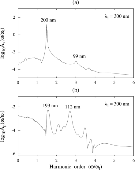
Figure 14: Generation of higher-order harmonics in ${\rm H}_{2}^{+}$ excited by the one-cycle laser pulse at $\lambda_{l}=300$ nm (${\cal E}_{0}=0.045$ au, $\omega_{l}=0.15188$ au, $t_{p}\simeq 1.0$ fs): (a) power spectrum $A_{z}(\omega)$ generated by the optically active $z$ degree of freedom; (b) power spectrum $A_{\rho}(\omega)$ generated by the optically passive, transversal $\rho$ degree of freedom.

In Figure 14, power spectra $A_{z}(\omega)$ and $A_{\rho}(\omega)$ are presented for the case when ${\rm H}_{2}^{+}$ at the laser wavelength of $\lambda_{l}=300$ nm. Again, as it is seen from Figure 14(a), the strongest harmonic in the $A_{z}$ spectrum generated by the optically active $z$ degree of freedom corresponds to the wavelength of $\lambda\simeq 200$ nm. The other higher-order harmonic in the power spectrum $A_{z}(\omega)$, that corresponding to $\lambda\simeq 99$ nm, is (formally) the third-order harmonic with respect to the laser wavelength of $\lambda_{l}=300$ nm used to excite ${\rm H}_{2}^{+}$. On the other hand, the higher-order harmonic at $\lambda\simeq 99$ nm is the second-order harmonic with respect to the smallest-frequency harmonic at $\lambda\simeq 200$ nm appeared in the $A_{z}(\omega)$ power spectrum. Such a new nomenclature of the harmonic order may often be very suitable, because the smallest-frequency harmonics in all power spectra $A_{z}(\omega)$ generated by the optically-active $z$ degree of freedom analyzed in this section above [see Figures 9(a) through 14(a)] are those corresponding to $\lambda\simeq 200$ nm. The physical reason behind this feature is that $\lambda_{l}\simeq 200$ nm is the most efficient laser wavelength with respect to excitation of ${\rm H}_{2}^{+}$ from the ground state to the energy close to its dissociation threshold by one-cycle and two-cycle laser pulses, see Figure 2.

Since the smallest-frequency harmonics in all power spectra $A_{\rho}(\omega)$ generated by the optically-passive $\rho$ degree of freedom [Figures 9(b) through 14(b)] also correspond to $\lambda_{l}\approx 200$ nm, a new nomenclature of the harmonic order described above for $A_{z}(\omega)$ power spectra can be used to analyze power spectra $A_{\rho}(\omega)$ as well. Indeed, it is seen from Figure 14(b) that the higher-order harmonic with the smallest-frequency is that at $\lambda\simeq 193$ nm, while the higher-order harmonic at $\lambda\simeq 112$ nm is approximately the second-order harmonic with respect to the smallest-frequency one (at $\lambda\simeq 193$ nm) and the third-order harmonic with respect to the laser wavelength of $\lambda_{l}=300$ nm used to excite ${\rm H}_{2}^{+}$. Needless to add that, as usual, harmonic at $\lambda\simeq 193$ nm corresponds to the frequency of $\omega^{\rho}_{1}\approx\omega_{\rm osc}$, while harmonic at $\lambda\simeq 112$ nm corresponds to the doubled frequency of $\rho$-oscillations $\omega^{\rho}_{2}\approx 2\omega_{\rm osc}$, where the oscillation frequency $\omega_{\rm osc}$ corresponds to the wavelength $\lambda_{\rm osc}\approx 200$ nm.

Figure 15: Generation of higher-order harmonics in ${\rm H}_{2}^{+}$ excited by the one-cycle laser pulse at $\lambda_{l}=400$ nm (${\cal E}_{0}=0.056$ au, $\omega_{l}=0.11391$ au, $t_{p}\simeq 1.33$ fs): (a) power spectrum $A_{z}(\omega)$ generated by the optically active $z$ degree of freedom; (b) power spectrum $A_{\rho}(\omega)$ generated by the optically passive, transversal $\rho$ degree of freedom.

Finally, in Figure 15, power spectra $A_{z}(\omega)$ and $A_{\rho}(\omega)$ are presented for the case when ${\rm H}_{2}^{+}$ is excited by one-cycle laser pulse at the laser wavelength of $\lambda_{l}=400$ nm. In the usual nomenclature of the harmonic order, three sequential peaks appeared in the power spectrum $A_{z}(\omega)$, Figure 15(a), correspond respectively to the second, the fourth and the fifth harmonics with respect to the laser wavelength of $\lambda_{l}=400$ nm used to excite ${\rm H}_{2}^{+}$. In a suggested new nomenclature, the second and the third peaks (those at 98 and 82 nm) approximately correspond to the second harmonic of the smallest-frequency peak at 200 nm.

In the power spectrum $A_{\rho}(\omega)$, Figure 15(b), the peak at 190 nm corresponds to the second and that at 110 nm approximately corresponds to the fourth harmonic with respect to the laser wavelength of $\lambda_{l}=400$ nm used. On the other hand, the peak at 110 nm approximately corresponds to the second harmonic of the smallest-frequency peak at 190 nm. Again, the peak at 190 nm corresponds to the frequency of $\omega^{\rho}_{1}\approx\omega_{\rm osc}$, while the peak at 110 nm corresponds to the doubled frequency of $\rho$-oscillations $\omega^{\rho}_{2}\approx 2\omega_{\rm osc}$.

4 Conclusion

In the present work, the non-Born-Oppenheimer quantum dynamics of ${\rm H}_{2}^{+}$ excited by linearly polarized along the molecular axis shaped one-cycle laser pulses has been numerically studied at different laser-carrier frequencies corresponding to the laser wavelengths of $\lambda_{l}=$25, 50, 100, 200, 300 and 400 nm. The amplitudes of the one-cycles laser pulses have been optimized such that the energy of ${\rm H}_{2}^{+}$ at the end of each pulse, $\langle E\rangle\simeq-0.515$ au, was close from the below to its dissociation threshold. For the sake of completeness, some results were obtained by making use of two-cycle laser pulses as well. The present work provides a detailed and in-depth extension of our previous study [3] where shaped two-cycle laser pulses at the laser wavelengths of $\lambda_{l}=$800 and 200 nm were used to excite ${\rm H}_{2}^{+}$ close to its dissociation threshold.

The basic results obtained in the present work are summarized as follows.

(I) The most efficient excitation of ${\rm H}_{2}^{+}$ by one-cycle shaped laser pulses, which requires the minimum laser electric-field amplitude to achieve the required energy of about -0.515 au at the end of the pulse, takes place at the laser wavelength of $\lambda_{l}^{\rm opt}\simeq 200$ nm corresponding to the laser-carrier frequency of $\omega_{l}^{\rm opt}\simeq 0.2278$ au. This frequency plays the role of a characteristic oscillation frequency $\omega_{\rm osc}\simeq 0.2278$ au and manifests itself as the carrier frequency of temporally shaped post-laser-field oscillations of the time-dependent expectation values $\langle z\rangle$ and $\langle\partial V/\partial z\rangle$ corresponding to the optically active $z$ degree of freedom, which exist on a long timescale of at least 50 fs after the ends of the pulses used to excite ${\rm H}_{2}^{+}$ initially. The corresponding values for ${\rm H}_{2}^{+}$ excited by two-cycle shaped laser pulses [3] are almost identical.

(II) The optically passive, transversal $\rho$ degree of freedom, which is excited only due to the wave properties of the electron, also demonstrates post-laser-field oscillations of the time-dependent expectation values $\langle\rho\rangle$ and $\langle\partial V/\partial\rho\rangle$ which occur at two basic frequencies $\omega^{\rho}_{1}\approx\omega_{\rm osc}$ and $\omega^{\rho}_{2}\approx 2\omega_{\rm osc}$. The latter frequency corresponds to the frequency-doubling of electronic $\rho$-oscillations as compared to electronic $z$-oscillations described previously [8, 9, 3].

(III) A characteristic feature of power spectra generated by $z$ and $\rho$ degrees of freedom when ${\rm H}_{2}^{+}$ is excited by one-cycle laser pulses is a small number of generated harmonics: not more than three relatively strong harmonics can be observed in the power spectra presented in Section 3.3. A similar feature was observed in the case when ${\rm H}_{2}^{+}$ was excited by two-cycle laser pulses [3]. In a more general case, the number of generated harmonics correlates with the number of optical cycles used to excite a molecule, with the overall trend being “the smaller optical cycles used to excite a molecule is, the smaller number of harmonics is generated”. Such a correlation was discussed in more detail in our previous work [3] for both ordinary (electronic) and muonic molecules.

(IV) The positions of many peaks in power spectra presented in Section 3.3 are not equal to integer multiples of the laser carrier frequency $\omega_{l}$, especially in the case of lower-order harmonic generation at $\lambda_{l}<\lambda_{l}^{\rm opt}\simeq 200$ nm described in Section 3.3.1. It is known [5] that such harmonics may be be generated by single atoms and molecules due to resonance effects. In the current case of one-cycle laser pulses used to excite ${\rm H}_{2}^{+}$ close to its dissociation threshold and the resonant properties of this process depicted in Figure 2, the situation can be rationalized by introducing the suggested above new nomenclature of the harmonic order $\omega/\omega_{l}$ as follows. Since the smallest-frequency harmonics in all power spectra $A_{z}(\omega)$ and $A_{\rho}(\omega)$ presented in Section 3.3 correspond to the optimal wavelength $\lambda_{l}^{\rm opt}\simeq 200$ nm, a new harmonic order $(\omega/\omega_{l})^{\prime}$ can be defined as follows:

$$\left(\frac{\omega}{\omega_{l}}\right)^{\prime}=\left(\frac{\omega}{\omega_{l}}\right)\frac{\lambda_{l}^{\rm opt}}{\lambda_{l}}.$$ (11)

It is easy to check that Equation (11) works very well for all power spectra $A_{z}(\omega)$ and is also quite suitable for power spectra $A_{\rho}(\omega)$ where the frequencies of strongest harmonics are given by $\omega^{\rho}_{1}\approx\omega_{\rm osc}$ and $\omega^{\rho}_{2}\approx 2\omega_{\rm osc}$.

References

- [1] T. Bredtmann, S. Chelkowski and A.D. Bandrauk, J. Phys. Chem. A 116, 11398 (2012).
- [2] A.D. Bandrauk and G.K. Paramonov, Int. J. Mod. Phys. E 23, 1430014 (2014).
- [3] G.K. Paramonov, O. Kühn and A.D. Bandrauk, J. Phys. Chem. A 120, 3175 (2016).
- [4] P.B. Corkum, Phys. Rev. Lett. 71, 1994 (1993).
- [5] T. Kreibich, M. Lein, Y. Engel and E.K.U. Gross, Phys. Rev. Lett. 87, 103901 (2001).
- [6] A. Carrington, I. R. McNab and C. A. Montgomerie, J. Phys. B: At. Mol. Opt. Phys. 22, 3551 (1989).
- [7] I. Kawata, H. Kono, and Y. Fujimura, J. Chem. Phys. 110, 11152 (1999).
- [8] G.K. Paramonov, Chem. Phys. Lett. 411, 350 (2005).
- [9] G.K. Paramonov, Chem. Phys. 338, 329 (2007).
- [10] G.K. Paramonov and P. Saalfrank, Phys. Rev. A 79, 013415 (2009).
- [11] S. Chelkowski and A.D. Bandrauk, Phys. Rev. A 65, 061802 (2002).
- [12] M. Kaluža, J.T. Muckerman, P. Gross, and H.Rabitz, J. Chem. Phys. 100, 4211 (1994).
- [13] H. Kono, Y. Sato, N. Tanaka, T. Kato, K. Nakai, S. Koseki, and Y. Fujimura, Chem. Phys. 304, 203 (2004).
- [14] G.K. Paramonov, O. Kühn and A.D. Bandrauk, Phys. Rev. A 83, 013418 (2011).
- [15] G.K. Paramonov and O. Kühn, J. Phys. Chem. A 116, 11388 (2012).