A Fast 3D Poisson Solver with Longitudinal Periodic and Transverse Open Boundary Conditions for Space-Charge Simulations

Abstract

A three-dimensional (3D) Poisson solver with longitudinal periodic and transverse open boundary conditions can have important applications in beam physics of particle accelerators. In this paper, we present a fast efficient method to solve the Poisson equation using a spectral finite-difference method. This method uses a computational domain that contains the charged particle beam only and has a computational complexity of $O(N_{u}(logN_{mode}))$, where $N_{u}$ is the total number of unknowns and $N_{mode}$ is the maximum number of longitudinal or azimuthal modes. This saves both the computational time and the memory usage by using an artificial boundary condition in a large extended computational domain.

I Introduction

The particle accelerator as one of the most important inventions of the twenty century has many applications in science and industry. In accelerators, a train of charged particle (e.g. proton or electron) beam bunches are transported and accelerated to high energy for different applications. To study the dynamics of those charged particles self-consistently inside the accelerator, the particle-in-cell (PIC) model is usually employed in simulation codes (e.g. the WARP and the IMPACT code suite friedman ; qiang1 ; impact-t ). This PIC model includes both the space-charge forces from the Coulomb interactions among the charged particles within the bunch and the forces from external accelerating and focusing fields at each time step. To calculate the space-charge forces, one needs to solve the Poisson equation for a given charge density distribution. A key issue in the PIC simulation is to solve the Poisson equation efficiently, at each time step, subject to appropriate boundary conditions.

Solving the 3D Poisson equation for the electric potential of a charged beam bunch with longitudinal periodic and transverse open boundary conditions can have important applications in beam dynamics study of particle accelerators. In the accelerator, a train of charged particle bunches as shown in Fig. 1 are produced, accelerated, and transported. If the separation between two bunches is large, each bunch can be treated as an isolated bunch, and the 3D open boundary conditions can be used to solve the Poisson equation. In some accelerators such as a Radio-Frequency Quadrupole (RFQ), the separation between particle bunches is short, to model a single bunch, one needs to use the longitudinal periodic boundary condition rfq . The same model can be used to study space-charge effects in a longitudinally modulated electron beam, where the electron beam density varies periodically from the interaction with the laser beam and the magnetic optic elements dohlus .

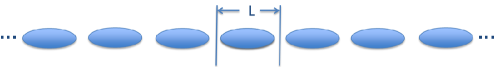
Figure 1: A schematic plot of a train of charged particle beam bunches in the particle accelerator.

In previous studies, a number of methods for solving 3D Poisson’s equation subject to a variety of boundary conditions have been studied haidvogel ; ohring ; hockney ; dang ; braverman ; plagne ; qiang2 ; qiang3 ; lai ; peter ; xu ; rob ; mads ; zheng ; qiang4 ; anderson . However, none of these methods handles the Poisson equation with the longitudinal periodic and transverse open boundary conditions. In the code of reference qiang1 , an image charge method is used to add the contributions from longitudinally periodic bunches into the single bunch’s Green function. Then an FFT method is used to effectively calculate the discrete convolution between the charge density and the new Green’s function that includes contributions from other bunches. The computational cost of this method scales as $O(Nlog(N))$. However, this method requires the computation of the Green’s function from multiple bunch summation. It is not clear, how many bunches are needed in order to accurately emulate the longitudinal periodic boundary condition. In reference dohlus , the image charge method is used with special function to approximate the summation of the Green’s function in different regimes. In practical application, one may not know beforehand what regime should be used for a good approximation. Besides the complexity of the new Green’s function in the image charge method, to use the FFT to calculate the discrete convolution, one needs to double the computational domain with zero padding hockney ; nr . This increases both the computational time and the memory usage.

In this paper, we propose a fast efficient method to solve the 3D Poisson equation with the longitudinal periodic and transverse open boundary conditions. We use a Galerkin spectral Fourier method to approximate the electric potential and the charge density function in the longitudinal and azimuthal dimensions where periodic boundary conditions are satisfied. We then use a second order finite-difference method to solve the radial ordinary differential equation for each mode subject to the transverse open boundary condition. Instead of using a large radial domain with empty space and artificial finite Dirichlet boundary condition to approximate the open boundary condition, we use a domain that contains only the charged particle beam and a boundary matching condition to close the group of linear algebraic equations for each mode. This group of tridiagonal linear algebraic equations can be solved efficiently using the direct Gaussian elimination with a computational cost $O(N)$, where $N$ is the number of unknowns on the radial grid.

The organization of this paper is as follows: After the introduction, we describe the proposed spectral finite-difference numerical method in Section II. Several numerical tests of the 3D Poisson solver are presented in Section III. The conclusions are drawn in Section IV.

II Numerical Methods

The three dimensional Poisson equation in cylindric coordinates can be written as:

$$\frac{\partial^{2}\phi}{\partial r^{2}}+\frac{1}{r}\frac{\partial\phi}{\partial r}+\frac{1}{r^{2}}\frac{\partial^{2}\phi}{\partial\theta^{2}}+\frac{\partial^{2}\phi}{\partial z^{2}}=-\rho(r,\theta,z)$$ (1)

where $\phi$ denotes the electric potential, $\rho$ the charge density function, $r$ and $z$ the radial and longitudinal distance. The longitudinal periodic and transverse open boundary conditions for the potential are:

$$\phi(r=\infty,\theta,z) = 0$$ (2)

$$\phi(r,\theta+2\pi,z) = \phi(r,\theta,z)$$ (3)

$$\phi(r,\theta,z+L) = \phi(r,\theta,z)$$ (4)

Given the periodic boundary conditions of the electric potential along the $\theta$ and the $z$, we use a Galerkin spectral method with the Fourier basis function to approximate the charge density function $\rho$ and the electric potential $\phi$ along these two dimensions as:

$$\rho(r,\theta,z) = \sum_{n=-N_{n}/2}^{n=N_{n}/2-1}\sum_{m=-N_{m}/2}^{m=N_{m}/2-1}\rho_{n}^{m}(r)\exp(-ia_{n}z)\exp(-im\theta)$$ (5)

$$\phi(r,\theta,z) = \sum_{n=-N_{n}/2}^{n=N_{n}/2-1}\sum_{m=-N_{m}/2}^{m=N_{m}/2-1}\phi_{n}^{m}(r)\exp(-ia_{n}z)\exp(-im\theta)$$ (6)

where

$$\rho_{n}^{m}(r) = \frac{2}{L\pi}\int_{0}^{L}\int_{0}^{2\pi}\rho(r,\theta,z)\exp(im\theta)\exp(ia_{n}z)\ d\theta dz$$ (7)

$$\phi_{n}^{m}(r) = \frac{2}{L\pi}\int_{0}^{L}\int_{0}^{2\pi}\phi(r,\theta,z)\exp(im\theta)\exp(ia_{n}z)\ d\theta dz$$ (8)

and $a_{n}=n2\pi/L$, $L$ is the longitudinal periodic length. Substituting the above expansions into the Poisson Eq. 1 and making use of the orthonormal condition of the Fourier function, we obtain:

$$\frac{\partial^{2}\phi^{m}_{n}}{\partial r^{2}}+\frac{1}{r}\frac{\partial\phi_{n}^{m}}{\partial r}-(\frac{m^{2}}{r^{2}}+(a_{n})^{2})\phi_{n}^{m} = -{\rho_{n}^{m}}$$ (9)

This is a group of decoupled ordinary differential equations that can be solved for each individual mode $m$ and $n$. For these equations, at $r=0$, we have the boundary conditions:

$$\frac{\partial\phi_{n}^{m}}{\partial r}(0) = 0;\ \ for\ \ m=0$$ (10)

$$\phi_{n}^{m}(0) = 0;\ \ for\ \ m\neq 0$$ (11)

Assuming all charged particles within the beam bunch are contained within a radius $R$, we discretize the above equation using a second order finite-difference scheme, and obtain a group of linear algebraic equations for each mode $(m,n)$ as:

$$(\frac{r_{i}^{2}}{h^{2}}-\frac{r_{i}}{2h})\phi_{n}^{m}(r_{i-1})-(\frac{2r_{i}^{2}}{h^{2}}+m^{2}+a_{n}^{2}r_{i}^{2})\phi_{n}^{m}(r_{i})+(\frac{r_{i}^{2}}{h^{2}}+\frac{r_{i}}{2h})\phi_{n}^{m}(r_{i+1})=-r_{i}^{2}{\rho_{n}^{m}(r_{i})}$$ (12)

where $i=1,2,\cdots,N$, and $r_{i}=ih$. The boundary conditions at $r=0$ are approximated as:

$$-\frac{3}{2}\phi_{n}^{m}(r_{0})+2\phi_{n}^{m}(r_{1})-\frac{1}{2}\phi_{n}^{m}(r_{2}) = 0;\ \ for\ \ m=0$$ (13)

$$\phi_{n}^{m}(r_{0}) = 0;\ \ for\ \ m\neq 0$$ (14)

For $m=0$, there are only $N+1$ linear equations but $N+2$ unknowns, and for $m\neq 0$, there are only $N$ linear equations but $N+1$ unknowns. For the potential outside the radius $R$, the Eq. 9 can be written as:

$$\frac{\partial^{2}\phi^{m}_{n}}{\partial r^{2}}+\frac{1}{r}\frac{\partial\phi_{n}^{m}}{\partial r}-(\frac{m^{2}}{r^{2}}+(a_{n})^{2})\phi_{n}^{m} = 0$$ (15)

subject to the open boundary conditions

$$\phi_{n}^{m}(r=\infty) = 0$$ (16)

For $n\neq 0$, a formal solution of the equation 15 subject to the boundary condition 16 can be written as:

$$\phi_{n}^{m}(r) = A\ K_{m}(a_{n}r)$$ (17)

where $K_{m}$ is the second kind modified Bessel function. Using the above equation and the continuity of the potential at $r_{N}$, we obtain another equation for the unknowns $\phi_{n}^{m}(r_{N})$ and $\phi_{n}^{m}(r_{N+1})$ as:

$$\phi_{n}^{m}(r_{N})K_{m}(a_{n}r_{N+1}) = \phi_{n}^{m}(r_{N+1})K_{m}(a_{n}r_{N})$$ (18)

For $n=0$,$m\neq 0$, the Eq. 15 is reduced to the Cauchy-Euler equation:

$$\frac{\partial^{2}\phi^{m}_{0}}{\partial r^{2}}+\frac{1}{r}\frac{\partial\phi_{0}^{m}}{\partial r}-\frac{m^{2}}{r^{2}}\phi_{0}^{m} = 0$$ (19)

A formal solution of this equation that satisfies the open radial boundary condition can be written as:

$$\phi_{0}^{m}(r) = Ar^{-m}$$ (20)

From the above equation, we obtain another equation for the unknowns $\phi_{0}^{m}(r_{N})$ and $\phi_{0}^{m}(r_{N+1})$ as:

$$\phi_{0}^{m}(r_{N})r_{N}^{m} = \phi_{0}^{m}(r_{N+1})r_{N+1}^{m}$$ (21)

For $n=0$,$m=0$, the Eq. 15 is reduced to:

$$\frac{\partial^{2}\phi^{0}_{0}}{\partial r^{2}}+\frac{1}{r}\frac{\partial\phi_{0}^{0}}{\partial r} = 0$$ (22)

A formal solution of this equation that satisfies the open radial boundary condition can be written as:

$$\phi_{0}^{0}(r) = A\log(r)$$ (23)

From this equation, we obtain another equation for the unknowns $\phi_{0}^{0}(r_{N})$ and $\phi_{0}^{0}(r_{N+1})$ as:

$$\phi_{0}^{0}(r_{N})\log(r_{N+1}) = \phi_{0}^{0}(r_{N+1})\log(r_{N})$$ (24)

Using Eqs. 18, 21, 24, we have $N+2$ linear equations for $N+2$ unknowns for $m=0$ and $N+1$ linear equations for $N+1$ unknowns for $m\neq 0$. For each mode $m$ and $n$, this is a group of tridiagonal linear algebraic equations, which can be solved effectively using direct Gaussian elimination with the number of operations scaling as $O(N)$. Since both Fourier expansions in $\theta$ and $z$ can be computed very effectively using the FFT method, the total computational complexity of the proposed algorithm scales as $O(NN_{m}N_{n}log(N_{m}N_{n}))$.

III Numerical Tests

The numerical algorithm discussed in the preceding section is tested using two charge density distribution functions. The first example is an infinite long cylindric coasting beam with uniform charge distribution within the radius $R=2$. The charge density function is given as

$$\rho(r,\theta,z) = \left\{\begin{array}[]{r@{\quad:\quad}l}1.0&r\leq 2\\ 0.0&r>2\end{array}\right.$$ (27)

For this charge density function, there is only the radial component of the electric field. The analytical solution of the electric field can be found as:

$$E_{r}(r) = \frac{r}{2}\ \ for\ r\leq 2$$ (28)

Figure 2 shows the longitudinal electric field and the transverse radial electric field from the numerical solution and the above analytical solution. It is seen that the numerical solution agrees with the analytical solution very well.

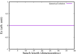
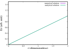
Figure 2: Longitudinal electric field profile Ez on the z-axis (left) and the transverse radial electric field profile Er in the middle of the bunch from the numerical solutions together with the analytical solution (right) in a uniform cylinder coasting beam.

In the second test example, we assume that there is a longitudinal modulation of the charged particle density distribution. The charge density function is given as:

$$\rho(r,\theta,z) = \left\{\begin{array}[]{r@{\quad:\quad}l}4-4(r/R)^{2}+\sin(a_{1}z)[4-(a_{1}r)^{2}]/5&r\leq R\\ 0.0&r>R\end{array}\right.$$ (31)

The analytical solution of the electric fields for this charge distribution can be written as:

$$E_{z}(r,z) = a_{1}\cos(a_{1}z)[r^{2}-AI_{0}(a_{1}r)]/5$$ (32)

$$E_{r}(r,z) = 2r-r^{3}/R^{2}+\sin(a_{1}z)[2r-Aa_{1}I_{1}(a_{1}r)]/5$$ (33)

where the constant $A$ is given as:

$$A = \frac{R^{2}a_{1}K_{1}(a_{1}R)+2RK_{0}(a_{1}R)}{a_{1}I_{1}(a_{1}R)K_{0}(a_{1}R)+a_{1}I_{0}(a_{1}R)K_{1}(a_{1}R)}$$ (34)

Here, the matching condition at the edge $R$ is used together with the analytical formal solution Eq. 17 for the open boundary condition to determine the above constant $A$. Figure 3 shows the longitudinal electric field and the transverse radial electrical field from the numerical solutions and from the analytical solutions. The numerical solutions and the analytical solutions agree with each other very well in this longitudinally modulated charged particle beam too. Here, we have assumed $R=10$ and $L=\pi R$.

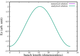
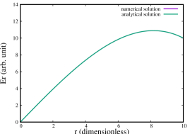
Figure 3: Longitudinal electric field profile Ez on the z-axis (left) and the transverse radial electric field profile Er in the middle of the bunch (right) from the numerical solutions together with the analytical solutions in a longitudinally modulated charged particle beam bunch.

The numerical method proposed in the preceding section has the advantage that uses a computational domain that contains the charged particle beam only while satisfying the transverse open boundary condition. In principle, the transverse open boundary can be approximated by an artificial closed Dirichlet boundary condition in a larger computational domain. Since only the electric fields inside the charge particle beam bunch are needed in the self-consistent accelerator space-charge beam dynamics simulation, this larger computational domain by using the artificial Dirichlet boundary condition will waste both the computational time and the memory storage in the empty computational domain. In the following, we use a simplified one-dimensional equation from above equations to illustrate the advantage of the above proposed method.

For $m=0$ and $n=1$, Eq. 9 is reduced to:

$$\frac{\partial^{2}\phi^{0}_{1}}{\partial r^{2}}+\frac{1}{r}\frac{\partial\phi_{1}^{0}}{\partial r}-a_{1}^{2}\phi_{1}^{0} = -\rho_{1}^{0}$$ (35)

Assuming a radial charge distribution $\rho_{1}^{0}(r)$ as:

$$\rho_{1}^{0}(r) = \left\{\begin{array}[]{r@{\quad:\quad}l}4-(a_{1}r)^{2}&r\leq R\\ 0.0&r>R\end{array}\right.$$ (38)

we can have an analytical solution as:

$$\phi^{0}_{1}(r) = -r^{2}+AI_{0}(a_{1}r)$$ (39)

where the constant $A$ is given in Eq. 34. Figure 4 shows the electric potential and the relative errors as a function of radial distance from the analytical solution, and from the proposed numerical solution with transverse open boundary condition ($R=10$), from the artificial transverse closed Dirichlet boundary condition using two times computational domain ($\phi_{1}^{0}(R=20)=0$), and from the artificial transverse closed boundary condition using four times computational domain ($\phi_{1}^{0}(R=40)=0$).

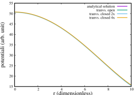
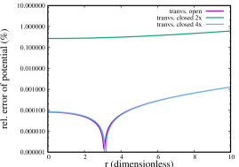
Figure 4: The electric potential (left) and the relative errors (right) from the analytical solution and from the numerical solution with transverse open, transverse closed with two times radial computational domain, and transverse closed with four times computational domain.

It is seen that even using two times computational domain, the artificial closed boundary condition solution still shows much larger errors than the proposed open boundary numerical solution. It appears that four times larger computational domain is needed in the artificial closed boundary solution in order to attain the same numerical accuracy as the open boundary solution that uses a domain with radius $R$ that contains the charged particle beam only. In the above example, we have used $201$ radial grid points for the open boundary solution, $401$ grid points for the artificial closed boundary solution with two times computational domain and $801$ grid points for the solution with four times computational domain.

IV Conclusions

In this paper, we presented a fast three-dimensional Poisson solver subject to longitudinal periodic and transverse open boundary conditions. Instead of using a larger artificial computational domain with closed Dirichlet boundary condition, this solver uses a computational domain that contains the charged particles only. This saves both the computational time and the memory usage compared with the artificial closed boundary condition method. By using the FFT method to calculate the longitudinal and azimuthal Fourier expansion and the direct Gaussian elimination to solve the radial tridiagonal linear algebraic equations, the computational complexity of the proposed numerical method scales as $O(N_{u}(logN_{mode}))$. This makes this fast Poisson solver very efficient and can be included in the self-consistent space-charge simulation PIC codes for space-charge beam physics study in particle accelerators.

V ACKNOWLEDGEMENTS

This work was supported by the U.S. Department of Energy under Contract No. DE-AC02-05CH11231. This research used computer resources at the National Energy Research Scientific Computing Center.

References

- (1) A. Friedman, D. P. Grote and I. Haber, Phys. Fluids B 4, 2203 (1992). pp. 156-158.
- (2) J. Qiang, R. D. Ryne, S. Habib, V. Decyk, J. Comput. Phys. 163, 434 (2000).
- (3) J. Qiang, S. Lidia, R. D. Ryne, and C. Limborg-Deprey, Phys. Rev. ST Accel. Beams 9, 044204, 2006.
- (4) R. Duperrier, Phys. Rev. ST Accel. Beams 3, 124201, 2000.
- (5) M. Dohlus and Ch. Henning, Phys. Rev. Accel. Beams 19, 034401 (2016).
- (6) D. B. Haidvogel and T. Zang, J. Comput. Phys. 30, 167 (1979).
- (7) S. Ohring, J. Comput. Phys. 50, 307 (1983).
- (8) R.W. Hockney, J.W. Eastwood, Computer Simulation Using Particles, Adam Hilger, New York, 1988.
- (9) H. Dang-Vu and C. Delcarte, J. Comput. Phys. 104, 211 (1993).
- (10) E. Braverman, M. Israeli, A. Averbuch, and L. Vozovoi, J. Comput. Phys. 144, (1998).
- (11) L. Plagne and J. Berthou, J. Comput. Phys. 157, 419 (2000).
- (12) J. Qiang and R. D. Ryne, Comp. Phys. Comm. 138, 18 (2001).
- (13) J. Qiang and R. Gluckstern, Comp. Phys. Comm. 160, 120, (2004).
- (14) M. Lai, Z. Li, X. Lin, J. Comp. Appl. Math. 191, 106, (2006).
- (15) P. McCorquodale, P. Colella, G. T. Balls, and S. B. Baden, Comm. App. Math. and Comp. Sci. 2, 57, (2007).
- (16) J. Xu, P. N. Ostroumov, J. Nolen, Comp. Phys. Comm. 178, 290 (2008).
- (17) R. D. Ryne, ”On FFT based convolutions and correlations, with application to solving Poisson’s equation in an open rectangular pipe,” arXiv:1111.4971v1, 2011.
- (18) M. M. Hejlesen, J. T. Rasmussen, P. Chatelain, J. H. Walther, J. Comput. Phys. 252, 458 (2013).
- (19) D. Zheng, G. Poplau, and U. van Rienen, Comp. Phys. Comm. 198, 82 (2016).
- (20) J. Qiang, Comp. Phys. Comm. 203, 122, (2016).
- (21) C. R. Anderson, J. Comput. Phys. 314, 194 (2016).
- (22) W.H. Press, B.P. Flannery, S.A. Teukolsky, W.T. Vetterling, Numerical Recipes in FORTRAN: The Art of Scientific Computing, 2nd ed., Cambridge University Press, Cambridge, England, 1992.