Influence of a Pseudo Aharonov-Bohm field on the quantum Hall effect in Graphene

Abstract

The effect of an Aharonov-Bohm (AB) pseudo magnetic field on a two dimensional electron gas in graphene is investigated. We consider it modeled as in the usual AB effect but since such pseudo field is supposed to be induced by elastic deformations, the quantization of the field flux is abandoned. For certain constraints on the orbital angular momentum eigenvalues allowed for the system, we can observe the zero Landau level failing to develop, due to the degeneracy related to the Dirac valleys $K$ and $K^{\prime}$ which is broken. For integer values of the pseudo AB flux, the actual quantum Hall effect is preserved. Obtaining the Hall conductivity by summing over all orbital angular momentum eigenvalues, the zero Landau levels is recovered. Since our problem is closed related to the case where topological defects on a graphene sheet are present, the questions posed here are helpful if one is interested to probe the effects of a singular curvature in these systems.

1 Introduction

The study of quantum dynamics for particles in constant magnetic [1] and Aharonov-Bohm (AB) flux fields [2], which are perpendicular to the plane where the particles are confined, has been carried out over the last years. The existence of other potentials are also included, depending on the purpose of the investigation. For example, in Ref. [3] an exactly soluble model to describe quantum dots, antidots, one-dimensional rings and straight two-dimensional wires in the presence of such fields was proposed. It is an ideal tool to investigate the AB effects and the persistent currents in quantum rings, for instance. In Ref. [4], the exact bound-state energy eigenvalues and the corresponding eigenfunctions for several diatomic molecular systems in a pseudoharmonic potential were analytically calculated for any arbitrary angular momentum. The Dirac bound states of anharmonic oscillator under external magnetic and AB flux fields were addressed recently [5]. The investigation of a Cornell Potential in external fields was considered in Ref. [6]. Other examples can be found elsewhere. It would be interesting to carry out such investigations on graphene, an one atom thick material which rapidly caught the attention of many physicists [7]. Graphene, a single layer of carbon atoms in a honeycomb lattice, is considered a truly two dimensional system. The carriers within it behave as two-dimensional massless Dirac fermions [8]. Due to its peculiar physical properties, graphene has great potential for nanoelectronic applications [9, 10, 11]. Graphene can be considered a zero-gap semiconductor. This fact prevent the pinch off of charge currents in electronic devices. Quantum confinement of electrons and holes in nanoribbons [12] and quantum dots [13] can be realized in order to induce a gap. However, this lattice disorder suppress an efficient charge transport [14]. One alternative to open a gap is to induce a strain field in a graphene sheet onto appropriate substrates [14]. They play the role of an effective gauge field which yields a pseudo magnetic field [15]. Unlike actual magnetic fields, these strain induced pseudo magnetic fields do not violate the time reversal symmetry [16]. A numerical study on the uniformity of the pseudomagnetic field in graphene as the relative orientation between the graphene lattice and straining directions was carried out in Ref. [17] and it was observed that observing the pseudomagnetic field in Raman spectroscopy setup is feasible. In Ref. [18], two different mechanisms that could underlie nanometer-scale strain variations in graphene as a function of externally applied tensile strain is presented.

Recently, some works devoted to the search for solutions of the Dirac equation with position dependent magnetic fields were addressed in this context [19, 20, 21, 22, 23]. However, they consider actual instead of pseudo magnetic fields. No experiments have been reported yet and we believe it is because such field configurations are not easy to implement in the laboratory. In this paper, we investigate a graphene sheet in the presence of both a constant orthogonal magnetic and a pseudo Aharonov-Bohm field. This kind of pseudo AB field was first investigated in [24], where a device to detect microstresses in graphene able to measure AB interferences at the nanometer scale was proposed. It was showed on it that fictitious magnetic field associated with elastic deformations of the sample yield interferences in the local density of states. Here, we consider such pseudo AB-field modeled like a “thin solenoid” so we can analytically investigate the consequences in the Quantum Hall effect, for instance. Specifically, we investigate how such non constant pseudo AB field modify the relativistic Landau levels and, as consequence, the Hall conductivity in a suspended graphene. Since such pseudo AB field is modeled as the actual AB field, which is yielded by a thin tube flux, either regular or irregular wavefunctions can be solution of the problem. This is in agreement with other quantum problems where singularities have also appeared. This question about the correct behavior of wavefuntion whenever we have singularities has been investigated via the self adjoint extension approach over the last years [25, 26, 27, 28, 29, 30] . In our case, if singular effects manifest, then a constraint in the orbital angular momentum eigenvalues appears.

An important result is that, for certain constraints on the orbital angular momentum eigenvalues allowed for the system, the zero-energy, which exist in the known relativistic Landau levels when just the constant orthogonal magnetic field is present, does not develop around both valleys, $K$ and $K^{\prime}$. The consequence is that a Hall plateau develop at the null filling factor (dimensionless ratio between the number of charge carries and the flux quanta). This is due to the degeneracy related to the Dirac valleys $K$ and $K^{\prime}$ which is broken. For the integer values of the AB flux, the zero energy manifests again around both valleys. On the other hand, by analyzing the quantum Hall conductivity summing for all the orbital angular momentum eigenvalues allowed for the system, we observe that the standard plateaux at all integer $n$ of $2e^{2}/h$ will show up, including that for $n=0$. This is also due to the degeneracy related to the Dirac valleys $K$ and $K^{\prime}$ which is broken for certain part of the energy spectrum. This is in contrast to the usual Quantum Hall effect in graphene, where the quantum Hall conductivity exhibits the standard plateaux at all integer $n$ of $4e^{2}/h$, for $n=1,2,3..$, and $2e^{2}/h$ for $n=0$.

The plan of this work is the following. First, we investigate how a varying pseudo magnetic field perpendicular to a graphene sheet is going to affect the relativistic Landau levels. Then, we investigate the influence of such pseudo AB field in the quantized Hall conductivity. At the end, we have the concluding remarks.

2 Modifications in the Relativistic Landau Levels under pseudo-AB field

In this section, we will investigate how a pseudo AB field is going to affect the relativistic Landau levels. First, we must remember the reader that the low energy excitations of graphene behave as massless Dirac fermions, instead of massive electrons. Their internal degrees of freedom are: sublattice index (pseudospin), valley index (flavor) and real spin, each taking two values. The real spin is irrelevant in our problem and will not be taken into account, except for an additional degeneracy factor $2$ in the Hall conductivity. Then, the low energy excitations around a valley is described by the $(2+1)-$dimensional Dirac equation as

$$-i\hbar v_{F}\left(\mathbf{\sigma}\cdot\mathbf{\nabla}\right)\Psi(\mathbf{r})=E\Psi(\mathbf{r}),$$ (1)

where $\sigma=\left(\sigma_{x},\sigma_{y}\right)$ are the Pauli matrices, $\Psi=(\varphi_{1},\varphi_{2})^{T}$ is a two component spinor field, the speed of light $c$ was replaced by the Fermi velocity ($v_{F}\approx 10^{6}$m/s) and $\hbar$ has been fixed equal to one. The electronic states around the zero energy are states belonging to distinct sublattices. This is the reason we have a two component wavefunction. Two indexes to indicate these sublattices, similar to spin indexes (up and down), must be used. The inequivalent corners of the Brillouin zone, which are called Dirac points, are labeled as $K$ and $K^{{}^{\prime}}$(valley index) [8]. In what follows, we consider $v_{F}=\hbar=1$. We reinstate the proper units latter, in the analysis of our main results.

In this work, the pseudo varying magnetic field is supposed to appear due strains on a graphene sheet [15]. The valleys $K$ and $K^{{}^{\prime}}$ feel an effective field of $\tilde{\mathbf{A}}\pm\mathbf{A}$, where $\tilde{\mathbf{A}}$ is due to a real magnetic field and $\mathbf{A}$ is due to a pseudo-magnetic field. Notice that a different sign has to be used for the gauge field due to strain at the valleys $K$ and $K^{{}^{\prime}}$ since such fields do not break time reversal symmetry [16]. These vector potentials can be inserted into the Dirac equation via a minimal coupling, $\mathbf{p}\rightarrow\mathbf{p}-e\mathbf{A}$. We begin by writing the massless Dirac equation for the four-component spinor $\Psi$

$$\left[\beta\mathbf{\gamma}\cdot\left(\mathbf{p}-e\mathbf{A}\right)-E\right]\Psi\left(\mathbf{r}\right)=0,$$ (2)

with the $\beta,\mathbf{\gamma}$ matrices being given in terms of the Pauli matrices as [31]

$$\beta=\sigma^{z},\qquad\beta\gamma^{1}=\sigma^{1},\qquad\beta\gamma^{2}=s\sigma^{2},$$ (3)

where the parameter $s$, which has a value of twice the spin value, can be introduced to characterizing the two pseudo spin states, with $s=+1$ for spin “up” and $s=-1$ for spin “down”. Equation (2) can be placed on a quadratic form by applying the operator $E+\beta\mathbf{\gamma}\cdot\left(\mathbf{p}-e\mathbf{A}\right)$. The result of this application provides the Dirac-Pauli equation

$$\left[\mathbf{p}^{2}-2e\left(\mathbf{A}\cdot\mathbf{p}\right)+e^{2}\mathbf{A}^{2}-es\hbar\left(\mathbf{\sigma}\cdot\mathbf{B}\right)\right]\psi\left(\mathbf{r}\right)=E^{2}\psi\left(\mathbf{r}\right),$$ (4)

where $\psi\left(\mathbf{r}\right)$ is a a four-component spinorial wave function. We consider the case where the particle interacts with a gauge field

$$\mathbf{A=A}_{1}+\mathbf{A}_{2},$$ (5)

with

$$\mathbf{A}_{1}=\frac{B_{0}r}{2}\mathbf{\hat{\varphi}},\leavevmode\nobreak\ \leavevmode\nobreak\ \leavevmode\nobreak\ \mathbf{A}_{2}=\frac{\phi}{r}\mathbf{\hat{\varphi}},$$ (6)

where $B$ is the magnetic field magnitude and $\phi$ is the flux parameter. The potentials in Eq. (5) both provide one magnetic field perpendicular to the plane $\left(r,\varphi\right)$, namely

$$\mathbf{B}=\mathbf{B}_{1}+\mathbf{B}_{2},$$ (7)

with

$$\mathbf{B}_{1} = \mathbf{\nabla}\times\mathbf{A}_{1}=B\mathbf{\hat{z}},$$ (8)

$$\mathbf{B}_{2} = \mathbf{\nabla}\times\mathbf{A}_{2}=\phi\frac{\delta\left(r\right)}{r}\mathbf{\hat{z}}.$$ (9)

Note that the field (9) is one produced by a solenoid. If the solenoid is extremely long, the field inside is uniform, and the field outside is zero. But, the vector potential outside the solenoid is not zero. However, in a general dynamics, the particle is allowed to access the $r=0$ region. In this region, the pseudo magnetic field is non-null. If the radius of the solenoid is $r_{0}\approx 0$, then the relevant magnetic field is $\mathbf{B}_{2}\sim\delta\left(r\right)$ as in Eq. (9).

Adopting the decomposition

$$\left(\begin{array}[]{c}\psi_{1}\left(r,\varphi\right)\\ \psi_{2}\left(r,\varphi\right)\end{array}\right)=\left(\begin{array}[]{c}\sum\limits_{m}f_{m}\left(r\right)\;e^{im\varphi}\\ i\sum\limits_{m}g_{m}\left(r\right)\;e^{i(m+s)\varphi}\end{array}\right),$$ (10)

with $m+1/2=\pm 1/2,\pm 3/2,\ldots$, with $m\in\mathbb{Z}$, and inserting this into Eq. (4), the equation for $f_{m}\left(r\right)$ is found to be

$$hf_{m}\left(r\right)=k^{2}f_{m}\left(r\right),$$ (11)

where

$$k^{2}=E^{2}+\left(m+s\right)eB-e^{2}\phi B,$$ (12)

$$h=h_{0}-se\phi\frac{\delta\left(r\right)}{r},$$ (13)

$$h_{0}=-\frac{d^{2}}{dr^{2}}-\frac{1}{r}\frac{d}{dr}+\frac{1}{r^{2}}\left(m-\lambda\right)^{2}+\omega^{2}r^{2},$$ (14)

and $\lambda=e\phi$ and $\omega={eB}/{2}$. Note that Eq. (11) contains the $\delta$ function in the radial Hamiltonian $h$, which is singular at the origin. In order to deal with a Hamiltonian of this nature we making use of the self-adjoint extension approach [32, 33]. According to Ref. [34], the Hamiltonian $h_{0}$ is essentially self-adjoint if $\left|m-\lambda\right|\geq 1$, while for $\left|m-\lambda\right|<1$ it admits an one-parameter family of self-adjoint extensions, $h_{0,\zeta_{m}}$, where $\zeta_{m}$ is the self-adjoint extension parameter. To characterize this family of self-adjoint extensions, we use the approach proposed in [33], which uses the boundary condition at the origin

$$f_{0}=\zeta_{m}f_{1},$$ (15)

with

$$f_{0}={} \lim_{r\rightarrow 0^{+}}r^{|m-\lambda|}f_{m}\left(r\right),$$

$$f_{1}={} \lim_{r\rightarrow 0^{+}}\frac{1}{r^{|m-\lambda|}}\left[f_{m}\left(r\right)-f_{0}\frac{1}{r^{|m-\lambda|}}\right],$$

where $\zeta_{m}\in\mathbb{R}$ is the self-adjoint extension parameter. In the boundary condition above, if $\zeta_{m}=0$, we have the free Hamiltonian (without the $\delta$ function) with regular wave functions at the origin, and for $\zeta_{m}\neq 0$, the boundary condition in Eq. (15) permit an $r^{-\left|m-\lambda\right|}$ singularity in the wave functions at the origin.

3 The bound state energy and wave function

With the application of the boundary condition (15), we can find the energy spectrum of the system. Before doing this, first we make a variable change in Eq. (11), $\rho=\omega r^{2}$, so that it is written as ( $r\neq 0$)

$$\rho\frac{d^{2}f_{m}}{d\rho^{2}}+\frac{df_{m}}{d\rho}-\left[\frac{\left(m-\lambda\right)^{2}}{4\rho}+\frac{\rho}{4}-\frac{k^{2}}{4\omega}\right]f_{m}=0.$$ (16)

Moreover, because of the boundary condition (15), we seek for regular and irregular solutions for Eq. (16). So, after studying the asymptotic limits of Eq. (16), we find the following regular ($+$ ) (irregular ($-$)) solution:

$$f_{m}\left(\rho\right)=\rho^{\pm\frac{1}{2}\left|m-\lambda\right|}e^{-\rho/2}F\left(\rho\right).$$ (17)

Insertion of this solution into Eq. (16) yields

$$\rho F^{\prime\prime}\left(\rho\right)+\left(1\pm\left|m-\lambda\right|-\rho\right)F^{\prime}\left(\rho\right)-\left(\frac{1\pm\left|m-\lambda\right|}{2}-\frac{k^{2}}{4\omega}\right)F\left(\rho\right)=0.$$ (18)

The general solution to this equation is given in terms of the confluent hypergeometric function of the first kind [35],

$$f_{m}\left(\rho\right) =a_{m}\rho^{\frac{1}{2}\left|m-\lambda\right|}e^{-\frac{\rho}{2}}\;F\left(d_{+},1+\left|m-\lambda\right|,\rho\right)$$

$$+b_{m}\rho^{-\frac{1}{2}\left|m-\lambda\right|}e^{-\frac{\rho}{2}}\;F\left(d_{-},1-\left|m-\lambda\right|,\rho\right),$$ (19)

with

$$d_{\pm}=\frac{1\pm\left|m-\lambda\right|}{2}-\frac{k^{2}}{4\omega},$$ (20)

where $a_{m}$ and $b_{m}$ are, respectively, the coefficients of the regular and irregular solutions.

Now, by applying the boundary condition (15), one finds the following relation between the coefficients $a_{m}$ and $b_{m}$

$$\zeta_{m}\omega^{\left|m-\lambda\right|}=\frac{b_{m}}{a_{m}}\left[1+\frac{\zeta_{m}k^{2}}{4\left(1-\left|m-\lambda\right|\right)}\lim_{r\rightarrow 0^{+}}r^{2-2\left|m-\lambda\right|}\right].$$ (21)

Note that $\lim_{r\rightarrow 0^{+}}r^{2-2\left|m-\lambda\right|}$ diverges if $\left|m-\lambda\right|\geq 1$. This condition implies that $b_{m}$ must be zero if $\left|m-\lambda\right|\geq 1$ and only the regular solution contributes to $f_{m}\left(\rho\right)$. For $\left|m-\lambda\right|<1$, when the operator $H_{0}$ is not self-adjoint, there arises a contribution of the irregular solution to $f_{m}\left(r\right)$ [28, 36, 37]. In this manner, the contribution of the irregular solution for the system wave function stems from the fact that the operator $H_{0}$ is not self-adjoint.

For $f_{m}(r)$ be a bound state wave function, it must vanish at large values of $r$, i.e., it must be normalizable. So, from the asymptotic representation of the confluent hypergeometric function, the normalizability condition is translated in

$$\frac{b_{m}}{a_{m}}=-\frac{\Gamma\left(1+\left|m-\lambda\right|\right)}{\Gamma\left(1-\left|m-\lambda\right|\right)}\frac{\Gamma\left(d_{-}\right)}{\Gamma\left(d_{+}\right)}.$$ (22)

From Eq. (21), for $\left|m-\lambda\right|<1$, we have

$$\frac{b_{m}}{a_{m}}=\zeta_{m}\omega^{\left|m-\lambda\right|}.$$ (23)

By combining this result with (22), one finds

$$\frac{\Gamma\left(d_{+}\right)}{\Gamma\left(d_{-}\right)}=-\frac{1}{\zeta_{m}\omega^{\left|m-\lambda\right|}}\frac{\Gamma\left(1+\left|m-\lambda\right|\right)}{\Gamma\left(1-\left|m-\lambda\right|\right)}.$$ (24)

Equation (24) implicitly determines the energy spectrum for different values of the self-adjoint extension parameter. Two limiting values for the self-adjoint extension parameter deserve some attention. For $\zeta_{m}=0$, when the $\delta$ interaction is absent, only the regular solution contributes for the bound state wave function. On the other side, for $\zeta_{m}=\infty$ only the irregular solution contribute for the bound state wave function. For all other values of the self-adjoint extension parameter, both regular and irregular solutions contributes for the bound state wave function. The energies for the limiting values are obtained from the poles of the gamma function, namely,

$$\left\{\begin{array}[]{lll}d_{+}=-n&\mbox{for }\zeta_{m}=0&\mbox{(regular solution)},\\ d_{-}=-n&\mbox{for }\zeta_{m}=\infty&\mbox{(irregular solution)},\end{array}\right.$$ (25)

with $n$ a nonnegative integer, $n=0,1,2,\ldots$. By manipulation of Eq. ( 25), we obtain

$$E^{2}=eB\left[2n+1\pm\left|m-\lambda\right|+\lambda-m-s\right].$$ (26)

In particular, it should be noted that for the case when $\left|m-\lambda\right|\geq 1$ or when the $\delta$ interaction is absent, only the regular solution contributes for the bound state wave function ($b_{m}=0$), and the energy is given by Eq. (26) with plus sign. The energy spectrum above must be analyzed in terms of the values that the parameter $\lambda$ can assume, since the condition $\left|m-\lambda\right|\geq 1$($\left|m-\lambda\right|<1$) for the regular(irregular) solution has to be fulfilled. Let us consider the regular wave functions at first. Then, the spectrum (26) in this case can be written as

$$E_{n}^{+}=\pm\sqrt{2eBn^{\prime}}$$ (27)

for $m-\lambda>1$, with $n^{\prime}=n+\frac{1-s}{2}=0,1,2,3,...$, and

$$E_{n}^{-}=\pm\sqrt{2eB\left(n^{\prime}+\lambda\right)},$$ (28)

for $m-\lambda<-1$, with $n^{\prime}=n+\frac{1-s}{2}-m=0,1,2,3,...$. The energy spectrum around the Dirac point $K^{\prime}$ is obtained by changing $\lambda\rightarrow-\lambda$. This way, we have

$$E_{n}^{+}=\pm\sqrt{2eBn^{\prime}}$$ (29)

for $m-\lambda>1$, with $n^{\prime}=n+\frac{1-s}{2}=0,1,2,3,...$, and

$$E_{n}^{-}=\pm\sqrt{2eB\left(n^{\prime}+1-\lambda\right)}.$$ (30)

for $m-\lambda<-1$, with $n^{\prime}=n+\frac{1-s}{2}-m=0,1,2,3,...$. If we had chosen $\lambda<0$ at first, the results above are the same, but exchanged between $K^{\prime}$ and $K$. If $\lambda$ is integer, the energy spectrum of the system will be the same as in the case without such AB field, $E_{n}^{-}=\pm\sqrt{2eBn}$, since $n=n^{\prime}\pm\lambda=0,1,2,3,...$. In this case, the parameter $\lambda$ does not splits the energy levels and the degeneracy regardless the Dirac valleys is not broken.

We now turn our attention to the case considering the irregular solution, with the condition $\rvert m-\lambda\lvert<1$. Remember that we now take into account the minus sign in Eq. (26). The energy spectrum will be written in the same way as Eqs. (27), (28), (29) and (30), but the constraint $\rvert m-\lambda\lvert<1$ will permit only some values of allowed $m$, that is, $-1+\lambda<m<1+\lambda$. Moreover, Eqs. (27) and (29) hold for $-1<m-\lambda\leq 0$, while Eqs. (28) and (30) hold for $0<m-\lambda<1$. The energy levels are depicted in Fig. 1.

4 The effect of AB pseudo field on the Hall conductivity

In this section, we investigate the influence of such AB field in the quantized Hall conductivity. We express the energy scale associated with the magnetic field in the units of temperature. This way, we have

$$eB \rightarrow \frac{eBv_{F}^{2}}{c}=\frac{eB\hbar v_{F}^{2}}{c}\frac{1}{k_{B}^{2}}(K^{2})$$ (31)

$$= 8.85\times 10^{-8}v_{F}^{2}(m/s)B\mathrm{(T)},$$

where $v_{F}$ and $B$ are given in $m/s$ and Tesla, respectively.

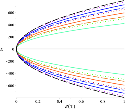
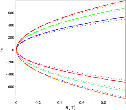
Figure 1: Plot of the energy versus the magnetic field, for $\lambda=0.4$; In Fig. (a), any value of the angular momentum quantum number $m$ being possible. The zero energy is present. In Fig. (b), we have the case for the allowed values of $m$ for which only the part of the energy spectrum containing the parameter $\lambda$ is present. The zero energy is absent.

In the last section, we have found the energy levels using the polar coordinates but we consider that the sample is not a disc, that is, it has a rectangular shape. This way, we start by considering the expression for the Hall conductivity obtained in Ref. [38] in the clean limit, that is,

$$\sigma_{xy}^{(1)} =-\frac{e^{2}N_{f}\mathrm{sign}(eB)}{4\pi}$$

$$\times\sum_{n=0}^{\infty}\alpha_{n}\left[\tanh\left(\frac{\mu+E_{n}}{T}\right)+\tanh\left(\frac{\mu-E_{n}}{T}\right)\right],$$ (32)

where $\alpha_{0}=1$ (for $n=0$) and $\alpha_{n}/\alpha_{0}=2$ (for $n\geq 1$).

This is related to the above-mentioned smaller degeneracy of the $n=0$ Landau level. In our case, we have observed that such AB elastic field, with non integer $\lambda$, fails to observe the zero Landau level around one valley. Then, the degeneracy of energy levels related to these valleys is broken due to the pseudo AB field in this situation. Moreover, the energy levels are shifted differently around the each valley. The consequence is that we have to consider a sum in the valley index. Therefore, we have the Hall conductivity as,

$$\sigma_{xy} =\sigma_{xy}^{(1)}-\frac{e^{2}N_{f}\mathrm{sign}(eB)}{4\pi}\sum_{k=K}^{K^{\prime}}\sum_{n^{\prime}=0}^{\infty}\alpha_{n^{\prime}}\left(\lambda\right)$$

$$\times\left[\tanh\left(\frac{\mu+E^{k}_{n^{\prime}}\left(\lambda\right)}{T}\right)+\tanh\left(\frac{\mu-E^{k}_{n^{\prime}}\left(\lambda\right)}{T}\right)\right],$$ (33)

where $\alpha_{n^{\prime}}\left(\lambda\right)=1,$ for any $n^{\prime}$.

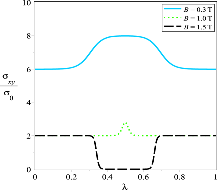
Figure 2: Plot of Hall conductivity versus the elastic parameter $\lambda$ for $T=3\mathrm{K}$ (we ignore the terms which do not contain $\lambda$). Notice that it is symmetric around $\lambda=0.5$

In Fig. 2, we plot the Hall conductivity versus the elastic parameter $\lambda$, which shows that the Hall conductivity is symmetric around $\lambda=0.5$. In Fig. 3(a), we plot the Hall conductivity versus the magnetic field for different values of $\lambda$. In the Quantum Hall effect in graphene ($\lambda\equiv 0$), the quantum Hall conductivity exhibits the standard plateaux at all integer $n$ of $4e^{2}/h$, for $n=1,2,3..$, and $2e^{2}/h$ for $n=0$. For $\lambda\neq 0$, the plateaux are shifted to higher magnetic fields. The presence of the Pseudo AB field introduce intermediate plateaux between them. These extra plateaux are not observed for $\lambda=0.5$, since the valley degeneracy is recovered in this case. In Fig. 4(a) it is depicted the Hall conductivity versus the chemical potential for some values of $\lambda$. We observe the same fact, that is, the quantum Hall conductivity exhibits the standard plateaux at all integer $n$ of $2e^{2}/h$. In the Fig. 3(b) and 4(b), we analyze the case supposing that the system is prepared so that only the energies containing the parameter $\lambda$ are possible to be occupied by the electrons. This happens if only either the condition $m-\lambda>1$ (regular solutions) or $-1<m-\lambda<0$ (irregular solutions) hold. In this case, a Hall plateau develops at $\sigma_{xy}=0$ (filling factor $\nu=0$), in contrast to what we have discussed above. This happens when a gap is opened in the energy bands of graphene.

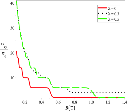
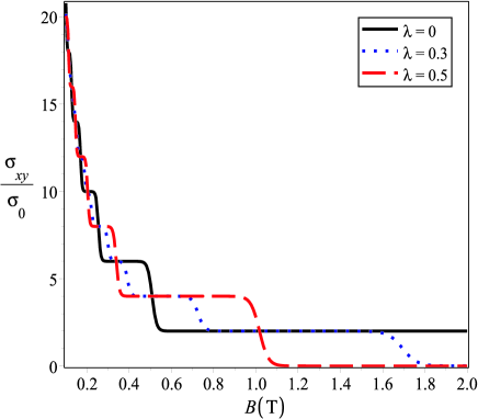
Figure 3: Plot of the Hall conductivity versus the magnetic field for $T=3K$: $\lambda=0$ (absence of the elastic interaction), $\lambda=0.3$ and $\lambda=0.5$; In Fig. (a), any value of the angular momentum quantum number $m$ being possible (see Fig. 1(a)). The plateaux shift to higher magnetic fields. In Fig. (b), we have the case for the allowed values of $m$ for which only the part of the energy spectrum containing the parameter $\lambda$ is present (see Fig. 1(b)).

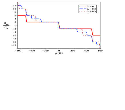
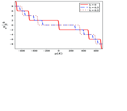
Figure 4: Plot of the Hall conductivity versus the chemical potential $\mu$ for $T=3K$, $\lambda=0$ (absence of the elastic interaction), $\lambda=0.3$ and $\lambda=0.5$; In Fig. (a), any value of the angular momentum quantum number $m$ being possible (see Fig. 1(a) and Fig. 3(a)). In Fig. (b), we have the case for the allowed values of $m$ for which only the part of the energy spectrum containing the parameter $\lambda$ is present (see Fig. 1(b) and Fig. 3(b)). In this case, a plateau develops at a null filling factor.

5 Concluding Remarks

In this work, we investigated how the relativistic Landau levels and the quantum Hall conductivity are modified if fermions on graphene are held in the presence of a constant orthogonal magnetic field together with a AB pseudo-field. We considered it mathematically modeled as in the case of a thin solenoid in the case of an actual AB field. We were able to study this problem analytically since our squared Dirac equation yielded a differential equation whose solutions are well established in terms of Hypergeometric series, which appear in many contexts, helping addressing different physical problems analytically as we did here. We have observed that, for certain constraints on the orbital angular momentum eigenvalues allowed for the system ($m-\lambda\geq 1$ for regular wavefunctions and $-1<m-\lambda\leq 0$ for irregular ones), it fails to observe the zero Landau level around both valleys, $K$ and $K^{\prime}$. The consequence is that a Hall plateau develops at the filling factor $\nu=0$. Then, the quantum Hall conductivity showed the standard plateaux at all integer $n$ of $2e^{2}/h$ except for $n=0$. This is in contrast to the usual Quantum Hall effect in graphene, where the quantum Hall conductivity exhibits the standard plateaux at all integer $n$ of $4e^{2}/h$, for $n=1,2,3..$, and $2e^{2}/h$ for $n=0$. Without such constraints in the orbital angular momentum eigenvalues, the the zero Landau level around both valleys are recovered and we have the plateaux at all integer $n$ of $2e^{2}/h$ including that for $n=0$.

As a final word, we theoretically described a way to manipulate the relativistic Landau levels by assuming the existence of an AB pseudo field. Graphene under different position-dependent magnetic fields was investigated theoretically in reference [19, 20, 21, 22, 23]. It would also be interesting to investigate them as pseudo magnetic fields combined with a constant magnetic field as we have done in this work. If either simulations or experiments involving graphene fail to observe the zero Landau level, the presence of varying pseudo magnetic fields should be investigated. The problem addressed here is closed related to but not equal to the case where topological defects on a graphene sheet are present, since their existence also split the zero energy [39, 40]. Here, we have showed how a delta like interaction can affect the quantum hall system and it is important to have those questions in mind if one is interested to probe the effects of a singular curvature in these systems.

References

- Landau and Lifschitz [1981] L. D. Landau, E. M. Lifschitz, Quantum Mechanics, Pergamon, Oxford, 1981.
- Aharonov and Bohm [1959] Y. Aharonov, D. Bohm, Phys. Rev. 115 (1959) 485.
- Tan and Inkson [1996] W.-C. Tan, J. C. Inkson, Semicond. Sci. Technol. 11 (1996) 1635–.
- Ikhdair et al. [2015] S. M. Ikhdair, B. J. Falaye, M. Hamzavi, Ann. Phys. 353 (2015) 282 – 298.
- Hamzavi et al. [2014] M. Hamzavi, S. M. Ikhdair, B. J. Falaye, Ann. Phys. 341 (2014) 153 – 163.
- Trevisan et al. [2014] L. A. Trevisan, C. Mirez, F. M. Andrade, Few-Body Syst. 55 (2014) 1055.
- Geim and Novoselov [2007] A. K. Geim, K. S. Novoselov, Nat. Mater. 6 (2007) 183–191.
- Castro Neto et al. [2009] A. H. Castro Neto, F. Guinea, N. M. R. Peres, K. S. Novoselov, A. K. Geim, Rev. Mod. Phys. 81 (2009) 109.
- Balandin et al. [2008] A. A. Balandin, S. Ghosh, W. Bao, I. Calizo, D. Teweldebrhan, F. Miao, C. N. Lau, Nano Lett. 8 (2008) 902.
- Schwierz [2010] F. Schwierz, Nat Nano 5 (2010) 487–496.
- Li et al. [2012] J. Li, X. Cheng, A. Shashurin, M. Keidar, Graphene Vol.01No.01 (2012) 13.
- Sols et al. [2007] F. Sols, F. Guinea, A. H. C. Neto, Phys. Rev. Lett. 99 (2007) 166803.
- Han et al. [2007] M. Y. Han, B. Özyilmaz, Y. Zhang, P. Kim, Phys. Rev. Lett. 98 (2007) 206805.
- Mucciolo et al. [2009] E. R. Mucciolo, A. H. Castro Neto, C. H. Lewenkopf, Phys. Rev. B 79 (2009) 075407.
- Vozmediano et al. [2010] M. Vozmediano, M. Katsnelson, F. Guinea, Physics Reports 496 (2010) 109–148.
- Guinea et al. [2010] F. Guinea, M. I. Katsnelson, A. K. Geim, Nat Phys 6 (2010) 30–33.
- Verbiest et al. [2015] G. J. Verbiest, S. Brinker, C. Stampfer, Phys. Rev. B 92 (2015) 075417.
- Verbiest et al. [2016] G. J. Verbiest, C. Stampfer, S. E. Huber, M. Andersen, K. Reuter, Phys. Rev. B 93 (2016) 195438.
- Setare and Olfati [2007] M. R. Setare, G. Olfati, Physica Scripta 75 (2007) 250–.
- Kuru et al. [2009] . Kuru, J. Negro, L. M. Nieto, Journal of Physics: Condensed Matter 21 (2009) 455305–.
- Hartmann and Portnoi [2014] R. R. Hartmann, M. E. Portnoi, Phys. Rev. A 89 (2014) 012101.
- Eshghi and Mehraban [2016a] M. Eshghi, H. Mehraban, Journal of Mathematical Physics 57 (2016a).
- Eshghi and Mehraban [2016b] M. Eshghi, H. Mehraban, Comptes Rendus Physique (2016b).
- de Juan et al. [2011] F. de Juan, A. Cortijo, M. A. H. Vozmediano, A. Cano, Nat Phys 7 (2011) 810–815.
- Filgueiras et al. [2010] C. Filgueiras, E. O. Silva, W. Oliveira, F. Moraes, Ann. Phys. (NY) 325 (2010) 2529.
- Filgueiras et al. [2012] C. Filgueiras, E. O. Silva, F. M. Andrade, J. Math. Phys. 53 (2012) 122106.
- Andrade and Silva [2013] F. M. Andrade, E. O. Silva, Phys. Lett. B 719 (2013) 467–471.
- Andrade et al. [2013] F. M. Andrade, E. O. Silva, M. Pereira, Ann. Phys. (NY) 339 (2013) 510–530.
- Andrade et al. [2012] F. M. Andrade, E. O. Silva, M. Pereira, Phys. Rev. D 85 (2012) 041701(R).
- Khalilov [2010] V. Khalilov, Theor. Math. Phys. 163 (2010) 511–516.
- Alford et al. [1989] M. Alford, J. March-Russell, F. Wilczek, Nucl. Phys. B 328 (1989) 140–158.
- Albeverio et al. [2004] S. Albeverio, F. Gesztesy, R. Hoegh-Krohn, H. Holden, Solvable Models in Quantum Mechanics, AMS Chelsea Publishing, Providence, RI, second edition, 2004.
- Bulla and Gesztesy [1985] W. Bulla, F. Gesztesy, J. Math. Phys. 26 (1985) 2520.
- Reed and Simon [1975] M. Reed, B. Simon, Methods of Modern Mathematical Physics. II. Fourier Analysis, Self-Adjointness., Academic Press, New York - London, 1975.
- Abramowitz and Stegun [1972] M. Abramowitz, I. A. Stegun (Eds.), Handbook of Mathematical Functions, New York: Dover Publications, 1972.
- Khalilov and Mamsurov [2009] V. Khalilov, I. Mamsurov, Theor. Math. Phys. 161 (2009) 1503–1512.
- Khalilov [2014] V. Khalilov, Eur. Phys. J. C 74 (2014) 1–7–.
- Gusynin and Sharapov [2006] V. P. Gusynin, S. G. Sharapov, Phys. Rev. B 73 (2006) 245411.
- Bueno et al. [2012] M. J. Bueno, C. Furtado, A. M. de M. Carvalho, The European Physical Journal B 85 (2012) 53–.
- Biswas and Son [2016] R. R. Biswas, D. T. Son, Proceedings of the National Academy of Sciences 113 (2016) 8636–8641.