Abstract

This paper studies systematic exploration for reinforcement learning with rich observations and function approximation. We introduce a new model called contextual decision processes, that unifies and generalizes most prior settings. Our first contribution is a complexity measure, the Bellman rank, that we show enables tractable learning of near-optimal behavior in these processes and is naturally small for many well-studied reinforcement learning settings. Our second contribution is a new reinforcement learning algorithm that engages in systematic exploration to learn contextual decision processes with low Bellman rank. Our algorithm provably learns near-optimal behavior with a number of samples that is polynomial in all relevant parameters but independent of the number of unique observations. The approach uses Bellman error minimization with optimistic exploration and provides new insights into efficient exploration for reinforcement learning with function approximation.

1 Introduction

How can we tractably solve sequential decision making problems where the agent receives rich observations?

In this paper, we study this question by considering reinforcement learning (RL) problems where the agent receives rich sensory observations from the environment, forms complex contexts from the sensorimotor streams, uses function approximation to generalize to unseen contexts, and must engage in systematic exploration to efficiently learn to complete tasks. Such problems are at the core of empirical reinforcement learning research (e.g., (Mnih et al., 2015; Bellemare et al., 2016)), yet no existing theory provides rigorous and satisfactory guarantees in a general setting.

To answer the question, we propose a new formulation, which we call Contextual Decision Processes (CDPs), to capture a large class of sequential decision-making problems: CDPs generalize MDPs where the state forms the context (Example 1), and POMDPs where the history forms the context (Example 2). We describe CDPs formally in Section 2, and the learning goal is to find a near-optimal policy for a CDP in a sample-efficient manner.

A structural assumption.

When the context space is very large or infinite, as is common in practice, lower bounds that are exponential in the problem horizon preclude efficient learning of CDPs, even when simple function approximators are used. However, RL problems arising in applications are often far more benign than the pathological lower bound instances, and we identify a structural assumption capturing this intuition. As our first major contribution, we define a notion of Bellman factorization (Definition 5) in Section 3, and focus on problems with low Bellman rank.

Model	tabular MDP	low-rank MDP	reactive POMDP	reactive PSR	LQR
Bellman rank	# states	rank	# hidden states	PSR rank	# state variables
PAC Learning	known	new	extended	new	known

Table 1: Summary of settings that admit low Bellman rank, with formal statements in Section 3 (Proposition 1 to 5, from left to right in the table). The 2nd row gives the parameters that bound the Bellman rank. In the 3rd row, “known” means that sample-efficient algorithms already exist for this setting (e.g., tabular MDPs), “extended” means results here substantially extend previous work (e.g., POMDPs with large observation spaces and reactive value functions (Krishnamurthy et al., 2016)) and “new” means our result gives the first sample-efficient algorithm (e.g., MDPs with low-rank transition dynamics).

At a high level, Bellman rank is a form of algebraic dimension on the interplay between the CDP and the value-function approximator that we show is small for many natural settings. For example, every MDP with a tabular value-function has Bellman rank bounded by the rank of its transition matrix, which is at most the number of states but can be considerably smaller. For a POMDP with reactive value-functions, the Bellman rank is at most the number of hidden states and has no dependence on the observation space. We provide other instances of low Bellman rank including Linear Quadratic Regulators and Predictive State Representations. Overall, CDPs with a small Bellman rank yield a unified framework for a large class of sequential decision making problems.

A new algorithm.

Our second contribution is a new algorithm for episodic reinforcement learning called Olive (Optimism Led Iterative Value-function Elimination), detailed in Section 4.1. Olive combines optimism-driven exploration and Bellman error-based search in a new way crucial for theoretical guarantees.

The algorithm is an iterative procedure that successively refines a space of candidate Q-value functions $\mathcal{F}$. At iteration $t$, it first finds the surviving value function $f\in\mathcal{F}_{t}$ that predicts the highest value on the initial context distribution. By collecting a few trajectories according to $f$’s greedy policy, $\pi_{f}$, we can verify this prediction. If the attained value is close to the prediction, our algorithm terminates and outputs $f$. If not, we eliminate all surviving $f^{\prime}\in\mathcal{F}_{t}$ which violate certain Bellman equations on trajectories sampled using $\pi_{f}$. $\mathcal{F}_{t+1}$ is set to all the surviving functions and this process repeats.

A PAC guarantee.

We prove that Olive performs sample-efficient learning in CDPs with a small Bellman rank (See Section 4.2). Concretely, when the optimal value-function in a CDP can be represented by the function approximator $\mathcal{F}$, the algorithm uses $\tilde{\mathcal{O}}(M^{2}H^{3}K\log(N/\delta)/\epsilon^{2})$ trajectories to find an $\epsilon$-suboptimal policy, where $M$ is the Bellman rank, $H$ is the horizon (the length of an episode), $K$ is the number of actions, $N$ is the cardinality of $\mathcal{F}$, and $\delta$ is the failure probability.

Importantly, the sample complexity bound has a logarithmic dependence on $\mathcal{F}$, thus enabling powerful function approximation, and no direct dependence on the size of the context space, which can be very large or even infinite. As many existing models, including the ones mentioned above, have low Bellman rank, the result immediately implies sample-efficient learning in all of these settings, as highlighted in Table 1.

We also present several extensions of the main result, showing robustness to the failure of the assumption that the optimal value-function is captured by the function approximator, adaptivity to unknown Bellman rank, and extension to infinite function classes of bounded statistical complexity. Altogether, these results show that the notion of Bellman rank robustly captures the difficulty of exploration in sequential decision-making problems.

To summarize, this work advances our understanding in reinforcement learning with complex observations where long-term planning and exploration are critical. There are, of course, several additional questions that must be resolved before we have satisfactory tools for these problems. The biggest drawback of Olive is its computational complexity, which is polynomial in the number of value functions and hence intractable for the powerful classes of interest. This issue must be addressed before we can empirically evaluate the effectiveness of the proposed algorithm. We leave this and other open questions for future work.

Related work.

There is a rich body of theoretical literature on learning Markov Decision Processes (MDPs) with small state spaces (Kearns and Singh, 2002; Brafman and Tennenholtz, 2003; Strehl et al., 2006), with an emphasis on sophisticated exploration techniques that find near-optimal policies in a sample-efficient manner. While there have been attempts to extend these techniques to large state spaces (Kakade et al., 2003; Jong and Stone, 2007; Pazis and Parr, 2016), these approaches fail to be a good fit for practical scenarios where the environment is typically perceived through complex sensory observations such as image, text, or audio signals. Alternatively, Monte Carlo Tree Search (MCTS) methods can handle arbitrarily large state spaces, but only at the cost of exponential dependence on the planning horizon (Kearns et al., 2002; Kocsis and Szepesvári, 2006). Our work departs from these existing efforts by aiming for a sample complexity that is independent of the size of the context space and at most polynomial in the horizon. Similar goals have been attempted by Wen and Van Roy (2013) and Krishnamurthy et al. (2016) where attention is restricted to decision processes with deterministic dynamics and special structures. In contrast, we study a much broader class of problems with relatively mild conditions.

On the empirical side, the prominent recent success on both the Atari platform (Mnih et al., 2015; Wang et al., 2015) and Go (Silver et al., 2016) have sparked a flurry of research interest. These approaches leverage advances in deep learning for powerful function approximation, while, in most cases, using simple heuristic strategies, such as $\epsilon$-greedy, for exploration. More advanced exploration strategies include extending the methods for small state spaces (e.g., the use of pseudo-counts in Bellemare et al. (2016)), and combining MCTS with function approximation (e.g., Silver et al. (2016)). Unfortunately, both types of approaches often require strong domain knowledge and large amounts of data to be successful.

Hallak et al. (2015) have proposed a setting called Contextual MDPs, where a context refers to some static information that can be used to generalize across many similar MDPs. In this paper, a context is most similar to state features in the RL literature and is a natural generalization of the notion of context as in the contextual bandit literature (Langford and Zhang, 2008).

2 Contextual Decision Processes (CDPs)

We introduce a new model, called a Contextual Decision Process, as a unified framework for reinforcement learning with rich observations. We first present the model, before the relevant notation and definitions.

2.1 Model and Examples

Contextual Decision Processes make minimal assumptions to capture a very general class of RL problems and are defined as follows.

Definition 1 (Contextual Decision Process (CDP)).

A (finite-horizon) Contextual Decision Process (CDP for short) is defined as a tuple $(\mathcal{X},\mathcal{A},H,P)$, where $\mathcal{X}$ is the context space, $\mathcal{A}$ is the action space, and $H$ is the horizon of the problem. $P=(P_{\varnothing},P_{+})$ is the system descriptor, where $P_{\varnothing}\in\Delta(\mathcal{X})$ is a distribution over initial contexts, that is $x_{1}\sim P_{\varnothing}$, and $P_{+}:(\mathcal{X}\times\mathcal{A}\times\mathbb{R})^{*}\times\mathcal{X}\times\mathcal{A}\to\Delta(\mathbb{R}\times\mathcal{X})$ elicits the next reward and context from the interactions so far $x_{1},a_{1},r_{1},\ldots,x_{h},a_{h}$:

$$(r_{h},x_{h+1})\sim P_{+}(x_{1},a_{1},r_{1},\ldots,x_{h},a_{h}).$$

In a CDP, the agent’s interaction with the environment proceeds in episodes. In each episode, the agent observes a context $x_{1}$, takes action $a_{1}$, receives reward $r_{1}$ and observes $x_{2}$, repeating $H$ times. A policy $\pi:\mathcal{X}\to\mathcal{A}$ specifies the decision-making strategy of an agent, that is $a_{h}=\pi(x_{h}),~{}\forall h\in[H]$, and induces a distribution over the trajectory $(x_{1},a_{1},r_{1},\ldots,x_{H},a_{H},r_{H},x_{H+1})$ according to the system descriptor $P$. The value of a policy, $V^{\pi}$, is defined as

$$V^{\pi}=\mathbb{E}_{P}\left[\textstyle\sum_{h=1}^{H}r_{H}~{}\Big{|}~{}a_{1:H}\sim\pi\right],$$ (1)

where $a_{1:H}\sim\pi$ abbreviates for $a_{1}=\pi(x_{1}),\ldots,a_{H}=\pi(x_{H})$. Here, and in the sequel, the expectation is always taken over contexts and rewards drawn according to the system descriptor $P$, so we suppress the subscript $P$ for brevity. The goal of the agent is to find a policy $\pi$ that attains the largest value.

Below we show that CDPs capture classical RL models, including MDPs and POMDPs, and the optimal policies can be expressed as a function of appropriately chosen contexts.

Example 1 (MDPs with states as contexts).

Consider a finite-horizon MDP $({\mathcal{S}},\mathcal{A},H,\Gamma_{1},\Gamma,R)$, where ${\mathcal{S}}$ is the state space, $\mathcal{A}$ is the action space, $H$ is the horizon, $\Gamma_{1}\in\Delta({\mathcal{S}})$ is the initial state distribution, $\Gamma:{\mathcal{S}}\times\mathcal{A}\to\Delta({\mathcal{S}})$ is the state transition function, $R:{\mathcal{S}}\times\mathcal{A}\to\Delta([0,1])$ is the reward function, and an episode takes the form of $(s_{1},a_{1},r_{1},\ldots,s_{H},a_{H},r_{H})$. We can convert the MDP to a CDP $(\mathcal{X},\mathcal{A},H,P)$ by letting $\mathcal{X}={\mathcal{S}}\times[H]$ and $x_{h}=(s_{h},h)$, which allows the set of policies $\{\mathcal{X}\to\mathcal{A}\}$ to contain the optimal policy (Puterman, 1994). The system descriptor is $P=(P_{\varnothing},P_{+})$, where $P_{\varnothing}(x_{1})=\Gamma_{1}(s_{1})$, and $P_{+}(r_{h},x_{h+1}\,|\,x_{1},a_{1},r_{1},\ldots,x_{h},a_{h})=R(r_{h}|s_{h},a_{h})\,\Gamma(s_{h+1}|s_{h},a_{h})$.

The system descriptor for a particular model is usually obvious from the definitions, and here we give its explicit form as an illustration. We omit the specification of system descriptor in the remaining examples.

Next we turn to POMDPs. It might seem that a CDP describes a similar process as a POMDP but limits the agent’s decision-making strategies to memoryless (or reactive) policies, as we only consider policies in $\{\mathcal{X}\to\mathcal{A}\}$. This is not true. We clarify this issue by showing that we can use the history as context, and the induced CDP suffers no loss in the ability to represent optimal policies.

Example 2 (POMDPs with histories as contexts).

Consider a finite-horizon POMDP with a hidden state space ${\mathcal{S}}$, an observation space $\mathcal{O}$, and an emission process $D_{s}$ that associates each $s\in{\mathcal{S}}$ with a distribution over $\mathcal{O}$. We can convert the POMDP to a CDP $(\mathcal{X},\mathcal{A},H,P)$ by letting $\mathcal{X}=(\mathcal{O}\times\mathcal{A}\times\mathbb{R})^{*}\times\mathcal{O}$ and $x_{h}=(o_{1},a_{1},r_{1},\ldots,o_{h})$ is the observed history at time $h$.

It is also clear from this example that we can assume contexts are Markovian in CDPs without loss of generality, as we can always use history as context. While we do not commit to this assumption to allow for a flexible framework with simple notation (see Example 3), we later connect to well-known results in MDP literature based on this observation so that readers can transfer insights from MDPs to CDPs.

Example 3 (POMDPs with sliding windows of observations as contexts).

In some application scenarios, partial observability can be resolved by using a small sliding window: for example, in Atari games, it is common to keep track of the last $4$ frames of images (Mnih et al., 2015). In this case, we can represent the problem as a CDP by letting $x_{h}=(o_{h-3},o_{h-2},o_{h-1},o_{h})$.

We hope these examples convince the reader of the flexibility of keeping contexts separate from intrinsic quantities such as states or observations. Finally, we introduce a regularity assumption on the rewards.

Assumption 1 (Boundedness of rewards).

We assume that regardless of how actions are chosen, for any $h=1,\ldots,H$, $r_{h}\geq 0$ and $\sum_{h=1}^{H}r_{h}\leq 1$ almost surely.

2.2 Value-based RL and Function Approximation

Now that we have a model in place, we turn to some important solution concepts.

A CDP makes no assumption on the cardinality of the context space, which makes it critical to generalize across contexts, since the agent might not encounter the same context twice. Therefore, we consider value-based RL with function approximation. That is, the agent is given a set of functions $\mathcal{F}\subseteq\mathcal{X}\times\mathcal{A}\to[0,1]$ and uses it to approximate an action-value function (or Q-value function). Without loss of generality we assume that $f(x_{H+1},a)\equiv 0$. For the purpose of presentation, we assume that $\mathcal{F}$ is a finite space with $|\mathcal{F}|=N<\infty$ for most of the paper. In Section 5.3 we relax this assumption and allow infinite function classes with bounded complexity.

As in typical value-based RL, the goal is to identify $f\in\mathcal{F}$ which respects a particular set of Bellman equations and achieves a high value with its greedy policy $\pi_{f}(x)=\mathop{\mathrm{argmax}}_{a\in\mathcal{A}}f(x,a)$. We next set up the appropriate extensions of Bellman equations to CDPs and the optimal value $V_{\mathcal{F}}^{\star}$ through a series of definitions. Unlike typical definitions in MDPs, these involve both the CDP and function approximator $\mathcal{F}$.

Definition 2 (Average Bellman error).

Given any policy $\pi:\mathcal{X}\to\mathcal{A}$ and a function $f:\mathcal{X}\times\mathcal{A}\to[0,1]$, the average Bellman error of $f$ under roll-in policy $\pi$ at level $h$ is defined as

$$\mathcal{E}(f,\pi,h)=\mathbb{E}\,\big{[}f(x_{h},a_{h})-r_{h}-f(x_{h+1},a_{h+1})~{}\big{|}~{}a_{1:h-1}\sim\pi,~{}a_{h:h+1}\sim\pi_{f}\big{]}.$$ (2)

In words, the average Bellman error measures the self-consistency of a function $f$ between its predictions at levels $h$ and $h+1$ when all the previous actions are taken according to some policy $\pi$. Given this definition, we now define a set of Bellman equations.

Definition 3 (Bellman equations and validity of $f$).

Given an $(f,\pi,h)$ triple, a Bellman equation posits $\mathcal{E}(f,\pi,h)=0$. We say $f\in\mathcal{F}$ is valid if the Bellman equation on $(f,\pi_{f^{\prime}},h)$ holds for every $f^{\prime}\in\mathcal{F},h\in[H]$.

Note that the validity assumption only considers roll-ins according to the greedy policies $\pi_{f}$, which is the natural policy class in a function approximation setting. In Section 5.2, we show how to incorporate a separate policy class in these definitions. In the MDP setting, each Bellman equation can be viewed as the linear combination of the standard Bellman optimality equations for $Q^{\star}$, where the coefficients are the probabilities with which the roll-in policy $\pi$ visits each state. This leads to the following consequence.

Fact 1 ($Q^{\star}$ is always valid).

Given an MDP and a space of functions $\mathcal{F}:{\mathcal{S}}\times[H]\times\mathcal{A}\to[0,1]$, if the optimal Q-value function of the MDP $Q^{\star}$ lies in $\mathcal{F}$, then in the corresponding CDP with $\mathcal{X}={\mathcal{S}}\times[H]$, $Q^{\star}$ is valid.

While $Q^{\star}$ satisfies the Bellman equations and yields the optimal policy $\pi^{\star}=\pi_{Q^{\star}}$, there can be other functions which also satisfy the equations while yielding suboptimal policies. This happens because Eq. (2) only considers $a_{h}$ drawn according to $\pi_{f}$ and does not use the values on other actions. For instance, consider a CDP where at every context, action $a$ always gets a reward of 0 and action $a^{\prime}$ always gets a reward of 1. A function that predicts $f(x,a)=f(x,a^{\prime})=0~{}\forall x,a$ is trivially valid as long as tie-breaks always favor $a$.

Since validity alone does not imply that we get a good policy, it is natural to search for a valid value function which also induces a high-value policy. We formalize this goal in the next definition.

Definition 4 (Optimal value).

Define $f^{\star}=\mathop{\mathrm{argmax}}_{f\in\mathcal{F}:\,f\textrm{\,is valid}}V^{\pi_{f}},$ and $V_{\mathcal{F}}^{\star}=V^{\pi_{f^{\star}}}.$

Fact 2.

For the same setting as in Fact 1, when $Q^{\star}\in\mathcal{F}$, we have $f^{\star}=Q^{\star}$, and $V_{\mathcal{F}}^{\star}=V^{\star}$, which is the optimal long-term value.

Definition 4 implicitly assumes that there is at least one valid $f\in\mathcal{F}$. This is weaker than the realizability assumption made in the value-based RL literature, that $\mathcal{F}$ contains the optimal Q-value function of an MDP $Q^{\star}$ (Antos et al., 2008; Krishnamurthy et al., 2016). Indeed, the setup subsumes realizability, as evidenced by Fact 1 and 2. When $Q^{\star}\in\mathcal{F}$, the algorithm aims to identify a policy achieving value close to $V^{\star}$, the optimal value achievable by any agent. When no functions in $\mathcal{F}$ approximate $Q^{\star}$ well, finding the best valid value function is still a meaningful and non-trivial objective. In this sense, our work makes substantially weaker realizability-type assumptions than prior theoretical results for value-based RL (Antos et al., 2008; Krishnamurthy et al., 2016), which assume $Q^{\star}\in\mathcal{F}$ often in addition to several stronger requirements.

Approximation to Bellman Equations.

In general, $\mathcal{F}$ may not contain $Q^{*}$, or any valid functions at all, which makes our learning goal trivial. It is desirable to have an algorithm robust to such a scenario, and we show how our algorithm requires only an approximate notion of validity in Section 5.4, implying a graceful degradation in the results.

3 Bellman Factorization and Bellman Rank

CDPs are general models for sequential decision making, but are there efficient RL algorithms for them?

Unfortunately, without further assumptions, learning in CDPs is generally hard, since they subsume MDPs and POMDPs with arbitrarily large state/observation spaces. Moreover, a function class $\mathcal{F}$ with low statistical complexity, which would generalize effectively in a standard supervised learning setting with a fixed data distribution, does not overcome this difficulty in CDPs where the data distribution crucially depends on the agent’s policy. In particular, even when $\log N$, the statistical complexity for finite classes, is small, there exists an $\Omega(K^{H})$ lower bound on the sample complexity of learning CDPs. The result is due to Krishnamurthy et al. (2016), and is included in Appendix A.1 for completeness.

While exponential lower bounds for learning CDPs exist, they are fairly pathological, and most real problems have substantially more structure. To capture these realistic instances and circumnavigate the lower bounds, we propose a new complexity measure and restrict our attention to settings where this measure is low. As we will see, this measure is naturally small for many existing models, and, when it is small, efficient reinforcement learning is possible.

The complexity measure we propose is a structural characterization of the set of Bellman equations induced by the CDP and the value-function class (recall Definition 2) that we need to check to find valid functions. While checking validity by enumeration is intractable for large $\mathcal{F}$, observe that the Bellman equations are structured in tabular MDPs: the average Bellman error under any roll-in policy is a stochastic combination of the single-state errors, and checking the single-state errors (which is tractable) is sufficient to guarantee validity. This observation hints toward a more general phenomenon: whenever the collection of Bellman errors across all roll-in policies can be concisely represented, we may be able to check the validity of all functions in a tractable way.

This intuition motivates a new complexity measure that we call the Bellman rank. Define the Bellman error matrices, one for each $h$, to be $|\mathcal{F}|\times|\mathcal{F}|$ matrices where the $(f,f^{\prime})^{\textrm{th}}$ entry is the Bellman error $\mathcal{E}(f,\pi_{f^{\prime}},h)$. Informally, the Bellman rank for a CDP and a given value-function class $\mathcal{F}$ is a uniform upper bound on the rank of these $H$ Bellman error matrices.

Now we give the formal definition below.

Definition 5 (Bellman factorization and Bellman rank).

We say that a CDP $(\mathcal{X},\mathcal{A},H,P)$ and $\mathcal{F}\subset\mathcal{X}\times\mathcal{A}\to[0,1]$ admit Bellman factorization with Bellman rank $M$ and norm parameter $\zeta$, if there exists $\nu_{h}:\mathcal{F}\to\mathbb{R}^{M},\xi_{h}:\mathcal{F}\to\mathbb{R}^{M}$ for each $h\in[H]$, such that for any $f,f^{\prime}\in\mathcal{F},h\in[H]$,

$$\mathcal{E}(f,\pi_{f^{\prime}},h)=\langle\nu_{h}(f^{\prime}),\xi_{h}(f)\rangle,$$ (3)

and $\|\nu_{h}(f^{\prime})\|_{2}\cdot\|\xi_{h}(f)\|_{2}\leq\zeta<\infty$.

The exact factorization in Eq. (3) can be relaxed to an approximate version as is discussed in Section 5.4. In the remaining sections of this paper we introduce the main algorithm, and analyze its sample-efficiency in problems with low Bellman rank. In the remainder of this section we showcase the generality of Definition 5 by describing a number of common RL settings that have a small Bellman rank. Throughout, we see how the Bellman rank captures the process-specific structures that allow for efficient exploration. Proofs of all claims in this section are deferred to Appendix B.

We start with the tabular MDP setting, and show that the Bellman rank is at most the number of states.

Proposition 1 (Bellman rank bounded by number of states in MDPs).

Consider the MDP setting of Example 1 with the corresponding CDP. With any $\mathcal{F}\subset\mathcal{X}\times\mathcal{A}\to[0,1]$, this model admits a Bellman factorization with $M=|{\mathcal{S}}|$ and $\zeta=2\sqrt{M}$.

A related model introduced by Li (2009) for extending tabular PAC-MDP methods to large MDPs using a form of state abstractions also has low Bellman rank (See Appendix B.2).

The MDP example is particularly simple as each coordinate of the $M$-dimensional space corresponds to a state, which is observable. Our next few examples show that this is not necessary, and that Bellman factorization can be based on latent properties of the process. We next consider large MDPs whose transition dynamics have a low-rank structure. A closely related setting has been considered by Barreto et al. (2011, 2014) where the low-rank structure is exploited to speed up MDP planning, but prior to this work, no sample-efficient RL algorithms are known for this setting.

Proposition 2 (Bellman rank in low-rank MDPs, informally).

Consider the MDP setting of Example 1 with a transition matrix $\Gamma$ having rank at most $M$. The induced CDP along with any $\mathcal{F}\subset\mathcal{X}\times\mathcal{A}\to[0,1]$ admits a Bellman factorization with Bellman rank $M$.

The next example considers POMDPs with large observations spaces and reactive value functions, where the Bellman rank is at most the number of hidden states.

Proposition 3 (Bellman rank bounded by hidden states in reactive POMDPs).

Consider the POMDP setting of Example 3 with $|{\mathcal{S}}|<\infty$ and a sliding window of size 1 along with the induced CDP. Given any $\mathcal{F}\subset\mathcal{X}\times\mathcal{A}\to[0,1]$, this model admits a Bellman factorization with $M=|{\mathcal{S}}|$ and $\zeta=2\sqrt{M}$.

Proposition 2 and 3 can be proved under a unified model that generalizes POMDPs by allowing the transition function and the reward function to depend on the observation (See Figure 1 (a) – (c) for graphical representations of these models). This unified model captures the experimental settings considered in state-of-the-art empirical RL work (Figure 1 (d)), where agents act in a grid-world ($|{\mathcal{S}}|$ is small) and receives complex and rich observations such as raw pixel images ($|\mathcal{O}|$ is large). The model also subsumes and generalizes the setting of Krishnamurthy et al. (2016) which requires deterministic transitions in the underlying MDP. Our new algorithm eliminates the need for determinism, and still guarantee sample-efficient learning.

(a) MDP with low-rank transition dynamics. Gray nodes represent the hidden factors in the low-rank factorization.

(b) POMDP with reactive policy. Gray nodes represent hidden states.
 

(c) A unified model that subsumes (a) and (b) and yields low Bellman rank.

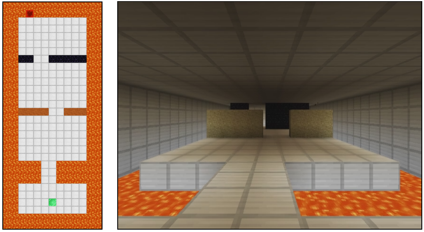
(d) A popular RL experiment setting (Johnson et al., 2016).

Figure 1: Example RL scenarios that yield low Bellman rank. No sample-efficient exploration strategies are known for these problems previously, so the algorithm and analysis provide the first PAC-Learning guarantees. (a) An MDP that has low-rank transition structure (see Proposition 2). The unlabelled nodes correspond to the hidden factors in the low-rank factorization, and can take $M$ different values. (b) A POMDP with reactive policies (see Proposition 3). The dashed arrow from $o$ to $a$ implies that we only consider policies that map $\mathcal{O}$ to $\mathcal{A}$ (the dependence on time step is made implicit). (c) A model that unifies (a) and (b), which still yields low Bellman rank (proof is in Appendix B). To embed (a) in (c), the observed states $s$ and $s^{\prime}$ in (a) become the observations $o$ and $o^{\prime}$ in (c). (d) A popular experiment setting in state-of-the-art empirical work. The environment is a grid-world (hence $|{\mathcal{S}}|$ is small and so is the Bellman rank), and the agent’s sensory inputs are raw pixel images (hence $|\mathcal{O}|$ is very large).

Next, we consider Predictive State Representations (PSRs), which are models of partially observable systems with parameters grounded in observable quantities (Littman et al., 2001). Similar to the case of POMDPs, we can bound the Bellman rank in terms of the rank of the PSR when the candidate value functions are reactive.

Proposition 4 (Bellman rank in PSRs, informally).

Consider a partially observable system with observation space $\mathcal{O}$, and the induced CDP $(\mathcal{X},\mathcal{A},H,P)$ with $x_{h}=(o_{h},h)$. If the linear dimension of the system (i.e., rank of its PSR model) is at most $L$, then given any $\mathcal{F}:\mathcal{X}\times\mathcal{A}\to[0,1]$, the Bellman rank is bounded by $LK$.

The last example considers a class of linear control problems well studied in control theory, called Linear Quadratic Regulators (LQRs). We show that the Bellman rank in LQRs is bounded by the dimension of the state space. Exploration in this class of problems has been previously considered by Osband and Van Roy (2014). Note that the algorithm to be introduced in the next section does not directly apply to LQRs due to the continuous action space, and adaptations that exploit the structure of the action space may be needed, which we leave for future work.

Proposition 5 (Bellman rank in LQRs, informally).

An LQR can be viewed as an MDP with continuous state space $\mathbb{R}^{d}$ and action space $\mathbb{R}^{K}$, where the dynamics are described by some linear equations. Given any function class $\mathcal{F}$ consisting of non-stationary quadratic functions of the state, the Bellman rank is bounded by $d^{2}+1$.

4 Algorithm and Main Results

In this section we present the algorithm for learning CDPs that have a Bellman factorization with a small Bellman rank and the main sample complexity guarantee. To aid presentation and help convey the main ideas, we make three simplifying assumptions:

1. We assume the Bellman rank parameter $M$ is known to the agent.

2. We assume the function class $\mathcal{F}$ is finite with $|\mathcal{F}|=N$.

3. We assume exact validity (Definition 3) and exact Bellman factorization (Definition 5).

All three assumptions can be relaxed, and we sketch these relaxations in Section 5.

We are interested in designing an algorithm for PAC Learning CDPs. We say that an algorithm PAC learns if given $\mathcal{F}$, two parameters $\epsilon,\delta\in(0,1)$, and access to a CDP, the algorithm outputs a policy $\hat{\pi}$ with $V^{\hat{\pi}}\geq V_{\mathcal{F}}^{\star}-\epsilon$ with probability at least $1-\delta$. The sample complexity is the number of episodes needed to achieve such a guarantee, and is typically expressed in terms of $\epsilon$, $\delta$ and other relevant parameters. The goal is to design an algorithm with sample complexity that is $\textrm{Poly}(M,K,H,1/\epsilon,\log(N),\log(1/\delta))$ where $M$ is the Bellman rank, $K$ is the number of actions, and $H$ is the time horizon. Importantly, the bound has no dependence on the number of unique contexts $|\mathcal{X}|$.

4.1 Algorithm

Pseudocode for the algorithm, which we call Olive (Optimism Led Iterative Value-function Elimination), is displayed in Algorithm 1. Theorem 1 describes how to set the parameters $n_{\textrm{est}},n_{\textrm{eval}},n$, and $\phi$.

At a high level, the algorithm aims to eliminate functions $f\in\mathcal{F}$ that fail to satisfy the validity condition in Definition 3. This is done by Lines 13 and 14 inside the loop of the algorithm. Observe that, since the actions $a_{h_{t}}$ are chosen uniformly at random, Eq. (5) produces an unbiased estimate of $\mathcal{E}(f,\pi_{t},h_{t})$, the average Bellman error for function $f$ on roll-in policy $\pi_{t}$ at time $h_{t}$. Thus, Eq. (6) eliminates functions that have high average Bellman error on this distribution, which means they fail to satisfy the validity criteria.

The other major component of the algorithm involves choosing the roll-in policy and level on which to do the learning step. At iteration $t$, we choose the roll-in policy $\pi_{t}$ optimistically, by choosing $f_{t}$ that predicts the highest value at the starting context distribution, and letting $\pi_{t}=\pi_{f_{t}}$. To pick the level, we compute $f_{t}$’s average Bellman error on its own roll-in distribution (Eq. (4)), and set $h_{t}$ to be any level for which this average Bellman error is high (See Line 11). As we will show, these choices ensure that substantial learning happens on each iteration, guaranteeing that the algorithm uses polynomially many episodes.

The last component is the termination criterion. The algorithm terminates if $f_{t}$ has small average Bellman error on its own roll-in distribution at all levels. This criteria guarantees that $\pi_{t}$ is near optimal.

Computationally, the algorithm requires enumeration of the value-function class, which we expect to be extremely large or infinite in practice. A computationally efficient implementation is essential for a practical algorithm, which is left to future work. We focus on the sample efficiency of the algorithm in this paper.

1:Collect $n_{\textrm{est}}$ trajectories with actions taken in an arbitrary manner; save initial contexts $\{x_{1}^{(i)}\}_{i=1}^{n_{\textrm{est}}}$.

2:Estimate the predicted value for each $f\in\mathcal{F}$: $\hat{V}_{f}=\frac{1}{n_{\textrm{est}}}\sum_{i=1}^{n_{\textrm{est}}}f(x_{1}^{(i)},\pi_{f}(x_{1}^{(i)}))$.

3:$\mathcal{F}_{0}\leftarrow\mathcal{F}$.

4:for $t=1,2,\ldots$ do

5:     Choose policy $f_{t}=\mathop{\mathrm{argmax}}_{f\in\mathcal{F}_{t-1}}\hat{V}_{f}$, $\pi_{t}=\pi_{f_{t}}$.

6:     Collect $n_{\textrm{eval}}$ trajectories $\{(x^{(i)}_{1},a^{(i)}_{1},r^{i}_{1},\ldots,x^{(i)}_{H},a^{(i)}_{H},r^{(i)}_{H})\}_{i=1}^{n_{\textrm{eval}}}$ by following $\pi_{t}$ (i.e. $a_{h}^{(i)}=\pi_{t}(x_{h}^{(i)})$ for all $h,i$).

7:     Estimate $\forall h\in[H]$,

$$\tilde{\mathcal{E}}(f_{t},\pi_{t},h)=\frac{1}{n_{\textrm{eval}}}\sum_{i=1}^{n_{\textrm{eval}}}\left[f_{t}(x^{(i)}_{h},a^{(i)}_{h})-r^{(i)}_{h}-f_{t}(x^{(i)}_{h+1},a^{(i)}_{h+1})\right].$$ (4)

8:     if $\sum_{h=1}^{H}\tilde{\mathcal{E}}(f_{t},\pi_{t},h)\leq 5\epsilon/8$ then

9:         Terminate and ouptut $\pi_{t}$.

10:     end if

11:     Pick any $h_{t}\in[H]$ for which $\tilde{\mathcal{E}}(f_{t},\pi_{t},h_{t})\geq 5\epsilon/8H$ (One is guaranteed to exist).

12:     Collect trajectories $\{(x_{1}^{(i)},a_{1}^{(i)},r_{1}^{(i)},\ldots,x_{H}^{(i)},a_{H}^{(i)},r_{H}^{(i)})\}_{i=1}^{n}$ where $a_{h}^{(i)}=\pi_{t}(x_{h}^{(i)})$ for all $h\neq h_{t}$ and $a_{h_{t}}^{(i)}$ is drawn uniformly at random.

13:     Estimate

$$\hat{\mathcal{E}}(f,\pi_{t},h_{t}) =\frac{1}{n}\sum_{i=1}^{n}\frac{\mathbf{1}[a_{h_{t}}^{(i)}=\pi_{f}(x_{h_{t}}^{(i)})]}{1/K}\Big{(}f(x_{h_{t}}^{(i)},a_{h_{t}}^{(i)})-r_{h_{t}}^{(i)}-f(x_{h_{t}+1}^{(i)},\pi_{f}(x_{h_{t}+1}^{(i)}))\Big{)}.$$ (5)

14:     Learn

$$\mathcal{F}_{t}=\left\{f\in\mathcal{F}_{t-1}:\left|\hat{\mathcal{E}}(f,\pi_{t},h_{t})\right|\leq\phi\right\}.$$ (6)

15:end for

Algorithm 1 Olive $(\mathcal{F},M,\zeta,\epsilon,\delta)$ – Optimism Led Iterative Value-function Elimination

Intuition for OLIVE. To convey intuition, it is helpful to ignore any sampling effects by replacing all empirical estimates with population values, and set $\epsilon$ to $0$. The first important fact is that the algorithm never eliminates a valid function, since the learning step in Eq. (6) only eliminates a function $f$ if we can find a distribution on which it has a large average Bellman error. If $f$ is valid, then $\mathcal{E}(f,\pi,h)=0$ for all $\pi,h$, so $f$ is never eliminated.

The second fact is that if a function $f$ is valid, then its predicted value is exactly the value achieved by the greedy policy $\pi_{f}$, that is $V_{f}=\mathbb{E}[f(x_{1},\pi_{f}(x_{1}))]=V^{\pi_{f}}$. This follows by telescoping the recursion in the definition of average Bellman error. Therefore, since $f_{t}$ is chosen optimistically as the maximizer of the value prediction among the surviving functions, and since we never eliminate valid functions, if Olive terminates, it must output a policy with value $V_{\mathcal{F}}^{\star}$. In the analysis, we incorporate sampling effects to derive robust versions of these facts so the algorithm always outputs a policy that is at most $\epsilon$-suboptimal.

The more challenging component is ensuring that the algorithm terminates in polynomially many iterations, which is critical for obtaining a polynomial sample complexity bound. This argument crucially relies on the Bellman factorization (recall Definition 5), which enables us to embed the distributions into $M$ dimensions and measure progress in this low-dimensional space.

For now, fix some $h$ and focus on the iterations when $h_{t}=h$. If we ignore sampling effects we can set $\phi=0$, and, by using the Bellman factorization to write $\mathcal{E}(f,\pi_{f_{t}},h)$ as an inner product, we can think of the learning step in Line 14 as introducing a homogeneous linear constraint on the set of $\xi_{h}(f)$ vectors, that is, $\langle\nu_{h}(f_{t}),\xi_{h}(f)\rangle=0$. Now, if we execute the learning step at level $h$ again in a later iteration $t^{\prime}$, we have $\langle\nu_{h}(f_{t^{\prime}}),\xi_{h}(f_{t^{\prime}})\rangle\neq 0$ from Line 11. Importantly, this means that $\nu_{h}(f_{t^{\prime}})$ must be linearly independent from previous $\nu_{h}(f_{t})$ since $\langle\nu_{h}(f_{t}),\xi_{h}(f_{t^{\prime}})\rangle=0$. In general, every time $h_{t}=h$, the number of linearly independent constraints increases by 1, and therefore the number of iterations where $h_{t}=h$ is at most the dimension of the space, which is $M$. Thus the Bellman rank leads to a bound on the number of iterations.

The above heuristic reasoning, despite relying on the brittle notion of linear independence, can be made robust. With sampling effects, rather than homogeneous linear equalities, the learning step for level $h$ introduces linear inequality constraints to the $\xi_{h}(f)$ vectors. But if $f^{\prime}$ is a surviving function that forces us to train at level $h$, it means that $\langle\nu_{h}(f^{\prime}),\xi_{h}(f^{\prime})\rangle$ is very large, while $\langle\nu_{h}(\cdot),\xi_{h}(f^{\prime})\rangle$ is very small for all previous $\nu_{h}(\cdot)$ vectors used in the learning step. Intuitively this means that the new $\nu(f^{\prime})$ vector is quite different from all of the previous ones. In our proof, we use a volumetric argument to show that this suffices to guarantee substantial learning takes place.

The optimistic choice for $f_{t}$ is critical for driving the agent’s exploration. With this choice, if $f_{t}$ is valid, then the algorithm terminates correctly, and if $f_{t}$ is not valid, then substantial progress is made. Thus the agent does not get stuck exploring with many valid but suboptimal functions, which could result in exponential sample complexity.

4.2 Sample Complexity

We now turn to the main result, which guarantees that Olive PAC-learns Contextual Decision Processes with polynomial sample complexity.

Theorem 1.

For any $\epsilon,\delta\in(0,1)$, any Contextual Decision Process and function class $\mathcal{F}$ that admits a Bellman factorization with parameters $M,\zeta$, run Olive with the following parameters:

$$\phi =\frac{\epsilon}{12H\sqrt{M}},\qquad n_{\textrm{est}}=\frac{32}{\epsilon^{2}}\log(6N/\delta),$$

$$n_{\textrm{eval}} =\frac{288H^{2}}{\epsilon^{2}}\log\left(\frac{12H^{2}M\log(6H\sqrt{M}\zeta/\epsilon)}{\delta}\right),$$

$$n =\frac{4608H^{2}MK}{\epsilon^{2}}\log\left(\frac{12NHM\log(6H\sqrt{M}\zeta/\epsilon)}{\delta}\right).$$

Then, with probability at least $1-\delta$, Olive halts and returns a policy $\hat{\pi}$ that satisfies $V^{\hat{\pi}}\geq V_{\mathcal{F}}^{\star}-\epsilon$ ($V_{\mathcal{F}}^{\star}$ in Definition 3), and the number of episodes required is at most

$$\tilde{\mathcal{O}}\left(\frac{M^{2}H^{3}K}{\epsilon^{2}}\log(N\zeta/\delta)\right).$$ (7)

According to this theorem, if a Contextual Decision Process and function class $\mathcal{F}$ admit a Bellman factorization with small Bellman rank and $\mathcal{F}$ contains valid functions, Olive is guaranteed to find a near optimal valid function using only polynomially many episodes. To our knowledge, our result is the most general polynomial sample complexity bound for reinforcement learning with rich observation spaces and function approximation, as many popular models are shown to admit small Bellman rank (see Section 3). The result also certifies that the notion of Bellman factorization, which is quite general, is sufficient for efficient exploration and learning in sequential decision making problems.

It is worth briefly comparing this result with prior work.

1. The most closely related result is the recent work of Krishnamurthy et al. (2016), who also consider episodic reinforcement learning with infinite observation spaces and function approximation. The model studied there is a form of Contextual Decision Process with Bellman rank $M$, so the result applies as is to that setting. Importantly, we eliminate the need for deterministic transitions, resolving one of their open problems. Moreover, the sample complexity bound improves the dependence on $H$ and $\epsilon$, at the cost of a worse dependence on $M$. We emphasize that this result applies to a much more general class of models.

2. Another related body of work provides sample complexity bounds for fitted value/policy iteration methods (e.g., (Munos, 2003; Antos et al., 2008; Munos and Szepesvári, 2008)). These works consider the infinite-horizon discounted MDP setting, and impose much stronger assumptions than we do including not only that the function class captures $Q^{\star}$, but also that it is approximately closed under Bellman update operators. More importantly, the analyses rely on the so-called concentrability coefficients to correct the mismatch between training and test distributions (Farahmand et al., 2010; Lazaric et al., 2012), implicitly assuming that an exploration distribution is given, hence these results do not address the exploration issue which is the main focus here.

3. Since CDPs include small-state MDPs (Kearns and Singh, 2002; Brafman and Tennenholtz, 2003; Strehl et al., 2006), the algorithm can be applied as is to these problems. Unfortunately, the sample complexity is polynomially worse than the state of the art $\tilde{\mathcal{O}}(\frac{M\textrm{poly}(H)K}{\epsilon^{2}}\log(1/\delta))$ bounds for PAC-learning MDPs (Dann and Brunskill, 2015). On the other hand, the algorithm also applies to MDPs with infinite state spaces with Bellman factorizations, which cannot be handled by tabular methods.

4. This approach applies to learning reactive policies in POMDPs (see Proposition 3). Azizzadenesheli et al. (2016) provides a sample-efficient algorithm in a closely related setting, where both the observation space and the hidden-state space are small in cardinality. While their approach does not require realizable value-functions, the sample complexity depends polynomially on the number of unique observations, and the method relies on additional mixing assumptions, which we do not require.

5. Finally, Contextual Decision Processes also encompass contextual bandits, where the optimal sample complexity is $O(K\log(N)/\epsilon^{2})$ (Agarwal et al., 2012). As contextual bandits have $M=1$ and $H=1$, Olive achieves optimal sample complexity in this special case.

Turning briefly to lower bounds, since the CDP setting with Bellman factorization is new, general lower bounds for the broad class do not exist. However, we can use MDP lower bounds for guidance on the question of optimality, since the small-state MDPs in Example 1 are a special case. While no existing MDP lower bounds apply as is (because formulations vary), in Appendix A.2 we adapt ideas from Auer et al. (2002) to obtain a $\Omega(MKH/\epsilon^{2})$ sample complexity lower bound for learning the MDPs in Example 1.

Comparing with this lower bound, the sample complexity in Theorem 1 is worse in $M,H$, and $\log(N)$ factors, but of course the small-state MDP is a significantly simpler special case. We leave as future work the question of optimal sample complexity for learning CDPs with low Bellman rank.

5 Extensions

We introduce four important extensions to the algorithm and analysis.

5.1 Unknown Bellman Rank

The first extension eliminates the need to know $M$ in advance (note that Algorithm 1 requires $M$ as an input parameter). A simple procedure described in Algorithm 2, can guess the value of $M$ on a doubling schedule and handle this situation with no consequences to asymptotic sample complexity.

Algorithm 2 GuessM$(\mathcal{F},\zeta,\epsilon,\delta)$

1:for $i=1,2,\ldots$ do

2:     $M^{\prime}\leftarrow 2^{i}$.

3:     Call $\textsc{Olive}(\mathcal{F},M^{\prime},\epsilon,\frac{\delta}{i(i+1)})$ with parameters specified on Theorem 1.

4:     Terminate the subroutine when $t>HM^{\prime}\log\left(\frac{6H\sqrt{M^{\prime}}\zeta}{\epsilon}\right)/\log(5/3)$ in Line 4 (the for-loop).

5:     if a policy $\pi$ is returned from Olive then return $\pi$.

6:     end if

7:end for

Theorem 2.

For any $\epsilon,\delta\in(0,1)$, any Contextual Decision Process and function class $\mathcal{F}$ that admits a Bellman factorization with parameters $M,\zeta$, if we run GuessM$(\mathcal{F},\epsilon,\delta)$, then with probability at least $1-\delta$, Olive halts and returns a policy which satisfies $V^{\hat{\pi}}\geq V_{\mathcal{F}}^{\star}-\epsilon$, and the number of episodes required is at most

$$\tilde{\mathcal{O}}\left(\frac{M^{2}H^{3}K}{\epsilon^{2}}\log(N\zeta/\delta)\right).$$

We give some intuition about the proof here, with details in Appendix D. In Algorithm 2, $M^{\prime}$ is a guess for $M$ which grows exponentially. When $M^{\prime}\geq M$, analysis of the main algorithm shows that $\textsc{Olive}(\mathcal{F},M^{\prime},\epsilon,\frac{\delta}{i(i+1)})$ terminates and returns a near-optimal policy with high probability. The doubling schedule implies that the largest guess is at most $2M$, which has negligible effect on the sample complexity. On the other hand, Olive may not explore effectively when $M^{\prime}<M$, because not enough samples (chosen according to $M^{\prime}$) are used to estimate the average Bellman errors in Eq. (5). This worse accuracy does not guarantee sufficient progress in learning.

However, the high-probability guarantee that $f^{\star}$ is not eliminated is unaffected, because the threshold $\phi$ on Line 6 of Olive is set in accordance with the sample size $n$ specified in Theorem 1, regardless of $M$. Consequently, if the algorithm ever terminates when $M^{\prime}<M$, we still get a near-optimal policy. When $M^{\prime}<M$ the Olive subroutine may not terminate, which the explicit termination on line 4 in Algorithm 2 addresses. Finally, by splitting the failure probability $\delta$ appropriately among all guesses of $M^{\prime}$, we obtain the same order of sample complexity as in Theorem 1.

5.2 Separation of Policy Class and V-value Class

So far, we have assumed that the agent has access to a class of Q-value functions $\mathcal{F}\subset\mathcal{X}\times\mathcal{A}\to[0,1]$. In this section, we show the algorithm allows separate representations of policies and V-value functions.

For every $f\in\mathcal{F}$, and any $x\in\mathcal{X},a\neq\pi_{f}(x)$, we note that the value of $f(x,a)$ is not used by Algorithm 1, and changing it to arbitrary values does not affect the execution of the algorithm as long as $f(x,a)\leq f(x,\pi_{f}(x))$ (so that $\pi_{f}$ does not change). In other words, the algorithm only interacts with $f$ in two forms:

1. $f$’s greedy policy $\pi_{f}$.

2. A mapping $g_{f}:x\mapsto f(x,\pi_{f}(x))$. We call such mappings V-value functions to contrast the previous use of Q-value functions.

Hence, supplying $\mathcal{F}$ is equivalent to supplying the following space of (policy, V-value function) pairs:

$$\{\big{(}\pi_{f},g_{f}\big{)}:f\in\mathcal{F}\}.$$

This observation provides further evidence that Definition 3 is significantly less restrictive than standard realizability assumptions. Validity of $f$ means that $(\pi_{f},g_{f})$ obeys the Bellman Equations for Policy Evaluation (i.e., $g_{f}$ predicts the long-term value of following $\pi_{f}$), as opposed to the more common Bellman Optimality Equations. In MDPs, there are many ways to satisfy the policy evaluation equations at every state simultaneously, while $Q^{\star}$ is the only function that satisfies all optimality equations.

More generally, instead of using a Q-value function class, we can run Olive with a policy space $\Pi\subset\mathcal{X}\to\mathcal{A}$ and a V-value function class $\mathcal{G}\subset\mathcal{X}\to[0,1]$ where we assemble (policy,V-value function) pairs by taking the Cartesian product of $\Pi$ and $\mathcal{G}$. Olive can be run here with the understanding that each Q-value function $f$ in Olive is associated with a $(\pi,g)$ pair, and the algorithm uses $\pi$ instead of $\pi_{f}$ and $g(x)$ instead of $f(x,\pi_{f}(x))$. All the analysis applies directly with this transformation, and the $\log|\mathcal{F}|$ dependence in sample complexity is replaced by $\log|\Pi|+\log|\mathcal{G}|$. Note also that the definition of Bellman factorization also extends naturally to this case, where the first argument is the $(\pi,g)$ pair and the second argument is a roll-in policy, $\pi^{\prime}$.

5.3 Infinite Hypothesis Classes

The arguments in Section 4 assume that $|\mathcal{F}|=N<\infty$. However, almost all commonly used function approximators are infinite classes, which restricts the applicability of the algorithm. On the other hand, the size of the function class appears in the analysis only through deviation bounds, so techniques from empirical process theory can be used to generalize the results to infinite classes. This section establishes parallel versions of those deviation bounds for function classes with finite combinatorial dimensions, and together with the rest of the original analysis we can show the algorithm enjoys similar guarantees when working with infinite hypothesis classes.

Specifically, we consider the setting where $\Pi$ and $\mathcal{G}$ are given (see Section 5.2), and they are infinite classes with finite combinatorial dimensions. We assume that $\Pi$ has finite Natarajan dimension (Definition 6), and $\mathcal{G}$ has finite pseudo dimension (Definition 7). These two dimensions are standard extensions of VC-dimension to multi-class classification and regression respectively.

Definition 6 (Natarajan dimension (Natarajan, 1989)).

Suppose $\mathcal{X}$ is a feature space and $\mathcal{Y}$ is a finite label space. Given hypothesis class $\mathcal{H}\subset\mathcal{X}\to\mathcal{Y}$, its Natarajan dimension $\textrm{Ndim}(\mathcal{H})$ is defined as the maximum cardinality of a set $A\subseteq\mathcal{X}$ that satisfies the following: there exists $h_{1},h_{2}:A\to\mathcal{Y}$ such that (1) $\forall x\in A$, $h_{1}(x)\neq h_{2}(x)$, and (2) $\forall B\subseteq A$, $\exists h\in\mathcal{H}$ such that $\forall x\in B$, $h(x)=h_{1}(x)$ and $\forall x\in A\setminus B$, $h(x)=h_{2}(x)$.

Definition 7 (Pseudo dimension (Haussler, 1992)).

Suppose $\mathcal{X}$ is a feature space. Given hypothesis class $\mathcal{H}\subset\mathcal{X}\to\mathbb{R}$, its pseudo dimension $\textrm{Pdim}(\mathcal{H})$ is defined as $\textrm{Pdim}(\mathcal{H})=\textrm{VC-dim}(\mathcal{H}^{+})$, where $\mathcal{H}^{+}=\{(x,\xi)\mapsto\textbf{1}[h(x)>\xi]:h\in\mathcal{H}\}\subset\mathcal{X}\times\mathbb{R}\to\{0,1\}$.

The definition of pseudo dimension relies on that of VC-dimension, whose definition and basic properties are recalled in the appendix. We state the final sample complexity result here. Since the algorithm parameters are somewhat complex expressions, we omit them in the theorem statement and provide specification in the proof, which is deferred to Appendix D.

Theorem 3.

Let $\Pi\subset\mathcal{X}\to\mathcal{A}$ with $\textrm{Ndim}(\Pi)\leq d_{\Pi}<\infty$ and $\mathcal{G}\subset\mathcal{X}\to[0,1]$ with $\textrm{Pdim}(\mathcal{G})\leq d_{\mathcal{G}}<\infty$. For any $\epsilon,\delta\in(0,1)$, any Contextual Decision Process with policy space $\Pi$ and function space $\mathcal{G}$ that admits a Bellman factorization with parameters $M,\zeta$, if we run Olive with appropriate parameters, then with probability at least $1-\delta$, Olive halts and returns a policy $\hat{\pi}$ that satisfies $V^{\hat{\pi}}\geq V_{\mathcal{F}}^{\star}-\epsilon$, and the number of episodes required is at most

$$\tilde{\mathcal{O}}\left(\frac{M^{2}H^{3}K^{2}}{\epsilon^{2}}\Big{(}d_{\Pi}+d_{\mathcal{G}}+\log(\zeta/\delta)\Big{)}\right).$$ (8)

Compared to Theorem 1, the sample complexity we get for infinite hypothesis classes has two differences: (1) $\log N$ is replaced by $d_{\Pi}+d_{\mathcal{G}}$, which is expected, based on the discussion in Section 5.2, and (2) the dependence on $K$ is quadratic as opposed to linear. In fact, in the proof of Theorem 1, we exploited the low-variance property of importance weights in Eq. (5), and applied Bernstein’s inequality to avoid a factor of $K$. With infinite hypothesis classes, the same approach does not apply directly. However, this may only be a technical issue, and a more refined analysis may recover a linear dependence (e.g., using tools from Panchenko (2002)).

5.4 Approximate Validity and Approximate Bellman Rank

Recall that the sample-efficiency guarantee of Olive relies on two major assumptions:

• We assumed that $\mathcal{F}$ contains valid functions (Definition 3). In practice, however, it is hard to specify a function class that contains strictly valid functions, as the notion of validity depends on the environment dynamics, which are unknown. A much more realistic situation is that some functions in $\mathcal{F}$ satisfy validity only approximately.

• We assumed that the average Bellman errors have an exact low-rank factorization (Definition 5). While this is true for a number of RL models (Section 3), it is worth keeping in mind that these are only models of the environments, which are different from and only approximations to the real environments themselves. Therefore, it is more realistic to assume that an approximate factorization exists when defining Bellman factorization.

In this section, we show that the algorithmic ideas of Olive are indeed robust against both types of approximation errors, and degrades gracefully as the two assumptions are violated. Below we introduce the approximate versions of Definition 3 and 5, give a slightly extended version of the algorithm, Oliver (for Optimism-Led Iterative Value-function Elimination with Robustness, see Algorithm 3), and state its sample complexity guarantee in Theorem 4.

Definition 8 (Approximate validity of $f$).

Given any CDP and function class $\mathcal{F}$, we say $f\in\mathcal{F}$ is $\theta$-valid if for any $f^{\prime}\in\mathcal{F}$ and any $h\in[H]$, $\left|\mathcal{E}(f,\pi_{f^{\prime}},h)\right|\leq\theta.$

The approximation error $\theta$ introduced in Definition 8 allows the algorithm to compete against a broader range of functions; hence the notions of optimal function and value need to be re-defined accordingly.

Definition 9.

For a fixed $\theta$, define $f_{\theta}^{\star}=\mathop{\mathrm{argmax}}_{f\in\mathcal{F}:\,f\textrm{\,is $\theta$-valid}}V^{\pi_{f}},$ and $V_{\mathcal{F},\theta}^{\star}=V^{\pi_{f_{\theta}^{\star}}}.$

By definition, $V_{\mathcal{F},\theta}^{\star}$ is non-decreasing in $\theta$ with Definition 3 being a special case where $\theta=0$. When $\theta>0$, we compete against some functions that do not obey Bellman equations, breaking an essential element of value-based RL. As a consequence, returning a policy with value close to $V_{\mathcal{F},\theta}^{\star}$ in a sample-efficient manner is very challenging, so the value that Oliver can guarantee is suboptimal to $V_{\mathcal{F},\theta}^{\star}$ by a term that is proportional to $\theta$ and does not diminish with more data.

Definition 10 (Approximate Bellman rank).

We say that a CDP $(\mathcal{X},\mathcal{A},H,P)$ and $\mathcal{F}\subset\mathcal{X}\times\mathcal{A}\to[0,1]$, admits a Bellman factorization with Bellman rank $M$, norm parameter $\zeta$, and approximation error $\eta$, if there exists $\nu_{h}:\mathcal{F}\to\mathbb{R}^{M},\xi_{h}:\mathcal{F}\to\mathbb{R}^{M}$ for each $h\in[H]$, such that for any $f,f^{\prime}\in\mathcal{F},h\in[H]$,

$$\left|\mathcal{E}(f,\pi_{f^{\prime}},h)-\langle\nu_{h}(f^{\prime}),\xi_{h}(f)\rangle\right|\leq\eta,$$ (9)

and $\|\nu_{h}(f^{\prime})\|_{2}\cdot\|\xi_{h}(f)\|_{2}\leq\zeta<\infty$.

1:Let $\epsilon^{\prime}=\epsilon+2H(3\sqrt{M}(\theta+\eta)+\eta)$.

2:Collect $n_{\textrm{est}}$ trajectories with actions taken in an arbitrary manner; save initial contexts $\{x_{1}^{(i)}\}_{i=1}^{n_{\textrm{est}}}$.

3:Estimate the predicted value for each $f\in\mathcal{F}$: $\hat{V}_{f}=\frac{1}{n_{\textrm{est}}}\sum_{i=1}^{n_{\textrm{est}}}f(x_{1}^{(i)},\pi_{f}(x_{1}^{(i)}))$.

4:$\mathcal{F}_{0}\leftarrow\mathcal{F}$.

5:for $t=1,2,\ldots$ do

6:     Choose policy $f_{t}=\mathop{\mathrm{argmax}}_{f\in\mathcal{F}_{t-1}}\hat{V}_{f}$, $\pi_{t}=\pi_{f_{t}}$.

7:     Collect $n_{\textrm{eval}}$ trajectories $\{(x^{(i)}_{1},a^{(i)}_{1},r^{i}_{1},\ldots,x^{(i)}_{H},a^{(i)}_{H},r^{(i)}_{H})\}_{i=1}^{n_{\textrm{eval}}}$ by following $\pi_{t}$ (i.e. $a_{h}^{(i)}=\pi_{t}(x_{h}^{(i)})$ for all $h,i$).

8:     Estimate $\forall h\in[H]$,

$$\tilde{\mathcal{E}}(f_{t},\pi_{t},h)=\frac{1}{n_{\textrm{eval}}}\sum_{i=1}^{n_{\textrm{eval}}}\left[f_{t}(x^{(i)}_{h},a^{(i)}_{h})-r^{(i)}_{h}-f_{t}(x^{(i)}_{h+1},a^{(i)}_{h+1})\right].$$ (10)

9:     if $\sum_{h=1}^{H}\tilde{\mathcal{E}}(f_{t},\pi_{t},h)\leq 5\epsilon^{\prime}/8$ then

10:         Terminate and ouptut $\pi_{t}$.

11:     end if

12:     Pick any $h_{t}\in[H]$ for which $\tilde{\mathcal{E}}(f_{t},\pi_{t},h_{t})\geq 5\epsilon^{\prime}/8H$ (One is guaranteed to exist).

13:     Collect trajectories $\{(x_{1}^{(i)},a_{1}^{(i)},r_{1}^{(i)},\ldots,x_{H}^{(i)},a_{H}^{(i)},r_{H}^{(i)})\}_{i=1}^{n}$ where $a_{h}^{(i)}=\pi_{t}(x_{h}^{(i)})$ for all $h\neq h_{t}$ and $a_{h_{t}}^{(i)}$ is drawn uniformly at random.

14:     Estimate

$$\hat{\mathcal{E}}(f,\pi_{t},h_{t}) =\frac{1}{n}\sum_{i=1}^{n}\frac{\mathbf{1}[a_{h_{t}}^{(i)}=\pi_{f}(x_{h_{t}}^{(i)})]}{1/K}\Big{(}f(x_{h_{t}}^{(i)},a_{h_{t}}^{(i)})-r_{h_{t}}^{(i)}-f(x_{h_{t}+1}^{(i)},\pi_{f}(x_{h_{t}+1}^{(i)}))\Big{)}.$$ (11)

15:     Learn

$$\mathcal{F}_{t}=\left\{f\in\mathcal{F}_{t-1}:\left|\hat{\mathcal{E}}(f,\pi_{t},h_{t})\right|\leq\phi+\theta\right\}.$$ (12)

16:end for

Algorithm 3 Oliver $(\mathcal{F},\theta,M,\zeta,\eta,\epsilon,\delta)$

A modified version of Olive that deals with these approximation errors, Oliver, is specified in Algorithm 3. Here, we use $\epsilon$ to denote the component of the suboptimality that diminish as more data is collected, and the total suboptimality that we can guarantee is $\epsilon$ plus a term proportional to $\theta$ and $\eta$ (see Eq. (13) in Theorem 4). The algorithm is almost identical to Olive except in two places: (1) it uses $\epsilon^{\prime}$ (defined on Line 1) in the termination condition (Line 9) as opposed to $\epsilon$, and (2) it uses a higher threshold that depends on $\theta$ in Eq. (12) to avoid eliminating $\theta$-valid functions.

Theorem 4.

For any $\epsilon,\delta\in(0,1)$, any Contextual Decision Process and function class $\mathcal{F}$ that admits a Bellman factorization with parameters $M$, $\zeta$, and $\eta$, suppose we run Oliver with any $\theta\in[0,1]$, and $n_{\textrm{est}},n_{\textrm{eval}},n,\phi$ as specified in Theorem 1. Then with probability at least $1-\delta$, Oliver halts and returns a policy $\hat{\pi}$ which is at most

$$\epsilon+8H\sqrt{M}(\theta+\eta)$$ (13)

suboptimal compared to $V_{\mathcal{F},\theta}^{\star}$ defined in Definition 9, and the number of episodes required is at most

$$\tilde{\mathcal{O}}\left(\frac{M^{2}H^{3}K}{\epsilon^{2}}\log(N\zeta/\delta)\right).$$ (14)

6 Proofs of Main Results

In this section, we provide the main ideas as well as the key lemmas involved in proving Theorem 1. We also show how the lemmas are assembled to prove the theorem. Detailed proofs of the lemmas are in Appendix C.

The proof follows an explore-or-terminate argument common to existing sample-efficient RL algorithms. We argue that the optimistic policy chosen in Line 5 of Algorithm 1 is either approximately optimal, or visits a context distribution under which it has a large Bellman error. This implies that using this policy for exploration leads to learning on a new context distribution. For sample efficiency, we then need to establish that this event cannot happen too many times. This is done by leveraging the Bellman factorization of the process and arguing that the number of times an $\epsilon$ sub-optimal policy is found can be no larger than $\tilde{\mathcal{O}}(MH)$. Combining with the number of samples collected for every sub-optimal policy, this immediately yields the PAC learning guarantee.

6.1 Key Lemmas for Theorem 1

We begin by decomposing a policy-loss-like term into the sum of Bellman errors.

Lemma 1 (Policy loss decomposition).

Define $V_{f}=\mathbb{E}[f(x_{1},\pi_{f}(x_{1}))]$. Then $\forall f:\mathcal{X}\times\mathcal{A}\to[0,1]$,

$$V_{f}-V^{\pi_{f}}=\sum_{h=1}^{H}\mathcal{E}(f,\pi_{f},h).$$ (15)

The structure of this lemma is similar to many existing results in RL that upper-bound the loss of following an approximate value function greedily using the function’s Bellman errors (e.g., Singh and Yee (1994)). However, most existing results are inequalities that use max-norm relaxations to deal with mismatch in distributions; hence, they are likely to be loose. This lemma, on the other hand, is an equality, thanks to the fact that we are comparing $V^{\pi_{f}}$ to $V_{f}$, not $V^{\star}$. As the remaining analysis shows, this simple equation allows us to relate policy loss (from the LHS) with the average Bellman error (the RHS) that we use to drive exploration. In particular, this lemma implies an explore-or-terminate behavior for the algorithm.

Lemma 2 (Optimism drives exploration).

Suppose the estimates $\hat{V}_{f}$ and $\tilde{\mathcal{E}}(f_{t},\pi_{t},h)$ in Line 2 and 7 always satisfy

$$|\hat{V}_{f}-V_{f}|\leq\epsilon/8,\qquad and\qquad|\tilde{\mathcal{E}}(f_{t},\pi_{t},h)-\mathcal{E}(f_{t},\pi_{t},h)|\leq\frac{\epsilon}{8H}$$ (16)

throughout the execution of the algorithm. Assume further that $f^{\star}$ is never eliminated. Then in any iteration $t$, one of the following two statements holds:

• the algorithm does not terminate and

  $$\mathcal{E}(f_{t},\pi_{t},h_{t})\geq\frac{\epsilon}{2H},$$ (17)

• the algorithm terminates and the output policy $\pi_{t}$ satisfies $V^{\pi_{t}}\geq V_{\mathcal{F}}^{\star}-\epsilon$.

The lemma guarantees that the policy $\pi_{t}$ used at iteration $t$ in Olive has sufficiently large Bellman error on at least one of the levels, provided that the two conditions in Equation (16) are met. These conditions require that (1) we have reasonably accurate value function estimates from Line 1, and (2) we collect enough samples in Line 6 to form reliable Bellman error estimates under $f_{t}$ at each level $h$. The result of Theorem 1 can then be obtained using two further ingredients. First, we need to make sure that the first case in Lemma 2 does not happen too many times. Second, we need to collect enough samples in Lines 1 and 6 to ensure the preconditions in Equation (16). We first establish a bound on the number of iterations using the Bellman rank of the problem, before moving on to sample complexity questions.

Lemma 3 (Iteration complexity).

If $\hat{\mathcal{E}}(f,\pi_{t},h_{t})$ in Eq. (5) always satisfies

$$|\hat{\mathcal{E}}(f,\pi_{t},h_{t})-\mathcal{E}(f,\pi_{t},h_{t})|\leq\phi$$ (18)

throughout the execution of the algorithm ($\phi$ is the threshold in the elimination criterion), then $f^{\star}$ is never eliminated. Furthermore, for any particular level $h$, if whenever $h_{t}=h$ we have

$$|\mathcal{E}(f_{t},\pi_{t},h_{t})|\geq 6\sqrt{M}\phi,$$ (19)

then the number of iterations that $h_{t}=h$ is at most $M\log\left(\frac{\zeta}{2\phi}\right)/\log\frac{5}{3}.$

Precondition (18) simply posits that we collect enough samples for reliable Bellman error estimation in Line 12. Intuitively, since $f^{\star}$ has no Bellman error, this is sufficient to ensure that it is never eliminated. Precondition (19) is naturally satisfied by the exploration policies $\pi_{t}$ given Lemma 2. Given this, the above lemma bounds the number of iterations at which we can find a large Bellman error at any particular level.

The intuition behind this claim is most clear in the POMDP setting of Proposition 3. In this case, $\nu_{h}(f^{\prime})$ in Definition 5 corresponds to the distribution over hidden states induced by $\pi_{f^{\prime}}$ at level $h$. At iteration $t$, the exploration policy $\pi_{f_{t}}$ induces such a hidden-state distribution $p=\nu_{h}(f_{t})$ at the chosen level $h=h_{t}$, which results in the elimination of all functions that have large Bellman error on $p$. Thanks to the Bellman factorization, this corresponds to the elimination of all $f$ with a large $|p^{\top}\xi_{h}(f)|$, where $\xi_{h}(f)$ is also defined in Definition 5. In this case, it can be easily shown that $\xi_{h}(f)\in[-2,2]^{M}$, so the space of all such vectors $\{\xi_{h}(f):f\in\mathcal{F}\}$ at each level $h$ is originally contained in an $\ell_{\infty}$ ball in $M$ dimensions with radius $2$, and, whenever $h_{t}=h$, we intersect this set with two parallel halfspaces. Via a geometric argument adapted from Todd (1982), we show that each such intersection reduces the volume of the space by a multiplicative factor of $3/5$. We also show that the volume is bounded from below, hence volume reduction cannot occur indefinitely. Together, these two facts lead to the iteration complexity upper bound in Lemma 3. The mathematical techniques used here are analogous to the analysis of the Ellipsoid method in linear programming.

Finally, we need to ensure that the number of samples collected in each of Lines 1, 6, and 12 of Olive can be upper bounded, which yields the overall PAC learning result in Theorem 1. The next three lemmas present precisely the deviation bounds required for this argument. The first two follow from simple applications of Hoeffding’s inequality.

Lemma 4 (Deviation bound for $\hat{V}_{f}$).

With probability at least $1-\delta$,

$$|\hat{V}_{f}-V_{f}|\leq\sqrt{\frac{1}{2n_{\textrm{est}}}\log\frac{2N}{\delta}}$$

holds for all $f\in\mathcal{F}$ simultaneously. Hence, we can set $n_{\textrm{est}}\geq\frac{32}{\epsilon^{2}}\log\frac{2N}{\delta}$ to guarantee that $|\hat{V}_{f}-V_{f}|\leq\epsilon/8$.

This controls the number of samples required in Line 1.

Lemma 5 (Deviation bound for $\tilde{\mathcal{E}}(f_{t},\pi_{t},h)$).

For any fixed $f_{t}$, with probability at least $1-\delta$,

$$|\hat{\mathcal{E}}(f_{t},\pi_{t},h)-\mathcal{E}(f_{t},\pi_{t},h)|\leq 3\sqrt{\frac{1}{2n_{\textrm{eval}}}\log\frac{2H}{\delta}}$$

holds for all $h\in[H]$ simultaneously. Hence, we can set $n_{\textrm{eval}}\geq\frac{288H^{2}}{\epsilon^{2}}\log\frac{2H}{\delta}$ to guarantee that $|\tilde{\mathcal{E}}(f_{t},\pi_{t},h)-\mathcal{E}(f_{t},\pi_{t},h)|\leq\frac{\epsilon}{8H}$.

This lemma can be seen as the sample complexity at each iteration in Line 6. Note that no union bound over $\mathcal{F}$ is needed here, since Line 6 only estimates the average Bellman error for a single function, which is fixed before data is collected. Finally, we bound the sample complexity of the learning step.

Lemma 6 (Deviation bound for $\hat{\mathcal{E}}(f,\pi_{t},h_{t})$).

For any fixed $\pi_{t}$ and $h_{t}$, with probability at least $1-\delta$,

$$|\hat{\mathcal{E}}(f,\pi_{t},h_{t})-\mathcal{E}(f,\pi_{t},h_{t})|\leq\sqrt{\frac{8K\log\frac{2N}{\delta}}{n}}+\frac{2K\log\frac{2N}{\delta}}{n}$$

holds for all $f\in\mathcal{F}$ simultaneously. Hence, we can set $n\geq\frac{32K}{\phi^{2}}\log\frac{2N}{\delta}$ to guarantee that $|\hat{\mathcal{E}}(f,\pi_{t},h_{t})-\mathcal{E}(f,\pi_{t},h_{t})|\leq\phi$ as long as $\phi\leq 4$.

This lemma uses Bernstein’s inequality to exploit the small variance of the importance weighted estimates.

6.2 Proof of Theorem 1

Suppose the preconditions of Lemma 2 (Eq. (16)) and Lemma 3 (Eq. (18)) hold; we show them via concentration inequalities later. Applying Lemma 2, in every iteration $t$ before the algorithm terminates,

$$\mathcal{E}(f_{t},\pi_{t},h_{t})\geq\frac{\epsilon}{2H}=6\sqrt{M}\phi,$$

due to the choice of $\phi$. For level $h=h_{t}$, Eq. (19) is satisfied. According to Lemma 3, the event $h_{t}=h$ can happen at most $M\log\left(\frac{\zeta}{2\phi}\right)/\log\frac{5}{3}$ times for every $h\in[H]$. Hence, the total number of iterations in the algorithm is at most

$$HM\log\left(\frac{\zeta}{2\phi}\right)/\log\frac{5}{3}=HM\log\left(\frac{6H\sqrt{M}\zeta}{\epsilon}\right)/\log\frac{5}{3}.$$

Now we are ready to apply the concentration inequalities to show that Eq. (16) and (18) hold with high probability. We split the total failure probability $\delta$ among the following estimation events:

1. Estimation of $\hat{V}_{f}$ (Lemma 4; only once): $\delta/3$.

2. Estimation of $\tilde{\mathcal{E}}(f_{t},\pi_{t},h)$ (Lemma 5; every iteration): $\delta/\left(3HM\log\left(\frac{6H\sqrt{M}\zeta}{\epsilon}\right)/\log\frac{5}{3}\right)$.

3. Estimation of $\hat{\mathcal{E}}(f,\pi_{t},h_{t})$ (Lemma 6; every iteration): same as above.

Since these events happen in a particular sequence, the proof actually bounds the probability of these failure events conditioned on all previous events succeeding. This imposes no technical challenge as fresh data is collected for every event, so it effectively reduces to a standard union bound.

Applying Lemmas 4, 5, and 6 with the above failure probabilities, we can verify that the choices of $n_{\textrm{est}},n_{\textrm{eval}},$ and $n$ in the algorithm statement satisfy the preconditions of Lemmas 2 and 3. Finally, we upper bound the total number of episodes as

$$~{}n_{\textrm{est}}+n_{\textrm{eval}}\cdot HM\log\left(\frac{6H\sqrt{M}\zeta}{\epsilon}\right)/\log\frac{5}{3}+n\cdot HM\log\left(\frac{6H\sqrt{M}\zeta}{\epsilon}\right)/\log\frac{5}{3}$$

$$= ~{}\tilde{O}\left(\frac{\log(N/\delta)}{\epsilon^{2}}+\frac{MH^{3}}{\epsilon^{2}}\log(\zeta/\delta)+\frac{M^{2}H^{3}K}{\epsilon^{2}}\log(N\zeta/\delta)\right)=\tilde{O}\left(\frac{M^{2}H^{3}K}{\epsilon^{2}}\log(N\zeta/\delta)\right).$$

7 Conclusions and Discussions

In this paper, we presented a new model for RL with rich observations, called Contextual Decision Processes, and a structural property, the Bellman factorization, of these models that enables sample-efficient learning. The unified approach allows us to address several settings of practical interest that have largely eluded RL theory to date. Via extensions of the main result, we also demonstrated that the techniques are quite robust and degrade gracefully with violation of assumptions. These results also elicit several further questions:

1. Can we obtain a computationally efficient algorithm for some form of this setting? Prior related work (for instance in contextual bandits (Dudik et al., 2011; Agarwal et al., 2014)) used supervised learning oracles for computationally efficient approaches. Is there a suitable oracle for this setting?

2. The sample complexity depends polynomially on the cardinality of the action space. Can we extend the results to handle large or continuous action spaces?

3. Can we address sample-efficient RL given only a policy class rather than a value function class? Empirical approaches in policy search often rely on policy gradients, which are subject to local optima. Are there parallel results to this work, without access to value functions?

Understanding these questions is a key bridge between RL theory and practice, and is critical to success in challenging reinforcement learning problems.

Appendix

Appendix A Lower Bounds

A.1 An Exponential Lower Bound

We include a result from Krishnamurthy et al. (2016) to formally show that, without making additional assumptions, the sample complexity of value-based RL for CDPs as introduced in Section 2 has a lower bound of order $K^{H}$.

Proposition 6 (Restatement of Proposition 2 in Krishnamurthy et al. (2016)).

For any $H,K\in\mathbb{N}$ with $K\geq 2$, and any $\epsilon\in(0,\sqrt{1/8})$, there exists a family of finite-horizon MDPs with horizon $H$ and $|\mathcal{A}|=K$, such that we can construct a function space $\mathcal{F}$ with $|\mathcal{F}|=K^{H}$ to guarantee that $Q^{\star}\in\mathcal{F}$ for all MDP instances in the family, yet there exists a universal constant $c$ such that for any algorithm and any $T\leq cK^{H}/\epsilon^{2}$, the probability that the algorithm outputs a policy $\hat{\pi}$ with $V^{\hat{\pi}}\geq V^{\star}-\epsilon$ after collecting $T$ trajectories is at most $2/3$ when the problem instance is chosen from the family by an adversary.

Proof sketch for completeness.

The proof relies on the fact that CDPs include MDPs where the state space is arbitrarily large. Each instance of the MDP family is a complete tree with branching factor $K$ and depth $H$. Transition dynamics are deterministic, and only leaf nodes have non-zero rewards. All leaves give Ber$(1/2)$ rewards, except for one that gives Ber$(1/2+\epsilon)$. Changing the position of the most rewarding leaf node yields a family of $K^{H}$ MDP instances so collecting optimal Q-value functions forms the desired function class $\mathcal{F}$. Since $\mathcal{F}$ provides no information other than the fact that the true MDP lies in this family, the problem is equivalent to identifying the best arm in a multi-arm bandit with $K^{H}$ arms, and the remaining analysis follows exactly the same as in Krishnamurthy et al. (2016). ∎

A.2 A Polynomial Lower Bound that Depends on Bellman Rank

In this section, we prove a new lower bound for layered episodic MDPs that meet the assumptions we make in this paper.

We first recall some definitions. A layered episodic MDP is defined by a time horizon $H$, a state space ${\mathcal{S}}$, partitioned into sets ${\mathcal{S}}_{1},\ldots,{\mathcal{S}}_{H}$, each of size at most $M$, and an action space $\mathcal{A}$ of size $K$. The system descriptor is replaced with a transition function $\Gamma$ that associates a distribution over states with each state action pair. More formally, for any $s_{h}\in{\mathcal{S}}_{h}$, and $a\in\mathcal{A}$, $\Gamma(s_{h},a)\in\Delta({\mathcal{S}}_{h+1})$. The starting state is drawn from $\Gamma_{1}\in\Delta({\mathcal{S}}_{1})$, and all transitions from ${\mathcal{S}}_{H}$ are terminal.

There is also a reward distribution $R$ that associates a random reward with each state-action pair. We use $r\sim R(s,a)$ to denote the random instantaneous reward for taking action $a$ at state $s$. We assume that the cumulative reward $\sum_{h=1}^{H}r_{h}\in[0,1]$, where $r_{h}$ is the reward received at level $h^{\textrm{th}}$ as in Assumption 1.

Observe that this process is a special case of the finite-horizon Contextual Decision Process and moreover, with the set of all value functions $\mathcal{F}=({\mathcal{S}}\times\mathcal{A}\rightarrow[0,1])$, admits a Bellman factorization with Bellman rank at most $M$ (by Proposition 1). Thus the upper bounds for PAC learning apply directly to this setting.

We now state the lower bound.

Theorem 5.

Fix $M\geq 4,H,K\geq 2$ and $\epsilon\in(0,\frac{1}{48\sqrt{8}})$. For any algorithm and any $n\leq cMKH/\epsilon^{2}$, there exists a layered episodic MDP with $H$ layers, $M$ states per layer, and $K$ actions, such that the probability that the algorithm outputs a policy $\hat{\pi}$ with $V(\hat{\pi})\geq V^{\star}-\epsilon$ after collecting $n$ trajectories is at most $11/12$. Here $c>0$ is a universal constant.

The result precludes a $o(MKH/\epsilon^{2})$ PAC-learning sample complexity bound since in this case the algorithm must fail with constant probability. The result is similar in spirit to other lower bounds for PAC-learning MDPs (Dann and Brunskill, 2015; Krishnamurthy et al., 2016), but we are not aware of any lower bound that applies directly to the setting. There are two main differences between this bound and the lower bound due to Dann and Brunskill (2015) for episodic MDPs. First, that bound assumes that the total reward is in $[0,H]$, so the $H^{2}$ dependence in the sample complexity is a consequence of scaling the rewards. Second, that MDP is not layered, but instead has $M$ total states shared across all layers. In contrast, the process is layered with $M$ distinct states per layer and total reward bounded in $[0,1]$. Intuitively, the additional $H$ dependence arises simply from having $MH$ total states.

At a high level, the proof is based on embedding $\Theta(MH)$ independent multi-arm bandit instances into a MDP and requiring that the algorithm identify the best action in $\Omega(MH)$ of them to produce a near-optimal policy. By appealing to a sample complexity lower bound for best arm identification, this implies that the algorithm requires $\Omega(MHK/\epsilon^{2})$ samples to identify a near-optimal policy.

We rely on a fairly standard lower bound for best arm identification. We reproduce the formal statement from Krishnamurthy et al. (2016), although the proof is based on earlier lower bounds due to Auer et al. (2002).

Proposition 7.

For any $K\geq 2$ and $\tau\leq\sqrt{1/8}$ and any best arm identification algorithm that produces an estimate $\hat{a}$, there exists a multi-arm bandit problem for which the best arm $a^{\star}$ is $\tau$ better than all others, but $\mathbb{P}[\hat{a}\neq a^{\star}]\geq 1/3$ unless the number of samples $T$ is at least $\frac{K}{72\tau^{2}}$.

In particular, the problem instance used in this lower bound is one where the best arm $a^{\star}$ has reward $\textrm{Ber}(1/2+\epsilon)$, while all other arms have reward $\textrm{Ber}(1/2)$. The construction embeds precisely these instances into the MDP.

Proof.

We construct an MDP with $M$ states per level, $H$ levels, and $K$ actions per state. At each level, we allocate three special states, $w_{h},g_{h}$, and $b_{h}$ for “waiting”, “good”, and “bad.” The remaining $M-3$ “bandit” states are denoted $s_{h,i},i\in[M-3]$. Each bandit state has an unknown optimal action $a_{h,i}^{\star}$.

The dynamics are as follows.

• For waiting states $w_{h}$, all actions are equivalent and with probability $1-1/H$ they transition to the next waiting state $w_{h+1}$. With the remaining $1/H$ probability, they transition randomly to one of the bandit state $s_{h+1,i}$ so each subsequent bandit state is visited with probability $\frac{1}{H(M-3)}$.

• For bandit states $s_{h,i}$, the optimal action $a^{\star}_{h,i}$ transitions to the good state $g_{h+1}$ with probability $1/2+\tau$ and otherwise to the bad state $b_{h+1}$. All other actions transition to $g_{h+1}$ and $b_{h+1}$ with probability $1/2$. Here $\tau$ is a parameter we set toward the end of the proof.

• Good states always transition to the next good state and bad states always transition to bad states.

• The starting state is $w_{1}$ with probability $1-1/H$ and $s_{1,i}$ with probability $\frac{1}{H(M-3)}$ for each $i\in[M-3]$.

The reward at all states except $g_{H}$ is zero, and the reward at $g_{H}$ is one. Clearly the optimal policy takes actions $a_{h,i}^{\star}$ for each bandit state, and takes arbitrary actions at the waiting, good, and bad states.

This construction embeds $H(M-3)$ best arm identification problems that are identical to the one used in Proposition 7 into the MDP. Moreover, these problems are independent in the sense that samples collected from one provides no information about any others. Appealing to Proposition 7, for each bandit state $(h,i)$, unless $\frac{K}{72\tau^{2}}$ samples are collected from that state, the learning algorithm fails to identify the optimal action $a^{\star}_{h,i}$ with probability at least $1/3$.

After the execution of the algorithm, let $B$ be the set of $(h,s)$ pairs for which the algorithm identifies the correct action. Let $C$ be the set of $(h,s)$ pairs for which the algorithm collects fewer than $\frac{K}{72\tau^{2}}$ samples. For a set $S$, we use $S^{C}$ to denote the complement.

$$\mathbb{E}[|B|] =\mathbb{E}\left[\sum_{(h,s)}\mathbf{1}[a_{h,s}=a^{\star}_{h,s}]\right]$$

$$\leq((M-3)H-|C|)+\sum_{(h,s)\in C}\mathbb{E}\mathbf{1}[a_{h,s}=a^{\star}_{h,s}]$$

$$\leq((M-3)H-|C|)+\frac{2}{3}|C|=(M-3)H-|C|/3$$

The second inequality is based on Proposition 7. Now, by the pigeonhole principle, if $n\leq\frac{(M-3)H}{2}\times\frac{K}{72\tau^{2}}$, then the algorithm can collect $\frac{K}{72\tau^{2}}$ samples from at most half of the bandit problems. Thus $|C|\geq(M-3)H/2$, which implies,

$$\mathbb{E}[|B|]\leq\frac{5}{6}(M-3)H$$

By Markov’s inequality,

$$\mathbb{P}\left[|B|\geq\frac{11}{12}(M-3)H\right]\leq\frac{\mathbb{E}[|B|]}{\frac{11}{12}(M-3)H}\leq\frac{5/6}{11/12}=10/11$$

Thus with probability at least $1/11$ we know that $|B|\leq\frac{11}{12}(M-3)H$, so the algorithm failed to identify the optimal action on $1/12$ fraction of the bandit problems. Under this event, the suboptimality of the policy produced by the algorithm is,

$$V^{\star}-V(\hat{\pi}) =\mathbb{P}[\textrm{visit }B^{C}]\times\tau=\mathbb{P}[\bigcup_{(h,i)\in B^{C}}\textrm{visit }(h,i)]\times\tau=\sum_{(h,i)\in B^{C}}\mathbb{P}[\textrm{visit }(h,i)]\times\tau$$

$$=\sum_{(h,i)\in B^{C}}\frac{1}{H(M-3)}(1-1/H)^{h-1}\tau\geq\sum_{(h,i)\in B^{C}}\frac{1}{H(M-3)}(1-1/H)^{H}\tau$$

$$\geq\sum_{(h,i)\in B^{C}}\frac{1}{H(M-3)}\frac{1}{4}\tau\geq\frac{H(M-3)}{12}\frac{1}{H(M-3)}\frac{1}{4}\tau=\frac{\tau}{48}$$

Here we use the fact that the probability of visiting a bandit state is independent of the policy and that the policy can only visit one bandit state per episode, so the events are disjoint. Moreover, if we visit a bandit state for which the algorithm failed to identify the optimal action, the difference in value is $\tau$, since the optimal action visits the good state with $\tau$ more probability than a suboptimal one. The remainder of the calculation uses the transition model, the fact that $H\geq 2$, and finally the fact that $|B|\leq\frac{11}{12}(M-3)H$. Setting $\tau=48\epsilon$ and using the requirement on $\tau$ gives a stricter requirement on $\epsilon$ and proves the result. ∎

Appendix B Models with Low Bellman Rank

B.1 Proof of Propositon 1

Let $M=|{\mathcal{S}}|$ and each element of $\nu_{h}(\cdot)$ and $\xi_{h}(\cdot)$ be indexed by $s\in{\mathcal{S}}$. We explicitly construct $\nu_{h}$ and $\xi_{h}$ as follows: let $[\nu_{h}(f^{\prime})]_{s}=\Pr\,[x_{h}=(s,h)\,|\,a_{1:h-1}\sim\pi_{f^{\prime}}]$, and $[\xi_{h}(f)]_{s}=\mathbb{E}\,\big{[}f(x_{h},a_{h})-r_{h}-f(x_{h+1},a_{h+1})~{}\big{|}~{}x_{h}=(s,h),\,a_{h:h+1}\sim\pi_{f}\big{]}$. In other words, $\nu_{h}(f^{\prime})$ is the distribution over states induced by $\pi_{f^{\prime}}$ at time step $h$, and the $s$-th element of $\xi_{h}$ is the traditional notion of Bellman error for state $s$. It is easy to verify that Eq. (3) holds. For the norm constraint, since $\|\nu_{h}(\cdot)\|_{1}=1$ and $\|\xi_{h}(\cdot)\|_{\infty}\leq 2$, we have $\|\nu_{h}(\cdot)\|_{2}\leq 1$ and $\|\xi_{h}(\cdot)\|_{2}\leq 2\sqrt{M}$, hence $\zeta=2\sqrt{M}$ is a valid upper bound on the product of vector norms.

B.2 Generalization of Li (2009)’s Setting

Li (2009, Section 8.2.3) considers the setting where the learner is given an abstraction $\phi$ that maps the large state space ${\mathcal{S}}$ in an MDP to some finite abstract state space $\bar{\mathcal{S}}$ in an MDP. $|\bar{\mathcal{S}}|$ is potentially much smaller than $|{\mathcal{S}}|$, and it is guaranteed that $Q^{\star}$ can be expressed as a function of $(\phi(s),a)$. Li shows that when delayed Q-learning is applied to this setting, the sample complexity has polynomial dependence on $|\bar{\mathcal{S}}|$ with no direct dependence on $|{\mathcal{S}}|$.

In the next proposition, we show that a similar setting for finite-horizon problems admits Bellman factorization with low Bellman rank. In particular, we subsume Li’s setting by viewing it as a POMDP, where $\phi$ is a deterministic emission process that maps hidden state $s\in{\mathcal{S}}$ to discrete observations $\phi(s)\in\bar{\mathcal{S}}=\mathcal{O}$, and the candidate value functions are reactive so they depend on $\phi(s)$ but not directly on $s$ or any previous state. More generally, Proposition 8 claims that for POMDPs with large hidden-state spaces and finite observation spaces, the Bellman rank is polynomial in the number of observations if the function class is reactive.

Proposition 8 (A generalization of (Li, 2009)’s setting).

Consider a POMDP introduced in Example 2 with $|\mathcal{O}|<\infty$, and assume that rewards can only take $C_{R}$ different discrete values. The CDP $(\mathcal{X},\mathcal{A},H,P)$ induced by letting $\mathcal{X}=\mathcal{O}\times[H]$ and $x_{h}=(o_{h},h)$, with any $\mathcal{F}:\mathcal{X}\times\mathcal{A}\to[0,1]$, admits a Bellman factorization with $M=|\mathcal{O}|^{2}C_{R}K$ and $\zeta=2|\mathcal{O}|K\sqrt{C_{R}}$.

Proof.

For any $f,f^{\prime}\in\mathcal{F},h\in[H]$, let $\nu_{h}(f^{\prime})$ and $\xi_{h}(f)$ be vectors of length $|\mathcal{O}|^{2}C_{R}K$. Let the entry of $\nu_{h}(f^{\prime})$ indexed by $(o_{h},a_{h},r_{h},o_{h+1})$ be

$$P[o_{h},r_{h},o_{h+1}~{}|~{}a_{1:h-1}\sim\pi_{f^{\prime}},a_{h}],$$

interpreted as the following: conditioned on the fact that the first $h-1$ actions are chosen according to $\pi_{f^{\prime}}$, what is the probability of seeing a particular tuple of $(o_{h},r_{h},o_{h+1})$ when taking a particular action for $a_{h}$? For $\xi_{h}(f)$, let the corresponding entry be (with $x_{h}=(o_{h},h)$ and $x_{h+1}=(o_{h+1},h+1)$ as the corresponding contexts in the CDP)

$$\mathbf{1}[a_{h}=\pi_{f}(x_{h})]\big{(}f(x_{h},a_{h})-r_{h}-f(x_{h+1},\pi_{f}(x_{h+1}))\big{)}.$$

It is not hard to verify that $\mathcal{E}(f,\pi_{f^{\prime}},h)=\langle\nu_{h}(f^{\prime}),\xi_{h}(f)\rangle$. Since fixing $a_{h}$ to any non-adaptive choice of action induces a valid distribution over $(o_{h},r_{h},o_{h+1})$, we have $\|\nu_{h}(f^{\prime})\|_{1}=K$ and $\|\nu_{h}(f^{\prime})\|_{2}\leq K$. On the other hand, $\|\xi_{h}(f)\|_{\infty}\leq 2$ but the vector only has $|\mathcal{O}|^{2}C_{R}$ non-zero entries, so $\|\xi_{h}(f)\|_{2}\leq 2|\mathcal{O}|\sqrt{C_{R}}$. Together the norm bound follows. ∎

B.3 POMDP-like Models

Here we first state the formal version of Proposition 2, and prove Propositions 2 and 3 together by studying a slightly more general model (See Figure 1(c)).

Proposition 9 (Formal version of Propposition 2).

Consider an MDP introduced in Example 1. With a slight abuse of notation let $\Gamma$ denote its transition matrix of size $|{\mathcal{S}}\times\mathcal{A}|\times|{\mathcal{S}}|$, whose element indexed by $((s,a),s^{\prime})$ is $\Gamma(s^{\prime}|s,a)$. Assume that there are two row-stochastic matrices $\Gamma^{(1)}$ and $\Gamma^{(2)}$ with sizes $|{\mathcal{S}}\times\mathcal{A}|\times M$ and $M\times|{\mathcal{S}}|$ respectively, such that $\Gamma=\Gamma^{(1)}\Gamma^{(2)}.$ Recall that we convert an MDP into a CDP by letting $\mathcal{X}={\mathcal{S}}\times[H]$, $x_{h}=(s_{h},h)$. For any $\mathcal{F}\subset\mathcal{X}\times\mathcal{A}\to[0,1]$, this model admits a Bellman factorization with Bellman rank $M$ and $\zeta=2\sqrt{M}$.

The model that we use to study Proposition 2 and 3 simultaneously behaves like a POMDP except that both the transition function and the reward depends also on the observation, that is $\Gamma:{\mathcal{S}}\times\mathcal{O}\times\mathcal{A}\rightarrow\Delta({\mathcal{S}})$ and $R:{\mathcal{S}}\times\mathcal{O}\times\mathcal{A}\rightarrow\Delta([0,1])$. Clearly this model generalizes standard POMDPs, where the transition and reward are both assumed to be independent of the current observation.

This model also generalizes the MDP with low-rank dynamics described in Proposition 2: if the future hidden-state is independent of the current hidden-state conditioned on the observation (i.e., $\Gamma(s^{\prime}|s,o,a)$ does not depend on $s$), the observations themselves become Markovian, and we can treat $o$ as the observed state $s$ in Proposition 9, and the hidden-state $s$ as the low-rank factor in Proposition 9 (see Figure 1). Hence, Proposition 2 follows as a special case of the analysis for this more general model.

As in Proposition 3, we consider a class $\mathcal{F}$ reactive value functions. Observe that for the MDP with low rank dynamics, this provides essentially no loss of generality, since the optimal value function is reactive.

Proposition 10.

Let $(\mathcal{X},\mathcal{A},H,P)$ be the CDP induced by the above model which generalizes POMDPs, with $\mathcal{X}=\mathcal{O}\times[H]$ and $x_{h}=(o_{h},h)$. Given any $\mathcal{F}:\mathcal{X}\times\mathcal{A}\to[0,1]$, the Bellman rank $M\leq|{\mathcal{S}}|$ with $\zeta=2\sqrt{|{\mathcal{S}}|}$.

Proof.

For any $f,f^{\prime}\in\mathcal{F},h\in[H]$, consider

$$a_{1:h-1}\sim\pi_{f^{\prime}},~{}~{}a_{h:h+1}\sim\pi_{f},$$

which is how actions are chosen in the definition of $\mathcal{E}(f,\pi_{f^{\prime}},h)$ (see Definition 2). Such a decision-making strategy induces a distribution over the following set of variables

$$(s_{h},o_{h},a_{h},r_{h},o_{h+1},a_{h+1}).$$

We use $\mu_{f,f^{\prime}}$ to denote this distribution, and the subscript emphasizes its dependence on both $f$ and $f^{\prime}$. Note that the marginal distribution of $s_{h}$ only depends on $f^{\prime}$ and has no dependence on $f$, which we denote as $\mu_{f^{\prime}}$. Then, sampling from $\mu_{f,f^{\prime}}$ is equivalent to the following sampling procedure: (recall that $x_{h}=(o_{h},h)$)

$$s_{h}\sim\mu_{f^{\prime}},~{}o_{h}\sim D_{s_{h}},~{}a_{h}=\pi_{f}(x_{h}),~{}r_{h}\sim R(s_{h},o_{h},a_{h}),$$

$$s_{h+1}\sim\Gamma(s_{h},o_{h},a_{h}),~{}o_{h+1}\sim D_{s_{h+1}},a_{h+1}=\pi_{f}(x_{h}).$$

That is, we first sample $s_{h}$ from the marginal $\mu_{f^{\prime}}$, and then sample the remaining variables conditioned on $s_{h}$. Notice that once we condition on $s_{h}$, the sampling of the remaining variable has no dependence on $f^{\prime}$, so we denote the joint distribution over the remaining variables (conditioned on the value of $s_{h}$) $\mu_{f|s_{h}}$.

Finally, we express the factorization of $\mathcal{E}(f,\pi_{f^{\prime}},h)$ as follows:

$$\mathcal{E}(f,\pi_{f^{\prime}},h)= ~{}\mathbb{E}_{\mu_{f,f^{\prime}}}[f(x_{h},a_{h})-r_{h}-f(x_{h+1},a_{h+1})]$$

$$= ~{}\mathbb{E}_{s_{h}\sim\mu_{f^{\prime}}}\mathbb{E}_{\mu_{f|s_{h}}}[f(x_{h},a_{h})-r_{h}-f(x_{h},a_{h+1})]$$

$$= ~{}\sum_{s\in{\mathcal{S}}}\mu_{f^{\prime}}(s)\cdot\mathbb{E}_{\mu_{f|s}}[f(x_{h},a_{h})-r_{h}-f(x_{h},a_{h+1})].$$

We define $\nu_{h}(\cdot)$ and $\xi_{h}(\cdot)$ explicitly with dimension $M=|{\mathcal{S}}|$: given $f$ and $f^{\prime}$, we index the elements of $\nu_{h}(f^{\prime})$ and those of $\xi_{h}(f)$ by $s\in{\mathcal{S}}$, and let $[\nu_{h}(f^{\prime})]_{s}=\mu_{f^{\prime}}(s)$, $[\xi_{h}(f)]_{s}=\mathbb{E}_{\mu_{f|s}}[f(x_{h},a_{h})-r_{h}-f(x_{h},a_{h+1})]$. $\zeta=2\sqrt{M}$ follows from the fact that $\|\nu_{h}(f^{\prime})\|_{1}=1$ and $\|\xi_{h}(f)\|_{\infty}\leq 2$. ∎

B.4 Predictive State Representations

In this subsection we state and prove the formal version of Proposition 4. We first recall the definitions and some basic properties of PSRs, which can be found in Singh et al. (2004); Boots et al. (2011). Consider dynamical systems with discrete and finite observation space $\mathcal{O}$ and action space $\mathcal{A}$. Such systems can be fully specified by moment matrices $P_{{\mathcal{T}}|\mathcal{H}}$, where $\mathcal{H}$ is a set of histories (past events) and ${\mathcal{T}}$ is a set of tests (future events). Elements of ${\mathcal{T}}$ and $\mathcal{H}$ are sequences of alternating actions and observations, and the entry of $P_{{\mathcal{T}}|\mathcal{H}}$ indexed by $t\in{\mathcal{T}}$ on the row and $\tau\in\mathcal{H}$ on the column is $P_{t|\tau}$, the probability that the test $t$ succeeds conditioned on a particular past $\tau$. For example, if $t=aoa^{\prime}o^{\prime}$, success of $t$ means seeing $o$ and $o^{\prime}$ in the next two steps after $\tau$ is observed, if interventions $a$ and $a^{\prime}$ were to be taken.

Among all such systems, we are concerned about those that have finite linear dimension, defined as $\sup_{{\mathcal{T}},\mathcal{H}}\textrm{rank}(P_{{\mathcal{T}}|\mathcal{H}})$. As an example, the linear dimension of a POMDP is bounded by the number of hidden-states. Systems with finite linear dimension have many nice properties, which allow them to be expressed by compact models, namely PSRs. In particular, fixing any ${\mathcal{T}}$ and $\mathcal{H}$ such that $\textrm{rank}(P_{{\mathcal{T}}|\mathcal{H}})$ is equal to the linear dimension (such $(\mathcal{H},{\mathcal{T}})$ are called core histories and core tests), we have:

1. For any history $\tau\in(\mathcal{A}\times\mathcal{O})^{*}$, the conditional predictions of core tests $P_{{\mathcal{T}}|\{\tau\}}$ (we also write $P_{{\mathcal{T}}|\tau}$) is always a state, that is, a sufficient statistics of history. This gives rise to the name “predictive state representation”.

2. Based on $P_{{\mathcal{T}}|\tau}$, the conditional prediction of any test $t$ can be computed from a PSR model, parameterized by square matrices $\{B_{ao}\}$ and a vector $b_{\infty}$ with dimension $|{\mathcal{T}}|$. Letting $t^{(i)}$ be the $i$-th (action, observation) pair in $t$, and $|t|$ be the number of such pairs, the prediction rule is

   $$P_{t|\tau}=b_{\infty}^{\top}B_{t^{(|t|)}}\cdots B_{t^{(1)}}P_{{\mathcal{T}}|\tau}.$$ (20)

   And these parameters can be computed as

   $$B_{ao}=P_{{\mathcal{T}},ao,\mathcal{H}}P_{{\mathcal{T}},\mathcal{H}}^{\dagger}~{},\qquad b_{\infty}^{\top}=P_{\mathcal{H}}^{\top}P_{{\mathcal{T}},\mathcal{H}}^{\dagger}$$ (21)

   where

   • $P_{{\mathcal{T}},\mathcal{H}}$ is a matrix whose element indexed by $(t\in{\mathcal{T}},\tau\in\mathcal{H})$ is $P_{\tau t|\varnothing}$, where $\tau t$ is the concatenation of $\tau$ and $t$ and $\varnothing$ is the null history.

   • $P_{\mathcal{H}}=P_{\{\varnothing\},\mathcal{H}}$.

   • $P_{{\mathcal{T}},ao,\mathcal{H}}=P_{{\mathcal{T}},\mathcal{H}_{ao}}$, where $\mathcal{H}_{ao}=\{\tau ao:\tau\in\mathcal{H}\}$.

Now we are ready to state and prove the formal version of Proposition 4.

Proposition 11 (Formal version of Proposition 4).

Consider a partially observable system with observation space $\mathcal{O}$, and the induced CDP $(\mathcal{X},\mathcal{A},H,P)$ with $x_{h}=(o_{h},h)$. To handle some subtleties, we assume that

1. $|\mathcal{O}|<\infty$ (classical PSR results assume discrete observations).

2. $o_{1}$ is deterministic (PSR trajectories always start with an action), and $r_{h}$ is a deterministic function of $o_{h+1}$ (reward is usually omitted or assumed to be part of the observation).

If the linear dimension of the original system is at most $L$, then with any $\mathcal{F}:\mathcal{X}\times\mathcal{A}\to[0,1]$, this model admits a Bellman factorization with $M=LK$. Assuming further that the PSR’s parameters are non-negative under some choice of core histories and tests $(\mathcal{H},{\mathcal{T}})$ of size $|\mathcal{H}|=|{\mathcal{T}}|=L$, then we have $\zeta\leq 2K^{2}L^{3}\sqrt{L}/\sigma_{\min}^{3}$, where $\sigma_{\min}$ is the minimal non-zero singular value of $P_{{\mathcal{T}},\mathcal{H}}$.

Proof.

For any $f,f^{\prime}\in\mathcal{F},h\in[H]$, define

1. $\mu_{f^{\prime},h}$ as the distribution vector over $(a_{1},o_{2},\ldots,o_{h-1},a_{h-1})\in(\mathcal{A}\times\mathcal{O})^{h-2}\times\mathcal{A}$ induced by $a_{1:h-1}\sim\pi_{f^{\prime}}$. (Recall that $o_{1}$ is deterministic.)

2. $P_{2|h-1}$ as a moment matrix whose element with column index $(o_{h},a_{h},o_{h+1})\in\mathcal{O}\times\mathcal{A}\times\mathcal{O}$ and
   row index $(a_{1},o_{2},\ldots,o_{h-1},a_{h-1})\in(\mathcal{A}\times\mathcal{O})^{h-2}\times\mathcal{A}$ is

   $$P[o_{h},o_{h+1}~{}\|~{}a_{h-1},a_{h}~{}|~{}a_{1},o_{2},\ldots,o_{h-1}].$$

3. $F_{f,h}$ as a vector whose element indexed by $(o_{h},a_{h},o_{h+1})\in\mathcal{O}\times\mathcal{A}\times\mathcal{O}$ is (recall that $x_{h}=(o_{h},h)$ and $r_{h}$ is function of $o_{h+1}$)

   $$\mathbf{1}[a_{h}\neq\pi_{f}(x_{h})]\,\big{(}f(x_{h},a_{h})-r_{h}-f(x_{h+1},\pi_{f}(x_{h+1}))\big{)}.$$

First we verify that

$$\mathcal{E}(f,\pi_{f^{\prime}},h)=\mu_{f^{\prime},h}^{\top}P_{2|h-1}F_{f,h}.$$

To show this, first observe that $\mu_{f^{\prime},h}^{\top}P_{2|h-1}$ is a row vector whose element indexed by $(o_{h},a_{h},o_{h+1})$ is

$$P[o_{h},o_{h+1}~{}\|~{}a_{h}~{}|~{}a_{1:h-1}\sim\pi_{f^{\prime}}].$$

Multiplied by $F_{f,h}$, we further get

$$\mathbb{E}[f(x_{h},a_{h})-r_{h}-f(x_{h+1},\pi_{f}(x_{h+1}))~{}|~{}a_{1:h-1}\sim\pi_{f^{\prime}},a_{h}\sim\pi_{f}]=\mathcal{E}(f,\pi_{f^{\prime}},h).$$

Next, we explicit construct $\xi_{h}(f)$ and $\nu_{h}(f^{\prime})$ by factorizing $P_{2|h-1}=P_{1}\times P_{2}$, where both $P_{1}$ and $P_{2}$ have no dependence on either $f$ or $f^{\prime}$. Recall that for PSRs, any history $(a_{1},o_{2},\ldots,o_{h-1})$ has a sufficient statistics $P_{{\mathcal{T}}|a_{1},o_{2},\ldots,o_{h-1}}$, that is a vector of predictions over the selected core tests ${\mathcal{T}}$ conditioned on the observed history. $P_{1}$ consists of row vectors of length $LK$, and for the row indexed by $(a_{1},o_{2},\ldots,o_{h-1},a_{h-1})$ the vector is

$$\textrm{Pad}_{a_{h-1}}\big{(}P_{{\mathcal{T}}|a_{1},o_{2},\ldots,o_{h-1}}^{\top}\big{)},$$

where $\textrm{Pad}_{a}(\cdot)$ is a function that takes a $L$-dimensional vector, puts it in the $a$-th block of a vector of length $LK$, and fills the remaining entries with $0$.

We construct $P_{2}$ to be a matrix whose column vector indexed by $(o_{h},a_{h},o_{h+1})$ is

$$\begin{bmatrix}B_{a^{(1)},o_{h}}^{\top}B_{a_{h},o_{h+1}}^{\top}b_{\infty}\\ \ldots\\ B_{a^{(K)},o_{h}}^{\top}B_{a_{h},o_{h+1}}^{\top}b_{\infty}\end{bmatrix},$$

where $\mathcal{A}=\{a^{(1)},\ldots,a^{(K)}\}$. It is easy to verify that $P_{2|h-1}=P_{1}\times P_{2}$ by recalling the prediction rules of PSRs in Eq. (20):

$$P[o_{h},o_{h+1}~{}\|~{}a_{h-1},a_{h}~{}|~{}a_{1},o_{2},\ldots,o_{h-1}]= ~{}b_{\infty}^{\top}B_{a_{h},o_{h+1}}B_{a_{h-1},o_{h}}P_{{\mathcal{T}}|a_{1},o_{2},\ldots,o_{h-1}}$$

$$= ~{}P_{{\mathcal{T}}|a_{1},o_{2},\ldots,o_{h-1}}^{\top}(B_{a_{h-1},o_{h}}^{\top}B_{a_{h},o_{h+1}}^{\top}b_{\infty}).$$

Given this factorization, we can write

$$\mathcal{E}(f,\pi_{f^{\prime}},h)=(\mu_{f^{\prime},h}^{\top}P_{1})\times(P_{2}F_{f,h}).$$

So we let $\nu_{h}(f^{\prime})=P_{1}^{\top}\mu_{f^{\prime},h}$ and $\xi_{h}(f)=P_{2}F_{f,h}$. It remains to be shown that we can bound their norms. Notice that the entries of a state vector $P_{{\mathcal{T}}|(\cdot)}$ are predictions of probabilities, so $\|P_{1}\|_{\infty}\leq 1$. Since $\mu_{f^{\prime},h}$ is a probability vector, its dot product with every column in $P_{1}$ is bounded by $1$, hence $\|\nu_{h}(f^{\prime})\|_{2}\leq\sqrt{LK}$.

At last, we consider bounding the norm of $P_{2}F_{f,h}$. We upper bound each entry of $P_{2}F_{f,h}$ by providing an $\ell_{1}$ bound on the row vectors of $P_{2}$, and then applying the Hölder’s inequality with $\|F_{f,h}\|_{\infty}\leq 2$. Since we assumed that all model parameters of the PSRs are non-negative, $P_{2}$ is a non-negative matrix, and bounding the $\ell_{1}$ norm of its row vectors is equivalent to bounding each entry of the vector $P_{2}\,\mathbf{1}$, where $\mathbf{1}$ is an all-1 vector. This vector is equal to

$$P_{2}\,\mathbf{1}= ~{}\begin{bmatrix}\sum_{(o_{h},a_{h},o_{h+1})}B_{a^{(1)},o_{h}}^{\top}B_{a_{h},o_{h+1}}^{\top}b_{\infty}\\ \ldots\\ \sum_{(o_{h},a_{h},o_{h+1})}B_{a^{(K)},o_{h}}^{\top}B_{a_{h},o_{h+1}}^{\top}b_{\infty}\end{bmatrix}=\begin{bmatrix}\left(\sum_{o_{h}}B_{a^{(1)},o_{h}}^{\top}\right)\left(\sum_{(a_{h},o_{h+1})}B_{a_{h},o_{h+1}}^{\top}\right)b_{\infty}\\ \ldots\\ \left(\sum_{o_{h}}B_{a^{(K)},o_{h}}^{\top}\right)\left(\sum_{(a_{h},o_{h+1})}B_{a_{h},o_{h+1}}^{\top}\right)b_{\infty}.\end{bmatrix}$$ (22)

Since we care about the $\ell_{\infty}$ norm of this vector, we can bound the $\ell_{\infty}$ norm of each component vector. Using the PSR learning equations, we have

$$\sum_{a,o}B_{ao}=\sum_{a,o}P_{{\mathcal{T}},ao,\mathcal{H}}P_{{\mathcal{T}},\mathcal{H}}^{\dagger}=\left(\sum_{a,o}P_{{\mathcal{T}},ao,\mathcal{H}}\right)P_{{\mathcal{T}},\mathcal{H}}^{\dagger}.$$

Note that for any fixed $a=a^{(i)}$, every entry of $\sum_{o}P_{{\mathcal{T}},ao,\mathcal{H}}$ is the probability that the event $t\in{\mathcal{T}}$ happens after $h\in\mathcal{H}$ happens with a one step delay in the middle, where $a$ is intervened in that delayed time step. Such entries are predicted probabilities of events, hence lie in $[0,1]$. Consequently, $\|\sum_{a,o}P_{{\mathcal{T}},ao,\mathcal{H}}\|_{\infty}\leq K$, and we can upper bound the matrix $\ell_{2}$ norm by Frobenius norm: $\|\sum_{a,o}P_{{\mathcal{T}},ao,\mathcal{H}}\|_{2}\leq\|\sum_{a,o}P_{{\mathcal{T}},ao,\mathcal{H}}\|_{F}\leq KL$. Hence,

$$\left\|\sum_{a,o}B_{ao}\right\|_{2}\leq\left\|\sum_{a,o}P_{{\mathcal{T}},ao,\mathcal{H}}\right\|_{2}\cdot\left\|P_{{\mathcal{T}},\mathcal{H}}^{\dagger}\right\|_{2}\leq KL/\sigma_{\min}.$$

Using a similar argument, for any fixed $a=a^{(i)}$, $\left\|\sum_{o}B_{ao}\right\|_{2}\leq L/\sigma_{\min}$. We also recall the definition of $b_{\infty}$ and bound its norm similarly:

$$\|b_{\infty}\|_{2}=\left\|P_{\mathcal{H}}^{\top}P_{{\mathcal{T}},\mathcal{H}}^{\dagger}\right\|_{2}\leq\sqrt{L}/\sigma_{\min}.$$

Finally, we have

$$\|P_{2}\,\mathbf{1}\|_{\infty}\leq ~{}\max_{a\in\mathcal{A}}\left\|\left(\sum_{o_{h}}B_{a,o_{h}}^{\top}\right)\left(\sum_{(a_{h},o_{h+1})}B_{a_{h},o_{h+1}}^{\top}\right)b_{\infty}\right\|_{\infty}$$ (Eq. (22))

$$\leq ~{}\max_{a\in\mathcal{A}}\left\|\left(\sum_{o_{h}}B_{a,o_{h}}^{\top}\right)\left(\sum_{(a_{h},o_{h+1})}B_{a_{h},o_{h+1}}^{\top}\right)b_{\infty}\right\|_{2}$$

$$\leq ~{}\left(\max_{a\in\mathcal{A}}\left\|\sum_{o}B_{ao}\right\|_{2}\right)\left\|\sum_{a,o}B_{ao}\right\|_{2}\|b_{\infty}\|_{2}\leq KL^{2}\sqrt{L}/\sigma_{\min}^{3}.$$

So each row of $P_{2}$ has $\ell_{1}$ norm bounded by the above expression. Applying Hölder’s inequality we have each entry of $P_{2}F_{f,h}$ bounded by $2KL^{2}\sqrt{L}/\sigma_{\min}^{3}$, hence $\|\xi_{h}(f)\|_{2}=\|P_{2}F_{f,h}\|_{2}\leq 2L^{3}K\sqrt{K}/\sigma_{\min}^{3}$. Combined with the bound on $\|\nu_{h}(f^{\prime})\|_{2}$ the proposition follows. ∎

B.5 Linear Quadratic Regulators

In this subsection we prove that Linear Quadratic Regulators (LQR) (See e.g., Anderson and Moore (2007) for a standard reference) admit Bellman factorization with low Bellman rank. We study a finite-horizon, discrete-time LQR, governed by the equations:

$$x_{1} =\epsilon_{0},\qquad x_{h+1}=Ax_{h}+Ba_{h}+\epsilon_{h},\qquad\textrm{ and }\qquad c_{h}=x_{h}^{\top}Qx_{h}+a_{h}^{\top}a_{h}+\tau_{h},$$

where $x_{h}\in\mathbb{R}^{d}$, $a_{h}\in\mathbb{R}^{K}$ and the noise variables are centered with $\mathbb{E}[\epsilon_{h}\epsilon_{h}^{\top}]=\Sigma$, and $\mathbb{E}\tau_{h}^{2}=\sigma^{2}$. We operate with costs $c_{h}$ and the goal is to minimize cumulative cost. We assume that all parameters $A,B,\Sigma,Q,\sigma^{2}$ are bounded in spectral norm by some $\Theta\geq 1$, that $\lambda_{\min}(B^{\top}B)\geq\kappa>0$, and that $Q$ is strictly positive definite. Other formulations of LQR replace $a_{h}^{\top}a_{h}$ in the cost with $a_{h}^{\top}Ra_{h}$ for a positive definite matrix $R$, which can be accounted for by a change of variables. Generalization to non-stationary parameters is straightforward.

This model describes an MDP with continuous state and action spaces, and the corresponding CDP has context space $\mathbb{R}^{d}\times[H]$, although we always explicitly write both parts of the context in this section. It is well known that in a discrete time LQR, the optimal policy is a non-stationary linear policy $\pi^{\star}(x,h)=P_{\star,h}x$ (Anderson and Moore, 2007), where $P_{\star,h}\in\mathbb{R}^{K\times d}$ is a $h$-dependent control matrix. Moreover, if all of the parameters are known to have spectral norm bounded by $\Theta$ then the optimal policy has matrices with bounded spectral norm as well, as we see in the proof.

The arguments for LQR use decoupled policy and value function classes as in Section 5.2. We use a policy class and value function class defined below for parameters $B_{1},B_{2},B_{3}$ that we set in the proof.

$$\Pi =\{\pi_{\vec{P}}:\pi_{\vec{P}}(x,h)=P_{h}x,\vec{P}\in\prod_{i=1}^{H}\mathbb{R}^{K\times d},\|P_{h}\|_{2}\leq B_{1}\}$$

$$\mathcal{G} =\{f_{\vec{\Lambda},\vec{O}}:f_{\vec{\Lambda},\vec{O}}(x,h)=x^{\top}\Lambda_{h}x+O_{h},\vec{\Lambda}\in\prod_{i=1}^{H}\mathbb{R}^{d\times d},\|\Lambda_{h}\|_{2}\leq B_{2},\vec{O}\in\mathbb{R}^{H},|O_{h}|\leq B_{3}\}$$

The policy class consists of linear non-stationary policies, while the value functions are nonstationary quadratics with constant offset.

Proposition 12 (Formal version of Proposition 5).

Consider an LQR under the assumptions outlined above.

Let $\mathcal{G}$ be a class of non-stationary quadratic value functions with offsets and let $\Pi$ be a class of linear non-stationary policies, defined above. Then, at level $h$, for any $(\pi,g)$ pair and any roll-in policy $\pi^{\prime}\in\Pi$, the average Bellman error can be written as

$$\mathcal{E}(g,\pi,\pi^{\prime},h)=\langle\xi_{h}(\pi,g),\nu_{h}(\pi^{\prime})\rangle,$$

where $\nu,\xi\in\mathbb{R}^{d^{2}+1}$. If $\Pi,\mathcal{G}$ are defined as above with bounds $B_{1},B_{2},B_{3}$ and if all problem parameters have spectral norm at most $\Theta$, then

$$\|\xi_{h}(\pi,g)\|_{2}^{2} \leq d\left(B_{2}+\Theta+B_{1}^{2}-(\Theta+\Theta B_{1})^{2}B_{2}\right)+4B^{2}_{3}+d^{2}\Theta^{2}B^{2}_{2}$$

$$\|\nu_{h}(\pi^{\prime})\|_{2}^{2} \leq d^{H+1}\Theta(\Theta B_{1})^{2H}+1.$$

Hence, the problem admits Bellman factorization with Bellman rank at most $d^{2}+1$ and $\zeta$ that is exponential in $H$ but polynomial in all other parameters. Moreover, if we set $B_{1},B_{2},B_{3}$ as,

$$B_{1}=\Theta^{2}/\kappa,B_{2}=\left(\frac{6\Theta^{6}}{\kappa^{2}}\right)^{H}\Theta,B_{3}=\left(\frac{6\Theta^{6}}{\kappa^{2}}\right)^{H}dH\Theta^{2},$$

then the optimal policy and value function belong to $\Pi,\mathcal{G}$ respectively.

We prove the proposition in several components. First, we study the relationship between policies and value functions, showing that linear policies induce quadratic value functions. Then, we turn to the structure of the optimal policy, showing that it is linear. Next, we derive bounds on the parameters $B_{1},B_{2},B_{3}$ which ensure that the optimal policy and value function belong to $\Pi,\mathcal{G}$. Lastly, we demonstrate the Bellman factorization.

The next lemma derives a relationship between linear policies and quadratic value functions.

Lemma 7.

If $\pi$ is a linear non-stationary policy, $\pi_{h}(x)=P_{\pi,h}x$, then $V^{\pi}(x,h)=x^{\top}\Lambda_{\pi,h}x+O_{\pi,h}$ where $\Lambda_{\pi,h}\in\mathbb{R}^{d\times d}$ depends only on $\pi$ and $h$ and $O_{\pi,h}\in\mathbb{R}$. These parameters are defined inductively by,

$$\Lambda_{\pi,H} =Q+P_{\pi,H}^{\top}P_{\pi,H},\qquad O_{\pi,H}=0$$

$$\Lambda_{\pi,h} =Q+P_{\pi,h}^{\top}P_{\pi,h}+(A+BP_{\pi,h})^{\top}\Lambda_{\pi,h+1}(A+BP_{\pi,h})$$

$$O_{\pi,h} =\mathop{\mathrm{tr}}(\Lambda_{\pi,h+1}\Sigma)+O_{\pi,h+1},$$

where we recall that $\Sigma$ is the covariance matrix of the $\epsilon_{h}$ random variables.

Proof.

The proof is by backward induction on $h$, starting from level $H$. Clearly,

$$V^{\pi}(x,H)=x^{\top}Qx+\pi_{H}(x)^{\top}\pi_{H}(x)=x^{\top}Qx+x^{\top}P_{\pi,H}^{\top}P_{\pi,H}x\triangleq x^{\top}\Lambda_{\pi,H}x$$

so $V^{\pi}(\cdot,H)$ is a quadratic function.

For the inductive step, consider level $h$ and assume that for all $x,V^{\pi}(x,h+1)=x^{\top}\Lambda_{\pi,h+1}x+O_{\pi,h+1}$. Then, expanding definitions,

$$V^{\pi}(x,h) =x^{\top}Qx+\pi_{h}(x)^{\top}\pi_{h}(x)+\mathbb{E}_{x^{\prime}\sim(x,\pi_{h}(x))}V^{\pi}(x^{\prime},h+1)$$

$$=x^{\top}Qx+x^{\top}P_{\pi,h}^{\top}P_{\pi,h}x+\mathbb{E}_{x^{\prime}\sim(x,\pi_{h}(x))}\left[(x^{\prime})^{\top}\Lambda_{\pi,h+1}(x^{\prime})+O_{\pi,h+1}\right]$$

$$=x^{\top}Qx+x^{\top}P_{\pi,h}^{\top}P_{\pi,h}x+\mathbb{E}_{\epsilon_{h}}\left[(Ax+B\pi_{h}(x)+\epsilon_{h})^{\top}\Lambda_{\pi,h+1}(Ax+B\pi_{h}(x)+\epsilon_{h})+O_{\pi,h+1}\right]$$

$$=x^{\top}Qx+x^{\top}P_{\pi,h}^{\top}P_{\pi,h}x+\mathbb{E}_{\epsilon_{h}}\left[(Ax+BP_{\pi,h}x+\epsilon_{h})^{\top}\Lambda_{\pi,h+1}(Ax+BP_{\pi,h}x+\epsilon_{h})+O_{\pi,h+1}\right]$$

$$=x^{\top}Qx+x^{\top}P_{\pi,h}^{\top}P_{\pi,h}x+x^{\top}(A+BP_{\pi,h})^{\top}\Lambda_{\pi,h+1}(A+BP_{\pi,h})x+\mathbb{E}_{\epsilon_{h}}\epsilon_{h}^{\top}\Lambda_{\pi,h+1}\epsilon_{h}+O_{\pi,h+1}$$

$$=x^{\top}Qx+x^{\top}P_{\pi,h}^{\top}P_{\pi,h}x+x^{\top}(A+BP_{\pi,h})^{\top}\Lambda_{\pi,h+1}(A+BP_{\pi,h})x+\mathop{\mathrm{tr}}(\Lambda_{\pi,h+1}\Sigma)+O_{\pi,h+1}$$

Thus, setting,

$$\Lambda_{\pi,h} =Q+P_{\pi,h}^{\top}P_{\pi,h}+(A+BP_{\pi,h})^{\top}\Lambda_{\pi,h+1}(A+BP_{\pi,h})$$

$$O_{\pi,h} =\mathop{\mathrm{tr}}(\Lambda_{\pi,h+1}\Sigma)+O_{\pi,h+1}$$

We have shown that $V^{\pi}(x,h)$ is a quadratic function of $x$. ∎

The next lemma shows that the optimal policy is linear.

Lemma 8.

In an LQR, the optimal policy $\pi^{\star}$ is a non-stationary linear policy given by $\pi^{\star}(x,h)=P_{\star,h}x$, with parameter matrices $P_{\star,h}\in\mathbb{R}^{K\times d}$ at each level $h$. The optimal value function $V^{\star}$ is a non-stationary quadratic function given by $V^{\star}(x,h)=x^{\top}\Lambda_{\star,h}x+O_{\star,h}$ with parameter matrix $\Lambda_{\star,h}\in\mathbb{R}^{d\times d}$ and offset $O_{\star,h}\in\mathbb{R}$. The optimal parameters are defined recursively by,

$$P_{\star,H} =0\qquad\Lambda_{\star,H}=Q\qquad O_{\star,H}=0$$

$$P_{\star,h} =(I+B^{\top}\Lambda_{\star,h+1}B)^{-1}B^{\top}\Lambda_{\star,h+1}A$$

$$\Lambda_{\star,h} =Q+P_{\star,h}^{\top}P_{\star,h}+(A+BP_{\star,h})^{\top}\Lambda_{\star,h+1}(A+BP_{\star,h})$$

$$O_{\star,h} =\mathop{\mathrm{tr}}(\Lambda_{\star,h+1}\Sigma)+O_{\star,h+1}.$$

Proof.

We explicitly calculate the optimal policy $\pi_{\star}$ and demonstrate that it is linear. Then we instantiate these matrices in Lemma 7 to compute the optimal value function.

For the optimal policy, we use backward induction on $H$. At the last level, we have,

$$\pi^{\star}(x,H)=\mathop{\mathrm{argmin}}_{a}x^{\top}Qx+a^{\top}a=0.$$

Recall that we are working with costs, so the optimal policy minimizes the expected cost. Thus $P_{\star,H}=0\in\mathbb{R}^{K\times d}$ and $\pi^{\star}(x,H)$ is a linear function of $x$.

Plugging into Lemma 7 the value function has parameters,

$$\Lambda_{\star,H}=Q,\qquad O_{\star,H}=0$$

For the induction step, assume that $\pi^{\star}(x,h+1)=P_{\star,h+1}x$ is linear and $V^{\star}(x,h+1)$ is quadratic with parameter $\Lambda_{\star,h+1}\succ 0$ and $O_{\star,h+1}$. We then have,

$$\pi^{\star}(x,h) =\mathop{\mathrm{argmin}}_{a}x^{\top}Qx+a^{\top}a+\mathbb{E}_{x^{\prime}\sim(x,a)}V^{\star}(x^{\prime},h+1)$$

$$=\mathop{\mathrm{argmin}}_{a}x^{\top}Qx+a^{\top}a+\mathbb{E}_{\epsilon_{h}}(Ax+Ba+\epsilon_{h})^{\top}\Lambda_{\star,h+1}(Ax+Ba+\epsilon_{h})+O_{\star,h+1}$$

$$=\mathop{\mathrm{argmin}}_{a}a^{\top}(I+B^{\top}\Lambda_{\star,h+1}B)a+2\langle\Lambda_{\star,h+1}Ax,Ba\rangle$$

This follows by applying definitions and eliminating terms that are independent of $a$. Since $R,\Lambda_{\star,h+1}\succ 0$ by assumption and using the inductive hypothesis we can analytically minimize. Setting the derivative equal to zero gives,

$$a=(I+B^{\top}\Lambda_{\star,h+1}B)^{-1}B^{\top}\Lambda_{\star,h+1}Ax$$

Thus $P_{\star,h}=(I+B^{\top}\Lambda_{\star,h+1}B)^{-1}B^{\top}\Lambda_{\star,h+1}A$. ∎

As a consequence, we can now derive bounds on the policy and value function parameters. Recall that we assume that all system parameters are bounded in spectral norm by $\Theta\geq 1$ and that $(B^{\top}B)^{-1}$ has minimum eigenvalue at least $\kappa$.

Corollary 1.

With $\Theta$ and $\kappa$ defined above, we have

$$\|P_{\star,h}\|_{f}\leq\frac{\Theta^{2}}{\kappa},\qquad\|\Lambda_{\star,h}\|\leq\left(\frac{6\Theta^{6}}{\kappa^{2}}\right)^{H-h}\Theta,\qquad|O_{\star,h}|\leq(H-h)\left(\frac{6\Theta^{6}}{\kappa^{2}}\right)^{H-h}d\Theta^{2}.$$

Proof.

Again we proceed by backward induction, using Lemma 8. Clearly $\|P_{\star,H}\|_{F}=0$, $\|\Lambda_{\star,H}\|_{F}\leq\Theta$, $|O_{\star,H}|=0$.

For the inductive step we can actually compute $P_{\star,h}$ without any assumption on $\Lambda_{\star,h+1}$, except for the fact that it is symmetric positive definite, which follows from Lemma 8. First, we consider just the matrix $B^{\top}\Lambda_{\star,h+1}A$. Diagonalizing $\Lambda_{\star,h+1}=U^{\top}DU$ where $U$ is orthonormal and $D$ is diagonal, gives,

$$B^{\top}\Lambda_{\star,h+1}A =(UB)^{\top}D(UA)=(UB)^{\top}D(UB)(B^{\top}U^{\top}UB)^{-1}(UB)^{\top}(UA)$$

$$=(UB)^{\top}D(UB)(B^{\top}B)^{-1}B^{\top}A=B^{\top}\Lambda_{\star,h+1}\Pi_{B}A$$

Here $\Pi_{B}=B(B^{\top}B)^{-1}B^{\top}$ is an orthogonal projection operator. This derivation uses the fact that since $(UB)^{\top}D$ has rows in the column space of $UB$, we can right multiply by the projector onto $UB$. We also use that $U^{\top}U=I$ since $U$ has orthonormal rows and columns.

Thus, by the submultiplicative property of spectral norm, we obtain

$$\|(I+B^{\top}\Lambda_{\star,h+1}B)^{-1}B^{\top}\Lambda_{\star,h+1}A\|_{2} \leq\|(I+B^{\top}\Lambda_{\star,h+1}B)^{-1}B^{\top}\Lambda_{\star,h+1}B\|_{2}\|(B^{\top}B)^{-1}B^{\top}A\|_{2}$$

$$\leq\|(B^{\top}B)^{-1}B^{\top}A\|_{2}\leq\Theta^{2}/\kappa$$

Here $\kappa$ is a lower bound on the minimum eigenvalue of $B^{\top}B$.

Using this bound on $\|P_{\star,h}\|$, we can now bound the optimal value function,

$$\|\Lambda_{\star,h}\|\leq\Theta+\Theta^{4}/\kappa^{2}+(\Theta+\Theta^{3}/\kappa)^{2}\|\Lambda_{\star,h+1}\| \leq 6\Theta^{6}/\kappa^{2}\|\Lambda_{\star,h+1}\|$$

The last bound uses the fact we apply a bound for $\|\Lambda_{\star,h+1}\|_{2}$ that is larger than one, so the last term dominates. We also use the inequalities $\Theta^{2}/\kappa\geq 1$ and $\Theta\geq 1$. This recurrence yields,

$$\|\Lambda_{\star,h}\|_{2}\leq\left(\frac{6\Theta^{6}}{\kappa^{2}}\right)^{H-h}\Theta.$$

A naive upper bound on $O_{\star,h}$ gives,

$$O_{\star,h}\leq\|\Lambda_{\star,h+1}\|\mathop{\mathrm{tr}}(\Sigma)+|O_{\star,h+1}|\leq(H-h)\left(\frac{6\Theta^{6}}{\kappa^{2}}\right)^{H-h}d\Theta^{2}.$$ ∎

The final component of the proposition is to demonstrate the Bellman factorization.

Proof of Proposition 12.

Fix $h$ and a value function $g$ parametrized by matrices $\Lambda$ and offset $O$ at time $h$ and $\Lambda^{\prime},O^{\prime}$ at time $h+1$. Also fix $\pi$ which uses operator $P_{\pi}$ at time $h$.

$$\mathcal{E}(\pi,g,\pi^{\prime},h) =\mathbb{E}_{x\sim(\pi^{\prime},h)}x^{\top}\Lambda x+O-x^{\top}Qx-x^{\top}P_{\pi}^{\top}P_{\pi}x-\mathbb{E}_{x^{\prime}\sim(x,\pi(x))}(x^{\prime})^{\top}\Lambda^{\prime}x^{\prime}+O^{\prime}$$

$$=\mathbb{E}_{x\sim(\pi^{\prime},h)}x^{\top}\Lambda x+O-x^{\top}Qx-x^{\top}P_{\pi}^{\top}P_{\pi}x-\mathbb{E}_{\epsilon}(Ax+BP_{\pi}x+\epsilon)^{\top}\Lambda^{\prime}(Ax+BP_{\pi}x+\epsilon)+O^{\prime}$$

$$=\mathop{\mathrm{tr}}\left[\left(\Lambda-Q-P_{\pi}^{\top}P_{\pi}-(A+BP_{\pi})^{\top}\Lambda^{\prime}(A+BP_{\pi})\right)\mathbb{E}_{x\sim(\pi^{\prime},h)}xx^{\top}\right]+O-O^{\prime}-\mathop{\mathrm{tr}}(\Lambda\Sigma)$$

Thus we may write $\xi_{h}(\pi,g)=\textrm{vec}(\Lambda-Q-P_{\pi}^{\top}P_{\pi}-(A+BP_{\pi})^{\top}\Lambda^{\prime}(A+BP_{\pi}))$ in the first $d^{2}$ coordinates and $O-O^{\prime}-\mathop{\mathrm{tr}}(\Lambda\Sigma)$ in the last coordinate. We also write $\nu_{h}(\pi^{\prime})=\textrm{vec}(\mathbb{E}_{x\sim(\pi^{\prime},h)}xx^{\top})$ in the first $d^{2}$ coordinates and $1$ in the last coordinate.

The norm bound on $\xi$ is straightforward, since all terms in its decomposition have an exponential in $H$ bound.

For $\nu$, since the distribution is based on applying a bounded policy $\pi^{\prime}$ at level $h-1$ iteration, we can write $x=A\tilde{x}+BP_{\pi^{\prime}}\tilde{x}+\epsilon$ where $\tilde{x}$ is obtained by rolling in with $\pi^{\prime}$ for $h-1$ steps. If $(\pi^{\prime},h-1)$ denotes the distribution at the previous level, this gives,

$$\|\mathbb{E}_{x\sim(\pi^{\prime},h)}xx^{\top}\|_{F} \leq\|\Sigma\|_{F}+\mathop{\mathrm{tr}}\left((A+BP)^{\top}(A+BP)\mathbb{E}_{\tilde{x}\sim(\pi^{\prime},h-1)}\tilde{x}\tilde{x}^{\top}\right)$$

$$\leq\|\Sigma\|_{F}+d(\Theta+\Theta B_{1})^{2}\|\mathbb{E}_{\tilde{x}\sim(\pi^{\prime},h-1)}\tilde{x}\tilde{x}^{\top}\|_{F}$$

Since at level one we have that the norm is at most $\|\Sigma\|_{F}$, we obtain a recurrence which produces a bound, at level $h$ of,

$$\|\mathbb{E}_{x\sim(\pi^{\prime},h)}xx^{\top}\|_{F} \leq\|\Sigma\|_{F}\sum_{i=1}^{h}d^{i-1}(\Theta+\Theta B_{1})^{2(i-1)}\leq\|\Sigma\|_{F}Hd^{H}(\Theta B_{1})^{2H}$$

if $\Theta,B_{1}\geq 1$, which is the regime of interest. ∎

Appendix C Auxiliary Proofs of the Main Lemmas

In this appendix we give the full proofs of the lemmas sketched in Section 6. Rather than directly analyze Olive and prove Theorem 1, we instead focus the analysis on the robust variant, Oliver, introduced in Section 5.4. Oliver (Algorithm 3) with parameters $\theta=0$ and $\eta=0$ is precisely Olive, and the two analyses are identical. To avoid repetition, in this appendix we analyze Oliver (Algorithm 3) and prove the versions of the lemmas that can be used for Theorem 4. Readers can easily recover the detailed proofs of the lemmas in Section 6 for Olive by letting $\theta=0,~{}\eta=0,~{}\epsilon^{\prime}=\epsilon,~{}f_{\theta}^{\star}=f^{\star},~{}V_{\mathcal{F},\theta}^{\star}=V_{\mathcal{F}}^{\star}$.

To facilitate understanding we break up the proofs into 3 parts. The main proofs appear in C.1, and two types of technical lemmas are invoked from there: (1) a series of lemmas that adapt the work of Todd (1982) for the purpose, which are given in C.2; (2) deviation bounds, which are given in C.3.

C.1 Main Proofs

Lemma  (Restatement of Lemma 1 from main text for convenience) With $V_{f}=\mathbb{E}[f(x_{1},\pi_{f}(x_{1}))]$, we have

$$V_{f}-V^{\pi_{f}}=\sum_{h=1}^{H}\mathcal{E}(f,\pi_{f},h).$$ (23)

Proof.

Recall from Definition 2 that the average Bellman errors are defined as

$$\mathcal{E}(f,\pi,h)=\mathbb{E}\,\big{[}f(x_{h},a_{h})-r_{h}-f(x_{h+1},a_{h+1})~{}\big{|}~{}a_{1:h-1}\sim\pi,~{}a_{h:h+1}\sim\pi_{f}\big{]}.$$

Expanding RHS of Eq. (23), we get

$$\sum_{h=1}^{H}\mathbb{E}\,\big{[}f(x_{h},a_{h})-r_{h}-f(x_{h+1},a_{h+1})~{}\big{|}~{}a_{1:h-1}\sim\pi_{f},~{}a_{h:h+1}\sim\pi_{f}\big{]}.$$

Since all $H$ expected values share the same distribution over trajectories, which is the one induced by $a_{1:H}\sim\pi_{f}$, the above expression is equal to

$$~{}\sum_{h=1}^{H}\mathbb{E}\,\big{[}f(x_{h},a_{h})-r_{h}-f(x_{h+1},a_{h+1})~{}\big{|}~{}a_{1:H}\sim\pi_{f}\big{]}$$

$$= ~{}\mathbb{E}\,\left[\sum_{h=1}^{H}\Big{(}f(x_{h},a_{h})-r_{h}-f(x_{h+1},a_{h+1})\Big{)}~{}\big{|}~{}a_{1:H}\sim\pi_{f}\right]$$

$$= ~{}\mathbb{E}\,\big{[}f(x_{1},\pi_{f}(x_{1}))\big{]}-\mathbb{E}\,\big{[}r_{h}~{}\big{|}~{}a_{1:H}\sim\pi_{f}\big{]}=V_{f}-V^{\pi_{f}}.\qed$$

Lemma 9 (Optimism drives exploration, analog of Lemma 2).

If the estimates $\hat{V}_{f}$ and $\tilde{\mathcal{E}}(f_{t},\pi_{t},h)$ in Line 3 and 8 of Algorithm 3 always satisfy

$$|\hat{V}_{f}-V_{f}|\leq\epsilon^{\prime}/8,\qquad|\tilde{\mathcal{E}}(f_{t},\pi_{t},h)-\mathcal{E}(f_{t},\pi_{t},h)|\leq\frac{\epsilon^{\prime}}{8H}$$ (24)

throughout the execution of the algorithm (recall that $\epsilon^{\prime}$ is defined on Line 1), and $f_{\theta}^{\star}$ is never eliminated, then in any iteration $t$, either the algorithm does not terminate and

$$\mathcal{E}(f_{t},\pi_{t},h_{t})\geq\frac{\epsilon^{\prime}}{2H},$$ (25)

or the algorithm terminates and the output policy $\pi_{t}$ satisfies $V^{\pi_{t}}\geq V_{\mathcal{F},\theta}^{\star}-\epsilon^{\prime}-H\theta$.

Proof.

Eq. (25) follows directly from the termination criterion and Eq. (24). Suppose the algorithm terminates in iteration $t$. Let $f_{\max}:=\mathop{\mathrm{argmax}}_{f\in\mathcal{F}_{t-1}}V_{f}$, and we have

$$V^{\pi_{t}}= ~{}V_{f_{t}}-\sum_{h=1}^{H}\mathcal{E}(f_{t},\pi_{t},h)$$ (Lemma 1)

$$\geq ~{}\hat{V}_{f_{t}}-\sum_{h=1}^{H}\tilde{\mathcal{E}}(f_{t},\pi_{t},h)-\epsilon^{\prime}/4$$ (Eq. (24))

$$\geq ~{}\hat{V}_{f_{t}}-7\epsilon^{\prime}/8$$ (termination criterion)

$$\geq ~{}\hat{V}_{f_{\max}}-7\epsilon^{\prime}/8 f_{t} \hat{V}_{f}$$ ( is the maximizer of )

$$\geq ~{}V_{f_{\max}}-\epsilon^{\prime}\geq V_{f_{\theta}^{\star}}-\epsilon^{\prime} f_{\theta}^{\star}$$ ( is not eliminated)

$$\geq ~{}V_{\mathcal{F},\theta}^{\star}-H\theta-\epsilon^{\prime}.$$ (Lemma 1) ∎

The last inequality uses Lemma 1 on $V_{f_{\theta}^{\star}}$ and the definition of $V_{\mathcal{F},\theta}^{\star}$, which is the reward for policy $\pi_{f_{\theta}^{\star}}$. Lemma 1 relates these two quantities to the average Bellman errors, which, since $f_{\theta}^{\star}$ is $\theta$-valid are each upper bounded by $\theta$.

Lemma 10 (Volumetric argument, analog of Lemma 3).

If $\hat{\mathcal{E}}(f,\pi_{t},h_{t})$ in Eq. (11) always satisfies

$$|\hat{\mathcal{E}}(f,\pi_{t},h_{t})-\mathcal{E}(f,\pi_{t},h_{t})|\leq\phi$$ (26)

throughout the execution of the algorithm ($\phi$ is the threshold in the elimination criterion), then $f_{\theta}^{\star}$ is never eliminated. Furthermore, for any particular level $h$, if whenever $h_{t}=h$, we have

$$|\mathcal{E}(f_{t},\pi_{t},h_{t})|\geq 3\sqrt{M}(2\phi+\theta+\eta)+\eta,,$$ (27)

then the number of iterations that $h_{t}=h$ is at most

$$M\log\frac{\zeta}{2\phi}/\log\frac{5}{3}.$$ (28)

Proof.

The first claim that $f_{\theta}^{\star}$ is never eliminated follows directly from the fact $|\mathcal{E}(f_{\theta}^{\star},\pi_{t},h_{t})|\leq\theta$ (Definition 8), Eq. (26), and the elimination threshold $\phi+\theta$. Below we prove the second claim.

For any particular level $h$, suppose $i_{1}<\cdots<i_{\tau}<\cdots<i_{T_{h}}$ are the iteration indices with $h_{t}=h$, $\{t:h_{t}=h\}$ ordered from first to last, and $T_{h}=|\{t:h_{t}=h\}|$. For convenience define $i_{0}=0$. The goal is to prove an upper bound on $T_{h}$.

Define notations:

• $p_{1},\ldots,p_{T_{h}}$. $p_{\tau}:=\nu_{h}(f_{i_{\tau}})$ where $\nu_{h}(\cdot)$ is given in Definition 10. Recall that $f_{i_{\tau}}$ is the optimistic function used for exploration in iteration $t=i_{\tau}$.

• $\mathcal{U}(\mathcal{F}_{i_{0}}),\mathcal{U}(\mathcal{F}_{i_{1}}),\ldots,\mathcal{U}(\mathcal{F}_{i_{T_{h}}})$. $\mathcal{U}(\mathcal{F}_{i_{\tau}})=\{\xi_{h}(f):f\in\mathcal{F}_{i_{\tau}}\}$ where $\xi_{h}(f)\in\mathbb{R}^{M}$ is given in Definition 10.

• $\Psi=\sup_{f\in\mathcal{F}}\|\nu_{h}(f)\|_{2}$, and $\Phi=\sup_{f\in\mathcal{F}}\|\xi_{h}(f)\|_{2}$. By Definition 10, $\Psi\cdot\Phi\leq\zeta$.

• $V_{0},V_{1},\ldots,V_{T_{h}}$. $V_{0}:=\{v:\|v\|_{2}\leq\Phi\}$, and $V_{\tau}:=\{v\in V_{\tau-1}:|p_{\tau}^{\top}v|\leq 2\phi+\theta+\eta\}.$

• $B_{0},B_{1},\ldots,B_{T_{h}}$. $B_{\tau}$ is a minimum volume enclosing ellipsoid (MVEE) of $V_{\tau}$.

For every $\tau=0,\ldots,T_{h}$, we first show that $\mathcal{U}(\mathcal{F}_{i_{\tau}})\subseteq V_{\tau}$. When $\tau=0$ this is obvious. For $\tau\geq 1$, we have $\forall f\in\mathcal{F}_{i_{\tau}}$,

$$|\mathcal{E}(f,\pi_{f_{i_{\tau}}},h)|\leq 2\phi+\theta.$$

by the elimination criterion and Eq. (26). By Definition 10, this implies that, $\forall v\in\mathcal{U}(\mathcal{F}_{i_{\tau}})$,

$$|p_{\tau}^{\top}v|\leq 2\phi+\theta+\eta,$$

so $\mathcal{U}(\mathcal{F}_{i_{\tau}})\subseteq V_{\tau}$.

Next we show that $\exists v\in V_{\tau-1}$ such that $|p_{\tau}^{\top}v|\geq 3\sqrt{M}(2\phi+\theta+\eta)$. In fact, Eq. (27) and the fact that $f_{i_{t}}$ was chosen (implying that it survived) implies that this $v$ can be chosen as

$$v=\xi_{h}(f_{i_{\tau}})\in\mathcal{U}(\mathcal{F}_{i_{\tau}-1})\subseteq\mathcal{U}(\mathcal{F}_{i_{\tau-1}})\subseteq V_{\tau-1}.$$

(The first “$\subseteq$” follows from the fact that $\mathcal{F}_{t}$ shrinks monotonically in Algorithm 3, since the learning steps between $t=i_{\tau-1}+1$ and $t=i_{\tau}-1$ on other levels can only eliminate functions.) We verify that this $v$ satisfies the desired property, given by Definition 10 and Eq. (27):

$$|p_{\tau}^{\top}v|=|\langle\nu_{h}(f_{i_{\tau}}),\xi_{h}(f_{i_{\tau}})\rangle|\geq|\mathcal{E}(f_{i_{\tau}},\pi_{i_{\tau}},h)|-\eta\geq 3\sqrt{M}(2\phi+\theta+\eta).$$

Observing that $V_{t}$ is centrally symmetric and consequently so is $B_{t}$ (Todd and Yıldırım, 2007), we apply Lemma 11 and Fact 4 with the variables set to $d:=M,B:=B_{\tau-1},\kappa:=3\sqrt{M}(2\phi+\theta+\eta),\gamma:=2\phi+\theta+\eta$. We obtain that

$$\frac{vol(B_{+})}{vol(B_{t-1})}\leq 0.6,$$

where $B^{+}$ is the MVEE of $V_{\tau}^{\prime}:=\{v\in B_{{\tau}-1}:|p_{\tau}^{\top}v|\leq 2\phi+\theta+\eta\}$. Note that $V_{\tau}=\{v\in V_{{\tau}-1}:|p_{\tau}^{\top}v|\leq 2\phi+\theta+\eta\}\subseteq V_{\tau}^{\prime}$ given that $V_{{\tau}-1}\subseteq B_{{\tau}-1}$. Since $B_{+}$ is an enclosing ellipsoid of $V_{\tau}$, and $B_{\tau}$ is the MVEE of $V_{\tau}$, we have $vol(B_{\tau})\leq vol(B_{+})$. Altogether we claim that

$$\frac{vol(B_{\tau})}{vol(B_{\tau-1})}\leq 0.6.$$

This result shows that the volume of $B_{\tau}$ shrinks exponentially with $\tau$. To prove that $T_{h}$ is small, it suffices to show that the volume of $B_{0}$ is not too large, and that of $B_{T_{h}}$ is not too small. Let $c_{M}$ be the volume of Euclidean sphere with unit radius in $\mathbb{R}^{M}$. By definition, $vol(B_{0})=c_{M}(\Phi)^{M}$.

For $vol(B_{T_{h}})$, since $\|p_{\tau}\|_{2}\leq\Psi$ always holds, we can guarantee that

$$V_{T}\supseteq ~{}\left\{q\in\mathbb{R}^{M}:\bigcap_{p\in\mathbb{R}^{M}:\|p\|_{2}\leq\Psi}|\langle p,q\rangle|\leq 2\phi+\theta+\eta\right\}$$

$$\supseteq ~{}\left\{q\in\mathbb{R}^{M}:\|q\|_{2}\leq(2\phi+\theta+\eta)/\Psi\right\}$$ (Hölder’s inequality)

$$\supseteq ~{}\left\{q\in\mathbb{R}^{M}:\|q\|_{2}\leq 2\phi/\Psi\right\}.$$

Hence, $vol(B_{T_{h}})\geq c_{M}\left(2\phi/\Psi\right)^{M}$, and

$$\frac{c_{M}(2\phi/\Psi)^{M}}{c_{M}(\Phi)^{M}}\leq\frac{vol(B_{T_{h}})}{vol(B_{0})}=\prod_{t=1}^{T_{h}}\frac{vol(B_{t})}{vol(B_{t-1})}\leq 0.6^{T_{h}}.$$

Algebraic manipulations give

$$M\log\left(\frac{\Psi\Phi}{2\phi}\right)\geq{T_{h}}\log\frac{5}{3}.$$

The second claim of the lemma statement follows by recalling that $\Psi\Phi\leq\zeta$. ∎

C.2 Lemmas for the Volumetric Argument

We adapt the work of Todd (1982) to derive lemmas that we use in C.1. The main result of this section is Lemma 11. As this section focuses on generic geometric results, we adopt notation more standard for these arguments unlike the notation used in the rest of the paper.

Theorem 6 (Theorem 2 of Todd (1982)).

Define $E=\{w\in\mathbb{R}^{d}:w^{\top}w\leq 1\}$ and $E_{\beta}=\{w\in E:|e_{1}^{\top}w|\leq\beta\}$ for $0<\beta\leq d^{-1/2}$. The ellipsoid,

$$E_{+}=\{w\in\mathbb{R}^{d}\,|\,w^{\top}(\rho(I-\sigma e_{1}e_{1}^{\top}))^{-1}w\leq 1\},$$ (29)

is a minimum volume enclosing ellipsoid (MVEE) for $E_{\beta}$ if

$$\sigma=\frac{1-d\beta^{2}}{1-\beta^{2}}\qquad\textrm{and}\qquad\rho=\frac{d(1-\beta^{2})}{d-1}.$$

Fact 3.

With $E,E_{+},\sigma,\rho$ as in Theorem 6, we have

$$\frac{\textrm{Vol}(E_{+})}{\textrm{Vol}(E)}=\sqrt{d}\beta\left(\frac{d}{d-1}\right)^{(d-1)/2}\left(1-\beta^{2}\right)^{(d-1)/2}.$$ (30)

Proof.

For convenience, let us define $G=\rho(I-\sigma e_{1}e_{1}^{\top})$ so that $E_{+}=\{w\in\mathbb{R}^{d}:w^{\top}G^{-1}w\leq 1\}$. Notice that $E$ can be obtained from $E_{+}$ by the affine transformation $v=G^{-1/2}w$, which means that if $w\in E_{+}$ then $v=G^{-1/2}w\in E$. Via change of variables this implies that

$$\frac{\textrm{Vol}(E_{+})}{\textrm{Vol}(E)}=\det(G^{1/2}).$$

The determinant is simply the product of the eigenvalues, which is easy to calculate since $G$ is diagonal,

$$\det(G^{1/2})=\rho^{(d-1)/2}(\rho(1-\sigma))^{1/2}.$$

Plugging in the definitions of $\rho,\sigma$ from Theorem 6 proves the statement. ∎

Lemma 11.

Consider a closed and bounded set $V\subset\mathbb{R}^{d}$ and a vector $p\in\mathbb{R}^{d}$. Let $B$ be any enclosing ellipsoid of $V$ that is centered at the origin, and we abuse the same symbol for the symmetric positive definite matrix that defines the ellipsoid, i.e., $B=\{v\in\mathbb{R}^{d}:v^{\top}B^{-1}v\leq 1\}$. Suppose there exists $v\in V$ with $|p^{\top}v|\geq\kappa$ and define $B_{+}$ as the minimum volume enclosing ellipsoid of $\{v\in B:|p^{\top}v|\leq\gamma\}$. If $\gamma/\kappa\leq 1/\sqrt{d}$, we have

$$\frac{\textrm{vol}(B_{+})}{\textrm{vol}(B)}\leq\sqrt{d}\frac{\gamma}{\kappa}\left(\frac{d}{d-1}\right)^{(d-1)/2}\left(1-\frac{\gamma^{2}}{\kappa^{2}}\right)^{(d-1)/2}.$$ (31)

Proof.

The first claim is to prove a bound on $p^{\top}Bp$.

$$\kappa\leq|p^{\top}v|=|p^{\top}B^{1/2}B^{-1/2}v|\leq\sqrt{p^{\top}Bp}\sqrt{v^{\top}B^{-1}v}\leq\sqrt{p^{\top}Bp}.$$

The last inequality applies since $v\in B$ so that $v^{\top}B^{-1}v\leq 1$. Now we proceed to work with the ellipsoids, let $L=\{v:|v^{\top}p|\leq\gamma\}$. Set $B_{+}=MVEE(B\bigcap L)$. We apply two translations of the coordinate system so that $B$ gets mapped to the unit ball and so that $p$ gets mapped to $\alpha e_{1}$ (i.e. a scaled multiple of the first standard basis vector). The first translation is done by setting $w=B^{-1/2}v$ where $w$ is in the new coordinate system and $v$ is in the old coordinate system. Let $p_{1}=B^{1/2}p$ so that we can equivalently write $L=\{w:|w^{\top}p_{1}|\leq\gamma\}$. The second translation maps $p_{1}$ to $\alpha e_{1}$ via a rotation matrix $R$ such that $RB^{1/2}p=Rp_{1}=\alpha e_{1}$. We also translate $w$ to $Rw$ but this doesn’t affect the now spherically symmetric ellipsoid, so we do not change the variable names.

To summarize, after applying the scaling and the rotation, we are interested in $MVEE(I\bigcap\{w:|w^{\top}e_{1}|\leq\gamma/\alpha\})$ and specifically, since volume ratios are invariant under affine transformation, we have

$$\frac{\textrm{Vol}(B_{+})}{\textrm{Vol}(B)}=\frac{\textrm{Vol}(MVEE(I\bigcap\{w:|w^{\top}e_{1}|\leq\gamma/\alpha\}))}{\textrm{Vol}(I)}.$$

Here $I$ is the unit ball (i.e. the ellipsoid with identity matrix). Further applying Fact 3, we obtain

$$\frac{\textrm{Vol}(B_{+})}{\textrm{Vol}(B)} =\sqrt{d}\frac{\gamma}{\alpha}\left(\frac{d}{d-1}\right)^{(d-1)/2}\left(1-\frac{\gamma^{2}}{\kappa^{2}}\right)^{(d-1)/2}.$$

It remains to lower bound $\alpha$, which is immediate since

$$\alpha=\|RB^{1/2}p\|_{2}=\|B^{1/2}p\|_{2}\geq\kappa.$$

Substituting this lower bound on $\alpha$ completes the proof. ∎

Fact 4.

When $\gamma/\kappa=\frac{1}{3\sqrt{d}}$, the RHS of Eq. (31) is less than $0.6$.

Proof.

Plugging in the numbers, we have the RHS of Eq. (31) equal to

$$\frac{1}{3}\left(\frac{d}{d-1}\frac{9d-1}{9d}\right)^{(d-1)/2}=\frac{1}{3}\left(1+\frac{8}{9(d-1)}\right)^{9(d-1)/8\,\cdot\,4/9}\leq\frac{1}{3}\exp(4/9)\leq 0.52.$$

Here we used the fact that $(1+\frac{1}{x})^{x}$ is monotonically increasing towards $e$ on $x\in[1,\infty)$. ∎

C.3 Deviation Bounds

In this section we prove the deviation bounds. Note that the statement of the lemmas in this section, which are for Oliver, coincide with those stated in Section 6 for Olive. This is not surprising as the two algorithms draw data and estimate quantities in the same way.

Lemma 12 (Deviation Bound for $\hat{V}_{f}$).

With probability at least $1-\delta$,

$$|\hat{V}_{f}-V_{f}|\leq\sqrt{\frac{1}{2n_{\textrm{est}}}\log\frac{2N}{\delta}}$$

holds for all $f\in\mathcal{F}$ simultaneously. Hence, we can set $n_{\textrm{est}}\geq\frac{32}{\epsilon^{2}}\log\frac{2N}{\delta}$ to guarantee that $|\hat{V}_{f}-V_{f}|\leq\epsilon/8$.

Proof.

The bound follows from a straight-forward application of Hoeffding’s inequality and the union bound, and we only need to verify that the $V_{f}$ is the expected value of the $\hat{V}_{f}$, and the range of the random variables is $[0,1]$. ∎

Lemma 13 (Deviation Bound for $\tilde{\mathcal{E}}(f_{t},\pi_{t},h)$).

For any fixed $f_{t}$, with probability at least $1-\delta$,

$$|\tilde{\mathcal{E}}(f_{t},\pi_{t},h)-\mathcal{E}(f_{t},\pi_{t},h)|\leq 3\sqrt{\frac{1}{2n_{\textrm{eval}}}\log\frac{2H}{\delta}}$$

holds for all $h\in[H]$ simultaneously. Hence, for any $n_{\textrm{eval}}\geq\frac{288H^{2}}{\epsilon^{2}}\log\frac{2H}{\delta},$ with probability at least $1-\delta$ we have $|\tilde{\mathcal{E}}(f_{t},\pi_{t},h)-\mathcal{E}(f_{t},\pi_{t},h)|\leq\frac{\epsilon}{8H}$.

Proof.

This bound is another straight-forward application of Hoeffding’s inequality and the union bound, except that the random variables that go into the average have range $[-1,2]$, and we have to realize that $\tilde{\mathcal{E}}(f_{t},\pi_{t},h)$ is an unbiased estimate of $\mathcal{E}(f_{t},\pi_{t},h)$. ∎

Lemma 14 (Deviation Bound for $\hat{\mathcal{E}}(f,\pi_{t},h_{t})$).

For any fixed $\pi_{t}$ and $h_{t}$, with probability at least $1-\delta$,

$$|\hat{\mathcal{E}}(f,\pi_{t},h_{t})-\mathcal{E}(f,\pi_{t},h_{t})|\leq\sqrt{\frac{8K\log\frac{2N}{\delta}}{n}}+\frac{2K\log\frac{2N}{\delta}}{n}$$

holds for all $f\in\mathcal{F}$ simultaneously. Hence, for any $n\geq\frac{32K}{\phi^{2}}\log\frac{2N}{\delta}$ and $\phi\leq 4$, with probability at least $1-\delta$ we have $|\hat{\mathcal{E}}(f,\pi_{t},h_{t})-\mathcal{E}(f,\pi_{t},h_{t})|\leq\phi$.

Proof.

We first show that $\hat{\mathcal{E}}(f,\pi_{t},h_{t})$ is an average of i.i.d. random variables with mean $\mathcal{E}(f,\pi_{t},h_{t})$. We use $\mu$ as a shorthand for the distribution over trajectories induced by $a_{1},\ldots,a_{h_{t}-1}\sim\pi_{t},a_{h}\sim\textrm{unif}(\mathcal{A})$, which is the distribution of data used to estimate $\hat{\mathcal{E}}(f,\pi_{t},h_{t})$. On the other hand, let $\mu^{\prime}$ denote the distribution over trajectories induced by $a_{1},\ldots,a_{h_{t}-1}\sim\pi_{t},a_{h}\sim\pi_{f}.$ The importance weight used in Eq. (11) essentially converts the distribution from $\mu$ to $\mu^{\prime}$, hence the expected value of $\hat{\mathcal{E}}(f,\pi_{t},h_{t})$ can be written as

$$~{}\mathbb{E}_{\mu}\left[K\mathbf{1}[a_{h}=\pi_{f}(x_{h})]\left(f(x_{h},a_{h})-r_{h}-f(x_{h+1},\pi_{f}(x_{h+1}))\right)\right]$$

$$= ~{}\mathbb{E}_{\mu^{\prime}}\left[f(x_{h},a_{h})-r_{h}-f(x_{h+1},\pi_{f}(x_{h+1}))\right]=\mathcal{E}(f,\pi_{t},h_{t}).$$

Now, we apply Bernstein’s inequality. We first analyze the 2nd-moment of the random variable. Defining $y(x_{h},a_{h},r_{h},x_{h+1})=f(x_{h},a_{h})-r_{h}-f(x_{h+1},\pi_{f}(x_{h+1}))\in[-2,1]$, the 2nd-moment is

$$~{}\mathbb{E}_{\mu}\left[\left(K\mathbf{1}[a_{h}=\pi_{f}(x_{h})]y(x_{h},a_{h},r_{h},x_{h+1})\right)^{2}\right]$$

$$= ~{}\Pr_{\mu}[a_{h}=\pi_{f}(x_{h})]\cdot\mathbb{E}_{\mu}\left[\left(Ky(x_{h},a_{h},r_{h},x_{h+1})\right)^{2}\,\big{|}\,a_{h}=\pi_{f}(x_{h})\right]+\Pr_{\mu}[a_{h}\neq\pi_{f}(x_{h})]\cdot 0$$

$$\leq ~{}\frac{1}{K}\mathbb{E}_{\mu}\left[K^{2}\cdot 4\,\big{|}\,a_{h}=\pi_{f}(x_{h})\right]=4K.$$

Next we check the range of the centered random variable. The uncentered variable lies in $[-2K,K]$, and the expected value is in $[-2,1]$, so the centered variable lies in $[-2K-1,K+2]\subseteq[-3K,3K]$. Applying Bernstein’s inequality, we have with probability at least $1-\delta$,

$$|\hat{\mathcal{E}}(f,\pi_{t},h_{t})-\mathcal{E}(f,\pi_{t},h_{t})|\leq ~{}\sqrt{\frac{2\,\text{Var}\left[K\mathbf{1}[a_{h}=\pi_{f}(x_{h})]y(x_{h},a_{h},r_{h},x_{h+1})\right]\log\frac{2N}{\delta}}{n}}+\frac{6K\log\frac{2N}{\delta}}{3n}$$

$$\leq ~{}\sqrt{\frac{8K\log\frac{2N}{\delta}}{n}}+\frac{2K\log\frac{2N}{\delta}}{n}.$$ (variance is bounded by 2nd-moment)

As long as $\frac{2K\log\frac{2N}{\delta}}{n}\leq 1$, the above is bounded by $2\sqrt{\frac{8K\log\frac{2N}{\delta}}{n}}$. The choice of $n$ follows from solving $2\sqrt{\frac{8K\log\frac{2N}{\delta}}{n}}=\phi$ for $n$, which indeed guarantees that $\frac{2K\log\frac{2N}{\delta}}{n}\leq 1$ as $\phi\leq 4$. ∎

Appendix D Proofs of Extensions

D.1 Proof for Unknown Bellman Rank (Theorem 2)

Since we assign $\frac{\delta}{i(i+1)}$ failure probability to the $i$-th call of Algorithm 2, the total failure probability is at most

$$\sum_{i=1}^{\infty}\frac{\delta}{i(i+1)}=\delta\sum_{i=1}^{\infty}\left(\frac{1}{i}-\frac{1}{i+1}\right)=\delta.$$

So with probability at least $1-\delta$, all high probability events in the analysis of Olive occur for every $i=1,2,\ldots$. Note that regardless of whether $M^{\prime}<M$, we never eliminate $f^{\star}$ according to Lemma 3. Hence Lemma 2 holds and whenever the algorithm returns a policy it is near-optimal.

While the algorithm returns a near-optimal policy if it terminates, we still must prove that the algorithm terminates. Since when $M^{\prime}<M$ Eq. (19) and Lemma 10 do not apply, we cannot naively use arguments from the analysis of Olive. However, we monitor the number of iterations that have passed in each execution to Olive and stop the subroutine when the actual number of iterations exceeds the iteration complexity bound (Lemma 3) to prevent wasting more samples on the wrong $M^{\prime}$.

Olive is guaranteed to terminate within the sample complexity bound and output near-optimal policy when $M\leq M^{\prime}$. Since $M^{\prime}$ grows on a doubling schedule, for the first $M^{\prime}$ that satisfies $M\leq M^{\prime}$, we have $M^{\prime}\leq 2M$ and $i\leq\log_{2}M+1$. Hence, the total number of calls is bounded by $\log_{2}M+1$.

Finally, since the sample complexity bound in Theorem 1 is monotonically increasing in $M$ and $1/\delta$ and the schedule for $\delta^{\prime}$ is increasing, we can bound the total sample complexity by that of the last call to Olive multiplied by the number of calls. The last call to Olive has $M^{\prime}\leq 2M$, and $\frac{i(i+1)}{\delta}\leq\frac{(\log_{2}M+2)(\log_{2}M+1)}{\delta}$, so the sample complexity bound is only affected by factors that are at most logarithmic in the relevant parameters.

D.2 Proofs for Infinite Hypothesis Classes

In this section we prove sample complexity guarantee for using infinite hypothesis classes in Section 5.3. Recall that we are working with separated policy class $\Pi$ and V-value function class $\mathcal{G}$, and when running Olive any occurrence of $f\in\mathcal{F}$ is replaced appropriately by $(\pi,g)\in\Pi\times\mathcal{G}$. For clarity, we use $(\pi,g)$ instead of $f$ in the derivations in this section. We assume that the two function classes have finite Natarajan dimension and pseudo dimension respectively.

The key technical step for the sample complexity guarantee is to establish the necessary deviation bounds for infinite classes. Among these deviation bounds, the bound on $\tilde{\mathcal{E}}((\pi_{t},g_{t}),\pi_{t},h)$ (Lemma 5) does not involve union bound over $\mathcal{F}$, so it can be reused without modification. The other two bounds need to be replaced by Lemma 15 and 16, stated below. With these lemmas, Theorem 3 immediately follows simply by replacing the deviation bounds.

Definition 11.

Define $d_{\Pi}=\max(\textrm{Ndim}(\Pi),6),d_{\mathcal{G}}=\max(\textrm{Pdim}(\mathcal{G}),6)$, and $d=d_{\Pi}+d_{\mathcal{G}}$.

Lemma 15.

If

$$n_{\textrm{est}}\geq\frac{8192}{\epsilon^{2}}\left(d_{\mathcal{G}}\log\frac{128e}{\epsilon}+\log(8e(d_{\mathcal{G}}+1))+\log\frac{1}{\delta}\right),$$ (32)

then with probability at least $1-\delta$, $|\hat{V}_{(\pi,g)}-V_{(\pi,g)}|\leq\epsilon/8,~{}\forall(\pi,g)\in\Pi\times\mathcal{G}$.

We remark that both the estimate $\hat{V}_{(\pi,g)}$ and population quantity $V_{(\pi,g)}$ are independent of $\pi$ in the separable case, and hence the sample complexity is independent of $d_{\Pi}$.

Lemma 16.

If

$$n\geq \frac{1152K^{2}}{\phi^{2}}\left(6d\log\left(2eKd\right)\log\frac{48eK}{\phi}+\log\Big{(}8e(6d\log\left(2eKd\right)+1)\Big{)}+\log\frac{3}{\delta}\right),$$ (33)

then for any fixed $\pi_{t}$ and $h_{t}$, with probability at least $1-\delta$,

$$|\hat{\mathcal{E}}((\pi,g),\pi_{t},h_{t})-\mathcal{E}((\pi,g),\pi_{t},h_{t})|\leq\phi,~{}\forall(\pi,g)\in\Pi\times\mathcal{G}.$$

Proof of Theorem 3.

Set the algorithm parameters to:

$$\phi =\frac{\epsilon}{12H\sqrt{M}},\qquad n_{\textrm{est}}=\frac{8192}{\epsilon^{2}}\left(d_{\mathcal{G}}\log\frac{128e}{\epsilon}+\log(8e(d_{\mathcal{G}}+1))+\log\frac{3}{\delta}\right),$$

$$n_{\textrm{eval}} =\frac{288H^{2}}{\epsilon^{2}}\log\left(\frac{12H^{2}M\log(6H\sqrt{M}\zeta/\epsilon)}{\delta}\right),$$

$$n =\frac{1152K^{2}}{\phi^{2}}\left(6d\log\Big{(}2eK\right)\log\frac{48eK}{\phi}+\log\Big{(}8e(6d\log\left(2eKd\right)+1)\Big{)}$$

$$\qquad\qquad\qquad+\log\frac{18HM\log(6H\sqrt{M}\zeta/\epsilon)}{\delta}\Big{)}.$$

The rest of the proof is essentially the same as the proof of Theorem 1, and the sample complexity follows by noticing that $n_{\textrm{est}}=\tilde{\mathcal{O}}(\frac{d_{\mathcal{G}}+\log(1/\delta)}{\epsilon^{2}})$ and $n=\tilde{\mathcal{O}}(K^{2}(d_{\Pi}+d_{\mathcal{G}}+\log(1/\delta))/\phi^{2})$. ∎

Lemma 15 is a straight-forward application of Corollary 2 introduced in D.2.1 and are not proved separately. The remainder of this section, we prove Lemma 16. Before that, we review some standard definitions and results from statistical learning theory.

D.2.1 Definitions and Basic Lemmas

Notations $\mathcal{X},x,n,d,\xi$ in this section are used according to conventions in the literature and may not share semantics with the same symbols used elsewhere in this paper.

Definition 12 (VC-Dimension).

Given hypothesis class $\mathcal{H}\subset\mathcal{X}\to\{0,1\}$, its VC-dimension $\textrm{VC-dim}(\mathcal{H})$ is defined as the maximal cardinality of a set $X=\{x_{1},\ldots,x_{|X|}\}\subset\mathcal{X}$ that satisfies $|\mathcal{H}_{X}|=2^{|X|}$ (or $X$ is shattered by $\mathcal{H}$), where $\mathcal{H}_{X}$ is the restriction of $\mathcal{H}$ to $X$, namely $\{(h(x_{1}),\ldots,h(x_{|X|})):h\in\mathcal{H}\}$.

Lemma 17 (Sauer’s Lemma).

Given hypothesis class $\mathcal{H}\subset\mathcal{X}\to\{0,1\}$ with $d=\textrm{VC-dim}(\mathcal{H})<\infty$, we have $\forall X=(x_{1},\ldots,x_{n})\in\mathcal{X}^{n}$,

$$|\mathcal{H}_{X}|\leq(n+1)^{d}.$$

Lemma 18 (Sauer’s Lemma for Natarajan dimension (Ben-David et al., 1992; Haussler and Long, 1995)).

Given hypothesis class $\mathcal{H}\subset\mathcal{X}\to\mathcal{Y}$ with $\textrm{Ndim}(\mathcal{H})\leq d$, we have $\forall X=(x_{1},\ldots,x_{n})\in\mathcal{X}^{n}$,

$$|\mathcal{H}_{X}|\leq\left(\frac{ne(K+1)^{2}}{2d}\right)^{d},$$

where $K=|\mathcal{Y}|$.

Definition 13 (Covering number).

Given hypothesis class $\mathcal{H}\subset\mathcal{X}\to\mathbb{R}$, $\epsilon>0$, $X=(x_{1},\ldots,x_{n})\in\mathcal{X}^{n}$, the covering number $\mathcal{N}_{1}(\alpha,\mathcal{H},X)$ is defined as the minimal cardinality of a set $C\subset\mathbb{R}^{n}$, such that for any $h\in\mathcal{H}$ there exists $c=(c_{1},\ldots,c_{n})\in C$ where $\frac{1}{n}\sum_{i=1}^{n}|h(x_{i})-c_{i}|\leq\alpha$.

Lemma 19 (Bounding covering number by pseudo dimension (Haussler, 1995)).

Given hypothesis class $\mathcal{H}\subset\mathcal{X}\to\mathbb{R}$ with $\textrm{Pdim}(\mathcal{H})\leq d$, we have for any $X\in\mathcal{X}^{n}$,

$$\mathcal{N}_{1}(\alpha,\mathcal{H},X)\leq e(d+1)\left(\frac{2e}{\alpha}\right)^{d}.$$

Lemma 20 (Uniform deviation bound using covering number (Pollard, 1984); also see Devroye et al. (1996), Theorem 29.1).

Let $\mathcal{H}\subset\mathcal{X}\to[0,b]$ be a hypothesis class, and $(x_{1},\ldots,x_{n})$ be i.i.d. samples drawn from some distribution supported on $\mathcal{X}$. For any $\alpha>0$,

$$\Pr\left\{\sup_{h\in\mathcal{H}}\left|\frac{1}{n}\sum_{i=1}^{n}h(x_{i})-\mathbb{E}[h(x_{1})]\right|>\alpha\right\}\leq 8\,\mathbb{E}\left[\mathcal{N}_{1}\big{(}\alpha/8,\mathcal{H},(x_{1},\ldots,x_{n})\big{)}\right]\exp\left(-\frac{n\alpha^{2}}{128b^{2}}\right).$$

Corollary 2 (Uniform deviation bound using pseudo dimension).

Suppose $\textrm{Pdim}(\mathcal{H})\leq d$, then

$$\Pr\left\{\sup_{h\in\mathcal{H}}\left|\frac{1}{n}\sum_{i=1}^{n}h(x_{i})-\mathbb{E}[h(x_{1})]\right|>\alpha\right\}\leq 8e(d+1)\left(\frac{16e}{\alpha}\right)^{d}\exp\left(-\frac{n\alpha^{2}}{128b^{2}}\right).$$

To guarantee that this probability is upper bounded by $\delta$, it suffices to have

$$n\geq\frac{128}{\alpha^{2}}\left(d\log\frac{16e}{\alpha}+\log(8e(d+1))+\log\frac{1}{\delta}\right).$$

D.2.2 Proof of Lemma 16

The idea is to establish deviation bounds for each of the three terms in the definition of $\hat{\mathcal{E}}((\pi,g),\pi_{t},h_{t})$ (Eq. (5)). Each term takes the form of an importance weight multiplied by a real-valued function, and we first show that the function space formed by these products has bounded pseudo dimension. We state this supporting lemma in terms of an arbitrary value-function class $\mathcal{V}$ which might operate on an input space $\mathcal{X}^{\prime}$ different from the context space $\mathcal{X}$. In the sequel, we instantiate $\mathcal{V}$ and $\mathcal{X}^{\prime}$ in the the lemma with specific choices to prove the desired results.

Lemma 21.

Let $\mathcal{Y}$ be a label space with $|\mathcal{Y}|=K$, let $\Pi\subseteq\mathcal{X}\to\mathcal{Y}$ be a function class with Natarajan dimension at most $d_{\Pi}\in[6,\infty)$, and let $\mathcal{V}\subseteq\mathcal{X}^{\prime}\to[0,1]$ be a class with pseudo dimension at most $d_{\mathcal{V}}\in[6,\infty)$. The hypothesis class $\mathcal{H}=\{(x,a,x^{\prime})\mapsto\mathbf{1}[a=\pi(x)]g(x^{\prime}):\pi\in\Pi,g\in\mathcal{V}\}$ has pseudo dimension $\textrm{Pdim}(\mathcal{H})\leq 6(d_{\Pi}+d_{\mathcal{V}})\log\left(2eK(d_{\Pi}+d_{\mathcal{V}})\right)$.

Proof.

Recall that $\textrm{Pdim}(\mathcal{H})=\textrm{VC-dim}(\mathcal{H}^{+})$, so it suffices to show that for any
$X=\{(x_{1},a_{1},x_{1}^{\prime},\xi_{1}),\ldots,(x_{d},a_{d},x_{d}^{\prime},\xi_{d})\}\in(\mathcal{X}\times\mathcal{A}\times\mathcal{X}^{\prime}\times\mathbb{R})^{d}$ where $d=6(d_{\Pi}+d_{\mathcal{V}})\log\left(2eK(d_{\Pi}+d_{\mathcal{V}})\right)$, $|\mathcal{H}^{+}_{X}|<2^{d}$. Note that since $g(x)\in[0,1]$ for all $g,x$

$$\mathcal{H}^{+}= ~{}\{(x,a,x^{\prime},\xi)\mapsto\mathbf{1}\Big{[}\mathbf{1}[a=\pi(x)]g(x^{\prime})>\xi\Big{]}\}$$

$$= ~{}\{(x,a,x^{\prime},\xi)\mapsto\mathbf{1}[\xi<0]+\mathbf{1}[\xi\geq 0]\cdot\mathbf{1}[a=\pi(x)]\cdot\mathbf{1}[g(x^{\prime})>\xi]\}$$

For points where $\xi_{i}<0$, all hypotheses in $\mathcal{H}^{+}$ produce label $1$, so without loss of generality we can assume that $\xi_{i}\geq 0,i=1,\ldots,d$.

With a slight abuse of notation, let $\Pi_{X}$ denote the restriction of $\Pi$ to the set of contexts $\{x_{1},\ldots,x_{d}\}$ (actions and future contexts $(a_{1},x_{1}^{\prime}),\ldots,(a_{d},x_{d}^{\prime})$ are ignored since $\Pi$ does not operate on them), and $\mathcal{V}^{+}_{X}$ denote the restriction of $\mathcal{V}^{+}$ to $\{(x_{1}^{\prime},\xi_{1}),\ldots,(x_{d}^{\prime},\xi_{d})\}$. $\mathcal{H}_{X}^{+}$ can be produced by the Cartesian product of $\Pi_{X}$ and $\mathcal{V}^{+}_{X}$ as follows:

$$\mathcal{H}^{+}_{X}=\{(\mathbf{1}[a_{1}=\alpha_{1}]\beta_{1},\ldots,\mathbf{1}[a_{d}=\alpha_{d}]\beta_{d}):(\alpha_{1},\ldots,\alpha_{d})\in\Pi_{X},(\beta_{1},\ldots,\beta_{d})\in\mathcal{V}^{+}_{X}\}.$$

Therefore, $|\mathcal{H}^{+}_{X}|\leq|\Pi_{X}|\,|\mathcal{V}^{+}_{X}|$. Recall that $\textrm{Ndim}(\Pi)\leq d_{\Pi}$ and $\textrm{VC-dim}(\mathcal{V}^{+})=\textrm{Pdim}(\mathcal{V})\leq d_{\mathcal{V}}$. Applying Lemma 18 and 17:

$$|\mathcal{H}^{+}_{X}|\leq\left(\frac{de(K+1)^{2}}{2d_{\Pi}}\right)^{d_{\Pi}}(d+1)^{d_{\mathcal{V}}}.$$

The logarithm of the RHS is

$$~{}d_{\Pi}\log\left(\frac{de(K+1)^{2}}{2d_{\Pi}}\right)+d_{\mathcal{V}}\log(d+1)<d_{\Pi}\log(de(K+1)^{2})+d_{\mathcal{V}}\log(d+1)$$

$$\leq ~{}d_{\Pi}\log d+2d_{\Pi}\log(2eK)+d_{\mathcal{V}}\log(d+1)\leq 2(d_{\Pi}+d_{\mathcal{V}})\log(2eK)+(d_{\Pi}+d_{\mathcal{V}})\log(2d).$$

It remains to be shown that this is less than $\log(2^{d})=d\log 2$. Note that

$$d\log 2>3(d_{\Pi}+d_{\mathcal{V}})(\log(2eK)+\log(d_{\Pi}+d_{\mathcal{V}})),$$

so we only need to show that $(d_{\Pi}+d_{\mathcal{V}})\log(2d)\leq(d_{\Pi}+d_{\mathcal{V}})\log(2eK)+3(d_{\Pi}+d_{\mathcal{V}})\log(d_{\Pi}+d_{\mathcal{V}})$. Now

$$~{}(d_{\Pi}+d_{\mathcal{V}})\log(2d)=(d_{\Pi}+d_{\mathcal{V}})\Big{(}\log(12(d_{\Pi}+d_{\mathcal{V}}))+\log\log(2eK(d_{\Pi}+d_{\mathcal{V}}))\Big{)}$$

$$\leq ~{}2(d_{\Pi}+d_{\mathcal{V}})\log(d_{\Pi}+d_{\mathcal{V}})+(d_{\Pi}+d_{\mathcal{V}})\log\Big{(}\log(2eK)+\log(d_{\Pi}+d_{\mathcal{V}})\Big{)} d_{\Pi}+d_{\mathcal{V}}\geq 12$$ ()

$$\leq ~{}2(d_{\Pi}+d_{\mathcal{V}})\log(d_{\Pi}+d_{\mathcal{V}})+(d_{\Pi}+d_{\mathcal{V}})\big{(}\log(2eK)+\log(d_{\Pi}+d_{\mathcal{V}})\big{)}.$$ ∎

Proof of Lemma 16.

Recall that when we are given a policy class $\Pi$ and separate V-value function class $\mathcal{G}$, for every $\pi\in\Pi,g\in\mathcal{G}$, we instead estimate average Bellman error with

$$\hat{\mathcal{E}}((\pi,g),\pi_{t},h_{t})=\frac{1}{n}\sum_{i=1}^{n}\frac{\mathbf{1}[a_{h_{t}}^{(i)}=\pi(x_{h_{t}}^{(i)})]}{1/K}\Big{(}g(x_{h_{t}}^{(i)})-r_{h_{t}}^{(i)}-g(x_{h_{t}+1}^{(i)})\Big{)}.$$

So it suffices to show that the averages of $\mathbf{1}[a_{h_{t}}^{(i)}=\pi(x_{h_{t}}^{(i)})]g(x_{h_{t}}^{(i)})$, $\mathbf{1}[a_{h_{t}}^{(i)}=\pi(x_{h_{t}}^{(i)})]r_{h_{t}}^{(i)}$, $\mathbf{1}[a_{h_{t}}^{(i)}=\pi(x_{h_{t}}^{(i)})]g(x_{h_{t}+1}^{(i)})$ are $\frac{\phi}{3K}$-close to their expectations with probability at least $1-\delta/3$, respectively. It turns out that, we can use Lemma 21 for all the three terms. For the first and the third terms, we apply Lemma 21 with $\mathcal{V}=\mathcal{G},\mathcal{X}^{\prime}=\mathcal{X}$, and obtain the necessary sample size directly from Corollary 2. For the second term, we apply Lemma 21 with $\mathcal{V}=\{x\mapsto x\},\mathcal{X}^{\prime}=\mathbb{R}$. Note that in this case $\mathcal{V}$ is a singleton with the only element being the identity function over $\mathbb{R}$, so it is clear that $\textrm{Pdim}(\mathcal{V})<6\leq d_{\mathcal{G}}$, hence the sample size for the other two terms is also adequate for this term. ∎

D.3 Proofs for OLIVER

Recall that the main lemmas for analyzing Oliver have been proved in Appendix C.1, so below we directly prove Theorem 4.

Proof of Theorem 4.

Suppose the preconditions of Lemma 9 (Eq. (24)) and Lemma 10 (Eq. (26)) hold; we show them by invoking the deviation bounds later. By Lemma 9, when the algorithm terminates, the value of the output policy is at least

$$V_{\mathcal{F},\theta}^{\star}-\epsilon^{\prime}-H\theta.$$

Recall that $\epsilon^{\prime}=\epsilon+2H(3\sqrt{M}(\theta+\eta)+\eta)$ (Line 1), so the suboptimality compared to $V_{\mathcal{F},\theta}^{\star}$ is at most

$$\epsilon+2H(3\sqrt{M}(\theta+\eta)+\eta)+H\theta\leq\epsilon+8H\sqrt{M}(\theta+\eta),$$

which establishes the suboptimality claim.

It remains to show the sample complexity bound. Applying Lemma 9, in every iteration $t$ before the algorithm terminates,

$$\mathcal{E}(f_{t},\pi_{t},h_{t})\geq\frac{\epsilon^{\prime}}{2H}=\frac{\epsilon}{2H}+3\sqrt{M}(\theta+\eta)+\eta=3\sqrt{M}(2\phi+\theta+\eta)+\eta,$$

thanks to the choice of $\phi$ and $\epsilon^{\prime}$. For level $h=h_{t}$, Eq. (27) is satisfied. According to Lemma 10, the event $h_{t}=h$ can happen at most $M\log\left(\frac{\zeta}{2\phi}\right)/\log\frac{5}{3}$ times for every $h\in[H]$. Hence, the total number of iterations in the algorithm is at most

$$HM\log\left(\frac{\zeta}{2\phi}\right)/\log\frac{5}{3}=HM\log\left(\frac{6H\sqrt{M}\zeta}{\epsilon}\right)/\log\frac{5}{3}.$$

Now we are ready to apply the deviation bounds to show that Eq. (24) and 18 hold with high probability. We split the total failure probability $\delta$ among the following events:

1. Estimation of $\hat{V}_{f}$ (Lemma 12; only once): $\delta/3$.

2. Estimation of $\tilde{\mathcal{E}}(f_{t},\pi_{t},h)$ (Lemma 13; every iteration): $\delta/\left(3HM\log\left(\frac{6H\sqrt{M}\zeta}{\epsilon}\right)/\log\frac{5}{3}\right)$.

3. Estimation of $\hat{\mathcal{E}}(f,\pi_{t},h_{t})$ (Lemma 14; every iteration): same as above.

Applying Lemma 12, 13, 14 with the above failure probabilities, the choices of $n_{\textrm{est}},n_{\textrm{eval}},n$ in the algorithm statement satisfy the preconditions of Lemmas 9 and 10. In particular, the choice of $n_{\textrm{est}}$ and $n_{\textrm{eval}}$ guarantee that $|\hat{V}_{f}-V_{f}|\leq\epsilon/8$ and $|\tilde{\mathcal{E}}(f_{t},\pi_{t},h)-\mathcal{E}(f_{t},\pi_{t},h)|\leq\epsilon/(8H)$, which are tighter than needed as $\epsilon\leq\epsilon^{\prime}$ (only $\epsilon^{\prime}/8$ and $\epsilon^{\prime}/(8H)$ are needed respectively, but tightening these bounds does not improve the sample complexity significantly, so we keep them the same as in Theorem 1 for simplicity). The remaining calculation of sample complexity is exactly the same as in the proof of Theorem 1. ∎

References

- Agarwal et al. [2012] Alekh Agarwal, Miroslav Dudík, Satyen Kale, John Langford, and Robert E. Schapire. Contextual bandit learning with predictable rewards. In International Conference on Artificial Intelligence and Statistics (AISTATS), 2012.
- Agarwal et al. [2014] Alekh Agarwal, Daniel Hsu, Satyen Kale, John Langford, Lihong Li, and Robert E. Schapire. Taming the monster: A fast and simple algorithm for contextual bandits. In International Conference on Machine Learning (ICML), 2014.
- Anderson and Moore [2007] Brian D.O. Anderson and John B. Moore. Optimal control: linear quadratic methods. Courier Corporation, 2007.
- Antos et al. [2008] András Antos, Csaba Szepesvári, and Rémi Munos. Learning near-optimal policies with bellman-residual minimization based fitted policy iteration and a single sample path. Machine Learning, 2008.
- Auer et al. [2002] Peter Auer, Nicolo Cesa-Bianchi, Yoav Freund, and Robert E. Schapire. The nonstochastic multiarmed bandit problem. SIAM Journal on Computing, 2002.
- Azizzadenesheli et al. [2016] Kamyar Azizzadenesheli, Alessandro Lazaric, and Animashree Anandkumar. Reinforcement learning of POMDPs using spectral methods. Conference on Learning Theory (COLT), 2016.
- Barreto et al. [2014] André da Motta Salles Barreto, Joelle Pineau, and Doina Precup. Policy iteration based on stochastic factorization. Journal of Artificial Intelligence Research, 2014.
- Barreto et al. [2011] Andre S Barreto, Doina Precup, and Joelle Pineau. Reinforcement Learning using Kernel-based Stochastic Factorization. In Advances in Neural Information Processing Systems (NIPS), 2011.
- Bellemare et al. [2016] Marc G. Bellemare, Sriram Srinivasan, Georg Ostrovski, Tom Schaul, David Saxton, and Remi Munos. Unifying count-based exploration and intrinsic motivation. arXiv:1606.01868, 2016.
- Ben-David et al. [1992] Shai Ben-David, Nicolo Cesa-Bianchi, and Philip M. Long. Characterizations of learnability for classes of 0,…, n-valued functions. In Conference on Learning Theory (COLT), 1992.
- Boots et al. [2011] Byron Boots, Sajid M. Siddiqi, and Geoffrey J. Gordon. Closing the learning-planning loop with predictive state representations. International Journal of Robotics Research, 2011.
- Brafman and Tennenholtz [2003] Ronen I. Brafman and Moshe Tennenholtz. R-max-a general polynomial time algorithm for near-optimal reinforcement learning. Journal of Machine Learning Research, 2003.
- Dann and Brunskill [2015] Christoph Dann and Emma Brunskill. Sample complexity of episodic fixed-horizon reinforcement learning. In Advances in Neural Information Processing Systems (NIPS), 2015.
- Devroye et al. [1996] Luc Devroye, László Györfi, and Gábor Lugosi. A probabilistic theory of pattern recognition. Springer-Verlag, 1996.
- Dudik et al. [2011] Miroslav Dudik, Daniel Hsu, Satyen Kale, Nikos Karampatziakis, John Langford, Lev Reyzin, and Tong Zhang. Efficient optimal learning for contextual bandits. In Uncertainty in Artificial Intelligence (UAI), 2011.
- Ernst et al. [2005] Damien Ernst, Pierre Geurts, and Louis Wehenkel. Tree-based batch mode reinforcement learning. Journal of Machine Learning Research, 2005.
- Farahmand et al. [2010] Amir-Massoud Farahmand, Csaba Szepesvári, and Rémi Munos. Error propagation for approximate policy and value iteration. In Advances in Neural Information Processing Systems (NIPS), 2010.
- Hallak et al. [2015] Assaf Hallak, Dotan Di Castro, and Shie Mannor. Contextual Markov Decision Processes. arXiv preprint arXiv:1502.02259, 2015.
- Haussler [1992] David Haussler. Decision theoretic generalizations of the PAC model for neural net and other learning applications. Information and computation, 1992.
- Haussler [1995] David Haussler. Sphere packing numbers for subsets of the boolean n-cube with bounded vapnik-chervonenkis dimension. Journal of Combinatorial Theory, Series A, 1995.
- Haussler and Long [1995] David Haussler and Philip M. Long. A generalization of sauer’s lemma. Journal of Combinatorial Theory, Series A, 1995.
- Johnson et al. [2016] Matthew Johnson, Katja Hofmann, Tim Hutton, and David Bignell. The Malmo Platform for artificial intelligence experimentation. In International Joint Conference on Artificial Intelligence (IJCAI), 2016.
- Jong and Stone [2007] Nicholas K. Jong and Peter Stone. Model-based exploration in continuous state spaces. In Abstraction, Reformulation, and Approximation, 2007.
- Kakade et al. [2003] Sham Kakade, Michael Kearns, and John Langford. Exploration in metric state spaces. In International Conference on Machine Learning (ICML), 2003.
- Kearns and Singh [2002] Michael Kearns and Satinder Singh. Near-optimal reinforcement learning in polynomial time. Machine Learning, 2002.
- Kearns et al. [2002] Michael Kearns, Yishay Mansour, and Andrew Y. Ng. A sparse sampling algorithm for near-optimal planning in large Markov decision processes. Machine Learning, 2002.
- Kocsis and Szepesvári [2006] Levente Kocsis and Csaba Szepesvári. Bandit based monte-carlo planning. In European Conference on Machine Learning (ECML), 2006.
- Krishnamurthy et al. [2016] Akshay Krishnamurthy, Alekh Agarwal, and John Langford. PAC reinforcement learning with rich observations. In Advances in Neural Information Processing Systems (NIPS), 2016.
- Lagoudakis and Parr [2003] Michail G. Lagoudakis and Ronald Parr. Least-squares policy iteration. Journal of Machine Learning Research, 2003.
- Langford and Zhang [2008] John Langford and Tong Zhang. The epoch-greedy algorithm for multi-armed bandits with side information. In Advances in Neural Information Processing Systems (NIPS), 2008.
- Lazaric et al. [2012] Alessandro Lazaric, Mohammad Ghavamzadeh, and Rémi Munos. Finite-sample analysis of least-squares policy iteration. Journal of Machine Learning Research, 2012.
- Li [2009] Lihong Li. A unifying framework for computational reinforcement learning theory. PhD thesis, Rutgers, The State University of New Jersey, 2009.
- Littman et al. [2001] Michael L. Littman, Richard S. Sutton, and Satinder Singh. Predictive representations of state. In Advances in Neural Information Processing Systems (NIPS), 2001.
- Mnih et al. [2015] Volodymyr Mnih, Koray Kavukcuoglu, David Silver, Andrei A Rusu, Joel Veness, Marc G Bellemare, Alex Graves, Martin Riedmiller, Andreas K Fidjeland, Georg Ostrovski, Stig Petersen, Charles Beattie, Amir Sadik, Ioannis Antonoglou, Helen King, Dharshan Kumaran, Daan Wierstra, Shane Legg, and Demis Hassabis. Human-level control through deep reinforcement learning. Nature, 2015.
- Munos [2003] Rémi Munos. Error bounds for approximate policy iteration. In International Conference on Machine Learning (ICML), 2003.
- Munos and Szepesvári [2008] Rémi Munos and Csaba Szepesvári. Finite-time bounds for fitted value iteration. Journal of Machine Learning Research, 2008.
- Natarajan [1989] Balas K. Natarajan. On learning sets and functions. Machine Learning, 1989.
- Osband and Van Roy [2014] Ian Osband and Benjamin Van Roy. Model-based reinforcement learning and the eluder dimension. In Advances in Neural Information Processing Systems, 2014.
- Panchenko [2002] Dmitriy Panchenko. Some extensions of an inequality of Vapnik and Chervonenkis. Electronic Communications in Probability, 2002.
- Pazis and Parr [2016] Jason Pazis and Ronald Parr. Efficient PAC-optimal exploration in concurrent, continuous state MDPs with delayed updates. In Conference on Artificial Intelligence (AAAI), 2016.
- Pollard [1984] D Pollard. Convergence of Stochastic Processes. David Pollard, 1984.
- Puterman [1994] Martin Puterman. Markov decision processes: Discrete stochastic dynamic programming. 1994.
- Silver et al. [2016] David Silver, Aja Huang, Chris J. Maddison, Arther Guez, Laurent Sifre, George van den Driessche, Julian Schrittwieser, Ioannis Antonoglou, Veda Penneershelvam, Marc Lanctot, Sander Dieleman, Dominik Grewe, John Nham, Nal Kalchbrenner, Ilya Sutskever, Timothy Lillicrap, Madeleine Leach, Koray Kavukcuoglu, Thore Graepel, and Demis Hassabis. Mastering the game of Go with deep neural networks and tree search. Nature, 2016.
- Singh and Yee [1994] Satinder Singh and Richard C. Yee. An upper bound on the loss from approximate optimal-value functions. Machine Learning, 1994.
- Singh et al. [2004] Satinder Singh, Michael R. James, and Matthew R. Rudary. Predictive state representations: A new theory for modeling dynamical systems. In Uncertainty in Artificial Intelligence (UAI), 2004.
- Strehl et al. [2006] Alexander L. Strehl, Lihong Li, Eric Wiewiora, John Langford, and Michael L. Littman. PAC model-free reinforcement learning. In International Conference on Machine Learning (ICML), 2006.
- Sutton and Barto [1998] Richard S Sutton and Andrew G Barto. Reinforcement learning: An introduction. MIT Press, 1998.
- Todd [1982] Michael J Todd. On minimum volume ellipsoids containing part of a given ellipsoid. Mathematics of Operations Research, 1982.
- Todd and Yıldırım [2007] Michael J Todd and E Alper Yıldırım. On khachiyan’s algorithm for the computation of minimum-volume enclosing ellipsoids. Discrete Applied Mathematics, 155(13):1731–1744, 2007.
- Wang et al. [2015] Ziyu Wang, Nando de Freitas, and Marc Lanctot. Dueling network architectures for deep reinforcement learning. In International Conference on Machine Learning (ICML), 2015.
- Wen and Van Roy [2013] Zheng Wen and Benjamin Van Roy. Efficient exploration and value function generalization in deterministic systems. In Advances in Neural Information Processing Systems (NIPS), 2013.