Establishing the origin of CMB $B$-mode polarization

Abstract

Primordial gravitational waves leave a characteristic imprint on the cosmic microwave background (CMB) in the form of $B$-mode polarization. Photons are also deflected by large scale gravitational waves which intervene between the source screen and our telescopes, resulting in curl-type gravitational lensing. Gravitational waves present at the epoch of reionization contribute to both effects, thereby leading to a non-vanishing cross-correlation between $B$-mode polarization and curl lensing of the CMB. Observing such a cross correlation would be very strong evidence that an observation of $B$-mode polarization was due to the presence of large scale gravitational waves, as opposed to astrophysical foregrounds or experimental systematic effects. We study the cross-correlation across a wide range of source redshifts and show that a post-SKA experiment aimed to map out the 21-cm sky between $15\leq z\leq 30$ could rule out non-zero cross-correlation at high significance for $r\geq 0.01$.

I Introduction

Primordial gravitational waves are a key observational target for ongoing and upcoming cosmological surveys. Since direct detection of primordial gravitational waves is likely out of reach for the foreseeable future, we must rely on indirect methods. The most promising probe is in the polarization of the cosmic microwave background (CMB), which is generated by Thomson scattering on free electrons in the presence of a local temperature quadrupole.

On large angular scales, $B$ modes in the polarization field are generated only from scattering on quadrupoles that are sourced by gravitational waves Zaldarriaga and Seljak (1997); Kamionkowski et al. (1997); Kamionkowski and Kovetz (2015).

Currently, our best constraints on this observable come from a joint analysis of the BICEP/Keck and Planck data BICEP2 Collaboration et al. (2016), with an upper limit on the ratio of power in gravitational waves to density fluctuations of $r<0.07$. Future CMB surveys are expected to constrain gravitational waves at the level of $\sigma_{r}\simeq 10^{-3}$ Lit ; CLASS collaboration (2016); COR ; Abazajian et al. (2016). If $B$ modes are detected in the CMB on large angular scales, it will be important to confirm that they were sourced by primordial gravitational waves Alizadeh and Hirata (2012).

Another probe of primordial gravitational waves is the curl mode of weak gravitational lensing on large scales. Gravitational waves deflect photons in patterns which contain divergence-free components. This leads to a curl part in the distribution of shapes of observed sources, such as galaxy ellipticities or hot and cold spots of the CMB . This signal is routinely estimated as a check for systematic contamination in estimates of weak lensing by density fluctuations, which are expected to produce only curl-free deflection on large scales. However, it has also been considered as a probe of primordial gravitational waves using a variety of lensed sources, such as optical galaxies Stebbins (1996); Dodelson et al. (2003); Dodelson (2010), the CMB Li and Cooray (2006); Namikawa et al. (2015), and intensity mapping surveys such as 21-cm observations Book et al. (2012). The latter probe, though futuristic, is particularly promising, with the potential to constrain the tensor-to-scalar ratio down to $\sigma_{r}\sim 10^{-9}$.

Figure 1: Left: Polarization source function for gravitational waves yielding $B$ modes from reionization. Middle: Source function for gravitational waves yielding curl lensing $\omega$ modes; this is part of the integrand of Eq. (8) which is performed up to the redshift of the lensing sources. This panel does not include the metric shear term (Eq. 9). Right: Cross power spectra $C_{l}^{B\omega(z_{\mathrm{s}})}$ resulting from the nonzero overlap between these source functions for various source redshifts $z_{\mathrm{s}}$ (including Eq. (9)). Dashed lines indicate negative values.

There is a connection between these two observables. As described by Dodelson (2010), CMB $B$ modes from reionization, which dominate the $B$-mode signal at multipoles $l<20$, are sourced from gravitational waves that yield a temperature quadrupole at the scattering redshift at $z\lesssim 10$, and these same gravitational waves will yield curl lensing deflection $\omega$ for background sources. Since $B$ and $\omega$ are both pseudo-scalar fields, the cross-correlation will not vanish due to parity. As discussed in Refs. Dodelson (2010); Chisari et al. (2014), if detectable this cross-correlation could be used to confirm or rule out the primordial nature of any claimed detection of gravitational waves from large-scale $B$ modes alone.

Thus far, this correlation has been studied in the context of curl lensing of optical sources at $z_{\mathrm{s}}\sim 1$ to $2$ Dodelson (2010); Chisari et al. (2014). However, since the $B$ modes from reionization are generated after $z\sim 10$ we expect that curl lensing reconstructed from higher-redshift screens might yield a larger correlation.

In this short paper we consider this cross-correlation for high-redshift lensing sources. We focus on surveys in a number of redshift ranges at which nearly full-sky surveys are either in progress, being planned, or being considered. We consider the CMB at $z_{\mathrm{s}}\sim 1100$, as well as 21-cm intensity mapping surveys in three redshift regimes: post-reionization around $z_{\mathrm{s}}\sim 2$, reionization around $z_{\mathrm{s}}\sim 9$, and dark ages around $z_{\mathrm{s}}\sim 50$.

After reviewing the physics of the $B$-mode polarization and $\omega$-mode lensing sourced by gravitational waves, we compute the expected cross power spectra. We then compute the sensitivity to this cross-correlation for a number of surveys, focusing on whether they would be useful as a check of the primordial nature of any $B$-mode detection from the CMB alone.

II CMB polarization

Primordial gravitational waves produce CMB fluctuations in temperature and polarization. Because the temperature and and the $E$-mode polarization suffer from large cosmic variance induced by scalars, the $B$ modes are the cleanest channel in which to search for primordial gravitational waves. We will start by assuming an isotropic stochastic background of primordial gravitational waves

$$\left\langle h^{\lambda}(\mathbf{k}_{1})h^{\lambda^{\prime}}(\mathbf{k}_{2})\right\rangle=\frac{(2\pi)^{3}}{2}\delta(\mathbf{k}_{1}+\mathbf{k}_{2})P_{h}(k)\delta^{\lambda\lambda^{\prime}}$$ (1)

described by a power spectrum

$$P_{h}(k)=rA_{S}k^{-3}\left(\dfrac{k}{k_{0}}\right)^{n_{T}}.$$ (2)

Here, $A_{S}\sim 10^{-10}$ is the amplitude of primordial scalar fluctuations, $r$ is the tensor-to-scalar ratio, and we will take $n_{T}\simeq 0$ to study a nearly scale-invariant spectrum.

Primordial $B$-mode polarization in the CMB can be described in terms of spherical harmonic coefficients, which are directly proportional to the primordial tensor modes

$$B_{\ell m}=4\pi(-i)^{\ell}\int\frac{d^{3}k}{(2\pi)^{3}}\sum_{\pm}{}_{\pm 2}Y^{*}_{\ell m}(\mathbf{\hat{k}})h^{\pm}(\mathbf{k})T_{l}^{B}(k).$$ (3)

Here the transfer functions $T_{l}^{X}(k)$ are computed by integrating the source functions obtained from a Boltzmann integrator in linear cosmological perturbation theory over conformal time $\eta$ (using the normalization convention of Ref. Tram and Lesgourgues (2013)):

$$T_{l}^{B}(k)=\sqrt{\dfrac{\pi^{2}}{8}}\int_{0}^{\eta_{0}}d\eta S_{P}^{(h)}(k,\eta)\hat{\mathcal{B}}(k\eta)\dfrac{j_{l}(k\eta)}{(k\eta)^{2}}.$$ (4)

Here, $\eta_{0}$ is the conformal time today, $\hat{\mathcal{B}}(x)=8x+2x^{2}\partial_{x}^{2}$ and the tensor ($h$) polarization source function is given by $S_{P}^{(h)}(k,\eta)=-g(\eta)\Psi(k,\eta)$ Zaldarriaga and Seljak (1997) with $g(\eta)$ the visibility function for Thomson scattering and $\Psi$ the Newtonian gravitational potential. Integration by parts and a change of variables to $D=\eta_{0}-\eta$ yields

$$T_{l}^{B}(k)=\sqrt{\dfrac{\pi^{2}}{8}}\int_{0}^{D_{*}}dDS_{B}^{(h)}(k,D)j_{\ell}(kD)$$ (5)

with $S_{B}^{(h)}(k,\eta)$ the $B$-mode source function, given by

$$S_{B}^{(h)}(k,\eta)=-g(\eta)\left(\frac{\Psi(k,\eta)}{k\eta}+\frac{2\dot{\Psi}(k,\eta)}{k}\right)-2\dot{g}(\eta)\frac{\Psi(k,\eta)}{k}.$$

Figure 2: Top: The cross-correlation coefficient $\alpha_{\ell}(z_{\mathrm{s}})$ (Eq. (11)) for $\ell\leq 20$ and $0\leq z_{\mathrm{s}}\leq 1100$. The cross-correlation coefficient is larger at $z_{\mathrm{s}}\gtrsim 3$ and drops quickly for $\ell\gtrsim 10$. Bottom: Cross-correlation coefficient $\alpha_{\ell}(z_{\mathrm{s}})$ as a function of $z_{\mathrm{s}}$ for several values of $\ell$. Previous work has focused on sources around $z_{\mathrm{s}}\sim 1$ (dashed line), but for $\ell>3$ the correlation is larger for higher-redshift sources, such as those from the high redshift 21-cm and the CMB.

III Curl Lensing

The deflection due to gravitational lensing can be decomposed into a curl-free part $\phi(\hat{\mathbf{n}})$ and a divergence-free part $\Omega(\hat{\mathbf{n}})$. Images $\tilde{X}(\hat{\mathbf{n}})$ such as the CMB temperature, the CMB polarization Stokes parameters $Q(\hat{\mathbf{n}})\pm iU(\hat{\mathbf{n}})$, or the brightness fluctuations in an intensity mapping survey are remapped according to

$$X(\hat{\mathbf{n}})=\tilde{X}(\hat{\mathbf{n}}+\nabla\phi(\hat{\mathbf{n}})+\nabla\times\Omega(\hat{\mathbf{n}})),$$ (6)

where $(\nabla\times\Omega(\hat{\mathbf{n}}))_{i}=\epsilon_{ij}\partial_{j}\Omega$ with $\epsilon_{ij}$ the antisymmetric tensor. Although curl lensing modes $\Omega$ can be sourced on small scales by lens-lens coupling Cooray and Hu (2002); Pratten and Lewis (2016); Hirata and Seljak (2003), on large scales, non-zero $\omega$ is expected to be a signature of gravitational waves Li and Cooray (2006). Defining $\omega(\hat{\mathbf{n}})=-{1\over 2}\nabla^{2}\Omega(\hat{\mathbf{n}})$, the curl lensing field $\omega$ can be expanded in spin-weighted spherical harmonics as

$$\omega_{\ell m}=4\pi(-i)^{\ell}\int\frac{d^{3}k}{(2\pi)^{3}}\sum_{\pm}{}_{\pm 2}Y^{*}_{\ell m}(\mathbf{\hat{k}})h^{\pm}(\mathbf{k})T_{\ell}^{\omega(z_{\mathrm{s}})}(k)\,.$$

The lensing transfer functions for sources at a given redshift $z_{\mathrm{s}}$ are (e.g. Dodelson (2010))

$$T_{\ell}^{\omega(z_{\mathrm{s}})}(k)=\sqrt{\dfrac{(\ell+2)!}{(\ell-2)!}}\int_{0}^{D(z_{\mathrm{s}})}dDS^{(h)}_{\omega}(k,D)j_{\ell}(kD)\,,$$ (8)

where $S^{(h)}_{\omega}(k,D)=T^{(h)}(k,D)/(kD^{2})$ and $T^{(h)}(k,D)=3j_{1}(k(\eta_{0}-D))/(k(\eta_{0}-D))$ is an approximate solution to the wave equation describing the evolution of gravitational waves after re-entry into the horizon.

There is a correction to the tranfer function above caused by the shearing of the coordinates with respect to physical space. Assuming physical isotropy, this adds a “metric shear” Dodelson et al. (2003); Schmidt and Jeong (2012)

$$\Delta T_{\ell}^{\omega(z_{\mathrm{s}})}(k) = \frac{1}{(\ell+2)(\ell-1)}\sqrt{\dfrac{(\ell+2)!}{(\ell-2)!}}$$ (9)

$$\times\left[\frac{\ell-1}{kD(z_{\mathrm{s}})}j_{\ell}(kD(z_{\mathrm{s}}))-j_{\ell-1}(kD(z_{\mathrm{s}}))\right]$$

$$\times T^{(h)}(k,D(z_{\mathrm{s}}))\,.$$

We include this term in the analysis that follows.

IV Cross-correlation

The auto- and cross-spectra are computed by correlating the spherical harmonic coefficients, i.e. $\langle X_{\ell m}Y_{\ell^{\prime}m^{\prime}}^{*}\rangle=\delta_{mm^{\prime}}\delta_{\ell\ell^{\prime}}C_{\ell}^{XY}$, where

$$C_{\ell}^{XY}=\dfrac{2}{\pi}\int{dkk^{2}P_{h}(k)T_{\ell}^{X}(k)T_{\ell}^{Y*}(k)}\,,$$ (10)

with $\{X,Y\}\in\{B,\omega\}$ and the transfer functions are given in the previous sections. We extract the polarization source functions from the CLASS code Lesgourgues (2011); Tram and Lesgourgues (2013). The contributions from reionization were isolated by restricting the integral over conformal time $\eta$. We use parameters consistent with results from the Planck survey Ade et al. (2016).

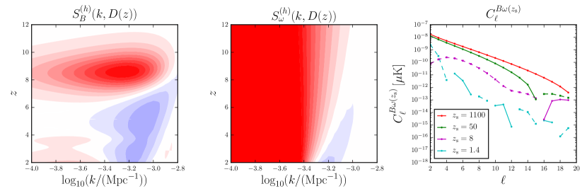
In the right panel of Fig. 1 we show the cross power spectrum $C_{l}^{B\omega(z_{\mathrm{s}})}$ for a set of source redshifts $z_{\mathrm{s}}$. This is the predicted signal in linear cosmological perturbation theory in a universe with gravitational waves. For the CMB case at $z_{\mathrm{s}}=1100$, this is the gravitational wave analog of the reionization-generated cross power spectrum $C_{\ell}^{E\phi(z_{\mathrm{s}})}$ between polarization $E$ modes and CMB lensing potential $\phi$ modes sourced by density fluctuations computed in Ref. Lewis et al. (2011).

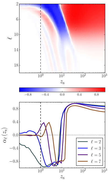
In Fig. 2 we show the cross-correlation coefficient, defined as

$$\alpha_{\ell}(z_{\mathrm{s}})=\dfrac{C_{\ell}^{B\omega(z_{\mathrm{s}})}}{\sqrt{C_{\ell}^{BB}C_{\ell}^{\omega\omega(z_{\mathrm{s}})}}}\,.$$ (11)

These two fields are strongly correlated for multipoles $\ell<20$, particularly for high-redshift sources.

Figure 3: Detection significance for correlation in the case of cosmic variance limited observations of both $B$ and $\omega(z_{\mathrm{s}})$ as a function of $z_{\mathrm{s}}$. Colored bands represent eras probed by different cosmological surveys. The plot suggests that the cross-correlation is best observed at higher redshifts, with the maximum signal situated around $z_{\mathrm{s}}\sim 50$. This curve is independent of the value of the tensor-to-scalar ratio, $r$. In principle, many redshift bins could be combined to significantly boost the total detectability.

V Detectability

We would like to estimate the cross-correlation between a (perhaps noisy) map of CMB $B$ modes and a reconstructed map of $\omega$ modes at some source redshift $z_{\mathrm{s}}$. Assuming full-sky data, for a given value of $\ell$ we could use the $2l+1$ pairs of observed spherical harmonic moments ($B_{\ell m}$, $\omega_{\ell m}$) to form the cross-correlation statistic

$$\hat{\rho}_{\ell}=\frac{\sum_{m}B_{\ell m}\omega_{\ell m}^{*}}{\sqrt{\sum_{m}|B_{\ell m}|^{2}\sum_{m^{\prime}}|\omega_{\ell m^{\prime}}|^{2}}}\,.$$ (12)

The estimator $\hat{\rho}_{\ell}$ can have a highly non-Gaussian distribution. For instance, in the limit where the experimental and reconstruction noises are very small and where the cross-correlation $\hat{\rho}_{\ell}$ becomes very close to 1, the values of $B_{\ell m}$ and $\omega_{\ell m}$ would become exactly equal (up to an overall multiplicative constant). The cross correlation would then be detectable at extremely high significance, even though the number of independent modes for a given $\ell$, namely $2\ell+1$, might not be large. In other words, this cross-correlation could in principle be detectable without being limited by cosmic variance.

To render the cross-correlation estimate more Gaussian, one can use the Fisher transformation Fisher (1915, 1921), given by

$$\hat{y}_{\ell}={1\over 2}\ln\left({1+\hat{\rho}_{\ell}\over 1-\hat{\rho}_{\ell}}\right)=\operatorname{atanh}(\hat{\rho}_{\ell})\,.$$ (13)

For $2l+1$ independent samples drawn from a bivariate Gaussian distribution in $(B_{\ell m},\omega_{\ell m})$, this transformed estimator has a nearly Gaussian distribution, with mean

$$\langle\hat{y}_{\ell}\rangle=\operatorname{atanh}\left(\frac{C_{\ell}^{B\omega(z_{\mathrm{s}})}}{\sqrt{\left(C_{\ell}^{BB}+N_{\ell}^{BB}\right)\left(C_{\ell}^{\omega\omega(z_{\mathrm{s}})}+N_{\ell}^{\omega\omega(z_{\mathrm{s}})}\right)}}\right)$$

$$\,.$$ (14)

and variance $\sigma_{\hat{y}_{\ell}}^{2}=1/(2\ell-2)$. Here, $C_{\ell}^{BB}$ and $C_{\ell}^{\omega\omega(z_{\mathrm{s}})}$ are the cosmological contributions to the variances in the $B_{\ell m}$ and $\omega_{\ell m}$ while the $N_{\ell}^{BB}$ and $N_{\ell}^{\omega\omega(z_{\mathrm{s}})}$ are the contributions from instrumental and reconstruction noise.

We take $N_{\ell}^{BB}$ to be a constant on the scales of interest, parameterized by a pixel noise level $N_{\ell}^{BB}=2(\Delta_{T})^{2}$. For $N_{\ell}^{\omega\omega(z_{\mathrm{s}})}$ we work in the flat-sky approximation and use the quadratic estimator of Ref. Hu and Okamoto (2002); Cooray et al. (2005) for the CMB, generalized to an intensity mapping survey with multiple redshift screens by Ref. Zahn and Zaldarriaga (2006):

$$\left(N_{\ell=|\mathbf{l}|}^{\omega\omega(z_{\mathrm{s}})}\right)^{-1} = \sum_{j=j_{\rm min}}^{j_{\rm max}}\frac{4}{|\mathbf{l}|^{4}}\int\frac{d^{2}\mathbf{l}^{\prime}}{(2\pi)^{2}}f_{\beta}^{j}(\mathbf{l}^{\prime},\mathbf{l}-\mathbf{l}^{\prime})F_{\beta}^{j}(\mathbf{l}^{\prime},\mathbf{l}-\mathbf{l}^{\prime}),$$

where $j$ indexes radial modes. For the CMB, which has only the $j=0$ term, we use the $\beta=EB$ quadratic estimator, with $f_{\beta}^{j}(\mathbf{l}_{1},\mathbf{l}_{2})=((\mathbf{l}_{1}+\mathbf{l}_{2})\times\mathbf{l}_{1})C_{\mathbf{l}_{1}}^{EE}\sin 2\varphi_{\mathbf{l}_{1},\mathbf{l}_{2}}$ and $F_{\beta}^{j}(\mathbf{l}_{1},\mathbf{l}_{2})=f_{\beta}^{j}(\mathbf{l}_{1},\mathbf{l}_{2})/C_{|\mathbf{l}_{1}|}^{EE,\mathrm{tot}}C_{|\mathbf{l}_{2}|}^{BB,\mathrm{tot}}$, where the $C_{|\mathbf{l}|}^{XX,\mathrm{tot}}$ denote the total power spectra including noise. For intensity mapping surveys, with $\beta=II$, we take $f_{\beta}^{j}(\mathbf{l}_{1},\mathbf{l}_{2})=(\mathbf{l}_{1}+\mathbf{l}_{2})\times(\mathbf{l}_{1}C_{\mathbf{l}_{1}}^{II}+\mathbf{l}_{2}C_{\mathbf{l}_{2}}^{II})$ and $F_{\beta}^{j}(\mathbf{l}_{1},\mathbf{l}_{2})=f_{\beta}^{j}(\mathbf{l}_{1},\mathbf{l}_{2})/2C_{|\mathbf{l}_{1}|}^{II,\mathrm{tot}}C_{|\mathbf{l}_{2}|}^{II,\mathrm{tot}}$.

One can then form the chi-square statistic with respect to the expectation for no correlation, using $\chi^{2}=\sum_{\ell}(\hat{y}_{\ell}/\sigma_{\hat{y}_{\ell}})^{2}$. For forecasting results for future data, we average over datasets, yielding

$$\langle\chi^{2}\rangle=\sum_{\ell}{(2\ell-2)}\langle\hat{y}_{\ell}\rangle^{2}\,,$$ (16)

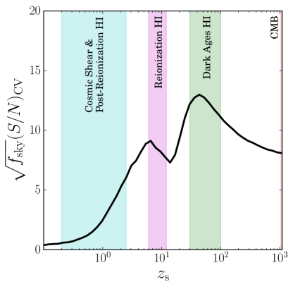
with $\langle\hat{y}_{\ell}\rangle$ given by Eq. (14). We compute $\langle\chi^{2}\rangle$ at a variety of source redshifts and for a range of noise levels $N_{\ell}^{BB}$ and $N_{\ell}^{\omega\omega(z_{\mathrm{s}})}$. We report the significance with which we can reject the null hypothesis of no cross-correlation $\sqrt{\chi^{2}}$, which we loosely refer to as $(S/N)$ in Figs. 3 and 4.

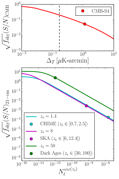
CMB ($z_{\mathrm{s}}\sim 1100$): For curl modes reconstructed using the CMB, we use the EB estimator, including iterative delensing of the scalar-induced $B$ modes Smith et al. (2012). Although yielding a lower noise level, using polarization rather than temperature for reconstruction actually reduces the overall $\omega$ signal by a factor of approximately 2 Dai (2014), which we have accounted for. In the top panel of Fig. 4, we show the significance with which the case of no correlation can be rejected, as a function of the survey noise in $\mu$K-arcmin. We have assumed that the $\omega$ map and the $B$ map are obtained from surveys with the same noise level; although the former can be obtained with a ground-based survey such as CMB-S4 Abazajian et al. (2016), the latter will require a nearly full-sky experiment to measure large scales (e.g. LiteBIRD Lit or CORE COR from space; CLASS CLASS collaboration (2016) from the ground). For very low noise levels of $\Delta_{T}\sim 0.17$ $\mu$K-arcmin, it might become difficult to distinguish curl modes from divergence modes Hirata and Seljak (2003). Even for noise levels $\Delta_{T}\sim 10^{-2}$ $\mu$K-arcmin, the cross-correlation is not detectable for $r=0.01$.

Figure 4: Top: Significance to reject the case of no correlation using only the CMB, as a function of the noise $\Delta_{T}$, assuming $r=0.01$.  The dashed curve indicates the noise level at which curl and convergence modes might not be distinguishable Hirata and Seljak (2003). Bottom: Significance for 21-cm surveys as a function of the curl-lensing reconstruction noise $N_{\ell}^{\omega\omega(z_{\mathrm{s}})}$, assuming $r=0.01$ and CMB noise $\Delta_{T}=0.25$ $\mu$K-arcmin for several ranges of source redshifts. Using multiple redshift screens can serve to reduce the noise $N_{\ell}^{\omega\omega(z_{\mathrm{s}})}$; for the three forecasted points shown, we sum over the given redshift range using the experimental configurations described in the text.

For our 21-cm forecasts, we assume that the CMB is mapped with $\Delta_{T}=0.25$ $\mu$K-arcmin and show results in Fig. 4 as a function of the curl lensing noise $N_{\ell}^{\omega\omega(z_{\mathrm{s}})}$ at various redshifts. The lensing reconstruction noise is in general a complicated function of antenna noise, configuration, baseline, frequency resolution, and bandwidth, but we simply assume a constant reconstruction noise at large scales in order to determine what is required to achieve a null rejection. We also show forecasts for a few specific experimental configurations described below.

Dark Ages ($30\leq z_{\mathrm{s}}\leq 100$): The 21-cm signal from the dark ages can be computed analytically Loeb and Zaldarriaga (2004); Bharadwaj and Ali (2004) and we will consider experimental limitations as in Ref. Chen et al. (2016). We assume that foreground cleaning will remove large-scale modes along the line of sight, which we take into account by setting $j_{\rm min}\geq 3$ as in Zahn and Zaldarriaga (2006); Pourtsidou and Metcalf (2014). We assume a 3 MHz bandwidth and a frequency resolution of $0.01$ MHz. Note that in practice the frequency resolution can easily be improved, however lensing reconstruction noise is typically most limited by the experimental baseline. We estimate the minimal baseline required to obtain a 3 sigma rejection of the null hypothesis given a tensor-to-scalar ratio $r=0.01$ and find that a baseline of $\sim 100$ km would suffice. Note that all we need is the lensing modes for $2\leq\ell\leq 20$. Our forecast is more realistic than Ref. Book et al. (2012), where the experiment under consideration was cosmic variance limited to $\ell=10^{6}$, which at $z=100$ translates to a baseline of $\sim 5000$ km. The points in the bottom panel of Fig. 4 are obtained by combining all independent redshifts to estimate the total noise reconstruction and assuming an average signal within our window.

Reionization ($6\leq z_{\mathrm{s}}\leq 12$): For a survey probing the reionization era Pen (2004), we consider a low-SKA type experiment to reconstruct the lensing noise through Eq. (LABEL:eq:lensingnoise). Basic experimental setup was taken from SKA while we compute the baseline density as a function of visibility $n(\mathbf{u})$ by considering a Gaussian distribution of detectors with $\sigma_{r}=700$m. We cut off the parallel modes at $j_{\rm max}=20$ and assume a bandwidth of 5 Mhz, with 21 redshift bins ($z_{\rm min}=6$, $z_{\rm max}=12.4$). From Fig. 4 it can be seen that one would need $N^{\omega\omega(z_{\mathrm{s}}}_{\ell}\leq 10^{-14}$ in order to obtain a 3$\sigma$ rejection of the null cross. Putting aside practical issues, we estimate that a post-SKA type experiment with a baseline of 100 km (instead of $\sim 1$ km) and the same antenna filling factor (i.e. $A_{\rm eff}=100A_{\rm eff}^{\rm SKA}$) would achieve such a reconstruction. We would like to stress that the signal peaks towards higher $z_{\mathrm{s}}$, which motivates a more detailed analysis of the signal in the redshift ranges $15\leq z_{\mathrm{s}}\leq 30$ ($z_{\rm max}^{\rm SKA}\sim 27$). Furthermore, lensing reconstruction relies sensitively on the smallest modes; optimal antenna distributions Greig et al. (2015) can be considered to measure exactly those modes. We will leave this for future work.

Post-Reionization ($0.5\leq z_{\mathrm{s}}\leq 2.5$): At the lowest redshifts we consider a CHIME-like experiment CHI . We assume 4 cylinders of 20 by 100 m with a total of 2048 detectors. We compute the visibility function $n(\mathbf{u})$ as in Ref. Xu et al. (2015). We assume an 80 MHz bandwidth, resulting in $\sim 5$ redshift bins in the range $0.7\leq z_{\mathrm{s}}\leq 2.5$ We estimate the 21-cm signal as in Ref. Shaw et al. (2014). Similar to lensing reconstruction using galaxies Dodelson (2010); Chisari et al. (2014), it would be very impractical to detect the cross-correlation in this redshift window. The reason is that based on Fig. 4 even in the most optimistic case, such a probe barely reaches the 3$\sigma$ threshold for null rejection. On the other hand, it is easier to observe small scale modes at low $z_{\mathrm{s}}$. Further investigation is needed to address whether a survey aimed at slightly higher redshifts, but with a much larger cylinder, could potentially push this towards the null rejection threshold.

VI Conclusion and Discussion

We considered the cross-correlation between CMB $B$-modes and curl-lensing modes for sources at various redshifts. Since both are sourced by primordial gravitational waves, evidence of non-zero cross-correlation would be a strong indication that observed $B$-modes are due to primordial gravitational waves rather than astrophysical foregrounds or systematics.

We showed that, for $\ell>2$, the cross-correlation has larger amplitude for sources at redshifts $z_{\mathrm{s}}\gtrsim 3$. This suggests that cosmic surveys aimed at mapping out higher redshifts, such as future 21-cm experiments, are much more sensitive to this cross-correlation than low redshift probes. Although the CMB provides the highest redshift screen available, the low noise required for lensing reconstruction in order to detect the cross-correlation with CMB data alone seems to be out of reach for the foreseeable future. The three-dimensional information available in 21-cm experiments allows for lower noise lensing reconstruction by combining many independent redshift slices.

We showed that in principle a post-SKA experiment aimed to detect the HI signal at redshifts $15\leq z\leq 30$ is potentially as capable of constraining this cross-correlation as much more futuristic surveys of the cosmic dark ages.

On a side note, another motivation to investigate this cross-correlation is that it could confuse a measurement of higher order correlation functions, searching for primordial tensor non-Gaussianity Meerburg et al. (2016).

We are currently entering the precision CMB polarization era, with the goal of detecting the tiny signatures left by primordial gravitational waves. Before we can confidently conclude that an observation of $B$-mode polarization on large angular scales was indeed sourced by primordial gravitational waves, we need to rule out the possibility of contamination by foregrounds or systematics. In this paper we showed that, although futuristic, the cross-correlation between CMB $B$-modes and curl lensing provides a useful test to establish the primordial nature of observed CMB $B$ modes.

Acknowledgments We would like to thank Cora Dvorkin, Gil Holder, Ue-Li Pen, and Harrison Winch for helpful discussions, and Scott Dodelson, Marc Kamionkowski, and David Spergel for comments on an early draft of this paper. J.M. was supported by the Vincent and Beatrice Tremaine Fellowship.

References

- Zaldarriaga and Seljak (1997) M. Zaldarriaga and U. Seljak, Phys. Rev. D55, 1830 (1997), arXiv:astro-ph/9609170 [astro-ph] .
- Kamionkowski et al. (1997) M. Kamionkowski, A. Kosowsky, and A. Stebbins, Physical Review Letters 78, 2058 (1997), astro-ph/9609132 .
- Kamionkowski and Kovetz (2015) M. Kamionkowski and E. D. Kovetz, (2015), 10.1146/annurev-astro-081915-023433, arXiv:1510.06042 [astro-ph.CO] .
- BICEP2 Collaboration et al. (2016) BICEP2 Collaboration, Keck Array Collaboration, P. A. R. Ade, et al., Physical Review Letters 116, 031302 (2016), arXiv:1510.09217 .
- (5) http://litebird.jp/eng.
- CLASS collaboration (2016) CLASS collaboration, ArXiv e-prints (2016), arXiv:1608.08234 [astro-ph.IM] .
- (7) http://www.core-mission.org.
- Abazajian et al. (2016) K. N. Abazajian et al., “CMB-S4 Science Book, First Edition,” (2016), arXiv:1610.02743 [2] .
- Alizadeh and Hirata (2012) E. Alizadeh and C. M. Hirata, Phys. Rev. D 85, 123540 (2012), arXiv:1201.5374 [astro-ph.CO] .
- Cooray et al. (2005) A. Cooray, M. Kamionkowski, and R. R. Caldwell, Phys. Rev. D 71, 123527 (2005), astro-ph/0503002 .
- Namikawa et al. (2015) T. Namikawa, D. Yamauchi, and A. Taruya, Phys. Rev. D91, 043531 (2015), arXiv:1411.7427 [astro-ph.CO] .
- Stebbins (1996) A. Stebbins, (1996), arXiv:astro-ph/9609149 [astro-ph] .
- Dodelson et al. (2003) S. Dodelson, E. Rozo, and A. Stebbins, Phys. Rev. Lett. 91, 021301 (2003), arXiv:astro-ph/0301177 [astro-ph] .
- Dodelson (2010) S. Dodelson, Phys. Rev. D 82, 023522 (2010), arXiv:1001.5012 .
- Li and Cooray (2006) C. Li and A. Cooray, Phys. Rev. D74, 023521 (2006), arXiv:astro-ph/0604179 [astro-ph] .
- Book et al. (2012) L. Book, M. Kamionkowski, and F. Schmidt, Phys. Rev. Lett. 108, 211301 (2012).
- Chisari et al. (2014) N. E. Chisari, C. Dvorkin, and F. Schmidt, Phys. Rev. D 90, 043527 (2014), arXiv:1406.4871 .
- Tram and Lesgourgues (2013) T. Tram and J. Lesgourgues, jcap 10, 002 (2013), arXiv:1305.3261 .
- Cooray and Hu (2002) A. Cooray and W. Hu, Astrophys. J. 574, 19 (2002), arXiv:astro-ph/0202411 [astro-ph] .
- Pratten and Lewis (2016) G. Pratten and A. Lewis, JCAP 1608, 047 (2016), arXiv:1605.05662 [astro-ph.CO] .
- Hirata and Seljak (2003) C. M. Hirata and U. Seljak, Phys. Rev. D68, 083002 (2003), arXiv:astro-ph/0306354 [astro-ph] .
- Schmidt and Jeong (2012) F. Schmidt and D. Jeong, Phys. Rev. D86, 083513 (2012), arXiv:1205.1514 [astro-ph.CO] .
- Lesgourgues (2011) J. Lesgourgues, ArXiv e-prints (2011), arXiv:1104.2932 [astro-ph.IM] .
- Ade et al. (2016) P. A. R. Ade et al. (Planck), Astron. Astrophys. 594, A13 (2016), arXiv:1502.01589 [astro-ph.CO] .
- Lewis et al. (2011) A. Lewis, A. Challinor, and D. Hanson, JCAP 1103, 018 (2011), arXiv:1101.2234 [astro-ph.CO] .
- Fisher (1915) R. A. Fisher, Biometrika 10, 507 (1915).
- Fisher (1921) R. A. Fisher, Metron. 1, 3 (1921).
- Lu and Pen (2008) T. Lu and U.-L. Pen, Mon. Not. Roy. Astron. Soc. 388, 1819 (2008), arXiv:0710.1108 [astro-ph] .
- Hu and Okamoto (2002) W. Hu and T. Okamoto, Astrophys. J. 574, 566 (2002), arXiv:astro-ph/0111606 [astro-ph] .
- Zahn and Zaldarriaga (2006) O. Zahn and M. Zaldarriaga, Astrophys. J. 653, 922 (2006), astro-ph/0511547 .
- Smith et al. (2012) K. M. Smith, D. Hanson, M. LoVerde, C. M. Hirata, and O. Zahn, JCAP 1206, 014 (2012), arXiv:1010.0048 [astro-ph.CO] .
- Dai (2014) L. Dai, Phys. Rev. Lett. 112, 041303 (2014), arXiv:1311.3662 [astro-ph.CO] .
- Loeb and Zaldarriaga (2004) A. Loeb and M. Zaldarriaga, Physical Review Letters 92, 211301 (2004), arXiv:astro-ph/0312134 .
- Bharadwaj and Ali (2004) S. Bharadwaj and S. S. Ali, mnras 352, 142 (2004), arXiv:astro-ph/0401206 .
- Chen et al. (2016) X. Chen, P. D. Meerburg, and M. Münchmeyer, JCAP 1609, 023 (2016), arXiv:1605.09364 [astro-ph.CO] .
- Pourtsidou and Metcalf (2014) A. Pourtsidou and R. B. Metcalf, Monthly Notices of the Royal Astronomical Society: Letters 439, L36 (2014).
- Pen (2004) U.-L. Pen, New Astronomy 9, 417 (2004), astro-ph/0305387 .
- (38) https://www.skatelescope.org/wp-content/uploads/2012/07/SKA-TEL-SKO-DD-001-1_BaselineDesign1.pdf.
- Greig et al. (2015) B. Greig, A. Mesinger, and L. V. E. Koopmans, ArXiv e-prints (2015), arXiv:1509.03312 .
- (40) http://chime.phas.ubc.ca.
- Xu et al. (2015) Y. Xu, X. Wang, and X. Chen, Astrophys. J. 798, 40 (2015), arXiv:1410.7794 .
- Shaw et al. (2014) J. R. Shaw, K. Sigurdson, U.-L. Pen, A. Stebbins, and M. Sitwell, The Astrophysical Journal 781, 57 (2014).
- Meerburg et al. (2016) P. D. Meerburg, J. Meyers, A. van Engelen, and Y. Ali-Haïmoud, Phys. Rev. D93, 123511 (2016), arXiv:1603.02243 [astro-ph.CO] .