Measurement of the Cold Dark Matter-Neutrino Dipole in the TianNu Simulation

Abstract

Measurements of neutrino mass in cosmological observations rely on two point statistics that are hindered by significant degeneracies with the optical depth and galaxy bias. The relative velocity effect between cold dark matter and neutrinos induces a large scale dipole into the matter density field and may be able to provide orthogonal constraints to standard techniques. We numerically investigate this dipole in the TianNu Simulation, which contains cold dark matter and 50 meV neutrinos. We first compute the dipole using a new linear response technique where we treat the displacement caused by the relative velocity as a phase in Fourier space and then integrate the matter power spectrum over redshift. Then, we compute the dipole numerically in real space using the simulation density and velocity fields. We find excellent agreement between the linear response and N-body methods. Utilizing the dipole as an observational tool will require two tracers of the matter distribution that are differently biased with respect to the neutrino density.

I Introduction

Terrestrial oscillation experiments have convincingly demonstrated that neutrinos are massive, and the measured mass splittings provide a lower bound on the neutrino mass scale: $M_{\nu}=\sum m_{\nu}\gtrsim 0.06$ eV Capozzi et al. (2016). The best upper bounds currently come from cosmological observations. The typical signature of cosmological neutrinos is a characteristic mass dependent suppression in the total matter power spectrum on small scales. This provides a conceptually simple way to infer the neutrino mass from two-point statistics: measure the amplitude of fluctuations on large scales using the cosmic microwave background (CMB) and compare it to the small scale amplitude inferred from large scale structure observations. For instance, Planck is sensitive to both the primary CMB (which depends on the scalar amplitude, $A_{S}$) and weak lensing of the CMB (which comes from smaller scale mass distributions), which yield a constraint of $M_{\nu}<0.23$ eV when combined Planck Collaboration et al. (2015). Alternatively, the small scale measurement can be taken from direct large scale structure observations. For example, combining Planck and Lyman-Alpha measurements from BOSS yield $M_{\nu}<0.12$ eV Palanque-Delabrouille et al. (2015).

A number of upcoming experiments are aiming to improve this measurement of $M_{\nu}$ with the goal of resolving all possible masses down to the minimal mass of $\sim 0.06$ eV. The Dark Energy Spectroscopic Instrument (DESI) is forecasted to have a mass resolution of $\sim 0.02$ eV Font-Ribera et al. (2014) as does the next generation CMB Stage IV (CMB S4) experiment when combined with DESI baryon acoustic oscillation (BAO) measurements Abazajian et al. (2016). However, significant challenges remain in utilizing the two point function due to a number of parameters that must be precisely controlled. The well known degeneracy between $A_{S}$ and the optical depth $\tau$ is still a consistent obstruction, and will hinder neutrino mass sensitivity in CMB S4 if the current measurement from Planck is not improved upon. On small scales, the limiting factor is disentangling the small neutrino effect from large and uncertain baryonic physics. To reach $0.02$ eV sensitivity, DESI must map its well resolved galaxy power spectrum to the underlying matter power spectrum which requires a highly precise knowledge of the galaxy bias. If this cannot be done, the DESI constraints with only BAO and Lyman-Alpha fall to $0.098$ eV.

There is therefore clear motivation to search for new techniques beyond the two point function that may depend less, or differently, on $\tau$, the galaxy bias, or baryonic astrophysics. A recent example of such a technique is differential neutrino condensation, which exploits fluctuations of the neutrino to CDM density ratio Yu et al. (2016). In a series of papers we have studied another probe of neutrino mass that utilizes the relative velocity between the neutrinos and CDM. In Zhu et al. (2014), a large scale CDM-neutrino dipole was predicted due to the displacement of initially concurrent regions of CDM and neutrino density. In Zhu et al. (2016), a second smaller scale effect was identified as arising due to dynamical friction on CDM halos moving through a more homogeneous neutrino background. Finally, Inman et al. (2015) implemented neutrinos in the N-body code CUBEP³M Harnois-Déraps et al. (2013) and measured the relative velocity under non-linear gravitational evolution. This relative velocity was also shown to be highly correlated with the underlying matter density field and can therefore be accurately predicted.

In this paper we utilize the TianNu simulation, described in §II, to compute the CDM-neutrino dipole in two different ways. In §III.1, we compute the dipole via an integral over the non-linear CDM power spectrum with the relative velocity contributing a phase shift in Fourier space. In §III.2, we perform the calculation in real space by displacing hierarchically averaged density and velocity fields. We find that the latter is significantly larger on all scales compared to the predictions in Zhu et al. (2014), but is well matched by the new response computation provided we take into account the relative velocity correlation scale.

II TianNu Simulation

The TianNu simulation is an N-body simulation containing both CDM and $50$ meV neutrino particles performed on the Tianhe-2 supercomputer Yu et al. (2016); Emberson et al. (2016). Simulations with neutrinos require compromise between two competing needs: sample variance and Poisson noise. On small scales, the large thermal motion of neutrinos causes them to be severely dominated by Poisson noise. This noise can be reduced through the use of a large number of particles and a smaller box size. On the other hand, the largest modes in the box will be limited by sample variance so the box cannot be too small. The TianNu simulation uses $6912^{3}$ CDM particles and $13824^{3}$ neutrino particles in a box of size $1200$ Mpc/h. This choice allows for scales $0.05<k/($h/Mpc$)<0.5$ to be relatively unafflicted from either form of noise.

In addition to the Poisson noise, the large thermal velocities also make simulating neutrinos difficult at high redshift. For our simulation, we evolve the CDM alone from redshift $100$ to $5$ and then inject neutrinos. The simulation is then evolved to redshift $0.01$.

For the dipole computation, we are interested in the CDM and neutrino density and velocity fields on relatively large scales. We compute $\delta_{c}$ and $\delta_{\nu}$ via the Nearest-Grid-Point method Hockney and Eastwood (1988). The relative velocity is the difference between the CDM and neutrino velocities: $\vec{v}_{c\nu}\equiv\vec{v}_{c}-\vec{v}_{\nu}$ computed by taking the average velocity of the particles in each cell. We compute the fields with only $576^{3}$ cells ($\sim 2.1$ Mpc/h per cell per dimension). This both reduces the necessary computational time as well as smoothes over small scale structure to improve the accuracy of the average velocity method.

Figure 1: Top. Cold dark matter-neutrino relative velocity power spectrum from the TianNu simulation (solid) and linear theory (dashed). TianNu fields are computed on a reduced $576^{3}$ mesh using the average particle velocity in each cell. Bottom. The corresponding correlation functions obtained by integrating the relative velocity power spectrum. The dotted vertical line is the simulation coherence length, the scale at which the correlation function drops to half its value.

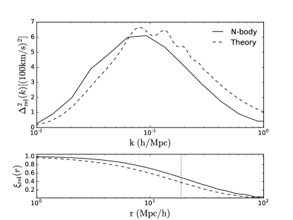
In the top panel of Fig. 1 we show the CDM-neutrino relative velocity power, $\Delta^{2}_{\text{rel}}(k)$. We find the N-body relative velocity to be slightly larger than that in Inman et al. (2015) (the black curve in Fig. 10), especially on large scales. This is likely due to the larger box size used ($1200$ Mpc/h versus $500$) which captures additional power from large scale modes. We compute the integrated relative velocity:

$$v_{r}=\sqrt{\int\Delta^{2}_{\rm rel}(k)\frac{dk}{k}}=392\ {\rm km}/{\rm s}.$$ (1)

We also compute the monopole correlation function:

$$\xi(r) =\int d^{3}kP(k)e^{(i\vec{k}\cdot\vec{r})}$$

$$=\int dkk^{2}P(k)/(2\pi^{2})j_{0}(kr)$$

$$\xi(r) \rightarrow\xi_{0}(r)/\xi_{0}(0)$$ (2)

with $P(k)$ being the monopole power spectrum, $\Delta^{2}(k)=\frac{k^{3}}{2\pi^{2}}P(k)$ and $j_{0}$ being the spherical Bessel function and the last line indicates that we divide by the $r=0$ value. This result is shown in the bottom panel of Fig. 1. The correlation length is defined as the scale at which $\xi(R_{\rm rel})=0.5$. We find $R_{\rm rel}=18.7$ Mpc/h in simulation, which is slightly larger than the linear value of $13.4$ Mpc/h.

III Dipole Correlation Function

III.1 Linear Response Dipole

In Zhu et al. (2014), the calculation of the dipole $P_{c\nu 1}$ was performed using Moving Background Perturbation Theory (MBPT). This approach, introduced in Tseliakhovich and Hirata (2010), solves the hydrodynamic Continuity and Euler Equations for CDM and neutrinos with the neutrinos having a constant sound speed proportional to their Fermi-Dirac dispersion. Here, we use a new technique for describing the relative velocity that uses the linear response solution for the neutrino density field. This allows for the full Fermi-Dirac distribution information to be utilized.

Formally, neutrinos obey the non-linear collisionless Vlasov equation although fluid approximations are also in common use. Once linearized, the Vlasov equations has an integral solution (see e.g. Ringwald and Wong (2004); Ali-Haïmoud and Bird (2013); Inman and Pen (2016) for additional discussions) of the form:

$$\delta_{\nu}=\frac{3}{2}H_{0}^{2}\Omega_{m}\int_{s_{i}}^{s}ds^{\prime}a(s-s^{\prime})\delta_{m}(k,s^{\prime})V(k(s-s^{\prime})/\beta)$$ (3)

where $s$ is a time-like variable ($ds=a^{2}dt$), $\delta_{m}\simeq\delta_{c}$ is the dominant density contrast and $\beta=m/(k_{B}Tc)$ encodes the relevant neutrino properties: mass $m$ and temperature $T=(4/11)^{1/3}2.725$ K. $V(x)$ is a function that encodes the neutrino’s initial relativistic Fermi-Dirac velocity distribution:

$$V(x)=\frac{\int dvv^{2}(\exp(v)+1)^{-1}j_{0}(xv)}{\int dvv^{2}(\exp(v)+1)^{-1}}.$$ (4)

The fluid approximation also has an integral solution with the same Eq. 3 but $V(x)=j_{0}(x*c_{s})$ where $c_{s}$ is the sound speed Inman and Pen (2016). We have verified that we are able to qualitatively reproduce the results in Zhu et al. (2014) using the fluid linear response method.

If neutrinos and CDM have a relative velocity $\vec{v}_{r}(z)$ that is coherent (i.e. independent of position $\vec{x}$), then the two species will flow past one another and become displaced $\vec{d}=\int\vec{v}_{r}(z)d\eta$ with $\eta$ the conformal time. Since our simulation starts at such a late redshift, we simplify the displacement and take a constant relative velocity $\vec{v}_{r}(z)\simeq\vec{v}_{r}\rightarrow\vec{d}(\eta)=\vec{v}_{r}(\eta-\eta_{i})$. In Fourier space, such a displacement leads to an additional phase, which we take to be in the CDM: $\delta_{c}(\vec{k})\rightarrow\delta_{c}(\vec{k})e^{-i\vec{k}\cdot\vec{d}}$. Hence, the cross power can be written as $P_{c\nu}=\langle\delta_{c}\tilde{\delta}_{\nu}\rangle$ with

$$\tilde{\delta}_{\nu}= \frac{3}{2}H_{0}^{2}\Omega_{m}\int_{s_{i}}^{s}ds^{\prime}a(s-s^{\prime})$$

$$\delta_{c}(k,s^{\prime})V(k(s-s^{\prime})/\beta)e^{-i\vec{k}\cdot(\vec{d}(\eta)-\vec{d}(\eta^{\prime}))}$$ (5)

with $\eta^{\prime}$ corresponding to $s^{\prime}$. If we define $\mu=\vec{k}\cdot\vec{d}/(kd)$ and expand the exponential factor $e^{-ikd\mu}\simeq 1-ikd\mu$ we obtain the dipole component of the power spectrum, $(-i\mu)P_{c\nu 1}(z,k,\mu)=-i\mu kv_{r}\langle\delta_{c}\tilde{\delta}_{\nu 1}\rangle$:

$$\tilde{\delta}_{\nu 1}= \frac{3}{2}H_{0}^{2}\Omega_{m}\int_{s_{i}}^{s}ds^{\prime}a(s-s^{\prime})$$

$$\delta_{c}(k,s^{\prime})V(k(s-s^{\prime})/\beta)(\eta-\eta^{\prime})$$ (6)

where we have factored out the generic contributions of $\mu$, $v_{r}$ and $k$ from the integral. For comparison with our numerical computation, we look for the antisymmetric combination: $P_{c\nu 1}(\mu)-P_{c\nu 1}(-\mu)$ which is twice that of Eq. III.1.

Figure 2: Cold dark matter (blue) and neutrino (red) auto and cross (green) power spectra in the TianNu simulation. Solid curves are computed directly from the density fields. Dotted curves are computed via the CLASS Boltzmann code. Dashed curves utilize linear response. The dipole cross power spectrum is shown in purple. The straight line $\propto k^{3}$ and shown in dark grey is the neutrino Poisson noise. The shaded grey region is the sample variance due to the simulation box size.

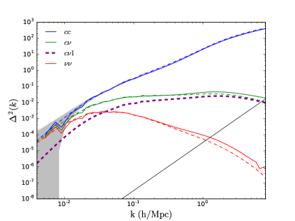
We plot power spectra in Fig. 2. Solid lines are those computed from the TianNu simulation: blue is CDM, red is neutrino and green is the cross power. Dashed curves are those from the linear response calculations described before, taking $\delta_{c}$ to be the square root of the HaloFit power spectrum $P_{HF}$ Smith et al. (2003). Dotted curves are computed from the CLASS code Blas et al. (2011) assuming $P_{ij}=P_{HF}\frac{T_{i}T_{j}}{T_{m}^{2}}$ with $T_{i}$ being the linear transfer functions. The filled grey region surrounding the HALOFIT power shows the sample variance of the simulation. The dark grey curve crossing the neutrino spectrum is the Poisson noise (which we have subtracted out from the simulation neutrino power). We see that there is a relatively noise free region as discussed earlier in §II.

The dipole correlation function is given by the Fourier transform of the dipole power spectrum:

$$\xi_{1}(r) =\int d^{3}k(-i\mu)P_{1}(k)e^{i\vec{k}\cdot\vec{r}}$$

$$=\int dkk^{2}P_{1}(k)/(2\pi^{2})j_{1}(kr)$$ (7)

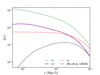
where $j_{1}(kr)$ is another spherical Bessel function. In order to prevent ringing on large scales, we include a Gaussian cutoff, $\exp[-(k/(0.75\mbox{h}/\mbox{Mpc}))^{2}]$, in the integral; since this cutoff suppresses power on small scales, we apply a high pass filter in $r$ to smoothly turn the cutoff on around $r\sim 7.5$Mpc/h. We perform this integral numerically and show the results in Fig. 3. We find significant enhancement on small scales compared to Zhu et al. (2014) indicating that there is additional clustering that should be taken into account.

Figure 3: Correlation functions computed using the linear response method. The green curve is the cold dark matter-neutrino cross correlation. Red is the neutrino auto correlation function. Purple is the dipole correlation function. The black curve is reproduced from Zhu et al. (2014) which approximated neutrinos as a perfect fluid with constant sound speed.

III.2 Numerical Dipole

There are many ways to compute correlation functions Zhang and Pen (2005). We compute correlation functions in real space, using the method of hierarchical grids. We first displace the grids and then multiply their elements. This can be done in each direction (6 total displacements coresponding to $\pm x,\pm y,$ or $\pm z$), in each pair of directions (12 total displacements, e.g. $+x+y,-x+y,-x-y,+x-y$ and permutations with $z$) and for all three directions (8 total displacements, e.g. the four pairs of displacements discussed before with $\pm z$ included). After this, we average our grids down by a factor of two and repeat. This algorithm is straightforward to parallelize which we have done with MPI, although it is not necessary for the computations here. We note that averaging the grid to obtain larger displacements can cause a small amount of artifacting (after every third point). This could be resolved by displacing the fields further rather than averaging, but this requires a significantly larger computational cost.

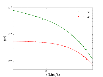
We first compute the monopole correlation functions to validate our algorithm. These results are shown in Fig. 4 alongside the linear response predictions. We find excellent agreement at all scales as is expected.

Figure 4: The monopole neutrino auto correlation function (red) and CDM-neutrino cross correlation function (green). Dots are computed numerically in real space. Lines are reproduced from Fig. 3 for comparison.

We now describe the computation of the dipole directly from the TianNu simulation. The relative velocity becomes a function of position, $\vec{v}_{\rm rel}(\vec{x})$, and we must now consider a three point correlation function:

$$\xi_{c\nu 1}=\langle\delta_{c}(\vec{x})\delta_{\nu}(\vec{x}+\vec{r})\hat{v}_{\rm avg}(\vec{x},\vec{x}+\vec{r})\cdot\hat{r}\rangle$$ (8)

where we have the freedom to choose the functional dependence of $\hat{v}_{\rm avg}$ on $\vec{x}$ and $\vec{r}$ as is convenient. Since we expect the relative velocity to be coherent on scales $r<R_{\rm rel}$, we simply take the average value of the relative velocity at both $\vec{x}$ and $\vec{x}+\vec{r}$. To see that this yields a dipole, consider the transformation $\vec{r}\rightarrow-\vec{r}$ and the change of variables $\vec{x}\rightarrow\vec{x}-\vec{r}$. Since $\hat{v}_{\rm avg}(\vec{x},\vec{x}+\vec{r})=\hat{v}_{\rm avg}(\vec{x}+\vec{r},\vec{x})$, the correlation function then becomes $\langle\delta_{c}(\vec{x}+\vec{r})\delta_{\nu}(\vec{x})\hat{v}_{\rm avg}(\vec{x}+\vec{r},\vec{x})\cdot(-\hat{r})\rangle$. If we average this result with Eq. 8, we obtain the antisymmetric CDM-neutrino dipole correlation function, $\xi_{c\nu 1}$, in the direction of the relative velocity, as:

$$\xi_{c\nu 1}(r)=\frac{1}{2}\langle\left[\delta_{c}(\vec{x})\delta_{\nu}(\vec{x}+\vec{r})-\delta_{\nu}(\vec{x})\delta_{c}(\vec{x}+\vec{r})\right]\hat{v}_{\rm avg}\cdot\hat{r}\rangle$$ (9)

with

$$\vec{v}_{\rm avg}=\frac{1}{2}\left(\vec{v}_{c\nu}(\vec{x})+\vec{v}_{c\nu}(\vec{x}+\vec{r})\right)$$ (10)

where it is understood we should only displace our fields in one direction. We see that generic CDM effects must cancel due to the antisymmetric combination of density fields. In other words, “$\xi_{cc1}$”$=0$. Furthermore, correlations orthogonal to the relative velocity do not contribute.

Figure 5: Top. Cold dark matter-neutrino dipole correlation functions. The dots are computed using hierarchical grid displacements of density and velocity fields. The dashed curve is computed using linear response. The solid curve is the linear response multiplied by the velocity correlation function (black curve in lower panel). Bottom. Relative velocity correlation function. The dots are computed using hierarchical grid displacements. The solid curve is computed as the Fourier transform of the relative velocity power spectrum. Both are normalized by their $r=0$ value. The dashed vertical line indicates the half-max velocity correlation length of $18.7$ Mpc/h.

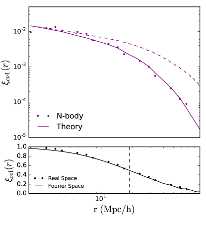
We show the CDM-neutrino dipole in the direction of the relative velocity as the purple points in the upper panel of Fig. 5. In addition we show the response dipole of Fig. 3 in dashed purple. On the largest scales there is some disagreement. This is not a surprise: the MBPT approximation assumes a coherent flow over the entire box. In reality, it is only coherent to scales $r\lesssim R_{\rm rel}$ and we therefore expect a smaller signal at distances larger than the coherence length. Fortunately, the information on the coherency of the relative velocity is precisely the relative velocity correlation function, $\xi_{\rm rel}(r)$, which we show in the lower panel of Fig. 5. Thus, by multiplying the MBPT prediction by $\xi(r)$ we obtain the solid purple curve in the upper panel of Fig. 5 which matches simulations remarkably well.

IV Discussion and Conclusion

We have demonstrated that the CDM-neutrino dipole exists and is well predicted via linear response for $50$ meV mass neutrinos. However, the real space computation performed here relies on knowing both the neutrino density and relative velocity. In Inman et al. (2015) it was demonstrated that the relative velocity direction is predictable with either a CDM or halo density field. In fact, the neutrino density field is also predictable Yu et al. (2016). However, this is assuming you know the transfer function. For a massive neutrino universe this transfer function can be computed from a Boltzmann code; however, for a massless neutrino Universe it is zero. Hence, while we can predict both the relative velocity and neutrino density at the same time, this does not result in an observable quantity.

In Zhu et al. (2014), the proposed observable was to use two distinct tracers of the density field that are differentially biased with respect to neutrinos. For instance, halos (observed via proxy galaxies) above and below a certain mass. A second option would be the lensing field (which depends on the linear sum of CDM and neutrino densities) and a galaxy survey (which depends primarily on CDM). We intend to investigate this in subsequent works.