Stationary Scalar Clouds Around Maximally Rotating Linear Dilaton Black Holes

Abstract

We investigate the wave dynamics of a charged massive scalar field propagating in a maximally rotating (extremal) linear dilaton black hole geometry. We prove the existence of a discrete and infinite family of resonances describing non-decaying stationary scalar configurations (clouds) enclosing these rapidly rotating black holes. The results obtained signal the potential stationary scalar field distributions (dark matter) around the extremal linear dilaton black holes. In particular, we analytically compute the effective heights of those clouds above the center of the black hole.

I Introduction

According to the “no-hair conjecture” Wheeler ; Book1 ; Hod1 , which is one of the milestones in understanding the subject of black hole (BH) physics Book2 ; Book3 , BHs are fundamental objects like the atoms in quantum mechanics, and they should be characterized by only 3-parameters: mass, charge, and angular momentum. In fact, the no-hair conjecture has an oversimplified physical picture: all residual matter fields for a newly born BH would either be absorbed by the BH or be radiated away to spatial infinity (this scenario excludes the fields having conserved charges) Hod1 ; BekT2 ; HodSr ; Her1 ; Her2 . In accordance with the same line of thought, other no-hair theorems indeed omitted static spin-$0$ fields sp01 ; sp02 ; sp03 ; sp04 ; sp05 , spin-$1$ fields sp11 ; sp12 ; sp13 ; sp14 , and spin-$\frac{1}{2}$ fields sph1 ; sph2 from the exterior of stationary BHs. On the other hand, significant developments in theoretical physics has led to other types of “hairy” BH solutions. A notable example is the colored BHs in Refs. CBH1 ; CBH2 . In addition to mass, for full characterization, a colored BH needs an additional integer number (independent of any conserved charge) which is assigned to the nodes of the Yang-Mills field. Other hairy BHs include different types of exterior fields that belong to the Einstein-Yang-Mills-Dilaton, Einstein-Yang-Mills-Higgs, Einstein-Klein-Gordon, Einstein-Skyrme, Einstein-Non-Abelian-Proca, Einstein-Gauss-Bonnet etc. theories (see for example, HBH17 ; HBH172 ; HBH173 ; HBH1 ; HBH2 ; HBH3 ; HBH4 ; HBH5 ; HBH6 ; HBH7 ; HBH8 ; HBH9 ; HBH10 ; HBH11 ; HBH12 ; HBH13 ; HBH14 ; HBH15 ; HBH16 ; HBH18 ; HBH19 ; HBH20 ; Bernard ).

Interestingly, many no-hair theories BekT2 ; sp13 ; sp14 ; sph1 ; sph2 ; NH1 ; NH4 ; NH6 ; NH7 ; NH8 do not cover the time-dependent field configurations surrounding the BH. Astronomical BHs are not tiny and unstable, but very heavy, large, and practically indestructible. Observations show that in the densely populated center of most galaxies, including ours, there are monstrous BHs GALAXY , which are many hundreds of millions of times heavier than the sun. As was shown in Barro , the regular time-decaying scalar field configurations surrounding a supermassive Schwarzschild BH do not fade away in a short time (according to the dynamical chronograph governed by the BH mass). Besides, ultra-light scalar fields are considered as a possible candidate for the dark matter halo (see for instance, Barro ; DM1 ; DM2 ; DM3 ).

Hod HodSr extended the outcomes of Barro to the Kerr BH, which is well-suited for studying astrophysical wave dynamics. Hod proved the presence of an infinite family of resonances (discrete) describing non-decaying (stationary) scalar configurations surrounding a maximally rotating Kerr BH. Thus, contrary to the finite lifetime of the static regular scalar configurations mentioned in Barro , the stationary and regular scalar field configurations (clouds) surrounding the realistic rotating BH (Kerr) survive infinitely long HodSr . To this end, Hod considered the dynamics of massive Klein-Gordon equation in the Kerr geometry. Moreover, the effective heights of those clouds above the center of the BH were analytically computed. The obtained results support the lower bound conjecture of Núñiez, et al. NH6 .

In line with the study by HodSr , the purpose of the present study is to explore the stationary and regular scalar field configurations surrounding maximally rotating linear dilaton BH (MRLDBH) Clement . These BHs have a non-asymptotically flat structure, similar to our universe model: Friedmann-Lemaître-Robertson-Walker spacetime universe . Rotating linear dilaton BHs are the solutions to the Einstein-Maxwel-dilaton-axion theory Leygnac . These BHs include dilaton and axion fields, which are canditates for the dark matter halo. Some current experiments are focused on the relationship between the dark matter and the dilaton and axion fields exp1 ; exp2 ; exp3 ; exp4 . Various studies have also focused on the rotating linear dilaton BHs rbh0 ; ldbh1 ; ldbh2 ; ldbh3 ; ldbh4 ; ldbh5 . In particular, the problem of area quantization (see area  for the insights of the famous Bekenstein’s area conjecture) from boxed quasinormal modes, which are obtained from caged massless scalar clouds, has been recently studied in ldbh4 . Our present study considers the charged massive Klein-Gordon-Fock (KGF) equation Klein ; Gordon ; Fock in the MRLDBH geometry. Thus, we investigate wave dynamics in that geometry and seek for the existence of possible resonances describing the stationary charged and massive scalar field configurations surrounding the MRLDBH.

This paper is organized as follows. In Sec. II, we review the rotating linear dilaton BHs with their characteristic properties and study the charged scalar field perturbation in this geometry. In Sec. III, we explore the existence of a discrete family of resonances describing stationary scalar configurations surrounding MRLDBH, and in sequel we compute the effective heights of those scalar configurations above the central MRLDBH. Finally, we provide conclusions in Sec. IV. We use the natural units with $c=G=k_{B}=\hbar=1$.

II Rotating linear dilaton BH spacetime and separation of KGF equation

In this section, we consider a charged massive scalar field coupled to a rotating linear dilaton BH. For a comprehensive analytical study, the rotating linear dilaton BH is assumed to be extremal, which requires the equality of mass term ($M$) with the rotation term ($a$). Namely, we focus on the case of a charged massive test scalar field in the geometry of MRLDBH spacetime.

The action of the Einstein-Maxwell-dilaton-axion theory is given by Leygnac

$$S=\frac{1}{16\pi}\int\sqrt{\left|g\right|}\left\{R-\frac{1}{2}e^{-4\phi}\partial_{\mu}\aleph\partial^{\mu}\aleph-2\partial_{\mu}\phi\partial^{\mu}\phi-\aleph F_{\mu\nu}\widetilde{F}^{\mu\nu}-e^{-2\phi}F_{\mu\nu}F^{\mu\nu}\right\}d^{4}x,$$ (1)

where $R$ is the Ricci scalar, $F_{\mu\nu}$ denotes the Maxwell tensor (antisymmetric rank-2 tensor field), and $\widetilde{F}^{\mu\nu}$ represents the dual of $F_{\mu\nu}$. Besides, $\phi$ and $\aleph$ are the dilaton field and the axion field (pseudoscalar), respectively. The metric solution to action (1) is designated with the rotating linear dilaton BH Clement , which is described in the Boyer-Lindquist coordinates as follows:

$$ds^{2}=-f(r)dt^{2}+\frac{dr^{2}}{f(r)}+h(r)\left[d\theta^{2}+\sin^{2}\theta\left(d\varphi-\frac{a}{h(r)}dt\right)^{2}\right].$$ (2)

The metric functions are given by

$$h(r)=rr_{0},$$ (3)

$$f(r)=\frac{Z}{h(r)},$$ (4)

where the constant parameter $r_{0}$ is directly proportional to the background electric charge $Q$: $r_{0}=\sqrt{2}Q$. In Eq. (4), $Z=\left(r-r_{2}\right)\left(r-r_{1}\right)$, where, $r_{1}$ and $r_{2}$ are the two positive roots of the condition of $f(r)=0$. In fact, $r_{1}$ and $r_{2}$ radii represent the inner and outer horizons, respectively. The explicit forms of those radii are given by

$$r_{1}=M-\sqrt{M^{2}-a^{2}},$$ (5)

$$r_{2}=M+\sqrt{M^{2}-a^{2}}.$$ (6)

In fact, $M$ is an integration constant in deriving the rotating linear dilaton BH solution. It is twice the quasilocal mass $M_{QL}$ BROWN-YORK of this non-asymptotically flat BH: $M=2M_{QL}$. The rotation parameter $a$ is related with the angular momentum ($J$) of the rotating linear dilaton BH via $a=\frac{\sqrt{2}J}{Q}$. Meanwhile, it is obvious from Eqs. (5) and (6) that having a BH solution, one should impose the condition of $M\geq a$. Thus, MRLDBH geometry corresponds to $a=M$.

The dilaton and axion fields are governed by Clement

$$e^{-2\phi}=\frac{h\left(r\right)}{r^{2}+a^{2}\cos^{2}\theta},$$ (7)

$$\aleph=-\frac{\sqrt{2}Qa\cos\theta}{r^{2}+a^{2}\cos^{2}\theta}.$$ (8)

Moreover, the electromagnetic 4-vector potential is given by

$$A^{em}=\frac{1}{\sqrt{2}}\left(e^{-2\phi}dt+a\sin^{2}\theta d\varphi\right).$$ (9)

The Hawking temperature WALD ; ROVELLI of the rotating linear dilaton BH can be obtained from the definition of surface gravity $\kappa$, as follows:

$$T_{H}=\frac{\kappa}{2\pi}=\frac{1}{4\pi}\left.\frac{df(r)}{dr}\right|_{r=r_{2}}=\frac{r_{2}-r_{1}}{4\sqrt{2}Q\pi r_{2}}.$$ (10)

As can be seen from Eq. (10), in the case of maximal rotation ($M=a\rightarrow r_{1}=0$: the extreme case), the rotating linear dilaton BH emits radiation with a constant temperature (since $Q$ possesses a fixed value), which is independent from the mass: $T_{H}=\left(4\sqrt{2}\pi Q\right)^{-1}$. Such a radiation is nothing but the well-known isothermal process in the subject of the thermodynamics. If $A_{H}$ stands for the surface area of the event horizon of the rotating linear dilaton BH, then the entropy of this BH is given by

$$S_{BH}=\frac{A_{H}}{4}=\sqrt{2}\pi Qr_{2}.$$ (11)

Angular velocity of the rotating linear dilaton BH is expressed as

$$\Omega_{H}=-\left.\frac{g_{tt}}{g_{t\varphi}}\right|_{r=r_{2}}=\frac{J}{Q^{2}r_{2}}.$$ (12)

Thus, the first law of thermodynamics of the rotating linear dilaton BH is evincible through the following differential equation

$$dM_{QL}=T_{H}dS_{BH}+\Omega_{H}dJ.$$ (13)

It is worth noting that Eq. (13) does not involve the electrostatic potential $\Phi_{e}$ GenThrm since $Q$ represents the fixed background charge Clement .

The dynamics of a charged massive scalar field $\Psi$ in the rotating linear dilaton BH spacetime is governed by the KGF equation (see for example, GOHAR ):

$$\left(\partial_{\mu}-iqA_{\mu}^{em}\right)\left(\sqrt{-g}g^{\mu\nu}\left(\partial_{\nu}-iqA_{\nu}^{em}\right)\Psi\right)-\sqrt{-g}\mu^{2}\Psi=0,$$ (14)

where $q$ and $\mu$ are the charge and mass of the scalar particle, respectively. We assume the ansatz for $\Psi,$ as follows:

$$\Psi\equiv\Psi_{lm}\left(t,r,\theta,\varphi\right)=e^{im\varphi}S_{lm}(\theta)R_{lm}(r)e^{-i\omega t},$$ (15)

where $\omega$ is the conserved frequency of the mode, and $l$ and $m$ are the spheroidal and azimuthal harmonic indices, respectively, with $-l\leq m\leq l$. In Eq. (15), $R_{lm}$ and $S_{lm}$ are the functions of radial and angular equations of the confluent Heun differential equation with the separation constant $\lambda_{lm}$ Heun ; Heun1 ; Iz2016 .

For the MRLDBH spacetime ($M=a$), the angular part of Eq. (14) obeys the following differential equation of spheroidal harmonics $S_{lm}(\theta)$ ABRAM ; TEU ; TEU2 :

$$\frac{1}{\sin\theta}\frac{\partial}{\partial\theta}\left(\sin\theta\frac{\partial S_{lm}}{\partial\theta}\right)+\left[\lambda_{lm}-\left(\frac{1}{2}\widehat{q}M\sin\theta\right)^{2}-\frac{m^{2}}{\sin^{2}\theta}\right]S_{lm}=0.$$ (16)

where $\widehat{q}=\sqrt{2}q.$ The above differential equation has two poles at $\theta=0$ and $\theta=\pi$. For a physical solution, $S_{lm}$ functions are required to be regular at those poles. This remark enables us to obtain a discrete set of eigenvalues $\lambda_{lm}$. In Eq. (16), $\frac{1}{2}M^{2}q^{2}\cos^{2}\theta$ can be treated as a perturbation term on the generalized Legendre equation ABRAM . Thus, we obtain the following perturbation expansion:

$$\lambda_{lm}-\left(\frac{1}{2}\widehat{q}M\right)^{2}=\sum_{k=0}^{\infty}c_{k}\left(-1\right)^{k}\left(\frac{1}{2}\widehat{q}M\right)^{2k}.$$ (17)

It is worth noting that in Ref. ABRAM , the expansion coefficients in the summation symbol of Eq. (17), $\left\{c_{k}\left(l,m\right)\right\},$ are explicitly given.

The radial equation of the KGF equation (14) in the MRLDBH geometry acts as a Teukolsky equation TEU ; TEU2 :

$$\Delta^{2}\frac{d}{dr}\left(\Delta^{2}\frac{dR_{lm}}{dr}\right)+\left\{\mathcal{H}^{2}-mM\left[2\widehat{q}Mr-mM+2h\left(r\right)\omega\right]-\Delta^{2}\left(K+h\left(r\right)\mu^{2}\right)\right\}R_{lm}=0,$$ (18)

where

$$\Delta=r-M,$$ (19)

and

$$\mathcal{H}=h\left(r\right)\omega+\frac{\widehat{q}}{2}\left(r^{2}+M^{2}\right).$$ (20)

For the MRLDBH, the event horizon is located at $r_{EH}=M,$ which is the degenerate zero of Eq. (19).

In general (for asymptotically flat BHs), the bound nature of the scalar clouds obey the following boundary conditions: purely ingoing waves at the event horizon and decaying waves at spatial infinity DDR ; SDet ; Dola ; HodB1 ; HodB2 . However, when we study the limiting behaviors of the radial equation (18), we get

$$R_{lm}\sim\begin{cases}\frac{1}{\sqrt{r}}BesselJ(0,qe^{\frac{r^{\ast}}{r_{0}}})\approx\frac{1}{\sqrt{q}r}\sin\left(qe^{\frac{r^{\ast}}{r_{0}}}\right)&\text{ as }r\rightarrow\infty\ \ (r^{\ast}\rightarrow\infty),\\ \frac{1}{\sqrt{r_{EH}}}e^{-i\left[\omega-\left(m-\widehat{q}M\right)\widetilde{\Omega}\right]r^{\ast}}&\text{ as }r\rightarrow r_{EH}\ r^{\ast}\rightarrow-\infty),\end{cases}$$ (21)

where $\widetilde{\Omega}=\left(r_{0}\right)^{-1}$ is the angular velocity of $r_{EH},$ and $r^{\ast}$ is the tortoise coordinate of the MRLDBH:

$$r^{\ast}=\int\frac{rr_{0}dr}{\Delta^{2}}=r_{0}\ln\left(\frac{\Delta}{\sqrt{2}}\right)-\frac{Mr_{0}}{\Delta}.$$ (22)

It is clear from the asymptotic solution (21) that unlike the Kerr BH HodSr , there are no decaying (bounded) waves in MLRDBH geometry at spatial infinity. Instead of this, we have oscillatory but fading waves (because of the factor $\frac{1}{r}$) at the asymptotic region [see Fig. (1)]. This result probably originates from the non-asymptotically flat structure of the MRLDBH geometry.

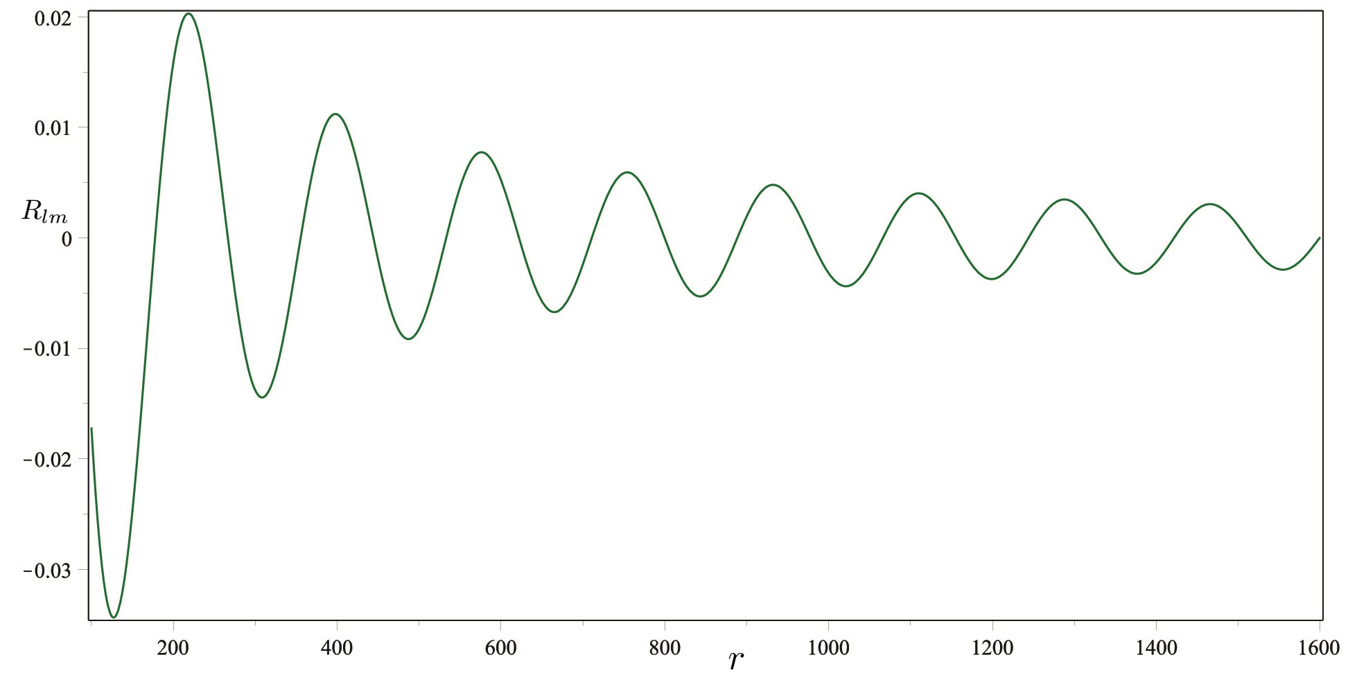
Figure 1: Asymptotic behavior of radial function $R_{lm}(r)$. The plot is governed by Eq. (21). The physical parameters are choosen as $M=1$, $q=0.05$, and $r_{0}=0.5$.

On the other hand, a very recent study confine has shown that scalar clouds can have a semipermeable surface, and thus they might serve as a “partial confinement” in which only outgoing waves are allowed to survive at the spatial infinity. Considering this fact, we will impose a particular asymptotic boundary condition to those non-decaying (unbounded) scalar clouds: only pure outgoing waves propagate at spatial infinity.

III Stationary resonances and effective heights of the scalar clouds

Stationary resonances or the so-called marginally stable modes are the stationary regular solutions of the KGF equation (14) around the horizon. They are characterized by $Im\left(\omega\right)=0$ HodSr , which corresponds to $\omega=\left(m-\widehat{q}M\right)\widetilde{\Omega}$ for the MRLDBH spacetime. In fact, such resonances saturate the superradiant condition Clement .

Introducing a new dimensionless variable

$$x=\frac{\Delta}{M},$$ (23)

one can see that the radial equation (18) can be rewritten as

$$x^{2}\frac{d^{2}R_{lm}}{dr^{2}}+2x\frac{dR_{lm}}{dr}+V_{eff}R_{lm}=0,$$ (24)

in which the effective potential is given by

$$V_{eff}=\left(\frac{1}{2}\widehat{q}Mx\right)^{2}+M\left(1+x\right)\left(m\widehat{q}-r_{0}{\mu}^{2}\right)+{m}^{2}-\lambda.$$ (25)

Letting

$$Y=xR_{lm}\text{ \ \ and \ \ }z=-i\widehat{q}Mx,$$ (26)

equation (24) transforms into the following differential equation

$$\frac{d^{2}Y}{dz^{2}}+\left(-\frac{1}{4}+\frac{\sigma}{z}+\frac{\frac{1}{4}-\beta^{2}}{z^{2}}\right)Y=0,$$ (27)

with

$$\sigma=i\left(m-\frac{r_{0}}{\widehat{q}}\mu^{2}\right)\text{ and }\beta^{2}=\lambda_{lm}+\frac{1}{4}-m^{2}+\left(r_{0}\mu^{2}-m\widehat{q}\right)M.$$ (28)

Without loss of generality, one can assume that $\beta$ is a non-negative real number HodSr . Therefore, Eq. (27) corresponds to a Whittaker equation ABRAM , whose solutions can be expressed in terms of the confluent hypergeometric functions $\mathcal{M}(a,b,z)$ ABRAM ; OLVER . Thus, the solution of Eq. (24) can be given by

$$R_{lm}=\frac{e^{-\frac{1}{2}z}}{\sqrt{z}}\left[C_{1}z^{\beta}\mathcal{M}\left(\frac{1}{2}+\beta-\sigma,1+2\beta,z\right)+C_{2}z^{-\beta}\mathcal{M}\left(\frac{1}{2}-\beta-\sigma,1-2\beta,z\right)\right],$$ (29)

where $C_{1}$ and $C_{2}$ are the integration constants. In the vicinity of the horizon, solution (29) reduces to MOR

$$R_{lm}\longrightarrow C_{1}z^{-\frac{1}{2}+\beta}+C_{2}z^{-\frac{1}{2}-\beta}.$$ (30)

Since the near horizon solution ($z\rightarrow 0$) must admit the regularity, one can figure out that

$$C_{2}=0\text{ and }\beta\geq\frac{1}{2}.$$ (31)

By using the asymptotic behaviors of the confluent hypergeometric functions ABRAM ; OLVER , for $z\rightarrow\infty,$ Eq. (29) can be approximated to

$$R_{lm}\longrightarrow C_{1}\left[e^{{\frac{1}{2}}z}{\frac{{\Gamma(1+2\beta)}}{{\Gamma({\frac{1}{2}}+\beta-\sigma)}}}z^{-1-\sigma}+e^{-{\frac{1}{2}}z}{\frac{{\Gamma(1+2\beta)}}{{\Gamma({\frac{1}{2}}+\beta+\sigma)}}}z^{-1+\sigma}(-1)^{-{\frac{1}{2}}-\beta+\sigma}\right].$$ (32)

Recalling the complex structure of $z$ [see Eq. (26)], we infer that the first term in the square bracket of Eq. (32) stands for the asymptotic ingoing waves, however the second one represents the asymptotic outgoing waves. According to the physical boundary conditions aforementioned, the asymptotic ingoing wave $\left(\sim e^{{\frac{1}{2}}z}\right)$ in Eq. (32) must be terminated. This is possible by employing the pole structure of the Gamma function ($\Gamma(\tau)$ has the poles at $\tau=-n$ for $n=0,1,2,...$ABRAM ). Therefore, the resonance condition for the stationary unbound states of the field eventually becomes

$$\frac{1}{2}+\beta-\sigma=-n.$$ (33)

It is convenient to express the radial solution of the unbound states in a more compact form by using the generalized Laguerre polynomials $L_{n}^{\left(2\beta\right)}\left(z\right)$ ABRAM :

$$R_{lm}=C_{1}z^{-\frac{1}{2}+\beta}e^{-{\frac{1}{2}}z}L_{n}^{\left(2\beta\right)}\left(z\right).$$ (34)

One can deduce from the resonance condition (33) that ${\sigma}$ should be a real number. However, taking cognizance of Eq. (28), which indicates that ${\sigma}$ is a pure imaginary parameter, we conclude that the resonances correspond to ${\sigma=0}$. Thus, we have two cases:

Case-I

$$m=\mu=0,$$ (35)

and Case-II

$$\widehat{q}=\dfrac{r_{0}\mu^{2}}{m}.$$ (36)

It is worth noting that both cases exclude the existence of regular static ($\omega=0$) solutions since $\omega=\left(m-\widehat{q}M\right)\widetilde{\Omega}$. The latter remark is in accordance with the famous no-hair theorems BekT2 ; sp13 ; sp14 ; sph1 ; sph2 ; NH1 ; NH4 ; NH6 ; NH7 ; NH8 since they exempt the static hairy configurations sp01 .

For solving the resonance condition (33), it is practical to introduce another dimensionless variable:

$$\epsilon=\frac{i}{2}\widehat{q}M,$$ (37)

so that Eq. (28) can be rewritten as HodSr ; ABRAM

$${\sigma}=\frac{\sqrt{2}M\mu^{2}Q+2im\epsilon}{2\epsilon},$$ (38)

$$\beta^{2}=\left(l+\frac{1}{2}\right)^{2}-m^{2}-\epsilon^{2}+M\mu^{2}r_{0}+2im\epsilon+\sum\limits_{k=1}^{\infty}c_{k}\epsilon^{2k}.$$ (39)

After substituting Eqs. (38) and (39) into Eq. (33), we express the resonance condition as a polynomial equation for $\epsilon$:

$$8\left[l\left(l+1\right)+m^{2}-1\right]\epsilon^{4}+\left(2l-1\right)\left(2l+3\right)\left\{-8im\epsilon^{3}-4\left[im(2n+1)-n\left(n+1\right)+l\left(l+1\right)+r_{0}M\mu^{2}\right]\epsilon^{2}\right.$$

$$\left.+2r_{0}M\mu^{2}\left[2im-\left(2n+1\right)\right]\epsilon+\left(r_{0}M\mu^{2}\right)^{2}-4\sum\limits_{k=2}^{\infty}c_{k}\epsilon^{2k+2}\right\}=0.$$ (40)

Discrete and infinite group of stationary resonances for both cases are presented in Tables I and II. The results are shown for different values of $n$ (resonance parameter). Unlike the Kerr BH HodSr , our numerical calculations about Eq. (40) showed that in the case of $n=0$ the obtained resonance values $(Mq_{\text{resonance}})$ are complex, which do not admit physically acceptable results. For this reason, we consider the resonance parameters of having $n\geq 1$.

$n$	$Mq_{\text{resonance}}$	$\left|x\right|_{\text{cloud}}^{\left(n\right)}$
1	2.4495	1.7321
2	4.2426	1.6667
3	6.0000	1.6499
4	7.7460	1.6432

Table 1: Stationary scalar resonances of a MRLDBH for Case-I. The values of $Mq_{\text{resonance}}$ and the effective heights of the hairosphere for a s-wave ($l=m=0$) with increasing resonance parameter $n\geq 1$ are tabulated.

$n$	$Mq_{\text{resonance}}$	$\left|x\right|_{\text{cloud}}^{\left(n\right)}$
1	1.5811	2.6833
2	3.5355	2.0000
3	5.2440	1.8878
4	6.8920	1.8468

Table 2: Stationary scalar resonances of a MRLDBH for Case-II. The values of $Mq_{\text{resonance}}$ and the effective heights of the hairosphere are represented for the fundamental resonances $l=m=1$ with increasing resonance parameter $n\geq 1$. Meanwhile, although it is not depicted here, qualitatively similar behaviors are observed for the other values of $\{l,m\}$.

We now consider the effective heights of the stationary charged massive scalar field configurations surrounding the MRLDBH. These configurations correspond to the group of wave-functions (34) that fulfill the resonance condition (33). According to the ‘no short hair theorem’ proposed for the spherically symmetric and static hairy BH configurations NH6 , the hairosphere hairo must extend beyond $\frac{3}{2}r_{EH}$. Taking cognizance of Eq. (23), we conclude that the minimum radius of the hairosphere corresponds to $\left|x\right|_{\text{hair}}=\frac{1}{2},$ where $\left|x\right|$ is the dimensionless height (absolute altitude). Furthermore, we can compute the size of the stationary scalar clouds by defining their effective radii. The effective heights of the scalar clouds can be approximated to a radial position at which the quantity $4\pi\left|x\right|^{2}\left|\Psi\right|^{2}$ reaches its global maximum value HodSr ; communication . By using Eq. (34), one finds the dimensionless heights of the clouds, as follows:

$$\left|x\right|_{\text{cloud}}^{\left(n\right)}=\left|\frac{2\beta+1+2n}{2\epsilon}\right|,\text{ \ \ \ \ }n=1,2,3,......$$ (41)

The effective heights of the principal clouds above the central BH for both Case I and Case II are displayed in Table I and Table II, respectively. It can be easily seen that {$\left|x\right|_{\text{cloud}}^{\left(n\right)}$} are always larger than the lower bound ($\left|x\right|_{\text{hair}}\geq\frac{1}{2}$) of the hairosphere HodSr .

IV Conclusion

In this study, we have explored the dynamics of a charged massive scalar field in the background of MRLDBH. It has been shown that there exists a quantized and infinite set of resonances that describes non-decaying charged massive scalar configurations (clouds) enclosing the MRLDBH. We have analytically computed the effective heights of the hairosphere and shown that $\left|x\right|_{\text{hair}}\geq\frac{1}{2}$. At this juncture, one can interrogate our findings about whether they are compatible with no-short hair theorem hairo or not. Because, in the seminal works of Hod nsht1 ; nsht2 , it was discussed that charged rotating black holes can have short bristles, and thus they provide evidence for the failure of no-short hair theorem. However, his another and most recent work Hodcqg has supported the no-short hair theorem: external matter fields of a static spherically symmetric rotating hairy black hole (Kerr BH case) configuration must extend beyond the null circular geodesic which characterizes the corresponding BH spacetime. In fact, rotating linear dilaton BHs show remarkable similarities to the Kerr BH, instead of its charged version: Kerr-Newman BH. This is because of their fixed background charge $Q=\frac{r_{0}}{\sqrt{2}}$, which is not existed in the horizons [see Eqs. (5) and (6)]. Furthermore, it tunes the radius of the spherical part of the metric (2). Namely, unlike the Kerr-Newman BH ( $Q\rightarrow 0$ reduces it to the Kerr BH), a rotating linear dilaton BH has no zero-charge limit [see Eqs. (2-4)]. This point was highlighted in the original paper of the rotating linear dilaton BHs Clement . So, similar to HodSr ; Hodcqg , our results give also support to the no-short hair theorem.

In conclusion, our analytical findings for MRLDBHs support the existence of non-decaying scalar field dark matter halo around the rotating BHs. In particular, we have shown that the unbound-state resonances are distinctively possible with two cases: Case-I (35) and Case-II (36). In both cases, $Mq_{\text{resonance}}$ spectrum of the MRLDBH does not hold for the ground state resonances with $n=0$. Therefore, we have considered the resonances for $n\geq 1$. The analytically derived values of $Mq_{\text{resonance}}$ are numerically illustrated in Tables I and II for the fundamental resonances $l=m=0$ and $l=m=1$, respectively. It is worth noting that the other combinations of $\{l,m\}$ values give almost the same results.

It would be interesting to extend this study for the dynamics of a charged massive field having spins other than zero. We will focus on this in our next research in the near future.

References

- (1) R. Ruffini and J. A. Wheeler, Phys. Today 24, 30 (1971).
- (2) B. Carter, in Black Holes, Proceedings of 1972 Session of Ecole d’ete de Physique Theorique, edited by C. De Witt and B. S. De Witt (Gordon and Breach, New York, 1973).
- (3) S. Hod, Phys. Rev. D 84, 124030 (2011).
- (4) S. Chandrasekhar, The Mathematical Theory of Black Holes (Oxford University Press, New York, 1983).
- (5) V. P. Frolov and A. Zelnikov, Introduction to Black Hole Physics (Oxford University Press, New York, 2011).
- (6) J. D. Bekenstein, Phys. Today 33, 24 (1980).
- (7) S. Hod, Phys. Rev. D 86, 104026 (2012).
- (8) C. L. Benone, L. C. B. Crispino, C. Herdeiro, and E. Radu, Phys. Rev. D 90, 104024 (2014).
- (9) C. Herdeiro and E. Radu, Class. Quant. Grav. 32, 144001 (2015).
- (10) J. E. Chase, Commun. Math. Phys. 19, 276 (1970).
- (11) J. D. Bekenstein, Phys. Rev. Lett. 28, 452 (1972).
- (12) C. Teitelboim, Lett. Nuovo Cimento 3, 326 (1972).
- (13) I. Pena and D. Sudarsky, Class. Quant. Grav. 14, 3131 (1997).
- (14) C. A. R. Herdeiro and E. Radu, Int. J. Mod. Phys. D 24, 1542014 (2015).
- (15) J. D. Bekenstein, Phys. Rev. D 5, 1239 (1972).
- (16) J. D. Bekenstein, Phys. Rev. D 5, 2403 (1972).
- (17) M. Heusler, J. Math. Phys. 33, 3497 (1992).
- (18) D. Sudarsky, Class. Quantum Grav. 12, 579 (1995).
- (19) J. Hartle, Phys. Rev. D 3, 2938 (1971).
- (20) C. Teitelboim, Lett. Nuovo Cimento 3, 397 (1972).
- (21) P. Bizoń, Phys. Rev. Lett 64, 2844 (1990).
- (22) H. P. Kuenzle and A. K. M. Masood- ul- Alam, J. Math. Phys. 31, 928 (1990).
- (23) C. A. R. Herdeiro and E. Radu, Phys. Rev. Lett. 112, 221101 (2014).
- (24) C. A. R. Herdeiro, E. Radu, and , H. Rúnarsson, Phys.Rev. D 92, 084059 (2015).
- (25) C. A. R. Herdeiro, E. Radu, and , H. Rúnarsson, Class.Quant.Grav. 33, 154001 (2016).
- (26) M. S. Volkov and D. V. Gal’tsov, Sov. J. Nucl. Phys. 51, 1171 (1990).
- (27) P. Bizoń and R. M. Wald, Phys. Lett. B 267, 173 (1991).
- (28) M. Heusler, S. Droz, and N. Straumann, Phys. Lett. B 258, 21 (1992).
- (29) G. Lavrelashvili and D. Maison, Nucl. Phys. B 410, 407 (1993).
- (30) T. Torii, K. Maeda, and T. Tachizawa, Phys. Rev. D 51, 1510 (1995).
- (31) N. E. Mavromatos and E. Winstanley, Phys. Rev. D 53, 3190 (1996).
- (32) J. D. Bekenstein, arXiv:gr-qc/9605059.
- (33) M. S. Volkov and D. V. Gal’tsov, Phys. Rept. 319, 1 (1999).
- (34) P. Bizoń and T. Chmaj, Phys. Rev. D 61, 067501 (2000).
- (35) B. Kleihaus, J. Kunz, and F. Navarro-Lerida, Phys. Rev. D 66, 104001 (2002).
- (36) T. Hertog and K. Maeda, JHEP 0407, 051 (2004).
- (37) J. E. Baxter and E. Winstanley, Class. Quantum Grav. 25, 245014 (2008).
- (38) E. Winstanley, Lect. Notes Phys. 769, 49 (2009).
- (39) Y. Brihaye and B. Hartmann, Phys. Rev. D 85, 124024 (2012).
- (40) R. Brito, V. Cardoso, and P. Pani, Phys. Rev. D 88, 064006 (2013).
- (41) X. H. Feng, H. Lu, and Q. Wen, Phys. Rev. D 89, 044014 (2014).
- (42) B. Kleihaus, J. Kunz, and S. Yazadjiev, Phys. Lett. B 744 406 (2015).
- (43) S. Ponglertsakul, S. Dolan, and E. Winstanley, Phys. Rev. D 92, 124047 (2015).
- (44) Z. Y. Fan and B. Chen, Phys. Rev. D 93, 084013 (2016).
- (45) C. Bernard, Phys. Rev. D 94, 085007 (2016).
- (46) J. D. Bekenstein, Phys. Rev. D 7, 2333 (1973).
- (47) J. D. Bekenstein, Phys. Rev. D 51, R6608 (1995).
- (48) D. Núñez, H. Quevedo, and D. Sudarsky, Phys. Rev. Lett. 76, 571 (1996).
- (49) I. Pena and D. Sudarsky, Class. Quant. Grav. 14, 3131 (1997).
- (50) M. Heusler, J. Math. Phys. 33, 3497 (1992).
- (51) F. Melia, The Black Hole at the Center of Our Galaxy (Princeton University Press, New Jersey, 2003).
- (52) J. Barranco, A. Bernal, J. C. Degollado, A. Diez-Tejedor, M. Megevand, et al., Phys. Rev. D 84, 083008 (2011); Phys. Rev. Lett. 109, 081102 (2012).
- (53) W. Hu, R. Barkana, and A. Gruzinov, Phys. Rev. Lett. 85, 1158 (2000).
- (54) U. Nucamendi, M. Salgado, and D. Sudarsky, Phys. Rev. D 63, 125016 (2001).
- (55) F. Briscese, Phys. Lett B 696, 315 (2011).
- (56) G. Clément, D. Gal’tsov, and C. Leygnac, Phys. Rev. D 67, 024012 (2003).
- (57) J. B. Griffiths and J. Podolský, Exact Spacetimes in Einstein’s General Relativity, (Cambridge University Press, Cambridge, 2009).
- (58) C. Leygnac, PhD Thesis: Non-asymptotically flat black holes/branes, (Lyon: l’Universite, Claude Bernard, 2004): arXiv:gr-qc/0409040.
- (59) P. Sikivie, Phys. Rev. Lett. 51, 1415 (1983).
- (60) S. Riemer-Sorensen, K. Zioutas, S. H. Hansen, K. Pedersen, H. Dahle, and A. Liolios, Phys. Rev. Lett. 99, 131301 (2007).
- (61) J. Hoskins et al., Phys. Rev. D 84, 121302(R) (2011).
- (62) S. Bertolini, L. D. Luzio, H. Kolešová, M. Malinský, and J. C. Vasquez, Phys. Rev. D 93, 015009 (2016)..
- (63) R. Li and J. R. Ren, J. High Energy Phys. 1009, 039 (2010).
- (64) R. Li, Eur. Phys. J. C 73, 2296 (2013).
- (65) I. Sakalli, Eur. Phys. J. C 75, 144 (2015).
- (66) I. Sakalli and O. A. Aslan, Astrophys. Space Sci. 361, 128 (2016).
- (67) I. Sakalli and G. Tokgoz, Ann. Phys. (Berlin), 528, 612 (2016).
- (68) I. Sakalli and O. A. Aslan, Astropart. Phys. 74, 73 (2016).
- (69) J.D. Bekenstein, Black holes: classical properties, thermodynamics and heuristic quantization (1998). arXiv:gr-qc/9808028
- (70) O. Klein, Z. Phys. 37, 895 (1926).
- (71) W. Gordon, Z. Phys. 40, 117 (1926).
- (72) V. Fock, Z. Phys. 39, 226 (1926).
- (73) J. D. Brown and J. W. York, Phys. Rev. D 47, 1407 (1993).
- (74) R. M. Wald, General Relativity (The University of Chicago Press, Chicago and London, 1984).
- (75) C. Rovelli, Quantum Gravity (Cambridge University Press, Cambridge, 2007).
- (76) S. Q. Wu, Phys. Lett. B 608, 251 (2005).
- (77) H. Gohar and K. Saifullah, Astropart. Phys. 48, 82 (2013).
- (78) A. Ronveaux, Heun’s differential equations. (Oxford University Press, Oxford, UK, 1995); C. Flammer, Spheroidal Wave Functions (Stanford University Press, Stanford, 1957).
- (79) P. P. Fiziev, Phys. Rev. D 80, 124001 (2009).
- (80) I. Sakalli, Phys. Rev. D 94, 084040 (2016).
- (81) M. Abramowitz and I.A. Stegun, Handbook of Mathematical Functions (Dover, New York, 1965).
- (82) S.A. Teukolsky, Phys. Rev. Lett. 29, 1114 (1972).
- (83) W. H. Press and S. A. Teukolsky, Astrophys. J. 185, 649 (1973).
- (84) T. Damour, N. Deruelle, and R. Ruffini, Lett. Nuovo Cimento 15, 257 (1976).
- (85) S. Detweiler, Phys. Rev. D 22, 2323 (1980).
- (86) S. R. Dolan, Phys. Rev. D 76, 084001 (2007).
- (87) S. Hod and O. Hod, Phys. Rev. D 81, 061502 (2010).
- (88) S. Hod, Phys. Lett. B 708 320 (2012).
- (89) J. Wilson-Gerow and A. Ritz, Phys. Rev. D , 044043 (2016).
- (90) F. W. J. Olver, D.W. Lozier, R. F. Boisvert, and C. W. Clark, NIST Handbook of Mathematical Functions, (Cambridge University Press, New York, 2010).
- (91) P. M. Morse and H. Feshbach, Methods of Theoretical Physics (McGraw-Hill, New York, 1953).
- (92) D. Núñez, H. Quevedo, and D. Sudarsky, Lect. Notes Phys. 514, 187 (1998).
- (93) According to the private communications between Hod (the author of HodB2 ) and us, it is understood that there is a typo in the expression of ”effective radii as the radii at which the quantity attains its global maximum” of HodB2 : In the expression of , should be replaced with the dimensionless height .
- (94) S. Hod, Phys. Lett. B 739, 196 (2014).
- (95) S. Hod, Phys. Lett. B 751, 177 (2015).
- (96) S. Hod, Class. Quantum Grav. 33, 114001 (2016).