Analysis of a growth model inspired by Gompertz and Korf laws, and an analogous birth-death process

Abstract

We propose a new deterministic growth model which captures certain features of both the Gompertz and Korf laws. We investigate its main properties, with special attention to the correction factor, the relative growth rate, the inflection point, the maximum specific growth rate, the lag time and the threshold crossing problem. Some data analytic examples and their performance are also considered. Furthermore, we study a stochastic counterpart of the proposed model, that is a linear time-inhomogeneous birth-death process whose mean behaves as the deterministic one. We obtain the transition probabilities, the moments and the population ultimate extinction probability for this process. We finally treat the special case of a simple birth process, which better mimics the proposed growth model.

Keywords: Growth model; Relative growth rate; Inflection point; Birth-death process; First-passage-time problem; Ultimate extinction probability.

Maths Subject Classification: 92D25; 60J80; 60J85.

1 Introduction and background

Constructing mathematical models of real evolutionary phenomena is relevant in many fields. It is well known that the exponential curve is a basic model for the description of growth without constrains. It is solution of the differential equation

$$\frac{dN(t)}{dt}=rN(t),\qquad t>0,$$ (1)

where $N(t)$ represents the population size and $r>0$ is the growth rate. However, limitations of the availability of nutrients and habitat, for example, make the exponential curve not appropriate for the description of long-term growth. Alternative formulations of growth models, mainly involving regulatory effects, have been proposed in the past to take into account that the population growth slows down when the resources run out.

One of the first generalizations of (1) is the logistic equation

$$\frac{dN(t)}{dt}=rN(t)\left[1-\frac{N(t)}{C}\right],\qquad t>0,$$ (2)

where $C>0$ represents the so called “carrying capacity”, which is the maximum population size that the environment can sustain indefinitely. Several investigations contributed to the development of growth curves to describe specific behavior of the population dynamics, such as the logistic model and its generalizations (see, for example [5], [29], [34], [38]).

Specifically, in [34] a generalized form of the logistic growth has been introduced through the following equation:

$$\frac{dN(t)}{dt}=rN(t)^{a}\left[1-\left(\frac{N(t)}{C}\right)^{b}\right]^{c},\qquad t>0,$$ (3)

where $a$, $b$, $c$, $r$ are positive constants, $N(t)$ represents the populations size, and $C>0$ is still the carrying capacity. Various well-known models arise as special cases of (3), such as the exponential, monomolecular, power, generalized von Bertalanffy, specialized von Bertalanffy, Richards, Smith, Blumberg, hyperbolic, generic, Schnute models (for details, see [34]). Furthermore, in various settings the constant growth rate $r$ of equation (1) is substituted by a time-dependent rate. When $r$ is replaced by a decreasing exponential function we obtain the Gompertz model of population growth (see [10]), governed by equation

$$\frac{dN_{G}(t)}{dt}=\alpha e^{-\beta t}N_{G}(t),\qquad t>0.$$ (4)

Another suitable choice leads to the Korf type model (see [14]), described by

$$\frac{dN_{K}(t)}{dt}=\alpha t^{-(\beta+1)}N_{K}(t),\qquad t>0.$$ (5)

Note that both Gompertz and Korf models can be obtained also by means of special choices of the parameters in equation (3), as shown in [34].

Another general model for biological growth was proposed by Koya and Goshu [15] aiming to generalize the most common growth models such as Brody, Von Bertalanffy, Richards, Weibull, monomolecular, Mitscherlich, Gompertz, logistic models, among others. In this case, the generalized growth function is defined as

$$N(t)=A_{L}+(A-A_{L})\left\{1-Be^{-k[(t-\mu)/\delta]}\right\}^{m},\qquad t>0,$$ (6)

where $k>0$, $A_{L}$ is the lower asymptote of $N(t)$, $A=\lim_{t\rightarrow\infty}N(t)$, $\mu$ is the time shift (a constant), $\delta$ is the time scale (a constant), $m$ is a shape parameter of the growth function ($m\neq 0$), and $B=1-\left(\frac{A_{\mu}-A_{L}}{A-A_{L}}\right)^{1/m}$, where $A_{\mu}\equiv N(\mu)$ is the growth rate parameter.

More recently, in order to model biological dynamics, a new class of growth curves has been proposed in [5] as solution of the following differential equation:

$$\frac{dN(t)}{dt}=be^{-at}t^{c}N(t),\qquad t>0,$$ (7)

this extending both the Gompertz and Korf laws.

In order to introduce a new deterministic model of population growth which is to some extent related with the Gompertz and Korf laws, hereafter we recall some basic issues. Due to (4), the Gompertz curve is expressed by:

$$N_{G}(t)=y\exp{\left\{\frac{\alpha}{\beta}\left(1-e^{-\beta t}\right)\right\}},\quad t>0,\qquad N_{G}(0)=y>0,$$ (8)

with $\alpha,\beta>0$, and is used to describe population dynamics in a confined habitat. It is also employed to describe plant disease progress [4], for mobile phone uptake [12], and as software reliability model [36]. Above all, the Gompertz model plays a relevant role especially in modeling tumor growth (see [10], [16], [17]). Until recent time, it is a specific reference in this field (see [19], for instance), and mainly in its stochastic form (see [2]).

According to (5), the Korf growth curve is given by

$$N_{K}(t)=y\exp{\left\{\frac{\alpha}{\beta}\left(1-t^{-\beta}\right)\right\}},\quad t>0,\qquad N_{K}(0)=0,$$ (9)

with $\alpha,\beta,y>0$. In [23] the Korf growth function is used for the assessment of current and mean annual increments of Douglas-fir compared to other tree species (see also [37]). Moreover, in [27] it is used for the construction of domestic yield tables, whereas Torres et al. [33] used Korf and von Bertalanffy models to fit curves as non-linear effects models, showing that Korf model was superior.

On the ground of the above mentioned investigations, in this paper we aim to propose a new growth model which cannot be obtained as a special case of the models (3), (6) and (7). Moreover, even if our model has the same carrying capacity of the Gompertz and Korf laws, it is able to capture different evolutionary dynamics. Indeed, the new growth model is suitable to describe a phenomenon which behaves as the Gompertz curve at the beginning of the evolution (having the same initial value and initial slope), but for large times it grows slower than the Gompertz law, as well as the Korf curve. Specific details on mathematical properties and their biological meaning for the proposed model are pinpointed in the first part of the paper.

Until now we considered deterministic growth process only. However, stochastic fluctuations often are essential to describe real growth phenomena. Indeed, some of the previous models have been formulated in the stochastic environment too. We recall that two examples of density-dependent birth-death processes whose means satisfy the logistic and Gompertz equations are given in [21] and [22], and a general theory for some non-homogeneous density-dependent birth-death processes has been developed in [32] with special applications to stochastic logistic growth. Logistic and Gompertz type growth are used in [1] as example to show the effect of the variability introduced into the generalized Poulsen population model by assuming that the random number of offspring depends on the population size. We recall that birth-death processes are widely considered within applications in ecology, genetics and evolution (see, e.g., Crawford and Suchard [8] and references therein). Other families of suitable point processes to describe population growth have been studied recently in Di Crescenzo et al. [9], and in Cha and Finkelstein [7]. Moreover, diffusion stochastic processes have been proposed to take into account environmental fluctuations. For instance, the random effects of demographic and environmental stochasticity on a tumor immunology deterministic model is studied in [26] throughout a stochastic differential equation, whose solution is a limiting diffusion process. Furthermore, a stochastic diffusion model related to a reformulation of the Richards growth curve is proposed in [25], and a Gompertz-type diffusion process is introduced in [11], by means of which bounded sigmoidal growth patterns can be modeled by time-continuous variables.

In agreement with some of the previously mentioned investigations, aiming to extend the new growth law to a more realistic setting characterized by the presence of randomness, we construct and study two suitable stochastic processes whose means correspond to the proposed growth model: (i) a non-homogeneous birth-death process, and (ii) a simple birth process.

The paper is organized as follows. In Section 2 the new model is introduced and its main properties are investigated, with special attention to the correction factor, the relative growth rate, the inflection point, the maximum specific growth rate, the lag time and the threshold crossing problem. A comparison to the Gompertz and Korf models is also performed with purpose of showing novelties of the proposed models, and analogies and differences among the three considered laws. In Section 3, some data analytic examples are considered in order to show that the new model can better describe some evolutionary phenomena with respect to the other ones. Section 4 is devoted to a linear time-inhomogeneous birth-death process whose mean behaves as the proposed deterministic model. In particular, we analyze the transition probabilities, the mean, the variance and the population extinction probability of this model. We also point out that the transition probabilities obtained in Proposition 1 correct an expression given in a previous paper. Furthermore, in Section 5 we investigate a simple birth process mimicking the new growth model, giving attention to its transition probabilities, the mean, the variance, the index of dispersion, the coefficient of variation and the first-passage-time problem.

Throughout the paper primes denote derivatives; moreover we set $\mathbb{N}=\{1,2,\ldots\}$ and $\mathbb{N}_{0}=\{0,1,2,\ldots\}$.

2 The growth model

A general model for population growth can often be described by an ordinary differential equation of the form

$$\frac{dN(t)}{dt}=\xi(t)N(t),\qquad t>0,$$ (10)

where $\xi(t)>0$ is a time-dependent growth rate. Clearly, if

$$\xi(t)=\xi_{G}(t)=\alpha e^{-\beta t}\quad\hbox{or}\quad\xi(t)=\xi_{K}(t)=\alpha t^{-(\beta+1)},$$

then Eq. (10) yields the differential equation (4) of the Gompertz growth and that of the Korf growth (5). Hereafter we consider an alternative choice of the growth rate, given by

$$\xi(t)=\alpha(1+t)^{-(\beta+1)},\qquad t>0,$$ (11)

so that, from (10) we obtain the ordinary differential equation

$$\frac{dN(t)}{dt}=\alpha(1+t)^{-(\beta+1)}N(t),\qquad t>0.$$ (12)

Accordingly, we propose the following curve for growth model, with $\alpha,\beta>0$,

$$N(t)=y\exp{\left\{\frac{\alpha}{\beta}\left[1-(1+t)^{-\beta}\right]\right\}},\quad t>0,\qquad N(0)=y>0,$$ (13)

which is solution of (12). In brief, such a model is motivated by the need of describing evolutionary dynamics characterized by non-zero initial values and approximately linear initial slope, and tending to a carrying capacity from below through a long-term power-law growth. We recall that various examples of population growth showing power-law behavior have been considered in the recent literature (see, for instance, Karev [13]).

It is worth pointing out that the parameters $\alpha$ and $\beta$ are the growth and the decay rates, respectively, for the three models given in (8), (9) and (13).

The model proposed in (13), as well as the Gompertz and Korf curves, stems from a linear equation. Indeed, we purpose to deal with a rather simple model that allows a feasible treatment from mathematical and statistical points of view, differently from more general equations similar to (3).

Note that equations (4), (5) and (12) are all linear, characterized by growth rates $\xi(t)$ which are decreasing convex and asymptotically vanishing functions. Consequently, such common feature yields that the three curves $N_{G}(t)$, $N_{K}(t)$ and $N(t)$ share some characteristics. Indeed, due to (8), (9) and (13), such three curves are increasing in $t$, and are bounded by the same carrying capacity, i.e.

$$\lim_{t\rightarrow+\infty}N_{G}(t)=\lim_{t\rightarrow+\infty}N_{K}(t)=\lim_{t\rightarrow+\infty}N(t)=C\equiv ye^{\alpha/\beta}.$$ (14)

Moreover, it is not hard to show that

$$N_{K}(t)<N(t)<N_{G}(t)\quad\hbox{ for all $t>0$.}$$ (15)

In other terms, for fixed choices of the parameters $y,\alpha,\beta$, the new proposed model describes an intermediate growth between the (lower) Korf and (upper) Gompertz curves. Furthermore, in Remark 1 below we see that for small values of $t$ the curve $N(t)$ behaves similarly as $N_{G}(t)$, whereas for large times it grows similarly as $N_{K}(t)$, since it tends to the carrying capacity polynomially fast.

Remark 1

The growth model (13) captures certain features of both the Gompertz and Korf laws. Indeed, the curve (13) behaves as the Gompertz curve (8) for $t$ close to $0$, being

$$N(0)=N_{G}(0)=y\quad\hbox{and}\quad N^{\prime}(0)=N_{G}^{\prime}(0)=\alpha y.$$

The Korf law (9) has a rather different initial behavior, since $N_{K}(0)=0$ and $N_{K}^{\prime}(0)=+\infty$. On the contrary, for large values of $t$, the proposed model behaves more similarly to the Korf law. Specifically, even though the three models have the same carrying capacity (14), the three curves tend to $C$ according to different rules. Indeed, from Eqs. (8), (9) and (13) we have

$$\frac{\beta}{\alpha}\Big{|}\log\frac{N_{G}(t)}{C}\Big{|}=e^{-\beta t},\quad\frac{\beta}{\alpha}\Big{|}\log\frac{N_{K}(t)}{C}\Big{|}=t^{-\beta},\quad\frac{\beta}{\alpha}\Big{|}\log\frac{N(t)}{C}\Big{|}=(1+t)^{-\beta}.$$

Hence, for any curve $N_{\star}(t)$ the term $\big{|}\log\frac{N_{\star}(t)}{C}\big{|}$ tends to 0 when $t\to+\infty$. However, for the Gompertz law this limit is attained exponentially fast, whereas for the other two laws it is reached according to power law with exponent $\beta$.

In Fig. 1, the three growth curves are shown for some choices of the parameters. Note that when $\beta$ increases, the curves (9) and (13) tend to the Gompertz one.

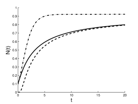
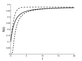
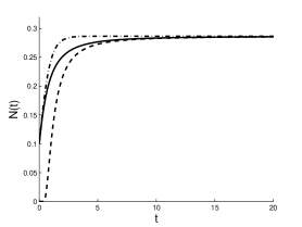
Figure 1: The proposed curve (full), Korf curve (dashed), and Gompertz curve (dot-dashed), for $y=0.1$, $\alpha=2$, $\beta=0.9,\,1.5,\,1.9$, respectively, with $C=0.93,\,0.38,\,0.29$.

Some interesting limit behaviors of the curves (8), (9) and (13) are shown in Table 1, for $\alpha\rightarrow 0$, $\alpha\rightarrow+\infty$, $\beta\rightarrow 0$ and $\beta\rightarrow+\infty$, with $t>0$. We observe that when the growth rate $\alpha$ goes to zero and when $\alpha$ goes to infinity, the three curves have all the same behavior, i.e. they tend to $y$ in the first case, and to $+\infty$ in the second case. Indeed, the population size exhibits a very pronounced growth when $\alpha$ is very large, since the carrying capacity tends to $+\infty$ when $\alpha$ diverges, due to (14). Moreover, for $\beta\rightarrow\infty$ the curves admit the same limit $y$, except for the Korf case when $0<t<1$.

In the following we analyze some features of the proposed model, and we perform some comparisons with the Gompertz and the Korf models.

Model $N_{\star}(t)$	$N_{\star}^{\prime}(0)$	$\displaystyle\lim_{\alpha\rightarrow 0}N_{\star}(t)$	$\displaystyle\lim_{\alpha\rightarrow\infty}N_{\star}(t)$	$\displaystyle\lim_{\beta\rightarrow 0}N_{\star}(t)$	$\displaystyle\lim_{\beta\rightarrow\infty}N_{\star}(t)$
Eq. (13)	$\alpha y$	$y$	$+\infty$	$y(1+t)^{\alpha}$	$y$
$y\exp{\left\{\frac{\alpha}{\beta}\left[1-(1+t)^{-\beta}\right]\right\}}$
Eq. (9)	$+\infty$	$y$	$+\infty$	$yt^{\alpha}$	$\left\{\begin{array}[]{ll}0,&0<t<1\\ y,&t\geq 1\end{array}\right.$
$y\exp{\left\{\frac{\alpha}{\beta}\left(1-t^{-\beta}\right)\right\}}$
Eq. (8)	$\alpha y$	$y$	$+\infty$	$ye^{\alpha t}$	$y$
$y\exp{\left\{\frac{\alpha}{\beta}\left(1-e^{-\beta t}\right)\right\}}$

Table 1: Some characteristics of models (8), (9) and (13).

2.1 The correction factor and the relative growth rate

Several growth models described by a function $N_{\star}(t)$ can be expressed in the form (see [29])

$$\frac{dN_{\star}(t)}{dt}=\beta N_{\star}(t)f\left[N_{\star}(t)\right].$$ (16)

The function $f$ is called a size covariate model since it is function of $t$ only through $N$ and it is widely used to represent the density dependent growth; indeed the relative growth rate $g$ (cf. [34]) is strictly related to $f$ via

$$g[N_{\star}(t)]:=\frac{1}{N_{\star}(t)}\frac{dN_{\star}(t)}{dt}\equiv\beta f[N_{\star}(t)].$$ (17)

Note that the function $f$ is also called correction factor because it expresses the deviation from the classical exponential growth (1), for which $f(z)=1$ for all $z\geq 0$.

A suitable choice of $f(z)$ is

$$f(z)=f_{N}(z):=\frac{\alpha}{\beta}\left(1-\frac{\beta}{\alpha}\log\frac{z}{y}\right)^{1+1/\beta},\qquad z>0,$$ (18)

which corresponds to the family of models given by

$$N_{\star}(t)=ye^{{\alpha}/{\beta}}\left[1-(t+D)^{-\beta}\right],\qquad t>0,$$

where $D$ is a constant. Note that if $D=1$ one obtains the model (13), whereas $D=0$ yields the Korf model (9). The Gompertz model is obtained by choosing

$$f(z)=f_{G}(z):=\frac{\alpha}{\beta}-\log\frac{z}{y},\qquad z>0,$$ (19)

this leading to the following family of population laws:

$$N(t)=ye^{{\alpha}/{\beta}}\exp{\left\{-e^{-\beta t}-D\right\}},\qquad t>0,$$

for $D=\alpha/\beta-1$. In Fig. 2 we compare the correction factor $f(z)$ for the models (8), (9) and (13), plotted against $\log z$. We note that the correction factor of the considered models are decreasing in $\beta$. Furthermore, from (18) and (19), for $C\equiv ye^{\alpha/\beta}$ we have

$$f_{N}(z)=1\quad\hbox{for }z=C\,e^{-\left(\frac{\alpha}{\beta}\right)^{1/(\beta+1)}}<C;\qquad f_{G}(z)\to 1\quad\hbox{for }z\to C.$$

Hence, for both the new model and the Korf model the correction factor is equal to that of the exponential growth for a given value of the population size $z$ (for $z$ smaller than the carrying capacity $C$). On the contrary, for the Gompertz model the correction factor tends to that of the exponential growth when $z$ tends to $C$.

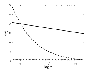
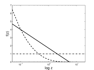
Figure 2: The correction factor for models (8) (solid line), (9) and (13) (dashed line), for $y=0.1$, $\alpha=2$, $\beta=0.1$ (left), $\beta=0.5$ (right), compared with $f(z)=1$ (dot-dashed line).

Regarding the relative growth rate $g$ given in (17), for models (9) and (13) we have $g^{\prime}(z)=-\frac{1+\beta}{z}\left(1-\frac{\beta}{\alpha}\log\frac{z}{y}\right)^{1/\beta}$, whereas, due to (19), for the Gompertz model (8) we have $g^{\prime}(z)=-\beta/z$. Since $0<z<ye^{\alpha/\beta}=C$, the relative growth rate $g(z)$ is decreasing for all the considered models, and reaches the minimum at the carrying capacity $C$.

2.2 The inflection point

Let us now focus on the inflection point of the growth model (13). Clearly, this is of high interest in population growth since for sigmoidal curves such point expresses the instant when the growth rate is maximum. From (12) we have

$$\frac{d^{2}N(t)}{dt^{2}}=\alpha(1+t)^{-(\beta+2)}N(t)\left[\alpha(1+t)^{-\beta}-\beta-1\right],\qquad t>0.$$

Hence, if $\alpha\leq\beta+1$ the curve (13) has downward concavity for all $t$, whereas if $\alpha>\beta+1$ then $N(t)$ is sigmoidal with inflection point

$$t_{N}=\left(\frac{\alpha}{\beta+1}\right)^{\frac{1}{\beta}}-1.$$ (20)

The population at the inflection point is given by

$$N(t_{N})=ye^{-1-\frac{1}{\beta}}e^{\frac{\alpha}{\beta}}=Ce^{-1-\frac{1}{\beta}},$$

where $C$ is the carrying capacity, given in (14).

In Table 2, the inflection points ($t_{N},\,t_{K},\,t_{G}$) and the population at the inflection points ($N(t_{N}),\,N_{K}(t_{K}),\,N_{G}(t_{G})$) are shown for the three models (13), (9) and (8), respectively. Note that

$$N_{K}(t_{K})=N(t_{N})<N_{G}(t_{G}).$$

Hence, whereas for a fixed time $t$ the considered growth curves are ordered according to (15), the latter equation shows that the new model and the Korf model evaluated at the inflection points have identical population size, which is smaller than that of the Gompertz model.

Let us now analyze some interesting limits of the population at the inflection point. From Table 2 we have, with $N_{K}(t_{K})=N(t_{N})$,

$$\lim_{\alpha\rightarrow 0}N(t_{N})=ye^{-1}e^{-\frac{1}{\beta}},\qquad\lim_{\beta\rightarrow+\infty}N(t_{N})=ye^{-1},$$

$$\lim_{\beta\rightarrow 0}N(t_{N})=\left\{\begin{array}[]{ll}+\infty,&\qquad\alpha>1\\ ye^{-1},&\qquad\alpha=1\\ 0,&\qquad\alpha<1,\end{array}\right.\qquad\lim_{\alpha\rightarrow+\infty}N(t_{N})=+\infty,$$

whereas for the Gompertz model it results

$$\lim_{\alpha\rightarrow 0}N_{G}(t_{G})=\lim_{\beta\rightarrow+\infty}N_{G}(t_{G})=ye^{-1},$$

$$\lim_{\beta\rightarrow 0}N_{G}(t_{G})=\lim_{\alpha\rightarrow+\infty}N_{G}(t_{G})=+\infty.$$

Model	Inflection	Population at the
	point	inflection point
Eq. (13)	$t_{N}=\left(\frac{\alpha}{\beta+1}\right)^{1/\beta}-1$, $\alpha>\beta+1$	$N(t_{N})=Ce^{-1-1/\beta}$
	$N$ is concave for $\alpha\leq\beta+1$
Eq. (9)	$t_{K}=\left(\frac{\alpha}{\beta+1}\right)^{1/\beta}$	$N_{K}(t_{K})=Ce^{-1-1/\beta}$
Eq. (8)	$t_{G}=\frac{1}{\beta}\log\left(\frac{\alpha}{\beta}\right)$, $\alpha>\beta$	$N_{G}(t_{G})=Ce^{-1}$
	$N_{G}$ is concave for $\alpha\leq\beta$

Table 2: The inflection points and the population sizes at the inflection points are shown for models (13), (9) and (8).

2.3 The maximum specific growth rate and the lag time

In several fields it is interesting to investigate a growth curve in proximity of the inflection point, by approximating linearly the curve in that point. This is typically of interest in phenomena that exhibit lag, growth, and asymptotic phases, such as the growing process of length or mass of some organisms or populations (see Zwietering et al. [38] for details). For a generic growth curve $N_{\star}(t)$ we introduce the maximum specific growth rate $\mu_{\star}$, defined as the coefficient of the tangent to the curve in the inflection point $t_{\star}$, i.e.

$$\mu_{\star}=\frac{dN_{\star}(t)}{dt}\Big{|}_{t=t_{\star}}.$$ (21)

Moreover, $\lambda_{\star}$ denotes the lag time defined as the $x$-axis intercept of this tangent. Specifically, sigmoidal functions describing evolutionary phenomena show a phase in which the specific growth rate starts at a zero value and then accelerates to a maximal value $\mu$ in a certain period of time, resulting in a lag time $\lambda$. The value of $\mu$ is given by the slope of the line when the grow is exponential.

For the model (13), for $\alpha>\beta+1$, recalling (12) and (20), due to (21) the maximum specific growth rate is

$$\mu_{N}=y\frac{(\beta+1)^{1/\beta+1}}{\alpha^{1/\beta}}\exp{\left\{\frac{\alpha-1}{\beta}-1\right\}}.$$ (22)

Moreover, recalling the expressions of $t_{N}$ and $N(t_{N})$ given in Table 2, the tangent curve in $\left(t_{N},\,N(t_{N})\right)$ is

$$n=\mu_{N}t+y\exp{\left\{\frac{\alpha-1}{\beta}-1\right\}}\left[\frac{(\beta+1)^{1/\beta+1}}{\alpha^{1/\beta}}-\beta\right],$$ (23)

with $\mu_{N}$ expressed in (22). (For notation clarity, we denote by $n$ the $y$-axis.) The lag time $\lambda_{N}$ for the model (13) is the $t$-axis intercept of (23), that is

$$\lambda_{N}=\beta\frac{\alpha^{1/\beta}}{(\beta+1)^{1/\beta+1}}-1;$$

note that $\lambda_{N}$ is positive if, and only if, $\alpha>(\beta+1)^{\beta+1}/\beta^{\beta}$.

$N_{\star}(t)$	$\mu_{\star}$	Intercept of	$\lambda_{\star}$
		tangent curve
$N(t)$	$y\frac{(\beta+1)^{\frac{1}{\beta}+1}}{\alpha^{\frac{1}{\beta}}}e^{\frac{\alpha-1}{\beta}-1}$	$ye^{\frac{\alpha-1}{\beta}-1}\left[\frac{(\beta+1)^{1/\beta+1}}{\alpha^{1/\beta}}-\beta\right]$	$\beta\frac{\alpha^{1/\beta}}{(\beta+1)^{1/\beta+1}}-1$
	($\alpha>\beta+1$)	($\alpha>\beta+1$)	$\left(\alpha>(\beta+1)^{\beta+1}/\beta^{\beta}\right)$
$N_{K}(t)$	$y\frac{(\beta+1)^{\frac{1}{\beta}+1}}{\alpha^{\frac{1}{\beta}}}e^{\frac{\alpha-1}{\beta}-1}$	$-y\beta e^{\frac{\alpha-1}{\beta}-1}$	$\lambda_{N}+1$
$N_{G}(t)$	$y\beta e^{\alpha/\beta-1}$	$ye^{\alpha/\beta-1}\left(1-\log\frac{\alpha}{\beta}\right)$	$\frac{1}{\beta}\log\frac{\alpha}{\beta}-\frac{1}{\beta}$
($\alpha>\beta$)

Table 3: The maximum specific growth rate, the intercept of tangent line and the lag time for the models (13), (9) and (8).

For comparison purposes, Table 3 shows the maximum specific growth rate, the intercept of the tangent curve and the lag time for the three models (8), (9) and (13). The tangent lines (dotted curves) and the lag times (asterisk points) for the three models are plotted in Fig. 3.

model (13)                                             model (9)

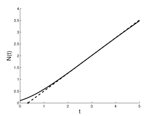
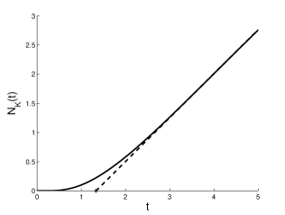
model (8)

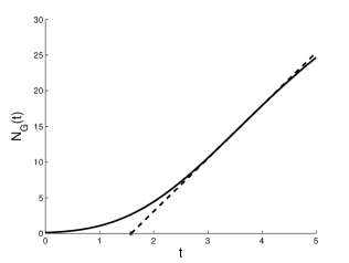
Figure 3: The tangent lines (dotted curves) and the lag times (asterisk points) with $y=0.1$, $\alpha=3$ and $\beta=0.5$.

2.4 Threshold crossing

Studies on population growth often focus on the time that the population size spends below (or above) a certain threshold, say $S$. For instance, the upward threshold crossing problem is relevant to determine suitable therapeutic protocols related to Gompertz-like growth model for tumor cells evolution (cf. [2]). Moreover, criteria based on threshold level crossing are also employed for intermittent cancer therapies (see [28]).

For an increasing growth model $N_{\star}(t)$, let us then analyze the time instant in which $N_{\star}(t)$ crosses $S$, with $S>N_{\star}(0)$. In the context of bounded populations, we consider as threshold a percentage $p$ of the carrying capacity $C$, so that

$$S=pC,\qquad N_{\star}(0)<S<C.$$

The (upward) threshold $S$ may represents a critical value in tumor cells dynamics or a superimposed boundary in population evolution. Taking into account the value of $C$ in (14) and that $N_{\star}(0)=y$, the following condition on $p$ holds for the model (13): $e^{-\alpha/\beta}<p<1$. Hence, denoting by $\theta_{N}$ the crossing time instant of $N(t)$ through the threshold $S$, and recalling (13) the solution of equation $N(\theta_{N})=pC$ is

$$\theta_{N}=\left(\frac{\beta}{\alpha}\log\frac{1}{p}\right)^{-\frac{1}{\beta}}-1,\qquad e^{-\alpha/\beta}<p<1.$$

Similarly, for the Korf and Gompertz models one has

$$\theta_{K}=\theta_{N}+1,\quad 0<p<1,\qquad\theta_{G}={-\frac{1}{\beta}}\log\left(\frac{\beta}{\alpha}\log\frac{1}{p}\right),\quad e^{-\alpha/\beta}<p<1,$$

respectively, with $\theta_{G}<\theta_{N}<\theta_{K}$. Such threshold crossing times are plotted in Fig. 4 as (increasing) function of $p$ in a suitable instance. As mentioned above, they could be employed for cancer therapies in order to establish suitable operational times in therapeutic protocols.

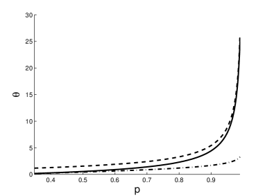
Figure 4: The threshold crossing times $\theta_{N}$ (full line), $\theta_{K}$ (dashed line) and $\theta_{G}$ (dot-dashed line) as function of $p$, with $0<p<1$ for the Korf model and $e^{-\alpha/\beta}<p<1$ for the others, with $\alpha=2$, $\beta=1.9$ and $y=0.1$.

3 Data analytic examples

In this section we consider some data analytic examples for which model (13) provides a good fit. We deal with the following data sets collected in Table 12.7 and Table 12.14 of Lindsey [18] in which a certain feature of the growth behavior of the small mammal pikas and of a colony of cells is recorded:

• the weight $n_{i}$ of a pregnant Afghan pikas (g) over $14$ equally spaced periods from conception to parturition, recorded during an experiment.

• the size $n_{i}$ of a closed colony of Paramecium aurelium are recorded at $18$ time instants in a given experiment.

A thorough description of the above data and the relevant experiments is provided in Lindsey [18]. The corresponding data are fitted by nonlinear regression thanks to the classical algorithm based on the minimization of the sum of the squares of the differences between the measured and predicted values. We use the routine lsqcurvefit of Matlab^®, that solves nonlinear curve-fitting (data-fitting) problems in least-squares sense, where the predicted values are obtained from the nonlinear equations of the models (8), (9) and (13). Once determined the parameters of the three models, in order to evaluate the attained approximations, we compare the growth curves by using the ISRP growth metric, introduced in Bhowmick et al. [6].

(i)                                                      (ii)

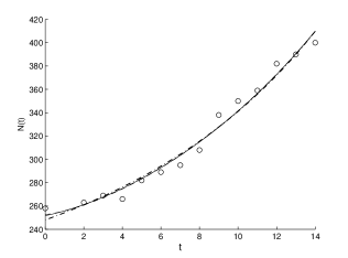
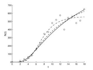
Figure 5: Interpolation of data sets (i), (ii) and (iii), under the growth models (13) (full), (9) (dashed) and (8) (dot-dashed).

For the three growth models, in Fig. 5 we show the interpolation of the data sets mentioned above. In both cases we have reasonably good fit of the data. We recall that the ISRP growth metric has been introduced recently in [6] aiming to determine the true growth curve that best fits the data (statistically). Indeed, such a metric provides an estimate of the rate parameter corresponding to the identified growth model in specific time intervals. Note that this is in contrast to the usual $R^{2}$-criterion, which does not allow to estimate the relevant parameters.

The differential equation (12) can be rewritten as

$$\frac{1}{N(t)}\frac{dN(t)}{dt}=\alpha(1+t)^{-(\beta+1)},\qquad t>0.$$

Hence, in an experimental framework in which the population is sampled through a suitable time interval, according to Bhowmick et al. [6] parameter $\alpha$ can be also interpreted as the “Overall Rate Parameter” (when it is computed for the entire experimental time frame) or as the “Interval Specific Rate Parameter” (ISRP), denoted by $\alpha(\Delta t)$ (when it is estimated on the basis of a specific time interval having width $\Delta t$). Consequently, under the initial condition $N(0)=y$, the growth law can be represented in the form

$$N(t)=ye^{\alpha s(t)},\qquad t\geq 0,$$ (24)

for a suitable function $s(t)$. Hence, the ISRP can be computed as

$$ISRP=\alpha(\Delta t)=\frac{1}{s(t+\Delta t)-s(t)}\log\left(\frac{N(t+\Delta t)}{N(t)}\right).$$ (25)

We note that for the Gompertz model, for the Korf model, and for the new proposed model, in all cases the growth curve has the form (24). Hence, due to Eqs. (8), (9) and (13), for the three models the function $s(t)$ is given, respectively, by

$$s_{G}(t)=\frac{1-e^{-\beta t}}{\beta},\quad s_{K}(t)=\frac{1-t^{-\beta}}{\beta},\quad s_{N}(t)=\frac{1-(1+t)^{-\beta}}{\beta}.$$

It follows that the ISRP for the three models is:

(i)                                                      (ii)

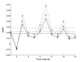
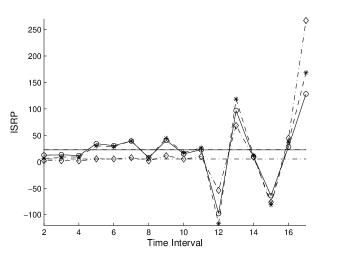
Figure 6: ISRP and the constant estimated rate $\alpha$ are plotted for the growth models (13) (full), (9) (dashed) and (8) (dot-dashed).

$$ISRP_{G}=\frac{\beta}{e^{-\beta t}-e^{-\beta(t+\Delta t)}}\log\left(\frac{N(t+\Delta t)}{N(t)}\right),$$

$$ISRP_{K}=\frac{\beta}{t^{-\beta}-(t+\Delta t)^{-\beta}}\log\left(\frac{N(t+\Delta t)}{N(t)}\right),$$

$$ISRP_{N}=\frac{\beta}{(1+t)^{-\beta}-(1+t+\Delta t)^{-\beta}}\log\left(\frac{N(t+\Delta t)}{N(t)}\right).$$

For a more tight comparison, the 3 models are then used to fit the datasets of cases (i) and (ii). Their comparative performances are discussed based on the ISRP metric. The extent of departure between the line of the constant rate parameter $\alpha$ of the corresponding growth law and the estimated ISRP reflects the deviation of the assumed model from the true law. The ISRP and the constant estimated rate $\alpha$ are plotted in Fig. 6 for the 3 models, in order to rank such models by means of the ISRP metric. We have the following estimated values of $\alpha$ in the two considered instances:

(i) $\alpha_{N}=0.0187$,  $\alpha_{K}=0.0222$,  $\alpha_{G}=0.0282$,

(ii) $\alpha_{N}=22.5261$,  $\alpha_{K}=23.0986$,  $\alpha_{G}=5.3504$.

Specifically, the proposed model (13) has the smallest average deviation of ISRP from the estimated parameter. Indeed, by computing the $d_{2}$-distance (in the euclidean norm) between ISRP and the constant parameter, for the given datasets, one has

(i) $d_{2}^{N}=0.0442$,  $d_{2}^{K}=0.0522$,  $d_{2}^{G}=0.0672$,

(ii) $d_{2}^{N}=200.2610$,  $d_{2}^{K}=250.3044$,  $d_{2}^{G}=290.2033$.

It thus follows that the smallest distance is obtained for the proposed model (13). Hence, the actual dynamics of the two datasets is better described by model (13) rather than the other two models.

4 Analysis of a special inhomogeneous linear birth-death process

Deterministic curves are often employed to describe population growth due to their ease of tractability. However they can be reasonably used just to describe overall dynamics. A more realistic description can be performed by means of stochastic models. Indeed, suitable random processes allow to take into account the ubiquitous environmental fluctuations, which are due to various factors that are unknown or not always quantifiable. As example, we recall the paper by Tan [30], that investigates a birth-death process whose mean is identical to the curve of the Gompertz growth. A general theory based on stochastic differential equations is proposed by Tan et al. [31] to construct models for carcinogenesis and to analyze related data. A non-homogeneous density-dependent birth-death process describing a stochastic logistic growth has been investigated by Tan and Piantadosi [32]. More recently, aiming to describe the effect of radiation therapy, Tuckwell [35] considered the differential equation of Gompertzian growth modified by inclusion of a stochastic term involving the Poisson process.

In order to propose a stochastic counterpart of the growth model introduced in (13), in this section we shall investigate an evolutionary model based on a birth-death process. Since a population described by the curve (13) can reach a great size when $\alpha$ is large, we are driven to consider a stochastic process having infinite state-space. Specifically, we assume that the number of individuals of a population is described by an inhomogeneous linear birth-death process $\left\{X(t);\,t\geq 0\right\}$ having state space $\mathbb{N}_{0}$, with 0 absorbing endpoint. The birth and death rates are specified by

$$\begin{array}[]{ll}P[X(t+h)=j+1\,|\,X(t)=j]=j\lambda(t)h+o(h),&\qquad j\in\mathbb{N}_{0}\\[2.84526pt] P[X(t+h)=j-1\,|\,X(t)=j]=j\mu(t)h+o(h),&\qquad j\in\mathbb{N},\end{array}$$ (26)

where $\lambda(t)$ and $\mu(t)$ are positive functions, integrable on $(0,t)$ for any finite $t>0$, and $h>0$. Since the rates (26) are linear in $j$, new births and deaths occur proportionally to the population size, and according to the time-dependent rates $\lambda(t)$ and $\mu(t)$, which constitute the individual birth rate and death rate at time $t$, respectively. We recall that the model specified in (26) is a time-inhomogeneous version of the classical linear birth-death process (see, for instance, Bailey [3]); examples of applications of such a model in genetics and phylogenetics have been reviewed in Novozhilov et al. [20].

For all $t\geq 0$, and $x,y\in\mathbb{N}_{0}$ we denote the transition probability of $X(t)$ by $P_{y,x}(t)=P[X(t)=x\,|\,X(0)=y]$. Clearly, $P_{y,x}(t)$ represents the probability that the population size equals level $x$ at time $t$, conditional on the initial size $y$. Formally, the initial state $y$ may be 0, however this choice is trivial since 0 is an absorbing endpoint for the birth-death process. Henceforth we thus assume $X(0)=y\in\mathbb{N}$, in agreement with the fact that the initial state of the growth model (13) is positive.

Aiming to determine the transition probability, for $0<z<1$ and $t\geq 0$, let $G(z,t)=\sum_{x=0}^{\infty}P_{y,x}(t)z^{x}$ be the probability generating function of $X(t)$, with initial condition $G(z,0)=z^{y}$. As showed in Tan [30], it results

$$G(z,t)=\left\{1-(z-1)[(z-1)\phi(t)-\psi(t)]^{-1}\right\}^{y},$$ (27)

where

$$\psi(t)=\exp{\left\{-\int_{0}^{t}[\lambda(\tau)-\mu(\tau)]d\tau\right\}},\qquad\phi(t)=\int_{0}^{t}\lambda(\tau)\psi(\tau)d\tau.$$ (28)

For brevity, in the following we denote the conditional mean and the conditional variance of $X(t)$, given $X(0)=y$, by

$$E_{y}(t)=E[X(t)|X(0)=y]\quad\hbox{and}\quad V_{y}(t)=Var[X(t)|X(0)=y],$$

respectively. Clearly, $E_{y}(t)$ and $V_{y}(t)$ describe the mean trend and the related variability in the stochastic growth model. From assumptions (26) we obtain that the population mean satisfies the following differential equation:

$$\frac{dE_{y}(t)}{dt}=\xi(t)E_{y}(t),\qquad t>0,$$ (29)

where the time-dependent growth rate $\xi(t)$ is the net growth rate per capita of individuals, i.e.

$$\xi(t)=\lambda(t)-\mu(t),\qquad t\geq 0.$$ (30)

The behavior of $X(t)$ may mimic the growth curve proposed in (13). Indeed, the analogies between the growth model (13) and the considered birth-death process stems from the fact that Eq. (29) has the same form of (10). Hence, the growth model (13) and the mean of the birth-death process $X(t)$ are governed by the same equation in the special case when the assumptions (11) and (30) hold. This case will be treated in Section 4.1.

Let us now obtain the transition probabilities, the conditional mean and the conditional variance of $X(t)$.

Proposition 1

Let $y\in\mathbb{N}$. The transition probabilities of the process $X(t)$, with rates (26), are given by:

$$P_{y,0}(t)=\left(1-\frac{1}{\psi+\phi}\right)^{y},$$ (31)

$$P_{y,x}(t)=\left(\frac{\phi}{\psi+\phi}\right)^{x}\,\sum_{i=0}^{m}{y\choose u}{y+x-i-1\choose y-1}(\phi^{-1}-1)^{i}\left(1-\frac{1}{\psi+\phi}\right)^{y-i}$$

$$\hskip 284.52756ptx\in\mathbb{N},$$

with $m=\min\left\{y,x\right\}$, where $\psi=\psi(t)$ and $\phi=\phi(t)$ are shown in (28). Moreover, the conditional mean and the conditional variance of $X(t)$ are

$$E_{y}(t)=\frac{y}{\psi(t)},\qquad V_{y}(t)=y\,\frac{[\psi(t)+2\phi(t)-1]}{\psi^{2}(t)},\qquad t\geq 0,$$ (32)

respectively.

• The probability generating function given in (27) can be rewritten as the product of two generating functions, i.e.

  $$G(z,t)=\left({1-z\;\frac{\phi}{\phi+\psi}}\right)^{-y}\left({z\;\frac{1-\phi}{\phi+\psi}+1-\frac{1}{\phi+\psi}}\right)^{y}.$$

  Since $0<\frac{\phi}{\phi+\psi}<1$, for $0<z<1$ one has

  $$\left(1-z\;\frac{\phi}{\phi+\psi}\right)^{-y}=\sum_{i=0}^{\infty}a_{i}z^{i},\qquad\left(z\;\frac{1-\phi}{\phi+\psi}+1-\frac{1}{\phi+\psi}\right)^{y}=\sum_{i=0}^{\infty}b_{i}z^{i},$$

  where

  $$a_{i}={y+i-1\choose y-1}\left(\frac{\phi}{\phi+\psi}\right)^{i},\qquad i\in\mathbb{N}_{0}$$

  and

  $$b_{i}={y\choose i}\left(\frac{1-\phi}{\phi+\psi}\right)^{i}\left(1-\frac{1}{\phi+\psi}\right)^{y-i}{\bf 1}_{\{0\leq i\leq y\}}.$$

  Therefore, we have $P_{y,x}(t)=\sum_{i=0}^{x}b_{i}a_{x-i}$ and the expressions (31) thus follow. Finally, the conditional mean and the conditional variance (32) can be obtained from (27) straightforwardly.

It is worth pointing out that the expressions (31) actually correct the transition probabilities given in Tan [30].

The monotonicity and the concavity of the conditional mean and variance of $X(t)$ can be analyzed in term of $\lambda(t)$ and $\mu(t)$ by noting that, due to (32), for $t\geq 0$ we have

$$E_{y}^{\prime}(t)=y\frac{\xi(t)}{\psi(t)},\qquad E_{y}^{\prime\prime}(t)=y\frac{\lambda^{\prime}(t)-\mu^{\prime}(t)+\xi^{2}(t)}{\psi(t)},$$

$$V_{y}^{\prime}(t)=\frac{y}{\psi^{2}(t)}\left\{\lambda(t)[3\psi(t)+4\phi(t)-2]-\mu(t)[\psi(t)+4\phi(t)-2]\right\},$$

$$V^{\prime\prime}_{y}(t) = \frac{y}{\psi^{2}(t)}\left\{\lambda^{\prime}(t)\left[3\psi(t)+4\phi(t)-2\right]-\mu^{\prime}(t)\left[\psi(t)+4\phi(t)-2\right]\right.$$

$$+\lambda(t)\left[\xi(t)(3\psi(t)+8\phi(t)-4)+4\lambda(t)\psi(t)\right]$$

$$\left.-\mu(t)\left[\xi(t)(\psi(t)+8\phi(t)-4)+4\lambda(t)\psi(t)\right]\right\},$$

where $\xi(t)$ is the net growth rate defined in (30). It immediately follows that the population mean is increasing (decreasing) at time $t$ if $\xi(t)$ is positive (negative). The concavity of the mean and the monotonicity and concavity of the variance can be studied through suitable computations. From the above expressions, some results on the conditional mean and variance are provided in Table 4, where ${\cal D}$ means that the result strictly depends on the rates $\lambda(t)$ and $\mu(t)$, and where we have set

$$\tilde{\psi}=\lim_{t\rightarrow\infty}\psi(t),\quad\tilde{\phi}=\lim_{t\rightarrow\infty}\phi(t),\quad\tilde{\lambda}=\lim_{t\rightarrow\infty}\int_{0}^{t}\lambda(\tau)d\tau,\quad\tilde{\mu}=\lim_{t\rightarrow\infty}\int_{0}^{t}\mu(\tau)d\tau.$$ (33)

It is shown that the present model can exhibit very different behaviors, according to the values of the relevant parameters. For instance, the conditional mean may increase toward $\infty$ and decrease to a constant (possibly vanishing) asymptotic value.

$\!\!\!\!\xi(t)$	$E_{y}(t)$	$\displaystyle\lim_{t\rightarrow\infty}E_{y}(t)$	$V_{y}(t)$	$\displaystyle\lim_{t\rightarrow\infty}V_{y}(t)$
$\!\!\!\!>0\;\;\forall t>0$	$\begin{array}[]{l}\hbox{strictly}\\ \hbox{increas.}\end{array}$	$\left\{\begin{array}[]{ll}y/\tilde{\psi},&\hbox{if }\tilde{\lambda}-\tilde{\mu}<\infty\\ \infty,&\hbox{if }\tilde{\lambda}-\tilde{\mu}=\infty\end{array}\right.$	$\begin{array}[]{l}\hbox{strictly}\\ \hbox{increas.}\end{array}$	$\left\{\begin{array}[]{l}y(\tilde{\psi}+2\tilde{\phi}-1)/\tilde{\psi}^{2},\\ \qquad\quad\hbox{if }\tilde{\lambda}<\infty,\tilde{\mu}<\infty\\ \infty,\qquad\hbox{if }\tilde{\lambda}=\infty\end{array}\right.$
$\!\!\!\!=0\;\;\forall t>0$	constant	$y$	$\begin{array}[]{l}\hbox{strictly}\\ \hbox{increas.}\end{array}$	$\left\{\begin{array}[]{ll}2y\tilde{\lambda},&\hbox{if }\tilde{\lambda}<\infty\\ \infty,&\hbox{if }\tilde{\lambda}=\infty\end{array}\right.$
$\!\!\!\!<0\;\;\forall t>0$	$\begin{array}[]{l}\hbox{strictly}\\ \hbox{decreas.}\end{array}$	$\left\{\begin{array}[]{ll}y/\tilde{\psi},&\hbox{if }\tilde{\mu}-\tilde{\lambda}<\infty\\ 0,&\hbox{if }\tilde{\mu}-\tilde{\lambda}=\infty\\ \end{array}\right.$	${\cal D}$	$\left\{\begin{array}[]{l}y(\tilde{\psi}+2\tilde{\phi}-1)/\tilde{\psi}^{2},\\ \qquad\quad\hbox{if }\tilde{\lambda}<\infty,\tilde{\mu}<\infty\\ {\cal D},\qquad\hbox{otherwise}\end{array}\right.$

Table 4: Some results on the conditional mean and variance of $X(t)$.

We finally remark that, since 0 is an absorbing endpoint, $P_{y,0}(t)$ represents the probability that the population reaches extinction prior to time $t$. Due to (31), the probability of ultimate extinction, for initial state $y$, is given by

$$\pi_{y,0}:=\lim_{t\to\infty}P_{y,0}(t)=\left(1-\frac{1}{\tilde{\psi}+\tilde{\phi}}\right)^{y},\qquad y\in\mathbb{N}.$$ (34)

Clearly, if $\tilde{\mu}-\tilde{\lambda}=\infty$ or $\tilde{\phi}=\infty$, then $\pi_{y,0}=1$, this leading to certain ultimate extinction.

4.1 Analysis of a special case

We already pointed out that the growth model (13) and the conditional mean of the birth-death process $X(t)$ satisfy the same linear differential equation, when both Eqs. (11) and (30) hold. The aim of this section is to investigate in detail such a special case.

Proposition 2

The linear birth-death process with rates specified in (26) has conditional mean

$$E_{y}(t)=y\exp{\left\{\frac{\alpha}{\beta}\left[1-(1+t)^{-\beta}\right]\right\}},\qquad t\geq 0$$ (35)

if and only if

$$\lambda(t)-\mu(t)=\alpha(1+t)^{-(\beta+1)},\qquad t\geq 0.$$ (36)

• From the first of (28) and (32) we have

  $$E_{y}(t)=y\exp{\left\{\int_{0}^{t}[\lambda(\tau)-\mu(\tau)]d\tau\right\}},\qquad t\geq 0.$$

  Hence, the expression (35) holds if and only if

  $$\int_{0}^{t}[\lambda(\tau)-\mu(\tau)]d\tau=\frac{\alpha}{\beta}\left[1-(1+t)^{-\beta}\right],\qquad t\geq 0,$$ (37)

  that is equivalent to (36).

Let us now investigate the process $X(t)$ under the assumption (36). In this case, the birth rate is larger than the death rate, and the net growth rate defined in (30) is decreasing and tends to zero according to a power law. Hence, this assumption leads to results useful to describe populations that experience a tendential high growth for initial time, which however decreases in time. Furthermore, by virtue of (28), the mean $E_{y}(t)$ is identical to the curve $N(t)$ given in (13). Hence, due to (36), from (37) one has $\tilde{\lambda}-\tilde{\mu}={\alpha}/{\beta}$, with $\tilde{\lambda}$ and $\tilde{\mu}$ defined in (33). From the results shown in Table 4, $E_{y}(t)$ is strictly increasing, and clearly it tends to the carrying capacity, i.e. $\displaystyle\lim_{t\to\infty}E_{y}(t)=ye^{\alpha/\beta}\equiv C$. Moreover, the function $\psi(t)$ is given by

$$\psi(t)=\exp{\left\{-\frac{\alpha}{\beta}\left[1-\left(1+t\right)^{-\beta}\right]\right\}},\qquad t\geq 0,$$ (38)

with $\tilde{\psi}=e^{-\alpha/\beta}$, so that the variance $V_{y}(t)$ is strictly increasing in $t$, according to the results specified in Table 4.

Example 1

Let Eq. (36) be satisfied. We now consider various instances of $\mu(t)$ listed in Table 5. The corresponding transition probabilities $P_{y,x}(t)$, given in (31), are plotted in Fig. 7 for $y=1$, $x=0$ and $x=1$, and for some choices of the parameters. The asymptotic absorption probability (34) is provided in the last column of Table 5. Note that in the first three cases of Table 5 we have $\tilde{\mu}=+\infty$, and thus $\tilde{\psi}=+\infty$, this implying that $\pi_{y,0}=1$, i.e. the ultimate extinction is certain when the individual death rate $\mu(t)$ is constant, or is a ramp function, or is sinusoidal. On the contrary, in case (d) it is $\tilde{\mu}<+\infty$, and thus $\tilde{\psi}<+\infty$, so that $\pi_{y,0}<1$. Specifically, if the individual birth and death rates are proportional and follow a decreasing power-law rule, then the ultimate extinction is not certain and is decreasing in $y$ (the initial population size).

case	$\mu(t)$	$\pi_{y,0}$
(a)	$A$	$1$
(b)	$A+B\,(t-t_{0}){\bf 1}_{\{t\geq t_{0}\}}$	$1$
(c)	$A+B\,\sin\left(\frac{2\pi}{Q}t\right)$	$1$
(d)	$A\,(1+t)^{-(\beta+1)}$	$\left[\frac{\frac{A}{\alpha}\left(1-e^{-\frac{\alpha}{\beta}}\right)}{\frac{A}{\alpha}\left(1-e^{-\frac{\alpha}{\beta}}\right)+1}\right]^{y}$

Table 5: Some choices of $\mu(t)$ and the corresponding extinction probabilities (34). Parameters $A$, $B$, $Q$ and $t_{0}$ are positive constants.

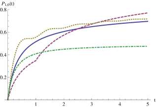
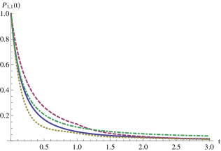
Figure 7: Probabilities $P_{1,0}(t)$ and $P_{1,1}(t)$ for the cases specified in Table 5, with (a) $A=2.00001$ (full line), (b) $B=1$, $A=2.00001$, $t_{0}=1$ (dashed line), (c) $A=2.00001$, $B=2$, $Q=1$ (dotted line), (d) $A=2.00001$ (dot-dashed line).

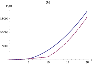
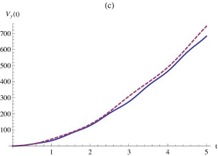
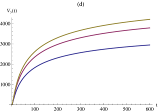
Figure 8: For $y=1,\,\alpha=2,\,\beta=0.5$, the variance $V_{y}(t)$ is plotted for the cases of Table 5. In case (a): $A=0.4,\,0.8,\,1$ (from bottom to top). In case (b): $A=1$, $B=1$, $t_{0}=5$ (solid line) and $t_{0}=10$ (dashed line). In case (c): $A=2.00001$, $B=2$, $Q=1$ (solid line) and $Q=2$ (dashed line). In case (d): $A=0.4,\,0.8,\,1$ (from bottom to top), where the limits of $V_{y}(t)$ as $t\to\infty$ are $4096.9,5267.45,5852.72$, respectively.

We now study the variance $V_{y}(t)$ when Eq. (36) holds, for the choices of $\mu(t)$ given in Table 5, with $\psi(t)$ specified in (38).

• Let us assume that $\mu(t)=A$, with $A>0$. This case refers to populations that experience constant individual death rate, regardless of age. Due to (32) the variance is

  $$V_{y}(t)=\frac{y}{\psi^{2}(t)}\left\{1-\psi(t)-\frac{2A}{\beta}\left(-\frac{\alpha}{\beta}\right)^{\frac{1}{\beta}}e^{-\frac{\alpha}{\beta}}\gamma\right\},\qquad t\geq 0,$$

  with $\gamma=\Gamma\left(-\frac{1}{\beta},-\frac{\alpha}{\beta}\right)-\Gamma\left(-\frac{1}{\beta},-\frac{\alpha}{\beta}(1+t)^{-\beta}\right)$, where $\Gamma(\cdot,\cdot)$ is the upper incomplete Gamma function.

• We consider $\mu(t)=A+B\,(t-t_{0}){\bf 1}_{\{t\geq t_{0}\}}$, with $A>0$, $B>0$ and $t_{0}>0$. In this case the individual death rate is constant until time $t_{0}$ and is linear increasing afterward, for instance due to worsening of the environmental or individual conditions. The variance has a rather cumbersome form, and thus it is omitted for brevity.

• Let $\mu(t)=A+B\sin\left(\frac{2\pi}{Q}t\right)$, where $Q>0$ and $A>|B|>0$. In this case the individual death rate is sinusoidal, thus describing populations that are subject to periodic increase and decrease of mortality, for instance due to seasonal predation or environmental variability. The variance can be expressed in integral form. Again, we omit the result for brevity.

• Let $\mu(t)=A(1+t)^{-(\beta+1)}$, with $A>0$, so that the individual birth and death rates are proportional and follow a decreasing power-law rule; from (32) one obtains the variance

  $$V_{y}(t)=\frac{y\left(1+2\frac{A}{\alpha}\right)\left(1-e^{-\frac{\alpha}{\beta}[1-(1+t)^{-\beta}]}\right)}{e^{-\frac{2\alpha}{\beta}[1-(1+t)^{-\beta}]}},\qquad t\geq 0.$$

Note that in the first three cases the variance diverges as $t\to\infty$, whereas in case (d) it tends to a constant. Some plots of $V_{y}(t)$ are shown in Fig. 8, showing that the shape of the variance depends on $\mu(t)$.

We point out that even though the birth-death process considered in this section has conditional mean identical to the growth curve (13), the behavior of the sample paths of $X(t)$ may be significantly different from such growth curve, since they can be absorbed at zero (recall Eqs. (31) and (34)). Although this characteristic allows $X(t)$ to be more realistic for some biological applications, in order to make the stochastic process closer to the growth curve, hereafter we remove the possibility of downward jumps. This leads to a birth process, that is clearly more appropriate to describe pure growth phenomena since its sample paths are non-decreasing.

5 Analysis of a special time-inhomogeneous linear birth process

In this section we investigate a time-inhomogeneous birth process, which is a special case of the process studied in Section 4.1, whose mean is identical to the growth curve proposed in Eq. (13).

Assume that $\mu(t)\equiv 0$ in Eq. (26), so that the number of individuals of a population is now modeled by an inhomogeneous linear birth process $\left\{X(t);\,t\geq 0\right\}$. Let ${\cal S}=\{y,y+1,\ldots\}$ be the state space of $X(t)$, where $y\in\mathbb{N}$ is the initial state, and let

$$P[X(t+h)=j+1|X(t)=j]=j\lambda(t)h+o(h),\qquad j\in{\cal S}$$ (39)

$$P[X(t+h)=j|X(t)=j]=1-j\lambda(t)h+o(h),\qquad j\in{\cal S},$$

where $\lambda(t)$ is a continuous positive function, integrable on $(0,t)$ for any finite $t>0$. Again, let $P_{y,x}(t)=P[X(t)=x\,|\,X(0)=y]$ be the transition probabilities of $X(t)$. It is well known (see [24], for instance) that for $y\in\mathbb{N}$ and $x\in{\cal S}$ we have

$$P_{y,x}(t)={x-1\choose y-1}e^{-y\Lambda(t)}\left(1-e^{-\Lambda(t)}\right)^{x-y},\qquad t\geq 0,$$ (40)

where

$$\Lambda(t)=\int_{0}^{t}\lambda(s)ds,\qquad t\geq 0.$$ (41)

In agreement with Proposition 2, the following result holds.

Proposition 3

The linear birth process with rates specified in (39) has conditional mean (35) if and only if

$$\lambda(t)=\alpha(1+t)^{-(\beta+1)},\qquad t\geq 0.$$ (42)

Hence, when the expression of $\lambda(t)$ is specified as in (42), we have $\Lambda(t)={\frac{\alpha}{\beta}\left[1-(1+t)^{-\beta}\right]}$, so that $\int_{0}^{\infty}\lambda(x)dx=\frac{\alpha}{\beta}$. Such model thus describes births under limited resources, with inputs that decrease in time and lead to a saturation level for the process. Indeed, according to [24], in this case both the conditional mean and variance are strictly increasing, with finite limits

$$E_{y}(t)=ye^{\frac{\alpha}{\beta}\left[1-(1+t)^{-\beta}\right]}\quad\stackrel{{\scriptstyle t\rightarrow+\infty}}{{\rightarrow}}\quad ye^{\frac{\alpha}{\beta}}\equiv C,$$ (43)

$$V_{y}(t)=ye^{\frac{\alpha}{\beta}\left[1-(1+t)^{-\beta}\right]}\left(e^{\frac{\alpha}{\beta}\left[1-(1+t)^{-\beta}\right]}-1\right)\quad\stackrel{{\scriptstyle t\rightarrow+\infty}}{{\rightarrow}}\quad ye^{\frac{\alpha}{\beta}}\left(e^{\frac{\alpha}{\beta}}-1\right).$$ (44)

Note that both $E_{y}(t)$ and $V_{y}(t)$ are decreasing in $\beta>0$. This is confirmed by Fig. 9, where the mean and variance of $X(t)$ are plotted for various choices of $\beta$. For this special model, differently from the previous cases, we can determine a closed form for the index of dispersion, also known as Fano factor, defined as the variance over mean. Indeed, from Eqs.  (43) and (44) we have

$$D_{y}(t):=\frac{V_{y}(t)}{E_{y}(t)}=e^{\frac{\alpha}{\beta}\left[1-(1+t)^{-\beta}\right]}-1\quad\stackrel{{\scriptstyle t\rightarrow+\infty}}{{\rightarrow}}\quad e^{\frac{\alpha}{\beta}}-1,$$ (45)

so that the index of dispersion is monotonic increasing in $t$, with $D_{y}(0)=0$. From (45) we have the following:
(i)  If $\alpha<\beta\log 2$ then the birth process $X(t)$ is underdispersed, i.e. $D_{y}(t)<1$ for all $t\geq 0$. In this case the occurrence of events (births) is more regular than that of a Poisson process.
(ii)  If $\alpha>\beta\log 2$ then $X(t)$ is underdispersed for $t<t_{*}$, with $t_{*}:=\left(1-\frac{\beta}{\alpha}\ln 2\right)^{-1/\beta}-1$, and $X(t)$ is overdispersed for $t>t_{*}$, i.e. for large times there is more irregularity in the distribution of the number of occurrence of events (births) with respect to a Poisson process.

Moreover, from (43) and (44) we have that the coefficient of variation of $X(t)$ is given by

$$\sigma_{y}(t)=\frac{\sqrt{V_{y}(t)}}{E_{y}(t)}=y^{-1/2}\sqrt{1-e^{-\frac{\alpha}{\beta}\left[1-(1+t)^{-\beta}\right]}},\qquad t\geq 0.$$

Hence, it follows that $\sigma_{y}(t)$ is increasing in $t$ and in $\alpha$, whereas it is decreasing in $\beta$. The following limits thus hold:

$$\sigma_{y}(t)\quad\stackrel{{\scriptstyle t\rightarrow+\infty}}{{\rightarrow}}\quad y^{-1/2}\sqrt{1-e^{-\frac{\alpha}{\beta}}},$$

$$\lim_{\alpha\rightarrow 0}\sigma_{y}(t)=0,\qquad\lim_{\alpha\rightarrow+\infty}\sigma_{y}(t)=y^{-1/2},$$

$$\lim_{\beta\rightarrow 0}\sigma_{y}(t)=y^{-1/2}\sqrt{1-(1+t)^{-\alpha}},\qquad\lim_{\beta\rightarrow+\infty}\sigma_{y}(t)=0.$$

Consequently, a better agreement between the deterministic growth model (13) and the birth process with rates (39) is attained when $\alpha\rightarrow 0$ or $\beta\rightarrow+\infty$. Note that such conditions both imply $\lambda(t)\to 0$, so that a good correspondence between the two models is expected for a low birth rate.

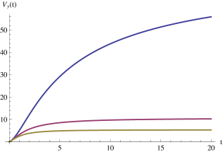
Figure 9: The mean (43) and the variance (44) are plotted for $y=1$, $\alpha=2$, $\beta=0.9,\,1.5,\,1.9$ (from top to bottom). The limits (carrying capacity) for the mean are $C=9.23,\,3.79,\,2.87$, whereas for the variance the limits are $75.92,\,10.60,\,5.34$, respectively.

Let us now discuss a first-passage-time problem for $X(t)$, in analogy with the threshold crossing problem analyzed in Section 2.4. The determination and analysis of first-passage-time densities in biological modeling deserve large interest, since such functions provide essential information on the probability that some critical or beneficial levels are attained by the stochastic process under investigation. Given the initial state $y\in{\cal S}$ and a fixed threshold $k\in\mathbb{N}$, with $k>y$, we consider the first-passage time

$$T_{y,k}=\inf\{t\geq 0:\,X(t)=k\},\qquad X(0)=y,$$

and denote by $g_{y,k}(t)=dP(T_{y,k}\leq t)/dt$ its probability density function (pdf). Since the sample-paths of $X(t)$ are increasing over the state space $\cal S$, it is not hard to see that, for $k\in\mathbb{N}$, $k>y$, we have

$$g_{y,k}(t)=(k-1)\lambda(t)P_{y,k-1}(t),\qquad t\geq 0,$$ (46)

where $\lambda(t)$ and $P_{y,k}(t)$ are given in (42) and (40), respectively. Note that, since $\lambda(0)=\alpha$, the initial value of the first-passage-time pdf is

$$\lim_{t\rightarrow 0}g_{y,k}(t)=\left\{\begin{array}[]{ll}\alpha\,y,&\quad\hbox{if }k=y+1\\ 0,&\quad\hbox{otherwise}.\end{array}\right.$$

In Fig. 10 the pdf of $T_{y,k}$ is plotted for various choices of $k$. We remark that such density is unimodal.

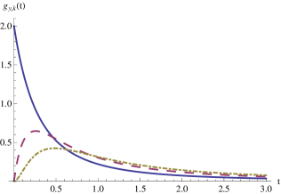
Figure 10: Density (46) for $\alpha=2,\,\beta=0.5$; on the left: $k=2,\,3,\,4$ (solid, dashed, dot-dashed line) and $y=1$; on the right: $k=3,\,4,\,5$ (solid, dashed, dot-dashed line) and $y=2$.

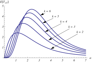
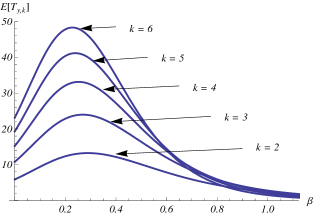
Figure 11: For $y=1$, the mean of $T_{y,k}$ is plotted as function of $\alpha$ with $\beta=1$ on the left, and as function of $\beta$ with $\alpha=1$ on the right.

In Fig. 11 the mean of $T_{y,k}$ is plotted as function of $\alpha$ and $\beta$, for various choices of $k$, evaluated by means of numerical integration. In both cases $E[T_{y,k}]$ is not monotonic, but it is increasing (decreasing) for small (large) values of $\alpha$ and $\beta$.

Concluding remarks

This paper has been devoted to the analysis of a deterministic growth model which is bounded by a carrying capacity, and behaves like the Gompertz law for small times, and the Korf law for large times. We investigated various properties of such a model, with attention to the main characteristics of interest in growth models, and performed various comparisons. Some examples of application of the proposed curve for the description of real growth phenomena have been shown, supported by an analysis of the performance based on suitable parameters.

In order to study a stochastic counterpart of the proposed model, we investigated a linear time-inhomogeneous birth-death process whose mean is identical to the proposed deterministic model. We obtained the transition probabilities, the moments and the population extinction of this process. However, even if the mean of such stochastic process is identical to the proposed growth curve, the considered birth-death model possesses an absorbing endpoint at zero and thus it may be not appropriate to describe a growth behavior. Hence, in order to overcome this drawback we finally studied a time-inhomogeneous birth process, whose mean again corresponds to the proposed growth curve, thus being more suitable to describe a pure growth phenomenon. The choices of the involved parameters that yield a better agreement between the deterministic growth model and the birth process have been identified though the analysis of the index of dispersion and the coefficient of variation.

Acknowledgements

This research was partially supported by the group GNCS of INdAM. The authors warmly thank the anonymous referees for various helpful comments.

References

- [1] H. Aagaard-Hansen, G.F. Yeo, A stochastic discrete generation birth, continuous death population growth model and its approximate solution, J. Math. Biol. 20 (1984) 69–90.
- [2] G. Albano, V. Giorno, A stochastic model in tumor growth, J. Theor. Biol. 242 (2006) 229–236.
- [3] N.T.J. Bailey, The elements of stochastic processes with applications to the natural sciences. Reprint of the 1964 original. Wiley, New York, 1990.
- [4] D.R. Berger, Comparison of the Gompertz and logistic equations to describe plant disease progress, Phytopathology 71 (1980) 716–719.
- [5] A.R. Bhowmick, S. Bhattacharya, A new growth curve model for biological growth: Some inferential studies on the growth of Cirrhinus mrigala, Math. Biosci. 254 (2014) 28–41.
- [6] A.R. Bhowmick, G. Chattopadhyay, S. Bhattacharya, Simultaneous identification of growth law and estimation of its rate parameter for biological growth data: a new approach, J. Biol: Phys. 40 (2014) 71–95.
- [7] J.H. Cha, M. Finkelstein, Justifying the Gompertz curve of mortality via the generalized Polya process of shocks, Theor. Popul. Biol. 109 (2016) 54–62.
- [8] F.W. Crawford, M.A. Suchard, Transition probabilities for general birth-death processes with applications in ecology, genetics, and evolution, J. Math. Biol. 65 (2012) 553–580.
- [9] A. Di Crescenzo, V. Giorno, A.G. Nobile, Constructing transient birth–death processes by means of suitable transformations, Appl. Math. Comput. 281 (2016) 152–171.
- [10] B. Gompertz, On the nature of the function expressive of the law of human mortality, and on a new mode of determining the value of life contingencies, Philos. Trans. R. Soc. Lond. 155 (1825) 513–583.
- [11] R. Gutierrez-Jaimez, P. Román, D. Romero, J.J. Serrano, F. Torres, A new Gompertz-type diffusion process with application to random growth, Math. Biosci. 208 (2007) 147–165.
- [12] T. Islam, D.G. Fiebig, N. Meade, Modelling multinational telecommunications demand with limited data, Intern. J. Forecast. 18 (2002) 605–624.
- [13] G.P. Karev, Non-linearity and heterogeneity in modelling of population dynamics, Math. Biosci. 258 (2014) 85–92.
- [14] V. Korf, Prìspevek k matematickè formulaci vzrustovèho zàkona lesnìch porostu [Contribution to mathematical definition of the law of stand volume growth], Lesnickà pràce 18 (1939) 339–379.
- [15] P.R. Koya, A.T. Goshu, Generalized mathematical model for biological growths, Open. J. Model. Simulation 1 (2013) 42–53.
- [16] A.K. Laird, Dynamics of tumor growth, Br. J. Cancer 18 (1964) 490–502.
- [17] A.K. Laird, Dynamics of tumor growth: comparison of growth rates and extrapolation of growth curve to one cell, Br. J. Cancer 19 (1965) 278–291.
- [18] J.K. Lindsey, Statistical Analysis of Stochastic Processes in Time, Cambrige University Press, New York, 2004.
- [19] E. Milotti, V. Vyshemirsky, M. Sega, R. Chignola, Interplay between distribution of live cells and growth dynamics of solid tumors, Scientific Reports 2 (2012) 990, doi:10.1038/srep00990
- [20] A.S. Novozhilov, G.P. Karev, E.V. Koonin, Biological applications of the theory of birth-and-death processes. Brief. Bioinform. 7 (2006) 70–85.
- [21] P.R. Parthasarathy, B. Krishna Kumar, Two stochastic analogues of the logistic process, Indian J. Pure Appl. Math. 21 (1990) 965–969.
- [22] P.R. Parthasarathy, B. Krishna Kumar, A birth and death process with logistic mean population, Comm. Stat. Theory Meth. 20 (1991) 621–629.
- [23] V. Podràzskỳ, R. Cermàk, D. Zahradnìk, J. Kouba, Production of Douglas-Fir in the Czech Republic based on national forest inventory data. J. Forest Sci. 59 (2013) 398–404.
- [24] L.M. Ricciardi, Stochastic population theory: birth and death processes, in: Mathematical Ecology 155–190. Biomathematics 17, Springer, Berlin, 1986.
- [25] P. Román-Román, F. Torres-Ruiz, A stochastic model related to the Richards-type growth curve, estimation by means of simulated annealing and variable neighborhood search, Appl. Math. Comput. 266 (2015) 579–598.
- [26] G. Rosenkranz, Growth models with stochastic differential equations. an example from tumor immunology, Math. Biosci. 75 (1985) 175–186.
- [27] R. Sedmàk, L. Scheer, Modelling of tree diameter growth using growth functions parametrised by least squares and Bayesian methods, J. Forest Sci. 58 (2012) 245–252.
- [28] T. Suzuki, K. Aihara, Nonlinear system identification for prostate cancer and optimality of intermittent androgen suppression therapy, Math. Biosci. 245 (2013) 40–48.
- [29] A. Talkington, R. Durrett, Estimating tumor growth rates in vivo, Bull. Math. Biol. 77 (2015) 1934–1954.
- [30] W.Y. Tan, A stochastic Gompertz birth-death process, Stat. Prob. Lett. 4 (1986) 25–28.
- [31] W.Y. Tan, C.W. Chen, E. Wang, Stochastic modelling of carcinogenesis by state space models: a new approach, Math. Comput. Modelling 33 (2001) 1323–1345.
- [32] W.Y. Tan, S. Piantadosi, A stochastic growth processes with application to stochastic logistic growth, Stat. Sinica 1 (1991) 527–540.
- [33] D.A. Torres, J.I. del Valle, G. Restrepo, Site index for teak in Colombia, J. Forestry Res. 23 (2012) 405–411.
- [34] A. Tsoularis, J. Wallace, Analysis of logistic growth models, Math. Biosci. 179 (2002) 21–55.
- [35] H.C. Tuckwell, Gompertzian population growth under some deterministic and stochastic jump schedules, arxiv:1604.08696v1 (2016)
- [36] A. Wood, Software reliability growth models, Tandem Technical Report 96.1 (1996) Part Number 130056.
- [37] B. Zeide, Analysis of growth equations, Forest Sci. 39 (1993) 594–616.
- [38] M.H. Zwietering, I. Jongenburger, F.M. Rombouts, K. van‘t Riet, Modelling of the bacterial growth curve, Appl. Environ. Microbiol. 56 (1990) 1875–1881.