Flexible constrained sampling with guarantees for pattern mining

Abstract

Pattern sampling has been proposed as a potential solution to the infamous pattern explosion. Instead of enumerating all patterns that satisfy the constraints, individual patterns are sampled proportional to a given quality measure. Several sampling algorithms have been proposed, but each of them has its limitations when it comes to 1) flexibility in terms of quality measures and constraints that can be used, and/or 2) guarantees with respect to sampling accuracy.

We therefore present Flexics, the first flexible pattern sampler that supports a broad class of quality measures and constraints, while providing strong guarantees regarding sampling accuracy. To achieve this, we leverage the perspective on pattern mining as a constraint satisfaction problem and build upon the latest advances in sampling solutions in SAT as well as existing pattern mining algorithms. Furthermore, the proposed algorithm is applicable to a variety of pattern languages, which allows us to introduce and tackle the novel task of sampling sets of patterns.

We introduce and empirically evaluate two variants of Flexics: 1) a generic variant that addresses the well-known itemset sampling task and the novel pattern set sampling task as well as a wide range of expressive constraints within these tasks, and 2) a specialized variant that exploits existing frequent itemset techniques to achieve substantial speed-ups. Experiments show that Flexics is both accurate and efficient, making it a useful tool for pattern-based data exploration.

1 Introduction

Pattern mining [1] is an important and well-studied task in data mining. Informally, a pattern is a statement in a formal language that concisely describes a subset of a given dataset. Pattern mining techniques aim at providing comprehensible descriptions of coherent regions in the data. Many variations of pattern mining have been proposed in the literature, together with even more algorithms to efficiently mine the corresponding patterns. Best known is frequent pattern mining [2], which includes frequent itemset mining and its extensions.

Traditional pattern mining methods enumerate all frequent patterns, though it is well-known that this usually results in humongous amounts of patterns (the infamous pattern explosion). To make pattern mining more useful for exploratory purposes, different solutions to this problem have been proposed. Each of these solutions has its own advantages and disadvantages. Condensed representations [3] can often be efficiently mined, but generally still result in large numbers of patterns. Top-$k$ mining [4] is efficient but results in strongly related, redundant patterns showing a lack of diversity. Constrained mining [5] may result in too few or too many patterns, depending on the user-chosen constraints. Pattern set mining [6] takes into account the relationships between the patterns, which can result in small solution sets, but is computationally intensive.

In this paper, we study pattern sampling, another approach that has been proposed recently: instead of enumerating all patterns, patterns are sampled one by one, according to a probability distribution that is proportional to a given quality measure. The promised benefits include: 1) flexibility in that potentially a broad range of quality measures and constraints can be used; 2) ‘anytime’ data exploration, where a growing representative set of patterns can be generated and inspected at any time; 3) diversity in that the generated sets of patterns are independently sampled from different regions in the solution space. To be reliable, pattern samplers should provide theoretical guarantees regarding the sampling accuracy, i.e., the difference between the empirical probability of sampling a pattern and the (generally unknown) target probability determined by its quality. These properties are essential for pattern mining applications ranging from showing patterns directly to the user, where flexibility and the anytime property enable experimenting with and fine-tuning mining task formulations, to candidate generation for building pattern-based models, for which the approximation guarantees can be derived from those of the sampler.

While a number of pattern sampling approaches have been developed over the past years, they are either inflexible (as they only support a limited number of quality measures and constraints), or do not provide theoretical guarantees concerning the sampling accuracy. At the algorithmic level, they follow standard sampling approaches such as Markov Chain Monte Carlo random walks over the pattern lattice [7, 8, 9], or a special purpose sampling procedure tailored for a restricted set of itemset mining tasks [10, 11]. Although MCMC approaches are in principle applicable to a broad range of tasks, they often converge only slowly to the desired target distribution and require the selection of the “right” proposal distributions.

To the best of our knowledge, none of the existing approaches to pattern sampling takes advantage of the latest developments in sampling technology from the SAT-solving community, where a number of powerful samplers based on random hash functions and XOR-sampling have been developed [12, 13, 14, 15]. WeightGen [16], one of the recent approaches, possesses the benefits mentioned above: it is an anytime algorithm, it is flexible as it works with any distribution, it generates diverse solutions, and provides strong performance guarantees under reasonable assumptions.

In this paper, we show that the latest developments in sampling solutions in SAT are also relevant to pattern sampling and essentially offer the same advantages. Our results build upon the view of pattern mining as constraint satisfaction, which is now commonly accepted in the data mining community [17].

Table 1: Our method is the first pattern sampler that combines flexibility with respect to the choice of constraints and sampling distributions with strong theoretical guarantees.

Sampler	Arbitrary	Arbitrary	Strong	Efficiency	Pattern set
	constraints	distributions	guarantees		sampling
ACFI [7]	Minimal	-	-	✓	-
	frequency
LRW [8]	✓	✓	-	Implementation-	-
				specific
FCA [9]	Anti-/	✓	-	✓	-
	monotonic
TS (Two-step)	-	-	✓	✓	-
[10, 11]
Flexics	GFlexics	✓	✓	EFlexics	✓
This paper

Approach and contributions More specifically, we introduce Flexics: a flexible pattern sampler that samples from distributions induced by a variety of pattern quality measures and allows for a broad range of constraints while still providing strong theoretical guarantees. Notably, Flexics is, in principle, agnostic of the quality measure, as the sampler treats it as a black box. (However, its properties affect the efficiency of the algorithm.) The other building block is a constraint oracle that enumerates all patterns that satisfy the constraints, i.e., a mining algorithm. The proposed approach allows converting an existing pattern mining algorithm into a sampler with guarantees. Thus, its flexibility is not limited by the choice of constraints and quality measures, but even allows tackling richer pattern languages, which we demonstrate by tackling the novel task of sampling sets of patterns. Table 1 compares the proposed approach to alternative samplers; see Section 3 for a more detailed discussion.

The main technical contribution of this paper consists of two variants of the Flexics sampler, which are based on different constraint oracles. First, we introduce a generic variant, dubbed GFlexics, that supports a wide range of pattern constraints, such as syntactic or redundancy-eliminating constraints. GFlexics uses cp4im [17], a declarative constraint programming-based mining system, as its oracle. Any constraint supported by cp4im can be used without interfering with the umbrella procedure that performs the actual sampling task. Unlike the original version of WeightGen that is geared towards SAT, GFlexics can handle cardinality constraints that are ubiquitous in pattern mining. Furthermore, we identify (based on previous research) the properties of the constraint satisfaction-based formalization of pattern mining that further improve the efficiency of the sampling procedure without affecting its guarantees and thus make it applicable to practical problems. We use GFlexics to tackle a wide range of well-known itemset sampling tasks as well as the novel pattern set sampling task. Second, as it is well-known that generic solvers impose an overhead on runtime, we introduce a variant specialized towards frequent itemsets, dubbed EFlexics, which has an extended version of Eclat [18] at its core as oracle.

Experiments show that Flexics’ sampling accuracy is impressively high: in a variety of settings supported by the sampler, empirical frequencies are within a small factor of the target distribution induced by various quality measures. Furthermore, practical accuracy is substantially higher than theory guarantees. EFlexics is shown to be faster than its generic cousin, demonstrating that developing specialized solvers for specific tasks is beneficial when runtime is an issue. Finally, the flexibility of the sampler allows us to use the same approach to successfully tackle the novel problem of sampling pattern sets. This demonstrates that Flexics is a useful tool for pattern-based data exploration.

This paper is organized as follows. We formally define the problem of pattern sampling in Section 2. After reviewing related research in Section 3, we present the two key ingredients of the proposed approach in Section 4: 1) the perspective on pattern mining as a constraint satisfaction problem and 2) hashing-based sampling with WeightGen. In Section 5, we present Flexics, a flexible pattern sampler with guarantees. In particular, we outline the modifications required to adapt WeightGen to pattern sampling and describe the procedure to convert two existing mining algorithms into oracles suitable for use with WeightGen, which yields two variants of Flexics. In Section 6, we introduce the pattern set sampling task and describe how it can be tackled with Flexics. We also outline sampling non-overlapping tilings, an example of pattern set sampling that is studied in the experiments. The experimental evaluation in Section 7 investigates the accuracy, scalability, and flexibility of the proposed sampler. We discuss its potential applications, advantages, and limitations in Section 8. Finally, we present our conclusions in Section 9.

2 Problem definition

Here we present a high-level definition of the task that we consider in this paper; for concrete instances and examples, see Sections 4 and 6. The pattern sampling problem is formally defined as follows: given a dataset $\mathcal{D}$, a pattern language $\mathcal{L}$, a set of constraints $\mathcal{C}$, and a quality measure $\varphi:\ \mathcal{L}\rightarrow\mathbb{R}^{+}$, generate random patterns that satisfy constraints in $\mathcal{C}$ with probability proportional to their qualities:

$$P_{\varphi}\left(p\right)=\begin{dcases}\varphi\left(p\right)/Z_{\varphi}&\text{if }p\in\mathcal{L}\text{ satisfies }\mathcal{C}\\ 0&\text{otherwise}\end{dcases}$$

where $Z_{\varphi}$ is an (often unknown) normalization constant.

A quality measure quantifies the domain-specific interestingness of a pattern. The choice of a quality measure and constraints allows a user to express her analysis requirements. The sampling procedure meets these requirements by satisfying the constraints and generating high-quality patterns more frequently. Thus, sampled patterns are a representative subset of all interesting regularities in the dataset.

Pattern set mining is an extension of pattern mining, which considers sets of patterns rather than individual patterns. Despite its popularity, we are not aware of the existence of pattern set samplers. The task of pattern set sampling can easily be formalized as an extension of pattern sampling, where we sample sets of patterns $s\subset\mathcal{L}$, and the constraints $\mathcal{C}$ as well as the quality measure $\varphi$ are specified over sets of patterns (from $2^{\mathcal{L}}$) rather than individual patterns (from $\mathcal{L}$).

3 Related work

We here focus on two classes of related work, i.e., 1) pattern mining as constraint satisfaction and 2) pattern sampling.

Constrained pattern mining The study of constraints has been a prominent subfield of pattern mining. A wide range of constraint classes were investigated, including anti-monotonic constraints [1], convertible constraints [19], and others. Another development of these ideas led to the introduction of global constraints that concern multiple patterns and to the emergence of pattern set mining [20, 21]. Furtheremore, generic mining systems that could freely combine various constraints were proposed [22, 23].

These insights allowed to draw a connection between pattern mining and constraint satisfaction in AI, e.g., SAT or constraint programming (CP). As a result, declarative mining systems, which use generic constraint solvers to mine patterns according to a declarative specification of the mining task, were proposed. For example, CP was used to develop first declarative systems for itemset mining [17] and pattern set mining [24, 25]. Recently, declarative approaches have been extended to support sequence mining [26] and graph mining [27].

Constraint-based systems allow a user to specify a wide range of pattern constraints and thus provide tools to alleviate the pattern explosion. However, the underlying solvers use systematic search, which affects the order of pattern generation and thus prevents them from being used in a truly anytime manner due to low diversity of consecutive solutions. Similarly, pattern set miners that directly aim at obtaining diverse result sets typically incur prohibitive computational costs as the size of the pattern space grows.

Pattern sampling In this paper we focus on the approaches that directly aim at generating random pattern collections rather than the methods whose goal is to estimate dataset or pattern language statistics; cf. Shervashidze et al. [28].

Table 1 compares our method with the approaches described in Section 1, namely MCMC and two-step samplers [10, 11]. We further break down MCMC samplers into three groups: ACFI, the very first uniform sampler developed for approximate counting of frequent itemsets [7]; LRW, a generic approach based on random walks over pattern lattice [8]; and FCA, a sampler, which uses Markov chains based on insights from formal concept analysis [9].

Although MCMC samplers provide theoretical guarantees, in practice, their convergence is often slow and hard to diagnose. Solutions such as long burn-in or heuristic adaptations either increase the runtime or weaken the guarantees. Furthermore, ACFI is tailored for a single task; FCA only supports anti-/monotone constraints; and LRW checks constraints locally, while building the neighborhood of a state, which might require advanced reasoning and extensive caching. Two-step samplers, while provably accurate and efficient, only support a limited number of weight functions and do not support constraints.

4 Preliminaries

We first outline itemset mining, a prototypical pattern mining task, and formalize it as a CSP and then describe WeightGen, a hashing-based sampling algorithm.

4.1 Itemset mining

Itemset mining is an instance of pattern mining specialized for binary data. Let $\mathcal{I}=\left\{1\ldots M\right\}$ denote a set of items. A dataset $\mathcal{D}$ is a bag of transactions over $\mathcal{I}$, where each transaction $t$ is a subset of $\mathcal{I}$, i.e., $t\subseteq\mathcal{I}$; $\mathcal{T}=\left\{1\ldots N\right\}$ is a set of transaction indices. The pattern language $\mathcal{L}$ also consists of sets of items, i.e., $\mathcal{L}=2^{\mathcal{I}}$. An itemset $p$ occurs in a transaction $t$, iff $p\subseteq t$. The frequency of $p$ is the number of transactions in which it occurs: $freq\left(p\right)={\left|\left\{t\in\mathcal{D}\mid p\subseteq t\right\}\right|}$. In labeled datasets, a transaction has a label from $\left\{-,+\right\}$; $freq^{-,+}$ are defined accordingly.

We first give a brief overview of the general approach to solving CSPs and then present a formalization of itemset mining as a CSP, following that of cp4im [17]. Formally, a CSP is comprised of variables along with their domains and constraints over these variables. The goal is to find a solution, i.e., an assignment of values to all variables that satisfies all constraints. Every constraint is implemented by a propagator, i.e., an algorithm that takes domains as input and removes values that do not satisfy the constraint. Propagators are activated when variable domains change, e.g., by the search mechanism or other propagators. A CSP solver is typically based on depth-first search. After a variable is assigned a value, propagators are run until domains cannot be reduced any further. At this point, three cases are possible: 1) a variable has an empty domain, i.e., the current search branch has failed and backtracking is necessary, 2) there are unassigned variables, i.e., further branching is necessary, or 3) all variables are assigned a value, i.e., a solution is found.

Table 2: Constraint programming formulations of common itemset mining constraints. $I_{i}=1$ implies that item $i$ is included in the current (partial) solution, whereas $T_{t}=1$ implies that it covers transaction $t$.

Constraint	Parameters	CP formulation
$coverage$		$\forall t\in\mathcal{T}$	$T_{t}=1$	$\Leftrightarrow$	$\sum_{i\in\mathcal{I}}{I_{i}\left(1-\mathcal{D}_{ti}\right)=0}$
$minfreq\left(\theta\right)$	$\theta\in\left(0,\ 1\right]$	$\forall i\in\mathcal{I}$	$I_{i}=1$	$\Rightarrow$	$\sum_{t\in\mathcal{T}}{T_{t}\mathcal{D}_{ti}\geq\theta\times{\left|\mathcal{D}\right|}}$
$closed$		$\forall i\in\mathcal{I}$	$I_{i}=1$	$\Leftrightarrow$	$\sum_{t\in\mathcal{T}}{T_{t}\left(1-\mathcal{D}_{ti}\right)=0}$
$minlen\left(\lambda\right)$	$\lambda\in\left[1,\ M\right]$	$\forall t\in\mathcal{T}$	$T_{t}=1$	$\Rightarrow$	$\sum_{i\in\mathcal{I}}{I_{i}\mathcal{D}_{ti}\geq\lambda}$

Let $I_{i}$ denote a variable corresponding to each item; $T_{t}$ a variable corresponding to each transaction; and ${\mathcal{D}}_{ti}$ a constant that is equal to $1$, if item $i$ occurs in transaction $t$, and $0$ otherwise. Variables $I_{i}$ and $T_{t}$ are binary, i.e., their domain is $\left\{0,1\right\}$. Each CSP solution corresponds to a single itemset. Thus, for example, $I_{i}=1$ implies that item $i$ is included in the current (partial) solution, whereas $T_{t}=0$ implies that transaction $t$ is not covered by it. Table 2 lists some of the most common constraints. The $coverage$ constraint essentially models a dataset query and ensures that if the item variable assignment corresponds to an itemset $p$, only those transaction variables that correspond to indices of transactions where $p$ occurs, are assigned value $1$. Other constraints allow users to remove uninteresting solutions, e.g., redundant non-$closed$ itemsets. Most solvers provide facilities for enumerating all solutions in sequence, i.e., to enumerate all patterns.

In contrast to hard constraints, quality measures are used to describe soft user preferences with respect to interestingness of patterns. Common quality measures concern frequency, e.g., $\varphi\equiv freq$, discriminativity in a labeled dataset, e.g., purity $\varphi\left(p\right)=\left.\max\left\{freq^{+}\left(p\right),freq^{-}\left(p\right)\right\}\middle/freq\left(p\right)\right.$, etc.

4.2 WeightGen

WeightGen [16] is an algorithm for approximate weighted sampling of satisfying assignments (solutions) of a Boolean formula that only requires access to an efficient constraint oracle that enumerates the solutions, e.g., a SAT solver. The core idea consists in partitioning the solution space into a number of “cells” and sampling a solution from a random cell. Partitioning with desired properties is obtained via augmenting the original problem with random XOR constraints. Theoretical guarantees stem from the properties of uniformly random XOR constraints. The sequel follows Sections 3-4 in Chakraborty et al. [16].

Problem statement and guarantees Formally, let $\mathbf{F}$ denote a Boolean formula; $F$ a satisfying variable assignment of $\mathbf{F}$; $M$ the total number of variables; $w\left(\cdot\right)$ a black-box weight function that for each $F$ returns a number in $\left(0,\ 1\right]$; and $w_{min}$ (resp. $w_{max}$) the minimal (resp. maximal) weight over all satisfying assignments of $\mathbf{F}$. The weight function induces the probability distribution over satisfying assignments of $\mathbf{F}$, where $P_{w}\left(F\right)=\left.w\left(F\right)\middle/\sum{w\left(F^{\prime}\right)}\right.$. Quantity $r=\left.w_{max}\middle/w_{min}\right.$ is the (possibly unknown) tilt of the distribution $P_{w}$.

Given a user-provided upper bound on tilt $\hat{r}\geq r$ and a desired sampling error tolerance $\kappa\in\left(0,\ 1\right)$ (the lower $\kappa$, the tighter the bounds on the sampling error), WeightGen generates a random solution $F$. Performance guarantees concern both accuracy and efficiency of the algorithm and depend on the parameters and the number of variables $M$; see Section 5 for details.

Algorithm Recall that the core idea that underlies sampling with guarantees is partitioning the overall solution space into a number of random cells by adding random XOR constraints. WeightGen proceeds in two phases: 1) the estimation phase and 2) the sampling phase. The goal of the estimation phase is to estimate the number of XOR constraints necessary to obtain a “small” cell, where the required cell weight is determined by the desired sampling error tolerance.

The sampling phase starts with applying the estimated number of XOR constraints. If it obtains a cell whose total weight lies within a certain range, which depends on $\kappa$, a solution is sampled exactly from all solutions in the cell; otherwise, it adds a new random XOR constraint. However, the number of XOR constraints that can be added is limited. If the algorithm cannot obtain a suitable cell, it indicates failure and returns no sample.

Both phases make use of a bounded oracle that terminates as soon as the total weight of enumerated solutions exceeds a predefined number. It enumerates solutions of the original problem $\mathbf{F}$ augmented with the XOR constraints. An individual XOR constraint over variables $\mathbf{X}$ has the form $\bigotimes{b_{i}\cdot X_{i}}=b_{0}$, where $b_{0\mid i}\in\left\{0,1\right\}$. The coefficients $b_{i}$ determine the variables involved in the constraint, whereas the parity bit $b_{0}$ determines whether an even or an odd number of variables must be set to $1$. Together, $m$ XOR constraints identify one cell belonging to a partitioning of the overall solution space into $2^{m}$ cells.

The core operation of WeightGen involves drawing coefficients uniformly at random, which induces a random partitioning of the solution space that satisfies the $3$-wise independence property, i.e., knowing the cells for two arbitrary assignments does not provide any information about the cell for a third assignment [12]. This ensures desired statistical properties of random partitions, required for the theoretical guarantees. The reader interested in further technical details should consult Appendix A and Chakraborty et al. [16].

5 Flexics: Flexible pattern sampler with guarantees

In this paper, we propose Flexics, a pattern sampler that uses WeightGen as the umbrella sampling procedure. To this end, we 1) extend it to CSPs with binary variables, a class of problems that is more general than SAT and that includes pattern mining as described in Section 4; 2) augment existing pattern mining algorithms for use with WeightGen; and 3) investigate the properties of pattern quality measures in the context of WeightGen’s requirements.

WeightGen was originally presented as an algorithm to sample solutions of the SAT problem. Pattern mining problems cannot be efficiently tackled by pure Boolean solvers due to the prominence of cardinality constraints (e.g., $minfreq$). However, we observe that the core sampling procedure is applicable to any CSP with binary variables, as its solution space can be partitioned with XOR constraints in the required manner.

Based on this insight, we present two variants of Flexics that differ in their oracles. Each oracle is essentially a pattern mining algorithm extended to support XOR constraints along with common constraints on patterns. The first one, dubbed GFlexics, builds upon the generic formalization and solving techniques described in Section 4 and thus supports a wide range of constraints. Owing to the properties of the $coverage$ constraint, XOR constraints only need to involve item variables, which makes them relatively short, mitigating the computational overhead. Moreover, this perspective helps us design the second approach, dubbed EFlexics, which uses an extension of Eclat [18], a well-known mining algorithm, as an oracle. It is tailored for a single task (frequent itemset mining, i.e., it only supports the $minfreq$ constraint), but is capable of handling larger datasets. We describe each oracle in detail in the following subsections.

Given a dataset $\mathcal{D}$, constraints $\mathcal{C}$, a quality measure $\varphi$, and the error tolerance parameter $\kappa\in\left(0,\ 1\right)$, Flexics first constructs a CSP corresponding to the task of mining patterns satisfying $\mathcal{C}$ from $\mathcal{D}$. It then determines parameters for the sampling procedure, including the appropriate number of XOR constraints, and starts generating samples. To this end, it uses one of the two proposed oracles to enumerate patterns that satisfy $\mathcal{C}$ and random XOR constraints. Both variants of Flexics support sampling from black-box distributions derived from quality measures and, most importantly, preserve the theoretical guarantees of WeightGen:

Theorem 1.

The probability that Flexics samples a random pattern $p$ that satisfies constraints $\mathcal{C}$ from a dataset $\mathcal{D}$, lies within a bounded range determined by the quality of the pattern $\varphi\left(p\right)$ and $\kappa$:

$$\frac{\varphi\left(p\right)}{Z_{\varphi}}\times\frac{1}{1+\varepsilon\left(\kappa\right)}\leq P\left(\text{{Flexics}{}}\left(\mathcal{D},\mathcal{C},\varphi;\kappa\right)=p\right)\leq\frac{\varphi\left(p\right)}{Z_{\varphi}}\times\left(1+\varepsilon\left(\kappa\right)\right)$$

Proof.

Theorem 3 of Chakraborty et al. [16] states:

$$\left.P_{w}\left(F\right)\middle/\left(1+\varepsilon\left(\kappa\right)\right)\right.\leq\hat{P}_{F}\leq P_{w}\left(F\right)\times\left(1+\varepsilon\left(\kappa\right)\right)$$

where $\hat{P}_{F}$ denotes the probability that WeightGen called with parameters $\hat{r}$ and $\kappa$ samples the solution $F$, $P_{w}\left(F\right)\propto w\left(F\right)$ denotes the target probability of $F$, and $\varepsilon\left(\kappa\right)=\left(1+\kappa\right)\left(2.36+0.51/\left(1-\kappa\right)^{2}\right)-1$ denotes sampling error derived from $\kappa$.

For technical purposes, we introduce the notion of the weight of a pattern as its quality scaled to the range $\left(0,\ 1\right]$, i.e., $w_{\varphi}\left(p\right)=\varphi\left(p\right)/C$, where $C$ is an arbitrary constant such that $C\geq\max\limits_{p\in\mathcal{L}}\varphi\left(p\right)$. The proof follows from Theorem 3 of Chakraborty et al. [16] and the observation that $\text{{Flexics}{}}\left(\mathcal{D},\mathcal{C},\varphi;\kappa\right)$ is equivalent to $\text{{WeightGen}{}}\left(\text{CSP}\left(\mathcal{D},\mathcal{C}\right),w_{\varphi};\kappa\right)$. The estimation phase effectively corrects for potential discrepancy between $C$ and $Z_{\varphi}$. ∎∎

Furthermore, Theorem 4 of Chakraborty et al. [16], provides efficiency guarantees: the number of calls to the oracle is linear in $\hat{r}$ and polynomial in $M$ and $1/\varepsilon\left(\kappa\right)$. The assumption that the tilt is bounded from above by a reasonably low number is the only assumption regarding a (black-box) weight function. Moreover, it only affects the efficiency of the algorithm, but not its accuracy.

Thus, using a quality measure with Flexics requires knowledge of two properties: scaling constant $C$ and tilt bound $\hat{r}$. In practice, both are fairly easy to come up with for a variety of measures. For example, for $freq$ and $purity$, $C={\left|\mathcal{D}\right|}$, $\hat{r}=\theta^{-1}$ and $C=1$, $\hat{r}=2$ respectively; see Section 6 for another example.

5.1 GFlexics: Generic pattern sampler

The first variant relies on cp4im [17], a constraint programming-based mining system. A wide range of constraints supported by cp4im are automatically supported by the sampler and can be freely combined with various quality measures.

																					$\downarrow$				$\downarrow$
${\scriptstyle x_{1}\otimes x_{5}=1}$	1	0	0	0	1	1		1	0	0	0	1	1	1	0	0	0	1	1	$\rightarrow$	0	0	0	0	0	1
${\scriptstyle x_{2}\otimes x_{3}\otimes x_{4}\otimes x_{5}=0}$	0	1	1	1	1	0	$\rightarrow$	0	1	0	0	0	0	0	0	0	1	1	1		0	0	0	1	0	0
${\scriptstyle x_{1}\otimes x_{2}\otimes x_{3}\otimes x_{5}=0}$	1	1	1	0	1	0	$\rightarrow$	0	0	1	0	0	1	0	0	0	0	0	0		0	0	0	0	0	0
${\scriptstyle x_{2}\otimes x_{4}\otimes x_{5}=1}$	0	1	0	1	1	1		0	0	0	1	1	1	0	0	0	0	0	0		0	0	0	0	0	0
[t]2.2cm1) Random XOR constraints	[t]1.5cm2) Initial constraint matrix						[t]2cm3) Echelonized matrix: assign- ments $x_{2}=0$ and $x_{3}=1$ are derived							[t]1.7cm4) Updated matrix (rows 2 and 4 are swapped)						[t]2.2cm5) If $x_{1}$ and $x_{5}$ are set to 1 (e.g., by search), the system is unsatisfiable

Figure 1: Propagating XOR constraints using Gaussian elimination in $\mathbb{F}_{2}$.

In order to turn cp4im into a suitable bounded oracle, we need to extend it with an efficient propagator for XOR constraints. This propagator is based on the process of Gaussian elimination [29], a classical algorithm for solving systems of linear equations. Each XOR constraint can be viewed as a linear equality over the field $\mathbb{F}_{2}$ of two elements, $0$ and $1$, and all coefficients form a binary matrix (Figure 1.2). At each step, the matrix is updated with the latest variable assignments and transformed to row echelon form, where all ones are on or above the main diagonal and all non-zero rows are above any rows of all zeroes (Figure 1.3). During echelonization, two situations enable propagation. If a row becomes empty while its right hand side is equal to $1$, the system is unsatisfiable and the current search branch terminates (Figure 1.5). If a row contains only one free variable, it is assigned the right hand side of the row (Figure 1.3).

Gaussian elimination in $\mathbb{F}_{2}$ can be performed very efficiently, because no division is necessary (all coefficients are $1$), and subtraction and addition are equivalent operations. For a system of $k$ XOR constraints over $n$ variables, the total time complexity of Gaussian elimination is $\mathcal{O}\left(k^{2}n\right)$.

5.2 EFlexics: Efficient pattern sampler

Generic constraint solvers currently cannot compete with the efficiency and scalability of specialized mining algorithms. In order to develop a less flexible, yet more efficient version of our sampler, we extend the well-known Eclat algorithm to handle XOR constraints. Thus, EFlexics is tailored for frequent itemset sampling and uses EclatXOR (Algorithm 1) as an oracle.

Algorithm 1 shows the pseudocode of the extended Eclat. The algorithm relies on the vertical data representation, i.e., for each candidate item, it stores a set of indices of transactions (TIDs), in which this item occurs (Line 7). Eclat starts with determining frequent items and ordering them, by frequency ascending. It explores the search space in a depth-first manner, where each branch corresponds to (ordered) itemsets that share a prefix.

Algorithm 1 Eclat augmented with XOR constraint propagation (Lines 22-30)

1:Dataset $\mathcal{D}$ over items $\mathcal{I}$, min.freq $\theta$, XOR matrix $M$

2:Item order $\succ_{\mathcal{I}}$ by frequency ascending

3:function EclatXOR($\mathcal{D}$, $\theta$, $M$)

4:$\triangleright$ Mine all frequent patterns that satisfy XOR constraints encoded by $M$

5:     Frequent items $FI=\emptyset$

6:     for item $i\in\mathcal{I}$ do

7:         $TID_{i}=\left\{\text{transaction index }t\in\mathcal{T}\mid\mathcal{D}_{ti}=1\right\}$

8:         if ${\left|TID_{i}\right|}\geq\theta$ then $\triangleright$ Item is frequent

9:              $FI\overset{Add}{\leftarrow}\left(i,TID_{i}\right)$               

10:     Sort($FI$, $\succ_{\mathcal{I}}$)

11:     for $i\in FI$ do

12:         Candidate suffixes $CS=\left\{i^{\prime}\in FI\setminus i\mid i^{\prime}>_{\mathcal{I}}i\right\}$

13:         EqClass($\left\{i\right\}$, $CS$, $M$)      

14:function EqClass(Prefix $P$, cand.suffixes $CS\neq\emptyset$, $M$)

15:$\triangleright$ Mine all patterns that start with $P$

16:     if CheckConstraints($P$, $M$) then

17:         return $P$ $\triangleright$ Return prefix, if it satisfies XORs      

18:     for candidate suffix $s\in CS$ do

19:         $P^{\prime}=P\cup s$; frequent suffixes $FS=$

20:$\left\{f\in CS\setminus s\mid f>_{\mathcal{I}}s\land{\left|f.TID\cap s.TID\right|}\geq\theta\right\}$

21:     $\left\{\begin{array}[]{@{}c@{}}\\ {}\hfil\\ {}\hfil\\ {}\hfil\\ {}\hfil\\ {}\hfil\\ {}\hfil\\ {}\hfil\\ {}\hfil\\ {}\hfil\\ {}\hfil\end{array}\right.$ $\triangleright$ Propagate XOR constraints

22:         $U_{1}=\left\{s\right\}$, $U_{0}=CS\setminus FS$ $\triangleright$ Variable updates

23:         $M^{\prime}=$ UpdateAndEchelonize($M$, $U_{1}$, $U_{0}$)

24:         $\left(A_{1},A_{0}\right)=$ Propagate($M^{\prime}$) $\triangleright$ Item variables

25:$\triangleright$ that were assigned value $1$ or $0$ by propagation

26:         $FS^{\prime}=FS\setminus\left(A_{1}\cup A_{0}\right)$

27:         if $A_{1}\neq\emptyset$ then $\triangleright$ If prefix was extended,

28:$\triangleright$ update TIDs and check support

29:              $P^{\prime}\leftarrow P^{\prime}\cup A_{1}$, $\Delta_{TID}=\bigcap\limits_{f\in A_{1}}{f.TID}$

30:              $FS^{\prime}\leftarrow\left\{f^{\prime}\in FS^{\prime}:{\left|f^{\prime}.TID\cap\Delta_{TID}\right|}\geq\theta\right\}$          

31:

32:         if ${\left|P^{\prime}.TID\right|}\geq\theta\land FS^{\prime}\neq\emptyset$ then

33:              EqClass($P^{\prime}$, $FS^{\prime\prime}$, $M^{\prime}$)               

The core operation is referred to as processing an equivalence class of itemsets (EqClass). For each prefix, Eclat maintains a set of candidate suffixes, i.e., items that follow the last item of the prefix in the item order and are frequent. The frequency of a candidate suffix, given the prefix, is computed by intersecting its TID with the TID of the prefix (Lines 12, 20, and 30).

We extend Eclat with XOR constraint handling (Lines 22-30). Variable updates stem from Eclat extending the prefix and removing infrequent suffixes (Line 22). XOR propagation can result in extending the prefix or removing candidate suffixes as well (Line 26). Furthermore, if the prefix has been extended, TIDs of candidate suffixes need to be updated, with some of them possibly becoming infrequent, leading to further propagation (Lines 26-30). If the prefix becomes infrequent, the search branch terminates.

Fixed variable-order search, like Eclat, is an advantageous case for Gaussian elimination [30]: non-zero elements are restricted to the right region of the matrix, hence Gaussian elimination only needs to consider a contiguous, progressively shrinking subset of columns. Total memory overhead of EclatXOR compared to plain Eclat is $\mathcal{O}\left(d\times{\left|\mathcal{F}\right|}\times N_{XOR}+pivot\times r\right)$, where $d$ denotes maximal search depth, ${\left|\mathcal{F}\right|}$ the number of frequent singletons (columns of a matrix), and $N_{XOR}$ the number of XOR constraints (rows of a matrix). The first term refers to a set of XOR matrices in unexplored search branches, whereas the second term refers to storing itemsets in a cell (Line 25 in Algorithm 2 in Appendix A).

6 Pattern set sampling

We highlight the flexibility of Flexics by introducing and tackling the novel task of sampling sets of patterns. For the purposes of sampling, a set of patterns is essentially treated as a composite pattern. Typically, constituent patterns are required to be different from each other. The quality (and hence, the sampling probability) of a pattern set depends on collective properties of constituent patterns. These characteristics, coupled with the immense size of the pattern set search space, make sampling even more challenging.

To develop a sampler, we extend GFlexics with the CSP-formulation of the $k$-pattern set mining task [25], which in turn builds upon the formulation of the itemset mining task described in Section 4. Recall that a CSP is defined by a set of variables and constraints over these variables. Each constituent pattern is modeled with distinct item and transaction variables, i.e., $I_{i{}k}$ and $T_{t{}k}$ for the $k$th pattern $p_{k}$. Note that this increases the length of XOR constraints, which poses an additional challenge from the sampling perspective.

Any single-pattern constraint can be enforced for a constituent pattern, e.g., $minfreq\left(\theta\right)$, $closed$, or $minlen\left(\lambda\right)$. A common pattern set-specific constraint is $no\ overlap$, which enforces that neither the itemsets (1), nor the sets of transactions that they cover (2) overlap:

(1) $\forall i\in\mathcal{I}\ \sum{I_{i{}k}}\leq 1$

(2) $\forall t\in\mathcal{T}\ \sum{T_{t{}k}}\leq 1$

Furthermore, there is typically a symmetry-breaking constraint that requires that the set of transaction indices of $p_{i}$ lexicographically precedes those of $\left\{p_{j}\ \mid\ \ j>i\right\}$. This approach allows modeling a wide range of pattern set sampling tasks, e.g., sampling $k$-term DNFs, conceptual clusterings, redescriptions, and others. In this paper, we use the problem of tiling datasets [31] as an example.

The main aim of tiling is to cover a large number of $1$s in a binary $0/1$ dataset with a given number of patterns. Thus, a tiling is essentially a set of itemsets that together describe as many item occurrences as possible. Without loss of generality, we describe the task of sampling non-overlapping $2$-tilings ($k=2$). Let $p_{1}$ and $p_{2}$ denote the constituent patterns of a $2$-tiling. The quality of a tiling is equal to its area, i.e., the number of $1$s that it covers:

$$area\left(\left\{p_{1},p_{2}\right\}\right)=\left(freq\left(p_{1}\right)\times{\left|p_{1}\right|}+freq\left(p_{2}\right)\times{\left|p_{2}\right|}\right)$$

The scaling constant for $area$ is $C=\sum{\mathcal{D}_{ti}}$, i.e., the total number of $1$s in the dataset. The tilt bound is $\hat{r}=\left.\sum{\mathcal{D}_{ti}}\middle/\left(2\times\left({\left|\mathcal{D}\right|}\times\theta\right)\times\lambda\right)\right.$, where the denominator is the smallest possible area of a $2$-tiling given the constraints.

7 Experiments

The experimental evaluation focuses on accuracy, scalability, and flexibility of the proposed sampler. The research questions are as follows:

Q1

How close is the empirical sampling distribution to the target distribution?

Q2

How does Flexics compare to the specialized alternatives?

Q3

Does Flexics scale to large datasets?

Q4

How flexible is Flexics, i.e., can it be used for new pattern sampling tasks?

The implementations of GFlexics and EFlexics are based on cp4im and a custom implementation of Eclat respectively. Both are augmented with a propagator for a system of XOR constraints based on the implementation of Gaussian elimination in the m4ri library [32]. All experiments were run on a Linux machine with an Intel Xeon CPU@3.2GHz and 32Gb of RAM.

Q1: Sampling accuracy

We study the sampling accuracy of GFlexics in settings with tight constraints, which yield a relatively low number of solutions. This allows us to compute the exact statistical distance between the empirical sampling distribution and the target distribution. We investigate settings with various quality measures and constraint sets as well as the effect of the tolerance parameter $\kappa$.

We select several datasets from the CP4IM repository in the following way. For each dataset, we construct two constraint sets (see Table 3). We choose a value of $\theta$ such that there are approximately $60\,000$ frequent patterns. Given $\theta$, we choose a value of $\lambda\geq 2$ such that there are at least $15\,000$ closed patterns that satisfy the $minlen$ constraint. In order to obtain sufficiently challenging sampling tasks, we omit the datasets where the latter condition does not hold (i.e., there are too few closed “long” patterns). Combining two constraint sets with three quality measures yields six experimental settings per dataset. Table 5 shows dataset statistics and parameter values. For each $\kappa\in\left\{0.1,0.5,0.9\right\}$, we request $900\,000$ samples.

Table 3: Combinations of two constraint sets and three quality measures yield six experimental settings per dataset for sampling accuracy experiments; see Section 4 for definitions.

	Constraints $\mathcal{C}$	Itemsets
		per dataset
F	$min\mathbf{F}req\left(\theta\right)$	$\sim 60\,000$
FCL	$min\mathbf{F}req\left(\theta\right)\land$	$\geq 15\,000$
	$\mathbf{C}losed\land min\mathbf{L}en\left(\lambda\right)$

Quality	Tilt
measure $\varphi$	bound $\hat{r}$
$uniform$ ($\varphi\equiv 1$)	$1$
$purity$	$2$
$freq$	$\theta^{-1}$

Let $T$ denote the set of all itemsets that satisfy the constraints, $E$ denote the multiset of all samples, and $\mathbf{1}_{S}$ its multiplicity function. For a given quality measure $\varphi$, target and empirical probabilities of sampling an itemset $p$ are respectively defined as $P_{T}\left(p\right)=\varphi\left(p\right)/\sum\limits_{p^{\prime}\in T}{\varphi\left(p^{\prime}\right)}$ and $P_{E}\left(p\right)=\mathbf{1}_{E}\left(p\right)/{\left|E\right|}$. We use Jensen-Shannon (JS) divergence to quantify the statistical distance between $P_{T}$ and $P_{E}$. Let $D_{KL}\left(P_{1}\|P_{2}\right)$ denote the well-known Kullback-Leibler divergence between distributions $P_{1}$ and $P_{2}$. JS-divergence $D_{JS}$ is defined as follows:

$$D_{JS}\left(P_{T}\|P_{E}\right)= \ 0.5\times\left(D_{KL}\left(P_{T}\|P_{M}\right)+D_{KL}\left(P_{E}\|P_{M}\right)\right)$$

$$\text{where }P_{M}= \ 0.5\times\left(P_{T}+P_{E}\right)$$

JS-divergence ranges from $0$ to $1$ and, unlike KL-divergence, does not require that $P_{T}\left(p\right)>0\Rightarrow P_{E}\left(p\right)>0$, i.e., that each solution is sampled at least once, which does not always hold in sampling experiments. We compare $D_{JS}$ attained with our sampler with that of the ideal sampler, which materializes all itemsets satisfying the constraints, computes their qualities, and uses these to sample directly from the target distribution.

A characteristic experiment in detail Our experiments show that results are consistent across various datasets. Therefore, we first study the results on the vote dataset in detail. Table 4 shows that the theoretical error tolerance parameter $\kappa$ has no considerable effect on practical performance of the algorithm, except for runtime, which we evaluate in subsequent experiments. One possible explanation is the high quality of the output of the estimation phase, which thus alleviates theoretical risks that have to be accounted for in the general case (see below for a numerical characterization). Hence, in the following experiments we use $\kappa=0.9$ unless noted otherwise.

JS-divergences for different quality measures and constraint sets are impressively low, equivalent to the highest possible sampling accuracy attainable with the ideal sampler. Figure 2 illustrates this for $minfreq\left(0.09\right)\land closed\land minlen\left(7\right)$, $\varphi=freq$, and $\kappa=0.9$ ($D_{JS}=0.004$): the sampling frequency of an average itemset is close to the target probability. For at least $90\%$ of patterns, the sampling error does not exceed a factor of $2$.

vote, $minfreq\left(0.09\right)\land closed\land minlen\left(7\right)$, $\varphi=freq$
$\kappa=0.9$/$\varepsilon\left(\kappa\right)=100.38$; $D_{JS}=0.004$

Figure 2: Empirical sampling frequencies of itemsets that share the same target probability, i.e., have the same quality. On average, frequencies are close to the target probabilities. 90% of frequencies are well within a factor 2 from the target, which is considerably lower than the theoretical factor of 100.38. (The dots show the tails of the empirical probability distribution for a given target probability. The lower right box shows theoretical bounds and empirical frequencies on the logscale).

Table 5 shows that similar conclusions hold for several other datasets. Over all experimental settings, the error of the estimation of the total weight of all solutions, which is used to derive the number of XOR constraints for the sampling phase, never exceeds $10\%$, whereas the bounds assume the error of $45$ to $80\%$. This helps explain why practical errors are considerably lower than theoretical bounds.

In line with theoretical expectations (see Section 5), the splice dataset proves the most challenging due to the large number of items (variables in XOR constraints). As a result, GFlexics does not generate the requested number of samples within the 24-hour timeout. We study the runtime in the following experiment.

Table 4: Sampling accuracy of Flexics (here GFlexics) is consistently high across quality measures, constraint sets ($min\mathbf{F}req\left(0.09\right)$ vs. $min\mathbf{F}req\left(0.09\right)\land\mathbf{C}losed\land min\mathbf{L}en\left(7\right)$), and error tolerance $\kappa$. JS-divergence is impressively low, equivalent to that of the ideal sampler.

	vote dataset, JS-divergence from target
	Uniform ($\hat{r}=1$)		Purity ($\hat{r}=2$)		Frequency ($\hat{r}=11$)
$\kappa$	F	FCL	F	FCL	F	FCL
$0.9$	$0.013$	$0.004$	$0.013$	$0.004$	$0.013$	$0.004$
$0.5$	$0.013$	$0.004$	$0.013$	$0.004$	$0.013$	$0.004$
$0.1$	$0.013$	$0.004$	$0.013$	$0.004$	$0.013$	$0.004$
Ideal sampler	$0.013$	$0.004$	$0.013$	$0.004$	$0.013$	$0.004$

Table 5: Dataset statistics and parameter values and results of sampling accuracy experiments. Even with high error tolerance $\kappa=0.9$, JS-divergence of Flexics (here GFlexics) is consistently low across datasets, quality measures, and constraint sets. (On the splice dataset, GFlexics generates less than $900\,000$ samples before the timeout; see also Table 7.)

							JS-divergence, $\kappa=0.9$
							Uniform		Purity		Frequency
	${\left|\mathcal{D}\right|}$	${\left|\mathcal{I}\right|}$	Density	$\theta$		$\lambda$	F	FCL	F	FCL	F	FCL
german	$1000$	$112$	$34\%$	$0.35$	($349$)	$2$	$0.012$	$0.003$	$0.013$	$0.003$	$0.013$	$0.003$
heart	$296$	$95$	$47\%$	$0.43$	($127$)	$2$	$0.012$	$0.003$	$0.012$	$0.003$	$0.012$	$0.003$
hepatitis	$137$	$68$	$50\%$	$0.39$	($53$)	$5$	$0.013$	$0.004$	$0.014$	$0.004$	$0.013$	$0.004$
kr-vs-kp	$3196$	$74$	$49\%$	$0.69$	($2190$)	$6$	$0.013$	$0.005$	$0.013$	$0.005$	$0.013$	$0.005$
primary	$336$	$31$	$48\%$	$0.09$	($30$)	$7$	$0.013$	$0.004$	$0.013$	$0.004$	$0.013$	$0.004$
splice	$3190$	$287$	$21\%$	$0.04$	($122$)	$3$	$-$	$-$	$-$	$-$	$-$	$-$
vote	$435$	$48$	$33\%$	$0.09$	($40$)	$7$	$0.013$	$0.004$	$0.013$	$0.004$	$0.013$	$0.004$

Table 6: The accuracy of Flexics (here GFlexics) is consistent across settings. In uniform frequent itemset sampling, performance of Flexics as well as of ACFI is equivalent to that of the ideal sampler (not shown). In frequency-weighted sampling, it is comparable to the exact two-step sampler (TS $\sim freq$) with rejection. However, the latter suffers from low acceptance rates, which, for settings marked with ‘$-$’, is not improved by increasing bias (TS $\sim freq^{4}$). On splice, neither TS nor Flexics generate $900\,000$ samples before the timeout; see also Table 7.

	JS-divergence (for TS, acceptance rate)
	Uniform			Frequency
	F			F						FCL
	GF	ACFI		GF	TS$\sim$$freq$		TS$\sim$$freq^{4}$			GF	TS$\sim$$freq$		TS$\sim$$freq^{4}$
german	$0.01$	$0.01$		$0.01$	$-$	(${\scriptstyle 9\cdot 10}^{-8}$)	$-$	($0.02$)		$0.00$	$-$	(${\scriptstyle 5\cdot 10}^{-8}$)	$-$	($0.06$)
heart	$0.01$	$0.01$		$0.01$	$-$	(${\scriptstyle 4\cdot 10}^{-10}$)	$-$	($0$)		$0.00$	$-$	($0$)	$-$	(${\scriptstyle 3\cdot 10}^{-3}$)
hepatitis	$0.01$	$0.01$		$0.01$	$-$	(${\scriptstyle 2\cdot 10}^{-6}$)	$-$	($0.01$)		$0.00$	$-$	(${\scriptstyle 1\cdot 10}^{-6}$)	$-$	($0.01$)
kr-vs-kp	$0.01$	$0.01$		$0.01$	$-$	(${\scriptstyle 7\cdot 10}^{-7}$)	$-$	($0.01$)		$0.01$	$-$	(${\scriptstyle 4\cdot 10}^{-7}$)	$-$	(${\scriptstyle 4\cdot 10}^{-3}$)
primary	$0.01$	$0.01$		$0.01$	$0.01$	($0.30$)	$0.40$	($0.99$)		$0.01$	$0.01$	($0.13$)	$0.27$	($0.10$)
splice	$0.01$	$-$		$-$	$-$	($0$)	$-$	($0$)		$-$	$-$	($0$)	$-$	($0$)
vote	$0.01$	$0.01$		$0.01$	$0.01$	($0.13$)	$0.23$	($0.94$)		$0.00$	$0.01$	($0.05$)	$0.14$	($0.22$)

Table 7: Runtime in milliseconds required to sample a frequent itemset, including pre-processing, i.e., estimation or burn-in, amortized over $1000$ samples. Both variants of Flexics are suitable for anytime exploration, although slower than the specialized samplers. The two-step sampler is the fastest in the task it is tailored for, but fails in the settings with tighter constraints. EFlexics provides runtime benefits compared to GFlexics.

	$\varphi=uniform$, $\mathcal{C}=$ F				$\varphi=freq$, $\mathcal{C}=$ F
	GFlexics	EFlexics	ACFI		GFlexics	EFlexics	TS$\sim$$freq$
german	$110$	$25$	$39$		$133$	$34$	$58540$
heart	$60$	$45$	$24$		$73$	$44$	$-$
hepatitis	$23$	$33$	$11$		$30$	$45$	$2632$
kr-vs-kp	$59$	$9$	$6$		$59$	$10$	$8731$
primary	$10$	$10$	$4$		$27$	$25$	$0.10$
splice	$170360$	$1376$	$580$		$-$	$1095$	$-$
vote	$25$	$19$	$8$		$46$	$28$	$0.03$

Q2: Comparison with alternative pattern samplers We compare Flexics to ACFI [7] and TS [11], alternative samplers described in Section 3, in the settings that they are tailored for. ACFI only supports the setting with a single $minfreq\left(\theta\right)$ constraint and $\varphi=uniform$. It is run with a burn-in of $100\,000$ steps and uses a built-in heuristic to determine the number of steps between consecutive samples. TS is evaluated in the setting with $\varphi=freq$ and both constraint sets from the previous experiments. It samples from two of the distributions it supports, $freq$ and $freq^{4}$; samples that do not satisfy the constraints are rejected. Both samplers are requested to generate $900\,000$ samples and are allowed to run up to $24$ hours. Datasets and parameters are identical to the previous experiments.

Table 6 shows the accuracy of the samplers. The performance of Flexics is on par with specialized samplers. That is, in uniform frequent itemset sampling, the accuracy of both Flexics and ACFI is equivalent to that of the ideal sampler and can therefore not be improved. When sampling proportional to frequency, it is equivalent to the accuracy of the exact two-step sampler TS $\sim freq$. However, the latter does not directly take constraints into account, which poses considerable problems on most datasets. For example, for the heart dataset, TS fails to generate a single accepted sample, despite generating 2 billion unconstrained candidates. This issue is not solved by increasing the bias towards more frequent itemsets by sampling proportional to $freq^{4}$. Furthermore, this would substantially decrease accuracy, as seen in primary and vote.

Table 7 shows the runtimes for frequent itemset sampling (i.e., only the $minfreq$ constraint). In most settings, EFlexics provides runtime benefits over GFlexics. The splice dataset is the most challenging due to the large number of items; it highlights the importance of an efficient constraint oracle. Accordingly, the specialized sampler ACFI is from 6 to 22 milliseconds faster than a faster variant of Flexics in uniform sampling (excluding splice). In frequency-weighted sampling, Flexics is considerably faster in the settings with tighter constraints, where the two-step sampler is slow to generate accepted samples. This illustrates the overhead as well as the benefits of the flexibility of the proposed approach. Furthermore, in these settings, there are at most $66\,000$ patterns, which is too low to suggest the need for pattern sampling (recall that the primary goal of these experiments was to evaluate and compare sampling accuracy) and does not allow for the overhead amortization. We therefore tackle settings with a much larger number of patterns in the following experiments.

Q3: Scalability To study scalability of the proposed sampler, we compare its runtime costs with those required to construct an ideal sampler with lcm, an efficient frequent itemset miner [33]. To this end, we estimate the costs of completing the following scenario: pre-processing (estimation or counting), followed by sampling $100$ itemsets in two batches of $50$. We use non-synthetic datasets from the FIMI repository, which have fewer than one billion transactions and select $\theta$ such that there are more than one billion frequent itemsets (see Table 8).

A characteristic experiment in detail We use the accidents dataset ($469$ items, $340\,183$ transactions) and $\theta=0.009$ (3000 transactions), which results in a staggering number of $5.37$ billion frequent itemsets. We run WeightGen with values of $\kappa\in\left\{0.1,0.5,0.9\right\}$. (Note that the estimation phase is identical for all three cases.) The baseline sampler is constructed as follows. lcm is first run in counting mode, which only returns the total number of itemsets. Then, for each batch, $50$ random line numbers are drawn, and the corresponding itemsets are printed while lcm is enumerating the solutions. The latter phase is implemented with the standard Unix utility ‘awk‘.

accidents, $minfreq\left(0.009\right)$, $uniform$

a) Sampling runtime comparison

b) Estimation accuracy

Figure 3: a) EFlexics generates two batches of 50 samples faster than a sampler derived from lcm, regardless of error tolerance. b) EFlexics with the $uniform$ quality converges to a high-quality estimate of the total number of itemsets in a small number of iterations (three different random seeds shown). Practical error of the estimation phase is substantially lower than theoretical bounds, which indirectly signals high sampling accuracy.

Figure 3 illustrates the results. The counting mode of lcm is roughly $4.5$ minutes faster than the estimation phase of EFlexics. Generating samples from the output of lcm, on the other hand, is considerably slower: it takes approximately 35s to sample one itemset, whereas EFlexics takes from 10s to 27s per sample, depending on error tolerance $\kappa$. As a result, EFlexics samples two batches faster than lcm regardless of its parameter values. Moreover, with $\kappa=0.9$ it samples all $100$ itemsets even before the first batch is returned by lcm.

Thus, the proposed sampler outperforms a sampler derived from an efficient itemset miner, even though the experimental setup favors the latter. First, non-uniform weighted sampling would require more advanced computations with itemsets, which would increase the costs of both counting and sampling with lcm. Second, EFlexics could also benefit from the exact count obtained by lcm and start sampling after $1.5$ minutes. Third, the individual itemsets sampled from the output of an algorithm based on deterministic search are not exchangeable. Figure 4 illustrates this: due to lcm’s search order, certain items only occur at the beginning of batches, while for EFlexics, the order within a batch is random.

The accuracy of Flexics in this scenario can be evaluated indirectly, by comparing the estimate of the total number of itemsets obtained at the estimation phase with the actual number. The error tolerance of the estimation phase is $\varepsilon_{est}=0.8$ (see Appendix A for details). Figure 3b demonstrates that, in practice, the error is substantially lower than the theoretical bound. Furthermore, $3$ to $9$ iterations suffice to obtain an accurate estimate. Similar to previous experiments, accurate input from the estimation phase alleviates theoretical risks and is expected to enable accurate sampling.

accidents, $minfreq\left(0.009\right)$, $uniform$

Items
in lcm
search
order

Expected
probability (0-0.5)

lcm

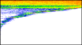
Sample index

EFlexics, $\kappa=0.9$

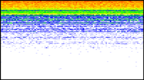
Sample index

Figure 4: The probability of observing a given item at a certain position in a batch by EFlexics is close to the expected probability of observing this item in a random itemset, which indicates high sampling accuracy. The samples by the lcm-based sampler are not exchangeable, i.e., certain items are under- or oversampled at certain positions in a batch, depending on their position in lcm’s search order.

Table 8: EFlexics generates individual samples considerably faster than lcm, although it is slower in counting. The kosarak dataset poses a significant challenge to EFlexics due to its number of items and sparsity that complicate the propagation of XOR constraints.

					Itemsets,	Counting, min			Sampling, s
	${\left|\mathcal{D}\right|}$	${\left|\mathcal{I}\right|}$	Density	$\theta$	bln.	lcm	EFlexics		lcm	EFlexics
accidents	$340183$	$469$	$\hphantom{3}7.21\%$	$0.009$	$\hphantom{1}5.37$	$1.55$	$6.48$		$33.77$	$10.30$
connect	$67557$	$130$	$33.08\%$	$0.178$	$16.88$	$0.01$	$0.38$		$59.00$	$0.37$
kosarak	$990002$	$41271$	$\hphantom{3}0.02\%$	$0.042$	$10.93$	$4.87$	$456.30$		$73.04$	$294.89$
pumsb	$49046$	$7117$	$\hphantom{3}1.04\%$	$0.145$	$\hphantom{1}1.11$	$0.09$	$1.19$		$18.14$	$0.75$

Table 8 summarizes the results. On three out of four datasets, lcm is faster in counting itemsets, but considerably slower in generating individual samples, which is even more pronounced on connect and pumsb than on accidents. The results are opposite on the kosarak dataset, which is in line with the theoretical expectations (see Section 5): the large number of items and the sparsity of the dataset sharply increase the costs of XOR constraint propagation. As a result, enumeration with Eclat within EFlexics becomes considerably slower than with lcm (augmenting lcm to handle XOR constraints might provide a solution, but is challenging from an implementation perspective).

Q4: Pattern set sampling In order to demonstrate the flexibility of our approach and the promised benefits of weighted constrained pattern sampling, i.e., 1) diversity and quality of results, 2) utility of constraints, and 3) the potential for anytime exploration, we here address the problem of sampling non-overlapping $2$-tilings as introduced in Section 6. We re-use the implementation of GFlexics from the itemset sampling experiments, only modifying the declarative specification of the CSP. Likewise, we impose the FCL constraints on constituent patterns.

Table 9 shows parameters and runtimes for sampling $2$-tilings proportional to $area$. The time to sample a single $2$-tiling is suitable for pattern-based data exploration, where tilings are inspected by a human user, as it exceeds $5$s only on the german dataset. For several settings, the estimation phase runtime slightly exceeds the runtime of enumerating all solutions. However, for the settings with a large number of pattern sets, which are arguably the primary target of pattern samplers, the opposite is true. For example, in the vote experiment with $170$ million tilings, the estimation phase runtime only amounts to $8\%$ of the complete enumeration runtime, which demonstrates the benefits of the proposed approach.

Table 9: Time required to sample a 2-tiling is approximately 4s, which is suitable for anytime exploration. Runtime benefits of the sampling procedure are the largest for the settings with the largest tiling counts (kr-vs-kp, primary, and vote).

						Sampling with GFlexics
	$\theta$	$\lambda$	Tilt	Tilings,	Enumeration,	Estimation,	Per sample,
			bound $\hat{r}$	mln.	min	min	s
german-credit	$0.22$	$3$	$25.4$	$11.2$	$8.2$	$12.6$	$15.3$
heart	$0.30$	$5$	$13.3$	$2.2$	$1.0$	$3.3$	$3.9$
hepatitis	$0.26$	$5$	$12.4$	$7.2$	$1.9$	$2.6$	$3.6$
kr-vs-kp	$0.31$	$4$	$13.1$	$20.3$	$18.5$	$3.5$	$5.1$
primary	$0.03$	$5$	$50.3$	$24.9$	$5.5$	$4.0$	$4.5$
vote	$0.10$	$5$	$15.3$	$170.1$	$37.0$	$2.9$	$4.4$

Tiling 1	Tiling 2
$area=1314$	$966$
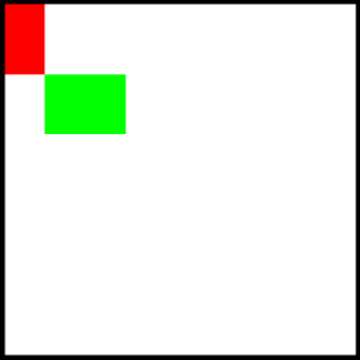
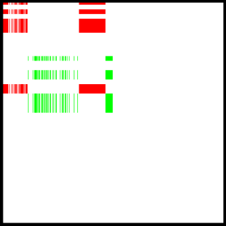
Tiling 3	Tiling 4
$941$	$878$
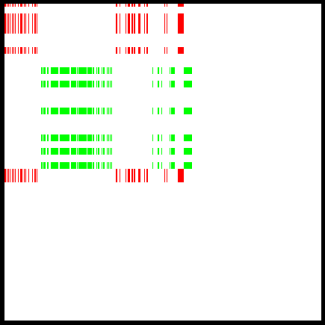
Tiling 5	Tiling 6
$799$	$765$

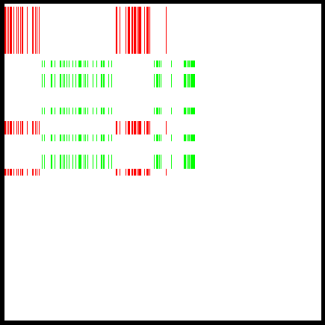
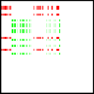
Figure 5: Left: Six 2-tilings sampled consecutively from the vote dataset. The tilings are diverse, i.e., cover different regions in the data, a property essential for pattern-based data exploration. (Note that while the sampled tilings are fair random draws, the images are not random: the tilings were sorted by $area$ descending, and items and transactions were re-arranged so that the cells covered by tilings with larger $area$ are as close to each other as possible.) Right: Qualities ($area$) of the samples, indicated by vertical bars, tend towards a dense region between the 25th and the 75th percentile.

The left part of Figure 5 shows six random $2$-tilings sampled from the vote dataset. Constraints ensure that the individual tiles comprising each $2$-tiling do not overlap, simplifying interpretation. Moreover, the set of tilings is diverse, i.e., the tilings are dissimilar to each other. They cover different regions in the data, revealing alternative structural regularities.

The right part of Figure 5 shows the $area$ distribution of all $2$-tilings that satisfy the constraints, obtained by complete enumeration. Qualities of 5 out of 6 tilings fall in the dense region between the $25$th and $75$th percentile, indicating high sampling accuracy. This is completely expected from the problem statement. In practice, pattern quality measures, like $area$, are only an approximation of application-specific pattern interestingness, thus diversity of results is a desirable characteristic of a pattern sampler as long as the quality of individual patterns is sufficiently high. To sample patterns from the right tail (i.e., with exceptionally high qualities) more frequently, the sampling task could be changed, e.g., either by choosing another sampling distribution or by enforcing constraints on $area$.

8 Discussion

The experiments demonstrate that Flexics delivers the promised benefits: 1) it is flexible in that it supports a wide range of pattern constraints and sampling distributions in itemset mining as well as the novel pattern set sampling task; 2) it is anytime in that the time it takes to generate random patterns is suitable for online data exploration, including the settings with large datasets or large solution spaces; and 3) by virtue of high sampling accuracy in all supported settings, sampled patterns are diverse, i.e., originate from different regions in the solution space. The theoretical guarantees ensure that the empirical observations extend reliably beyond the studied settings. Furthermore, practical accuracy is substantially higher than theory guarantees. The results confirm that pattern mining can benefit from the latest advances in AI, particularly in weighted constrained sampling for SAT. In this section, we discuss potential applications, advantages, and limitations of the proposed approach.

The primary application of pattern sampling involves showing sampled patterns directly to the user. In exploratory data analysis, the mining task is often ill-defined, i.e., the quality measure and the constraints reflect the application-specific pattern interestingness only approximately [34]. Owing to its flexibility, Flexics allows experimenting with various task formulations using the same algorithm. Pattern sampling allows obtaining diverse and representative sets of patterns in an anytime manner. These properties are particularly important in interactive mining systems, which aim at returning patterns that are subjectively interesting to the current user. Boley et al. [35] used two-step samplers in such a system, while Dzyuba and van Leeuwen [36] proposed to learn low-tilt subjective quality measures specifically for sampling with Flexics.

Furthermore, the theoretical guarantees enable applications beyond displaying the sampled patterns: Flexics can be plugged into algorithms that use patterns as building blocks for pattern-based models, yielding anytime versions thereof with $\left(\varepsilon,\delta\right)$-approximation guarantees of their own derived from Flexics’ guarantees. Example approaches include community detection with Eclat [37] or outlier detection with two-step sampling [38]. The authors note that the formulation of the mining task has a strong influence on the results in the respective applications. Flexics allows the algorithm designer to experiment with these choices and thus to obtain variants of these approaches, perhaps with better application performance.

The flexibility also provides algorithmic advantages. In addition to being agnostic of the quality measure $\varphi$ and the constraint set $\mathcal{C}$, Flexics is also agnostic of the underlying solution space and the oracle, as long as 1) solutions can be encoded with binary variables and 2) the oracle supports XOR constraints. Thus, Flexics provides a principled method to convert a pattern enumeration algorithm into a sampling algorithm, which amounts to implementing the mechanism to handle XOR constraints. This allows re-using algorithmic advances in pattern mining for developing pattern samplers, which we accomplished with cp4im and Eclat.

Most importantly, Flexics’ black-box nature simplifies extensions to new pattern languages. For example, possible extensions of GFlexics cover a variety of pattern set languages in Guns et al. [25], e.g., conceptual clustering. EFlexics can be extended to sample other binary pattern languages, e.g., association rules [1] or redescriptions [39]. In contrast, MCMC algorithms, like LRW, are based on local neighbourhood enumeration, which is uncommon in traditional pattern mining techniques, and thus require distinctive design and implementation principles for novel problems.

On the other hand, Flexics only supports pattern languages that can be compactly represented with binary variables, such as the itemsets and pattern sets studied in this paper. This essentially limits it to propositional discrete (binary, categorical, or discretized numeric) data. While in principle structured pattern languages, e.g., sequences or graphs, could also be modeled using this framework, the number of variables would rise sharply, which would negatively affect performance. Devising hashing-based sampling algorithms for non-binary domains is an open problem. In particular, sequence mining can be encoded with integer variables [26]; generalized XOR constraints [29] is one possible research direction. Alternatively, as the m4ri library [32] that we base our implementation on is optimized for dense $\mathbb{F}_{2}$ matrices, certain performance issues may be addressed with Gaussian elimination algorithms optimized for sparse matrices [40].

Another limitation concerns the bounded tilt assumption regarding sampling distributions: many common quality measures, e.g., $\chi^{2}$, information gain [41], or weighted relative accuracy [42], have high or even effectively infinite tilts (if $\varphi$ can be arbitrarily close to $0$). Such quality measures could be tackled with divide-and-conquer approaches [16, Section 6] or alternative estimation techniques [43]. This requires the capacity to efficiently handle constraints of the form $a\leq\varphi\left(p\right)\leq b$, which is possible for a number of quality measures, including the ones listed above.

9 Conclusion

We proposed Flexics, a flexible pattern sampler with theoretical guarantees regarding sampling accuracy. We leveraged the perspective on pattern mining as a constraint satisfaction problem and developed the first pattern sampling algorithm that builds upon the latest advances in sampling solutions in SAT. Experiments show that Flexics delivers the promised benefits regarding flexibility, efficiency, and sampling accuracy in itemset mining as well as in the novel task of pattern set sampling and that it is competitive with state-of-the-art alternatives.

Directions for future work include extensions to richer pattern languages and relaxing assumptions regarding sampling distributions (see Section 8 for a discussion). Specializing the sampling procedure towards typical mining scenarios may allow for deriving tighter theoretical bounds and improving the practical performance; examples include specific constraint types (e.g., anti-/monotone), shapes of sampling distributions (e.g., right-peaked distributions, similar to Figure 5), and iterative mining. Following the future developments in weighted constrained sampling in AI may provide insights for improving various aspects of Flexics or pattern sampling in general.

Acknowledgements The authors would like to thank Guy Van den Broeck for useful discussions and Martin Albrecht for the support with the m4ri library. Vladimir Dzyuba is supported by FWO-Vlaanderen.

Appendix A WeightGen

In this section, we present an extended technical description of the WeightGen algorithm, which closely follows Sections 3 and 4 in [16], whereas the pseudocode in Algorithm 2 is structured similarly to that of UniGen2, a close cousin of WeightGen [44]. Lines 3-5 correspond to the estimation phase and Lines 6-10 correspond to the sampling phase. SolveBounded stands for the bounded enumeration oracle.

The parameters of the estimation phase are fixed to particular theoretically motivated values. $pivot_{est}$ denotes the maximal weight of a cell at the estimation phase; $pivot_{est}=46$ corresponds to estimation error tolerance $\varepsilon_{est}=0.8$ (Line 14). If the total weight of solutions in a given cell exceeds $pivot_{est}$, a new random XOR constraint is added in order to eliminate a number of solutions. Repeating the process for a number of iterations increases the confidence of the estimate, e.g., $17$ iterations result in $1-\delta_{est}=0.8$ (Line 3). Note that Estimate essentially estimates the total weight of all solutions, from which $N_{XOR}$, the initial number of XOR constraints for the sampling phase, is derived (Line 6).

A similar procedure is employed at the sampling phase. It starts with $N_{XOR}$ constraints and adds at most three extra constraints. The user-chosen error tolerance parameter $\kappa$ determines the range $\left[loThresh,\ hiThresh\right]$, within which the total weight of a suitable cell should lie (Line 7). For example, $\kappa=0.9$ corresponds to range $\left[6.7,\ 49.4\right]$. If a suitable cell can be obtained, a solution is sampled exactly from all solutions in the cell; otherwise, no sample is returned. Requiring the total cell weight to exceed a particular value ensures the lower bound on the sampling accuracy.

The preceding presentation makes two simplifying assumptions: (1) all weights lie in $\left[1/r,\ 1\right]$; (2) adding XOR constraints never results in unsatisfiable subproblems (empty cells). The former is relaxed by multiplying pivots by $\hat{w}_{max}=\hat{w}_{min}\times\hat{r}<1$, where $\hat{w}_{min}$ is the smallest weight observed so far. The latter is solved by simply restarting an iteration with a newly generated set of constraints. See Chakraborty et al. [16] for the full explanation, including the precise formulae to compute all parameters.

Implementation details Following suggestions of Chakraborty et al. [44], we implement leapfrogging, a technique that improves the performance of the umbrella sampling procedure and thus benefits both GFlexics and EFlexics. First, after three iterations of the estimation phase, we initialize the following iterations with a number of XOR constraints that is equal to the smallest number returned in the previous iterations (rather than with zero XORs). Second, in the sampling phase, we start with one XOR constraint more than the number suggested by theory. If the cell is too small, we remove one constraint; if it is too large, we proceed adding (at most two) constraints. Both modifications are based on the observation that theoretical parameter values address hypothetical corner cases that rarely occur in practice. Finally, we only run the estimation phase until the initial number of XOR constraints, which only depends on the median of total weight estimates, converges. For example, if the estimation phase is supposed to run for 17 iterations, the convergence can happen as early as after 9 iterations.

Algorithm 2 WeightGen [16]

1:Boolean formula $F$, weight $w$, tilt bound $\hat{r}$, sampling error tolerance parameter $\kappa$

2:$w\left(\cdot\right)\in\left[1/\hat{r},\ 1\right]$, bounded enumeration algorithm SolveBounded

3:for $17$ iterations do $\triangleright$ Corresponds to $\delta_{est}=0.2$

4:     $WeightEstimates\overset{Add}{\leftarrow}$ Estimate($\emptyset$)

5:$TotalWeight=$ Median($WeightEstimates$)

6:$N_{XOR}=\mathcal{O}\left(\log_{2}TotalWeight/\left(1+\kappa^{-1}\right)\right)$

7:$loThresh\propto\left(1+\kappa\right)/\kappa^{2}$, $hiThresh\propto\left(1+\kappa\right)^{3}/\kappa^{2}$

8:for $N_{samples}$ times do

9:     $InitXORs$ = {RandomXOR() $\times N_{XOR}$ times}

10:     Generate($\kappa$, $\left[loThresh,\ hiThresh\right]$, $InitXORs$, $3$)

11:

12:function Estimate($XORs$)

13:$\triangleright$ Returns an estimate of the total weight of all solutions

14:     $pivot_{est}=46$ $\triangleright$ Corresponds to $\varepsilon_{est}=0.8$

15:     $Sols\leftarrow$ SolveBounded($F$, $XORs$, $pivot_{est}$)

16:     $CellWeight\leftarrow\sum_{s\in Sols}{w\left(s\right)}$

17:     if $CellWeight\leq pivot_{est}$ then $\triangleright$ Cell of the “right” size

18:         return $CellWeight\times 2^{{\left|XORs\right|}}$

19:     else$\triangleright$ Shrink cell by adding XOR constraint

20:         Estimate($XORs\ \cup$ RandomXOR())      

21:

22:function Generate($\kappa$, $\left[lT,\ hT\right]$, $XORs$, $i$)

23:$\triangleright$ Returns a random solution of $F$

24:     $Sols\leftarrow$ SolveBounded($F$, $XORs$, $hT$)

25:     $CellWeight\leftarrow\sum_{s\in Sols}{w\left(s\right)}$

26:     if $CellWeight\in\left[lT,\ hT\right]$ then $\triangleright$ Cell of the “right” size

27:         return SampleExactly($Sols$, $w$)

28:     else if $CellWeight>lT\land i>0$ then $\triangleright$ Cell is too large

29:         Generate($\kappa$, $\left[lT,\ hT\right]$, $XORs\cup\text{{RandomXOR}()}$, $i-1$)

30:     else$\triangleright$ Cell is too small

31:         return $\bot$

References

- [1] Rakesh Agrawal, Heikki Mannila, Ramakrishnan Srikant, Hannu Toivonen, and A. Inkeri Verkamo. Advances in Knowledge Discovery and Data Mining, chapter Fast Discovery of Association Rules, pages 307–328. 1996.
- [2] Charu C Aggarwal and Jiawei Han, editors. Frequent pattern mining. Springer International Publishing, 2014.
- [3] Toon Calders, Christophe Rigotti, and Jean-François Boulicaut. A survey on condensed representations for frequent sets. In Jean-François Boulicaut, Luc De Raedt, and Heikki Mannila, editors, Constraint-Based Mining and Inductive Databases, pages 64–80. Springer Berlin Heidelberg, 2006.
- [4] Albrecht Zimmermann and Siegfried Nijssen. Supervised pattern mining and applications to classification. In C. Charu Aggarwal and Jiawei Han, editors, Frequent Pattern Mining, chapter 17, pages 425–442. Springer International Publishing, 2014.
- [5] Siegfried Nijssen and Albrecht Zimmermann. Constraint-based pattern mining. In C. Charu Aggarwal and Jiawei Han, editors, Frequent Pattern Mining, chapter 7, pages 147–163. Springer International Publishing, 2014.
- [6] Björn Bringmann, Siegfried Nijssen, Nikolaj Tatti, Jilles Vreeken, and Albrecht Zimmermann. Mining sets of patterns. Tutorial at the European Conference on Machine Learning and Principles and Practice of Knowledge Discovery (ECML/PKDD ’10), 2010.
- [7] Mario Boley and Henrik Grosskreutz. Approximating the number of frequent sets in dense data. Knowledge and information systems, 21(1):65–89, 2009.
- [8] Mohammad Al Hasan and Mohammed J. Zaki. Output space sampling for graph patterns. Proceedings of the VLDB Endowment, 2(1):730–741, August 2009.
- [9] Mario Boley, Thomas Gärtner, and Henrik Grosskreutz. Formal concept sampling for counting and threshold-free local pattern mining. In Proceedings of the 10th SIAM International Conference on Data Mining (SDM ’10), pages 177–188, 2010.
- [10] Mario Boley, Claudio Lucchese, Daniel Paurat, and Thomas Gärtner. Direct local pattern sampling by efficient two-step random procedures. In Proceedings of the 17th ACM SIGKDD Conference on Knowledge Discovery and Data Mining (KDD ’11), pages 582–590, 2011.
- [11] Mario Boley, Sandy Moens, and Thomas Gärtner. Linear space direct pattern sampling using coupling from the past. In Proceedings of the 18th ACM SIGKDD Conference on Knowledge Discovery and Data Mining (KDD ’12), pages 69–77, 2012.
- [12] Carla P Gomes, Ashish Sabharwal, and Bart Selman. Near-uniform sampling of combinatorial spaces using XOR constraints. In Advances in Neural Information Processing Systems 19, pages 481–488. 2007.
- [13] Supratik Chakraborty, Kuldeep S Meel, and Moshe Y Vardi. A scalable and nearly uniform generator of SAT witnesses. In Proceedings of the 25th International Conference on Computer-Aided Verification (CAV ’13), pages 608–623, 2013.
- [14] Stefano Ermon, Carla P Gomes, Ashish Sabharwal, and Bart Selman. Embed and project: Discrete sampling with universal hashing. In Advances in Neural Information Processing Systems 26, pages 2085–2093. 2013.
- [15] Kuldeep Meel, Moshe Vardi, Supratik Chakraborty, Daniel Fremont, Sanjit Seshia, Dror Fried, Alexander Ivrii, and Sharad Malik. Constrained sampling and counting: Universal hashing meets SAT solving. In Proceedings of the Beyond NP AAAI Workshop, 2016.
- [16] Supratik Chakraborty, Daniel J Fremont, Kuldeep S Meel, and Moshe Y Vardi. Distribution-aware sampling and weighted model counting for SAT. In Proceedings of the 28th AAAI Conference on Artificial Intelligence (AAAI ’14), pages 1722–1730, 2014.
- [17] Tias Guns, Siegfried Nijssen, and Luc De Raedt. Itemset mining: A constraint programming perspective. Artificial Intelligence, 175(12-13):1951–1983, aug 2011.
- [18] Mohammed J. Zaki, Srinivasan Parthasarathy, Mitsunori Ogihara, and Wei Li. New algorithms for fast discovery of association rules. In Proceedings of the 3rd ACM SIGKDD Conference on Knowledge Discovery and Data Mining (KDD ’97), pages 283–296, 1997.
- [19] Jian Pei and Jiawei Han. Can we push more constraints into frequent pattern mining? In Proceedings of the 6th ACM SIGKDD Conference on Knowledge Discovery and Data Mining (KDD ’00), pages 350–354, 2000.
- [20] Arno Knobbe and Eric Ho. Pattern teams. In Proceedings of the 10th European Conference on Principles of Data Mining and Knowledge Discovery (PKDD ’06), pages 577–584, 2006.
- [21] Luc De Raedt and Albrecht Zimmermann. Constraint-based pattern set mining. In Proceedings of the 7th SIAM International Conference on Data Mining (SDM ’07), pages 237–248, 2007.
- [22] Cristian Bucilă, Johannes Gehrke, Daniel Kifer, and Walker White. Dualminer: A dual-pruning algorithm for itemsets with constraints. Data Mining and Knowledge Discovery, 7(3):241–272, 2003.
- [23] Francesco Bonchi, Fosca Giannotti, Claudio Lucchese, Salvatore Orlando, Raffaele Perego, and Roberto Trasarti. A constraint-based querying system for exploratory pattern discovery. Information Systems, 34(1):3–27, 2009.
- [24] Mehdi Khiari, Patrice Boizumault, and Bruno Crémilleux. Constraint programming for mining n-ary patterns. In Proceedings of the 16th International Conference on Principles and Practice of Constraint Programming (CP ’10), pages 552–567, 2010.
- [25] Tias Guns, Siegfried Nijssen, and Luc De Raedt. -pattern set mining under constraints. IEEE Transactions on Knowledge and Data Engineering, 25(2):402–418, 2013.
- [26] A Kemmar, W Ugarte, S Loudni, T Charnois, Y Lebbah, P Boizumault, and B Crémilleux. Mining relevant sequence patterns with CP-based framework. In Proceedings of the 26th IEEE International Conference on Tools with Artificial Intelligence (ICTAI ’14), pages 552–559, 2014.
- [27] Sergey Paramonov, Matthijs van Leeuwen, Marc Denecker, and Luc De Raedt. An exercise in declarative modeling for relational query mining. In Proceedings of the 25th International Conference on Inductive Logic Programming (ILP ’15), 2015.
- [28] Nino Shervashidze, SVN Vishwanathan, Tobias Petri, Kurt Mehlhorn, and Karsten M Borgwardt. Efficient graphlet kernels for large graph comparison. In Proceedings of the 12th International Conference on Artificial Intelligence and Statistics (AISTATS ’09), pages 488–495, 2009.
- [29] Carla P Gomes, Willem-jan van Hoeve, Ashish Sabharwal, and Bart Selman. Counting CSP solutions using generalized XOR constraints. In Proceedings of the 22nd AAAI Conference on Artificial Intelligence (AAAI ’07), pages 204–209, 2007.
- [30] Mate Soos. Enhanced gaussian elimination in DPLL-based SAT solvers. In Proceedings of the Pragmatics of SAT Workshop (POS ’10), pages 2–14, 2010.
- [31] Floris Geerts, Bart Goethals, and T Mielikäinen. Tiling databases. In Proceedings of the 7th International Conference on Discovery Science (DS ’04), pages 278–289, 2004.
- [32] Martin Albrecht and Gregory Bard. The M4RI Library. The M4RI Team, 2012.
- [33] Takeaki Uno, Masashi Kiyomi, and Hiroki Arimura. LCM ver. 3: Collaboration of array, bitmap and prefix tree for frequent itemset mining. In Proceedings of the 1st International Workshop on Open Source Data Mining: Frequent Pattern Mining Implementations (OSDM ’05), pages 77–86, 2005.
- [34] Deborah R Carvalho, Alex A Freitas, and Nelson Ebecken. Evaluating the correlation between objective rule interestingness measures and real human interest. In Proceedings of the 9th European Conference on Principles of Data Mining and Knowledge Discovery (PKDD ’05), pages 453–461, 2005.
- [35] Mario Boley, Michael Mampaey, Bo Kang, Pavel Tokmakov, and Stefan Wrobel. One Click Mining – interactive local pattern discovery through implicit preference and performance learning. In Proceedings of the ACM SIGKDD Workshop on Interactive Data Exploration and Analytics (IDEA ’13), pages 28–36, 2013.
- [36] Vladimir Dzyuba and Matthijs van Leeuwen. Learning what matters – sampling interesting patterns. In Proceedings of the 21st Pacific-Asia Conference on Knowledge Discovery and Data Mining (PAKDD ’17), 2017. in press.
- [37] Michele Berlingerio, Fabio Pinelli, and Francesco Calabrese. ABACUS: Frequent pattern mining-based community discovery in multidimensional networks. Data Mining and Knowledge Discovery, 27(3):294–320, 2013.
- [38] Arnaud Giacometti and Arnaud Soulet. Anytime algorithm for frequent pattern outlier detection. International Journal of Data Science and Analytics, 2(3):119–130, 2016.
- [39] Naren Ramakrishnan, Deept Kumar, Bud Mishra, Malcolm Potts, and Richard Helm. Turning CARTwheels: an alternating algorithm for mining redescriptions. In Proceedings of the 10th ACM SIGKDD Conference on Knowledge Discovery and Data Mining (KDD ’04), pages 266–275, 2004.
- [40] Charles Bouillaguet and Claire Delaplace. Sparse gaussian elimination modulo : An update. In Proceedings of the 18th International Workshop on Computer Algebra in Scientific Computing (CASC ’16), pages 101–116, 2016.
- [41] Siegfried Nijssen, Tias Guns, and Luc De Raedt. Correlated itemset mining in ROC space: A constraint programming approach. In Proceedings of the 15th ACM SIGKDD Conference on Knowledge Discovery and Data Mining (KDD ’09), pages 647–655, 2009.
- [42] Florian Lemmerich, Martin Becker, and Frank Puppe. Difference-based estimates for generalization-aware subgroup discovery. In Proceedings of the European Conference on Machine Learning and Principles and Practice of Knowledge Discovery (ECML/PKDD ’13), pages 288–303, 2013.
- [43] Stefano Ermon, Carla P. Gomes, Ashish Sabharwal, and Bart Selman. Taming the curse of dimensionality: Discrete integration by hashing and optimization. In Proceedings of the 30th International Conference on Machine Learning (ICML ’13), pages 334–342, 2013.
- [44] Supratik Chakraborty, Daniel J. Fremont, Kuldeep S. Meel, Sanjit A. Seshia, and Moshe Y. Vardi. On parallel scalable uniform SAT witness generation. In Proceedings of the 21st International Conference on Tools and Algorithms for the Construction and Analysis of Systems (TACAS ’15), volume 9035, pages 304–319, 2015.