Perturbations of spiky strings in flat spacetimes

Abstract:

Perturbations of a class of semiclassical strings known today as spiky strings, are studied using the well-known Jacobi equations for small normal deformations of an embedded timelike surface. It is shown that there exists finite normal perturbations of the spiky string worldsheets embedded in a $2+1$ dimensional flat spacetime. Such perturbations lead to a rounding off of the spikes, which, in a way, demonstrates the stable nature of the unperturbed worldsheet. The same features appear for the dual spiky string solution and in the spiky as well as their dual solutions in $3+1$ dimensional flat spacetime. Our results are based on exact solutions of the corresponding Jacobi equations which we obtain and use while constructing the profiles of the perturbed configurations.

1 Introduction

Rigidly rotating strings were first proposed by Burden and Tassie in 1982 [1, 2] and explored further in the next few years in a series of papers [3, 4]. Later, Embacher [5] obtained the complete class of cosmic string solutions in flat spacetime that undergo rigid rotation about a fixed axis. Subsequent work, by various authors, on such string configurations have appeared in [6, 7, 8]. More recently, in [9], Burden has come up with additional comments on the work reported in [10].

In the context of AdS/CFT correspondence [11], the spiky string solutions have re-appeared, through the seminal work by Kruczenski [12], as a potential gravity dual to higher twist operators in string theory. The focus, in string theory, however, has been on the solutions which are closed strings with spikes (in cosmic string nomenclature these are known as cusps). The ‘semiclassicality’ of these solutions is argued from the evaluation of the energies and angular momenta of such spiky string configurations [13]. From the AdS₅/CFT₄ perspective, as mentioned above, the spiky strings are special because they correspond to certain higher twist operators in ${\cal N}$ =4 Supersymmetric Yang Mills (SYM) theory. Further, these spiky strings have been found to be a special class of the general rigidly rotating strings. In proving AdS/CFT duality, the appearance of so-called ${\it integrability}$ at the level of the classical string worldsheet [14], [15] as well as in N=4 gauge theory [16] has played a key role. The semiclassical string states in the gravity side have been used to look for suitable gauge theory operators on the boundary, in establishing the duality. In this connection, Hoffman and Maldacena (HM) considered a special limit $(J\rightarrow\infty$, $\lambda$ = fixed, $p$ = fixed, $E-J$ = fixed), with $J$ being the angular momentum, $E$ the total energy, $p$ the momentum carried by the string in the spin chain and $\lambda$ the ‘t Hooft coupling constant. In this limit, the problem of determining the spectrum on both (i.e. string and gauge theory) sides becomes simple. The spectrum consists of an elementary excitation known as magnon which propagates with a conserved momentum $p$ along the spin chain. Further, a general class of rigidly rotating string solutions in $AdS_{5}\times S^{5}$ is the spiky string which describes the higher twist operators from the dual field theory viewpoint. giant magnons can be visualised as a special limit of such spiky strings with shorter wavelengths. A large class of such spiky strings in various asympotically AdS and non-AdS backgrounds have been studied in the literature [12],[17],[18],[19],[20],[21],[22].

Therefore, it is interesting to look at the geometric properties of such string configurations from the world sheet view point and study normal perturbations (linearized) around the classical solutions. In this connection, for the case of rotating superstrings there has been studies [23] on computation of leading quantum corrections to the energy spectrum by expanding the supersymmetric action to quadratic order in fluctuations near the classical solution. In flat spacetime, where the string action is Gaussian in the conformal gauge, this would account for the full string spectrum of states no matter what classical solutions one starts with.

In this article, we investigate the classical stability of the spiky strings using the well-known Jacobi equations [24],[25],[26], [27] which govern normal deformations of an embedded surface. Recent work on such perturbations can be found in [28]. We choose to first work with the simplest spiky strings–the Kruczenski solution in flat spacetime in $2+1$ dimensions and generalize it further to $3+1$ dimensions. The rest of the paper is organised as follows. In section 2, we briefly summarize the solutions and the two different embeddings of the worldsheet that will be used in our analysis of perturbations. Section 3 is devoted to study of the perturbation equations, their solutions and the perturbed profiles, with illustrative examples. The straightforward extension to a flat background in $3+1$ dimensions is discussed in Section 4. Concluding remarks appear in Section 5.

2 Spiky strings in $2+1$ dimensions: the Kruczenski and Jevicki-Jin embeddings

The Nambu-Goto action for the bosonic string embedded in an arbitrary $N$ dimensional curved background spacetime with metric functions $g_{ij}(x)$, is given as

$$S=-T\int d\tau\,\,d\sigma\sqrt{-\gamma}=-T\int d\tau\,\,d\sigma\sqrt{(\dot{x}\cdot x^{\prime})^{2}-\dot{x}^{2}{x^{\prime}}^{2}}\ .$$ (1)

where $\gamma$ is the determinant of the induced metric $\gamma_{ab}=g_{ij}\partial_{a}x^{i}\partial_{b}x^{j}$ ($a,b=\sigma,\tau$);   $x^{i}(\tau,\sigma)$ the embedding functions and $T$ the string tension. We have denoted $\dot{x}=\partial_{\tau}x$,  $x^{\prime}=\partial_{\sigma}x$,   $(\dot{x}\cdot x^{\prime})=g_{ij}{\dot{x}}^{i}\,{x^{\prime}}^{j}$,  ${\dot{x}}^{2}=g_{ij}{\dot{x}}^{i}\,{\dot{x}}^{j}$ and ${x^{\prime}}^{2}=g_{ij}{x^{\prime}}^{i}\,{x^{\prime}}^{j}$.

Choosing a conformal gauge in which the induced metric is diagonal, we have

$$g_{ij}({\dot{x}}^{i}{\dot{x}}^{j}+{x^{\prime}}^{i}{x^{\prime}}^{j})=0,\hskip 21.68121ptg_{ij}{\dot{x}}^{i}{x^{\prime}}^{j}=0\ .$$ (2)

In this conformal gauge, the string equations of motion obtained by varying the action w.r.t. $x^{\mu}$, take the form:

$${\ddot{x}}^{i}-{x^{i^{\prime\prime}}}+\Gamma^{i}_{jk}\left({\dot{x}}^{j}{\dot{x}}^{k}-{x}^{j\prime}{x}^{k\prime}\right)=0\ .$$ (3)

We first consider a $2+1$ dimensional flat background spacetime with a line element (in $t,\rho,\theta$ coordinates) given as:

$$ds^{2}=-dt^{2}+d\rho^{2}+\rho^{2}d\theta^{2}\ .$$ (4)

There are various choices for embeddings which may be used to obtain string worldsheets which satisfy the string equations of motion (3) and the Virasoro constraints (2). Denoting $\tau$ and $\sigma$ as worldsheet coordinates we may choose the following embedding due to Jevicki and Jin [29]:

$$t=\tau+f(\sigma),\hskip 7.22743pt\rho=\rho(\sigma),\hskip 7.22743pt\theta=\omega\tau+g(\sigma)\ .$$ (5)

Using the above ansatz in the string equations of motion and constraints, we arrive at the following equations of motion

$$f^{\prime\prime}=0,\hskip 14.45377pt\rho^{\prime\prime}+\rho\left(\omega^{2}-{g^{\prime}}^{2}\right)=0$$ (6)

$$g^{\prime\prime}+2\frac{\rho^{\prime}}{\rho}g^{\prime}=0$$ (7)

and constraints

$$-(1+f^{\prime 2})+{\rho^{\prime}}^{2}+\rho^{2}\left(\omega^{2}+{g^{\prime}}^{2}\right)=0,\hskip 14.45377ptf^{\prime}=\rho^{2}\omega g^{\prime}.$$ (8)

The first integrals of the above equations are:

$$f^{\prime}=\bar{a},\hskip 14.45377ptg^{\prime}=\frac{\bar{a}}{\omega\rho^{2}}$$ (9)

$${\rho^{\prime}}^{2}=\left(1-\rho^{2}\omega^{2}\right)\left(1-\frac{{\bar{a}}^{2}}{\omega^{2}\rho^{2}}\right)$$ (10)

A further integration finally yields the functions $\rho(\sigma)$, $f(\sigma)$ and $g(\sigma)$ and we get

$$t=\tau+{\bar{a}}\left(\sigma-\sigma_{0}\right),\>\>\>\rho=\frac{1}{\omega}\left[{\bar{a}}^{2}+(1-{\bar{a}}^{2})\sin^{2}\omega(\sigma-\sigma_{0})\right]^{\frac{1}{2}},$$

$$\theta=\omega\tau+\tan^{-1}\left[\frac{1}{\bar{a}}\tan\{\omega(\sigma-\sigma_{0})\}\right]\$$

where $0<\bar{a}<1$ and $\sigma_{0}$ are constants.

Let us now convert this solution to Cartesian coordinates which will enable us to plot the profiles of the unperturbed and perturbed string worldsheets at fixed values of $\tau$. To do this we need to use certain coordinate transformations and also some definitions. We will work with $\sigma_{0}=0$. The $\omega\sigma_{0}=\frac{\pi}{2}$ case can also be worked out easily. We define $\rho_{0}$ and $\rho_{1}$ as follows:

$$\rho_{1}=\frac{1}{\omega},\hskip 7.22743pt\rho_{0}=\frac{\bar{a}}{\omega}\ ,$$ (12)

where $\rho_{0}$ and $\rho_{1}$ are the minimum and maximum values of the function $\rho(\sigma)$. Spikes occur at $\rho_{1}$ whereas $\rho_{0}$ correspond to valleys. To go over to Cartesian coordinates we write $x=\rho\cos\theta$, $y=\rho\sin\theta$ and then use new worldsheet coordinates ($\tau^{\prime}$ and $\sigma^{\prime}$) via a coordinate transformation. As noted by Kruczenski [12] the coordinate transformation is given as

$$\tau=-\frac{\rho_{1}^{2}}{\rho_{0}-\rho_{1}}\tau^{\prime}-\frac{\rho_{0}\rho_{1}}{\rho_{0}-\rho_{1}}\sigma^{\prime},\hskip 14.45377pt\sigma=\frac{\rho_{1}\rho_{0}}{\rho_{0}-\rho_{1}}\tau^{\prime}+\frac{\rho_{1}^{2}}{\rho_{0}-\rho_{1}}\sigma^{\prime}\ .$$ (13)

Further we define

$$\frac{\rho_{1}-\rho_{0}}{\rho_{1}+\rho_{0}}=\frac{1}{n-1}\ ,$$ (14)

and note that

$$\bar{a}=\frac{n-2}{n},\hskip 14.45377pt\omega=\frac{1}{\rho_{1}}\ .$$ (15)

If we rewrite $\rho$ and $\theta$ using the above definitions we see that there are $n$ spikes over the range $0$ to $2\pi$ of $\sigma^{\prime}$. The coordinate transformations and the definitions given above eventually yield the Cartesian embedding functions as functions of $\tau^{\prime}$ and $\sigma^{\prime}$, given as

$$x=\frac{\rho_{0}}{n-2}\left[(n-1)\cos\left(\tau^{\prime}-\sigma^{\prime}\right)-\cos\{(n-1)\left(\tau^{\prime}+\sigma^{\prime}\right)\}\right]\ ,$$

$$y=\frac{\rho_{0}}{n-2}\left[(n-1)\sin\left(\tau^{\prime}-\sigma^{\prime}\right)-\sin\{(n-1)\left(\tau^{\prime}+\sigma^{\prime}\right)\}\right]\ ,$$ (16)

with $t$ proportional to $\tau^{\prime}$. We will make use of both the embeddings in order to understand the perturbations. As mentioned before, if we use $\omega\sigma_{0}=\frac{\pi}{2}$ we will get back, in Cartesian coordinates, the exact forms given by Kruczenski [12].

3 Perturbations of spiky strings in $2+1$ dimensions

Before we embark on writing down the perturbation equations for our specific solutions, we review the main results on the perturbations of extremal worldsheets.

3.1 Perturbation equations for extremal worldsheets

Assuming (as before) $x^{i}(\tau,\sigma)$ as the embedding functions and $g_{ij}$ as the background metric, the tangent vectors to the worldsheet are defined as

$$e^{i}_{\tau}=\partial_{\tau}x^{i},\hskip 14.45377pte^{i}_{\sigma}=\partial_{\sigma}x^{i},$$ (17)

The induced line element is

$$\gamma_{ab}=g_{ij}e^{i}_{a}e^{j}_{b}\ ,$$ (18)

where the $a,b...$ denote worldsheet indices (here $\tau$, $\sigma$). The normals to the worldsheet $n^{i}_{(\alpha)}$ satisfy the following relations

$$g_{ij}n^{i}_{(\alpha)}n^{j}_{(\beta)}=\delta_{\alpha\beta},\hskip 14.45377ptg_{ij}n^{i}_{(\alpha)}e^{j}_{a}=0\ ,$$ (19)

where $\alpha=1..,N-2$ where $N$ is the dimension of the background spacetime. The last condition is valid for all $\alpha$ and $a$. The extrinsic curvature tensors $K_{ab}^{(\alpha)}$ along each normal $n^{i}_{(\alpha)}$ of the embedded worldsheet are defined as

$$K_{ab}^{(\alpha)}=-g_{ij}(e^{k}_{a}\nabla_{k}e^{i}_{b})n^{j(\alpha)}\ .$$ (20)

One can check that the equations of motion correspond to the condition that $K^{(\alpha)}=\gamma^{ab}K_{ab}^{(\alpha)}=0$ which means that the worldsheet is an extremal surface with zero value for the trace of each extrinsic curvature tensor. Normal perturbations are defined using a set of scalar fields $\phi^{(\alpha)}$ along each normal. We have

$$\delta x^{i}=\phi^{(\alpha)}n^{i}_{(\alpha)}\ ,$$ (21)

as the resultant perturbation of the worldsheet (i.e. $x^{i}\rightarrow x^{i}+\delta x^{i}$). For an extremal worldsheet ($\gamma^{ab}K_{ab}^{(\alpha)}=0$) satisfying the equations of motion and the Virasoro constraints, the scalars $\phi^{i}_{(\alpha)}$ satisfy the following equations (Jacobi equations) which follow from the second variation of the Nambu-Goto action.

$$\frac{1}{\Omega^{2}}\left(-\frac{\partial^{2}}{\partial\tau^{2}}+\frac{\partial^{2}}{\partial\sigma^{2}}\right)\phi^{(\alpha)}+\left(M^{2}\right)^{(\alpha)}_{(\beta)}\phi^{(\beta)}=0\ ,$$ (22)

where

$$\left(M^{2}\right)^{(\alpha)}_{(\beta)}=K_{ab}^{(\alpha)}K^{ab}_{(\beta)}+R_{ijkl}e^{j}_{a}e^{l\,\,a}n^{i\,\,(\alpha)}n^{k}_{(\beta)}\ ,$$ (23)

and $\Omega^{2}(\tau,\sigma)$ is the conformal factor of the conformally flat worldsheet line element. Solving this equation for the perturbation scalars one can learn about the stability of the extremal worldsheet under perturbations. Note that the Jacobi equations turn out to be a family of coupled variable ‘mass’ wave equations for the perturbation scalars $\phi^{(\alpha)}$. In general, they are difficult to solve exactly, even for the simplest cases. However, fortunately, for the cases discussed below we do find exact solutions quite easily.

We may also note the fact that, in general, the worldsheet covariant derivative (which arises in the first term in Eqn. 3.6) can have a contribution from the normal fundamental form (extrinsic twist potential) defined as $\omega_{a}^{\,\,\alpha\beta}=g_{ij}\,\left(e^{k}_{a}\nabla_{k}\,n^{i\,\alpha}\right)\,n^{j\,\beta}$. However, for hypersurfaces and for the normals considered in the $3+1$ dimensional case to be discussed later, the $\omega_{a}^{\alpha\beta}$ are identically zero.

3.2 The case of spiky strings

In order to find the perturbation equations for our case we need to first write down the tangent, normal, induced metric and extrinsic curvature for the world sheet. Here, we use the Jevicki-Jin embedding mentioned earlier. The tangent vector to the worldsheet is given as:

$$e^{i}_{\tau}=\left(1,0,\omega\right),\hskip 14.45377pte^{i}_{\sigma}=\left(f^{\prime},\rho^{\prime},g^{\prime}\right)\ .$$ (24)

Using the expressions for $f$, $g$ and $\rho$ quoted earlier the induced line element turns out to be

$$ds^{2}=\left(1-\rho^{2}\omega^{2}\right)\left(-d\tau^{2}+d\sigma^{2}\right)\ .$$ (25)

The normal to the worldsheet is given as:

$$n^{i}=\left(\tan\omega\sigma,-\frac{\bar{a}}{\omega\rho},\frac{\tan\omega\sigma}{\omega\rho^{2}}\right)\ .$$ (26)

The extrinsic curvature tensor turns out to be

$$K_{ab}=\begin{pmatrix}-\bar{a}\omega&-\omega\cr-\omega&-\bar{a}\omega\end{pmatrix}\ .$$ (27)

Hence the quantity $K_{ab}K^{ab}$ is given as:

$$K_{ab}K^{ab}=-\frac{2\omega^{2}(1-\bar{a}^{2})}{(1-\rho^{2}\omega^{2})^{2}}=-{}^{2}R\ ,$$ (28)

where ${}^{2}R$ is the worldsheet Ricci scalar. Given that $\bar{a}<1$, we note that ${}^{2}R$ is positive and blows up to positive infinity at the location of the spikes, i.e. wherever $\rho^{2}\omega^{2}=1$.

Since the background is flat the Riemann tensor is zero and, therefore, the equation for the perturbation scalar (here only one scalar because there is only one normal) turns out to be:

$$\left(-\frac{\partial^{2}}{\partial\tau^{2}}+\frac{\partial^{2}}{\partial\sigma^{2}}\right)\phi-\frac{2\omega^{2}(1-\bar{a}^{2})}{(1-\rho^{2}\omega^{2})^{2}}\phi=0\ .$$ (29)

Using the functional form of $\rho(\sigma)$ one can reduce this equation to

$$\left(-\frac{\partial^{2}}{\partial\tau^{2}}+\frac{\partial^{2}}{\partial\sigma^{2}}\right)\phi-2\omega^{2}\sec^{2}\omega\sigma\phi=0\ .$$ (30)

Let us take a simple separable ansatz of the form

$$\phi=e^{i\beta\tau}P(\sigma)\ .$$ (31)

We end up with an equation for $P(\sigma)$ given as

$$\frac{d^{2}P}{d\sigma^{2}}+\left(\beta^{2}-2\omega^{2}\sec^{2}\omega\sigma\right)P=0\ .$$ (32)

A simple transformation $\xi=\omega\sigma$ reduces this equation to

$$\frac{d^{2}P}{d\xi^{2}}+\left(\gamma^{2}-2\sec^{2}\xi\right)P=0$$ (33)

where $\beta=\gamma\omega$. It turns out that this is an equation which we encounter in quantum mechanical potential problems–a special case of the well-known Poschl-Teller potential [30]. One can surely solve this equation exactly but before we do that let us try and look at a simple and obvious solution. For $\gamma=2$ we have a solution for $P(\xi)$ given as

$$P(\xi)=\epsilon\rho_{0}\cos^{2}\xi\ ,$$ (34)

where $\epsilon$ is a constant and we may relate it to the amplitude of the perturbation. It must be emphasized that $\epsilon$ has to be small in value (i.e. $\epsilon<<1$) in order that the deformation is genuinely a perturbation. This also follows from the relative magnitudes of the two terms in the expression for $\rho^{\prime}$ below. Since the minimum value of $\rho$ is $\rho_{0}$ and the perturbation goes as $\epsilon\rho_{0}$, one ie required to have $\epsilon<<1$. More generally, the Jacobi equations are not even valid equations for the perturbations when the perturbations themselves become large.

Let us now write down the perturbations for this mode (the abovestated $\gamma=2$ solution $P(\xi)$). For the $\tau$ part of the full solution we take its real part (i.e. $\cos\beta\tau=\cos 2\omega\tau$). One may also work with the imaginary part. We find

$$t^{\prime}=t+\phi n^{0}=t+\epsilon\rho_{0}\cos 2\omega\tau\sin\omega\sigma\cos\omega\sigma,$$

$$\rho^{\prime}=\rho+n^{1}\phi=\rho-\epsilon\rho_{0}\frac{\bar{a}\cos 2\omega\tau\cos^{2}\omega\sigma}{\sqrt{{\bar{a}}^{2}+(1-{\bar{a}}^{2})\sin^{2}\omega\sigma}},$$

$$\theta^{\prime}=\theta+n^{2}\phi=\theta+\epsilon\rho_{0}\frac{\omega\cos 2\omega\tau\sin\omega\sigma\cos\omega\sigma}{{\bar{a}}^{2}+(1-{\bar{a}}^{2})\sin^{2}\omega\sigma}\ .$$

Let us now try to understand how this perturbation affects the string profile. We need to switch back to Cartesian coordinates to get a clearer picture here. Defining $x^{\prime}=\rho^{\prime}\cos\theta^{\prime}$ and $y^{\prime}=\rho^{\prime}\sin\theta^{\prime}$ we use $\rho^{\prime}=\rho+\delta\rho$ and $\theta^{\prime}=\theta+\delta\theta$ to eventually obtain

$$t^{\prime}=t+\delta t,\>\>\>x^{\prime}=x+\frac{\delta\rho}{\rho}\,\,x-\delta\theta\,\,y\ ,\>\>\>y^{\prime}=y+\frac{\delta\rho}{\rho}\,\,y+\delta\theta\,\,x\ .$$ (36)

In the above expressions, we will now substitute $\delta t$, $\frac{\delta\rho}{\rho}$, $\delta\theta$ and switch back to the $(\tau^{\prime},\sigma^{\prime})$ coordinates on the worldsheet. Thereafter, taking small values of $\epsilon$ we will obtain the perturbed worldsheet and compare it with the unperturbed worldsheet. This will help us get an idea of what the normal perturbations do to the spiky string.

Let us begin with the solutions for $P(\xi)$. For $\gamma=2$ we have noted above that $P(\xi)=\epsilon\rho_{0}\cos^{2}\xi$ is a solution. The other linearly independent solution has an overall $\sec\xi$ and is divergent. This feature persists for all pairs of linearly independent solutions for different values of $\gamma$. We have one oscillatory solution and another divergent solution. We can write the general solutions using hypergeometric functions (see details later). We now move on to writing down $\delta t$, $\frac{\delta\rho}{\rho}$ and $\delta\theta$ using the $(\tau^{\prime},\sigma^{\prime})$ coordinates for the $P(\xi)=\epsilon\rho_{0}\cos^{2}\xi$ solution with $\gamma=2$. This gives

$$\delta t=\frac{\epsilon\rho_{0}}{4}\left[\sin 2(\tau^{\prime}-\sigma^{\prime})-\sin 2(n-1)(\tau^{\prime}-\sigma^{\prime})\right]$$ (37)

$$\frac{\delta\rho}{\rho}=-\epsilon\frac{(n-2)^{2}\cos\{n\tau^{\prime}+(n-2)\sigma^{\prime}\}\cos^{2}\{\frac{n-2}{2}\tau^{\prime}+\frac{n}{2}\sigma^{\prime}\}}{(n-2)^{2}+4(n-1)\sin^{2}\{\frac{n-2}{2}\tau^{\prime}+\frac{n}{2}\sigma^{\prime}\}}$$ (38)

$$\delta\theta=-\epsilon\frac{n(n-2)\cos\{n\tau^{\prime}+(n-2)\sigma^{\prime}\}\cos\{\frac{n-2}{2}\tau^{\prime}+\frac{n}{2}\sigma^{\prime}\}\sin\{\frac{n-2}{2}\tau^{\prime}+\frac{n}{2}\sigma^{\prime}\}}{(n-2)^{2}+4(n-1)\sin^{2}\{\frac{n-2}{2}\tau^{\prime}+\frac{n}{2}\sigma^{\prime}\}}\ .$$ (39)

These expressions can now be substituted in those for $t^{\prime}$, $x^{\prime}$, $y^{\prime}$ in order to obtain the perturbed worldsheet. The simplest case is with $n=3$. Here, we have $t^{\prime}$, $x^{\prime}$ and $y^{\prime}$ as follows.

$$t^{\prime}=4\tau^{\prime}+\frac{\epsilon\rho_{0}}{4}\left[\sin[2(\tau^{\prime}-\sigma^{\prime})]-\sin[4(\tau^{\prime}+\sigma^{\prime})]\right]\ ,$$ (40)

$$x^{\prime}=A(\tau^{\prime},\sigma^{\prime})\,\,x+B(\tau^{\prime},\sigma^{\prime})\,\,y\ ,$$ (41)

$$y^{\prime}=-B(\tau^{\prime},\sigma^{\prime})\,\,x+A(\tau^{\prime},\sigma^{\prime})\,\,y\ ,$$ (42)

where

$$A(\tau^{\prime},\sigma^{\prime})=\left(1-\epsilon\frac{\cos(\sigma^{\prime}+3\tau^{\prime})\cos^{2}(\frac{3\sigma^{\prime}}{2}+\frac{\tau^{\prime}}{2})}{1+8\sin^{2}(\frac{3\sigma^{\prime}}{2}+\frac{\tau^{\prime}}{2})}\right)$$ (43)

$$B(\tau^{\prime},\sigma^{\prime})=\left(\epsilon\frac{3\cos(\sigma^{\prime}+3\tau^{\prime})\sin(\frac{3\sigma^{\prime}}{2}+\frac{\tau^{\prime}}{2})\cos(\frac{3\sigma^{\prime}}{2}+\frac{\tau^{\prime}}{2})}{1+8\sin^{2}(\frac{3\sigma^{\prime}}{2}+\frac{\tau^{\prime}}{2})}\right)$$ (44)

and $x$ and $y$ are given as

$$x=2\cos(\tau^{\prime}-\sigma^{\prime})-\cos 2(\tau^{\prime}+\sigma^{\prime})\ ,\>\>\>y=2\sin(\tau^{\prime}-\sigma^{\prime})-\sin 2(\tau^{\prime}+\sigma^{\prime})\ .$$

Note that, in writing down the above an overall factor of $\rho_{0}$ has been scaled out in the definition of the coordinates.

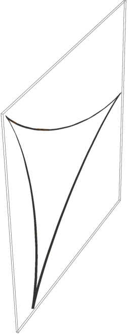
Figure 1: $n=3$, $\tau^{\prime}\equiv(4.0,4.01)$, unperturbed.

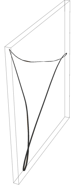
Figure 2: $n=3$, $\epsilon=0.2$, $\tau^{\prime}\equiv(4.0,4.01)$, perturbed.

Figures 1-6 demonstrate the scenario for $n=3$. Figure 1 shows the worldsheet over a small range of $\tau^{\prime}$ (i.e. $\tau^{\prime}=4.0$ to $\tau^{\prime}=4.01$). One can see the three spikes. The very slight rigid rotation of the profile along $\tau^{\prime}$ is visible through the thickened character of the black lines. Figure 2 represents the perturbed worldsheet profile for the same range of $\tau^{\prime}$. One notices that the worldsheet is now spread across the $t^{\prime}$ direction because $t^{\prime}$ is dependent on both $\tau^{\prime}$ and $\sigma^{\prime}$. In Figure 2, the spikes are rounded off and the string spreads out– there are no self-intersections. Figure 3 shows the worldsheet profile near the spikes whereas Figure 4 shows how a spike location gets rounded off due to the perturbation. Thus, the effect of the perturbation seems to be in rounding off the spikes. Similar observations were made in the presence of large angular momentum in [19], [31].

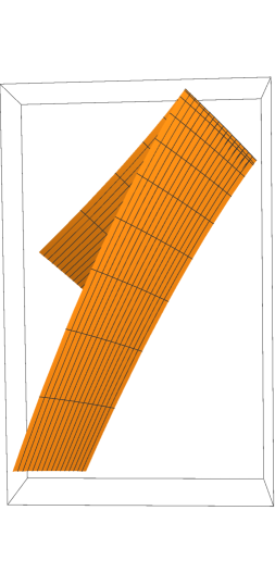
Figure 3: $n=3$, unperturbed, $\tau^{\prime}\equiv(4.0,4.05)$, $\sigma^{\prime}\equiv(0.4\pi,0.7\pi)$.

Figure 4: $n=3$, perturbed, $\epsilon=0.24$, $\tau^{\prime}\equiv(4.0,4.05)$, $\sigma^{\prime}\equiv(0.5\pi,0.7\pi)$.

It is easy to repeat the above calculation to obtain the other modes. Here too we have found similar features. We do not discuss them in any further detail.

The general solutions of the second order differential equation for $P$ can be written as a superposition of the two linearly independent ones, both of which involve hypergeometric functions. Note that the differential equation is a special case of the well-known Poschl-Teller potential problem in quantum mechanics [30]. We can write

$$P(\xi)=C_{1}P_{1}+C_{2}P_{2}\ ,$$ (46)

where the $P_{1}$ and $P_{2}$ are given by

$$P_{1}=\epsilon\cos^{2}{\xi}\,\,{}_{2}F_{1}(\frac{2+\gamma}{2},\frac{2-\gamma}{2},\frac{1}{2};\sin^{2}{\xi})\ ,$$ (47)

$$P_{2}=\epsilon\sin{\xi}\cos^{2}{\xi}\,\,{}_{2}F_{1}(\frac{3+\gamma}{2},\frac{3-\gamma}{2},\frac{3}{2};\sin^{2}{\xi})$$ (48)

where

$$\gamma=2+2\nu,\hskip 14.45377pt\nu=0,1,2.....\ .$$ (49)

Each allowed value of $\nu$ yields the corresponding fluctuation mode of a given configuration. As before, we include here the $\epsilon$, which is the amplitude of the perturbation. For every allowed value of $\gamma$, $P_{1}$ represents an oscillatory solution whereas $P_{2}$ is a divergent solution.

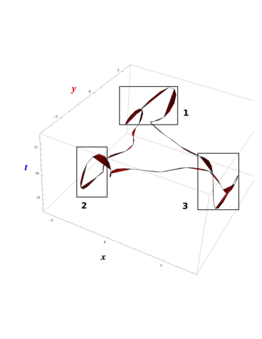
Figure 5: $n=3$ , $\gamma=4$ , $\tau^{\prime}\equiv(4,4.01)$, $\epsilon=0.1$, $\sigma^{\prime}\equiv(0,2\pi)$.

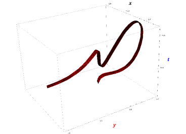
Figure 6: Region $1$ in Fig. 5, $n=3$ , $\gamma=4$ , $\tau^{\prime}\equiv(4,4.01)$, $\epsilon=0.1$,$\sigma^{\prime}\equiv(\frac{\pi}{3},0.8\pi)$.

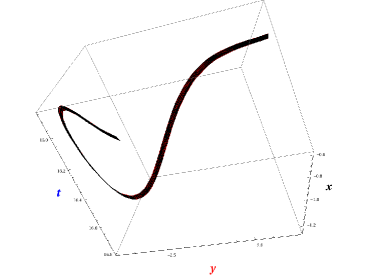
Figure 7: Region $2$ in Fig. 5, $n=3$ , $\gamma=4$ , $\tau^{\prime}\equiv(4,4.01)$, $\epsilon=0.1$, $\sigma^{\prime}\equiv(1.7\pi,2\pi)$.

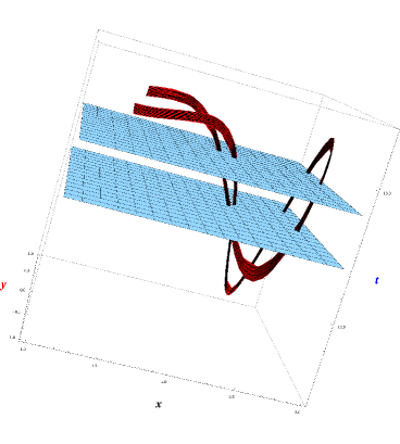
Figure 8: Region $3$ in Fig. 5, $n=3$ , $\gamma=4$ , $\tau^{\prime}\equiv(4,4.01)$, $\epsilon=0.1$, $\sigma^{\prime}\equiv(\pi,\frac{3\pi}{2})$.

Let us now write down the perturbations for $P_{1}$. We find

$$t^{\prime}=t+\phi n^{0}=t+\epsilon\rho_{0}\cos\gamma\omega\tau\sin\omega\sigma\cos\omega\sigma\,\,{}_{2}F_{1}(\frac{2+\gamma}{2},\frac{2-\gamma}{2},\frac{1}{2};\sin^{2}{\omega\sigma})\ ,$$ (50)

$$\rho^{\prime}=\rho+n^{1}\phi=\rho-\epsilon\rho_{0}\frac{\bar{a}\cos\gamma\omega\tau\cos^{2}\omega\sigma\,\,{}_{2}F_{1}(\frac{2+\gamma}{2},\frac{2-\gamma}{2},\frac{1}{2};\sin^{2}{\omega\sigma})}{\sqrt{{\bar{a}}^{2}+(1-{\bar{a}}^{2})\sin^{2}\omega\sigma}}\,$$ (51)

$$\theta^{\prime}=\theta+n^{2}\phi=\theta+\epsilon\rho_{0}\frac{\omega\cos\gamma\omega\tau\sin\omega\sigma\cos\omega\sigma\,\,{}_{2}F_{1}(\frac{2+\gamma}{2},\frac{2-\gamma}{2},\frac{1}{2};\sin^{2}{\omega\sigma})}{{\bar{a}}^{2}+(1-{\bar{a}}^{2})\sin^{2}\omega\sigma}$$ (52)

As before, defining $x^{\prime}=\rho^{\prime}\cos\theta^{\prime}$ and $y^{\prime}=\rho^{\prime}\sin\theta^{\prime}$ and with $\rho^{\prime}=\rho+\delta\rho$ and $\theta^{\prime}=\theta+\delta\theta$ we evaluate $\delta t$, $\frac{\delta\rho}{\rho}$ and $\delta\theta$ using the $(\tau^{\prime},\sigma^{\prime})$ coordinates to finally obtain $t^{\prime}$, $x^{\prime}$ and $y^{\prime}$ which are as follows

$$t^{\prime}=t+\frac{\epsilon\rho_{0}}{4}[\sin[\{(\frac{\gamma}{2}-1)n+2\}\tau^{\prime}+\{(\frac{\gamma}{2}-1)n-2\}\sigma^{\prime}]-\sin\{(\frac{\gamma}{2}+1)n-2\}(\tau^{\prime}+\sigma^{\prime})]$$

$${}_{2}F_{1}(\frac{2+\gamma}{2},\frac{2-\gamma}{2},\frac{1}{2};\sin^{2}\frac{(n-2)\tau^{\prime}+n\sigma^{\prime}}{2})\hskip 36.135pt$$ (53)

$$x^{\prime}=C(\tau^{\prime},\sigma^{\prime})\,\,x+D(\tau^{\prime},\sigma^{\prime})\,\,y$$ (54)

$$y^{\prime}=-D(\tau^{\prime},\sigma^{\prime})\,\,x+C(\tau^{\prime},\sigma^{\prime})\,\,y$$ (55)

where $C$ and $D$ are

$$C=1-\frac{\epsilon(n-2)^{2}\cos^{2}{\frac{n\sigma^{\prime}+(n-2)\tau^{\prime}}{2}}\cos{\frac{\gamma(n-2)\sigma^{\prime}+\gamma n\tau^{\prime}}{2}}{}_{2}F_{1}(\frac{2+\gamma}{2},\frac{2-\gamma}{2},\frac{1}{2};\sin^{2}{\frac{n\sigma^{\prime}+(n-2)\tau^{\prime}}{2}})}{(n-2)^{2}+4(n-1)\sin^{2}{\frac{n\sigma^{\prime}+(n-2)\tau^{\prime}}{2}}}\ ,$$ (56)

$$D=\frac{\epsilon n(n-2)\sin\left[n\sigma^{\prime}+(n-2)\tau^{\prime}\right]\cos{\frac{\gamma(n-2)\sigma^{\prime}+\gamma n\tau^{\prime}}{2}}\,{}_{2}F_{1}(\frac{2+\gamma}{2},\frac{2-\gamma}{2},\frac{1}{2};\sin^{2}{\frac{n\sigma^{\prime}+(n-2)\tau^{\prime}}{2}})}{2(n-2)^{2}+8(n-1)\sin^{2}{\frac{n\sigma^{\prime}+(n-2)\tau^{\prime}}{2}}}\ .$$ (57)

Figures 5 and 6 show the unperturbed and perturbed profiles for $n=3$ and $\gamma=4$. We can see that, as for $\gamma=2$, the spikes are rounded off, as is visible in the plot for a small range of $\sigma^{\prime}$ (corresponding to region $1$ in Figure 5), shown in Figure 6. In Figures 7 and 8 we plot the worldsheets over other different ranges of $\sigma^{\prime}$ (corresponding to the regions 2 and 3 in Figure 5) but for the same range of $\tau^{\prime}$.

3.3 Dual spiky strings and perturbations

In this section we discuss the T-dual solutions of the spiky strings first obtained in [31]. As before, we assume a $2+1$ dimensional flat background spacetime in $t,\rho,\theta$ coordinates. To arrive at the dual spikes we use the dual Jevicki-Jin embedding given by

$$t=\sigma+f(\tau),\>\>\>\rho=\rho(\tau),\>\>\>\theta=\omega\sigma+g(\tau)\ .$$ (58)

This embedding can be obtained from the original Jevicki-Jin embedding by exchanging the world sheet coordinates $\tau$ and $\sigma$. Later, we will see why it is necessary to have the dual embedding in order to obtain the dual spikes.

Using the above in the string equations of motion and constraints we can obtain the functions $\rho(\tau)$, $f(\tau)$ and $g(\tau)$. The string equations of motion and the Virasoro constraints are of the same form, with $\tau$ derivatives now replacing the $\sigma$ derivatives. Finally, we write the dual solution as,

$$t=\sigma+{\bar{a}}\tau,\>\>\>\rho=\frac{1}{\omega}\left[1+({\bar{a}}^{2}-1)\sin^{2}\omega\tau\right]^{\frac{1}{2}},\>\>\>\theta=\omega\sigma+\tan^{-1}\left[\bar{a}\tan\{\omega\tau\}\right]\ .$$

Here $\bar{a}=\frac{\rho_{0}}{\rho_{1}}>1$, whereas, for the spike solution, $\bar{a}<1$. The relation between $\rho_{0}$ and $\rho_{1}$ is

$$\frac{\rho_{0}-\rho_{1}}{\rho_{1}+\rho_{0}}=\frac{1}{n-1}\ ,$$ (60)

and

$$\bar{a}=\frac{n-2}{n},\hskip 14.45377pt\omega=\frac{1}{\rho_{1}}\ .$$ (61)

To write the dual spike solution in Cartesian coordinates we will need to use a coordinate transformation similar to the one mentioned earlier but with $\tau$ and $\sigma$ exchanged. Working through some straightforward algebra we arrive at

$$x=\frac{\rho_{0}}{n}\left[(n-1)\cos\left(\tau^{\prime}-\sigma^{\prime}\right)+\cos\{(n-1)\left(\tau^{\prime}+\sigma^{\prime}\right)\}\right]\,$$

$$y=\frac{\rho_{0}}{n}\left[(n-1)\sin\left(\tau^{\prime}-\sigma^{\prime}\right)-\sin\{(n-1)\left(\tau^{\prime}+\sigma^{\prime}\right)\}\right]\ .$$ (62)

It is important to realise that in the Jevicki-Jin conformal gauge the dual spiky string must be obtained using the dual embedding which has $\tau$ dependent functions (as opposed to $\sigma$ dependent functions in the spiky string case). The reason behind this fact may be traced to the correct signature of the induced metric, which is Lorentzian only when the dual embedding is used.

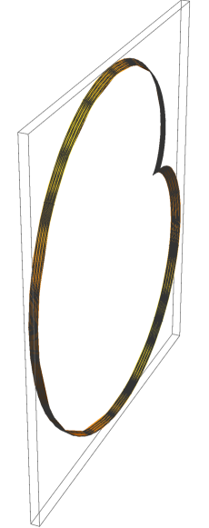
Figure 9: $n=3$, $\tau^{\prime}\equiv(4.0,4.03)$. Unperturbed.

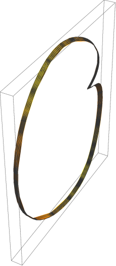
Figure 10: $n=3$, $\gamma=2$, $\epsilon=0.08$, $\tau^{\prime}\equiv(4.0,4.03)$. Perturbed.

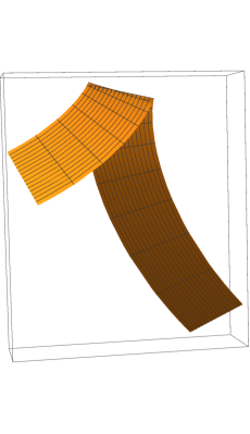
Figure 11: $n=3$, $\tau^{\prime}\equiv(4.0,4.03)$, unperturbed.

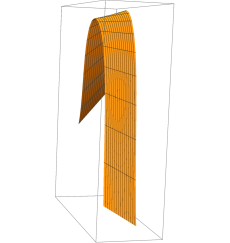
Figure 12: $n=3$, $\gamma=2$, $\epsilon=0.08$, $\tau^{\prime}\equiv(4.0,4.01)$, perturbed.

We now proceed to find the perturbation equations. We need to write down the tangent, normal, induced metric and extrinsic curvature for the world sheet. The tangent vector to the worldsheet is given as

$$e^{i}_{\tau}=\left(\dot{f},\dot{\rho},\dot{g}\right),\hskip 14.45377pte^{i}_{\sigma}=\left(1,0,\omega\right)\ .$$ (63)

Using the expressions for $f$, $g$ and $\rho$ quoted above the induced line element turns out to be:

$$ds^{2}=\left(\rho^{2}\omega^{2}-1\right)\left(-d\tau^{2}+d\sigma^{2}\right)\ .$$ (64)

The normal to the worldsheet is given as:

$$n^{i}=\left(\cot\omega\tau,-\frac{\bar{a}}{\omega\rho},\frac{\cot\omega\tau}{\omega\rho^{2}}\right)\ .$$ (65)

The extrinsic curvature tensor turns out to be

$$K_{ab}=\begin{pmatrix}\bar{a}\omega&\omega\cr\omega&\bar{a}\omega\end{pmatrix}\ .$$ (66)

Note that all entries in the above matrix are now positive. The quantity $K_{ab}K^{ab}$ is given as

$$K_{ab}K^{ab}=\frac{2\omega^{2}(\bar{a}^{2}-1)}{(\rho^{2}\omega^{2}-1)^{2}}=-{}^{2}R\ .$$ (67)

The Ricci scalar of the dual worldsheet is negative (in the spiky string case it was positive) and it diverges at the spike locations. Substituting the above stated quantities in the perturbation equation and separating $\tau$ and $\sigma$ dependent parts we get

$$\frac{d^{2}P}{d\zeta^{2}}+(\gamma^{2}-\frac{2}{\sin^{2}{\zeta}})P=0\ ,$$ (68)

where $\beta=\gamma\omega$ and $\zeta=\omega\tau$. A simple solution for $\gamma=2$ is $P(\zeta)=\sin^{2}{\zeta}$. We have the perturbation scalar as $\phi=\epsilon\rho_{0}\cos 2\omega\sigma\sin^{2}\omega\tau$. Following the same steps as for spiky strings, we get, for the dual spikes,

$$\delta t=\frac{\epsilon\rho_{0}}{4}\left[\sin 2(\tau^{\prime}-\sigma^{\prime})+\sin 2(n-1)(\tau^{\prime}+\sigma^{\prime})\right]\ ,$$ (69)

$$\frac{\delta\rho}{\rho}=\frac{\epsilon n^{2}\cos\left[(n-2)\tau^{\prime}+n\sigma^{\prime}\right]\sin^{2}\left[\frac{n}{2}\tau^{\prime}+\frac{n-2}{2}\sigma^{\prime}\right]}{(n-2)^{2}+4(n-1)\sin^{2}\left[\frac{n}{2}\tau^{\prime}+\frac{n-2}{2}\sigma^{\prime}\right]}\ ,$$ (70)

$$\delta\theta=\frac{\epsilon n(n-2)\cos\left[(n-2)\tau^{\prime}+n\sigma^{\prime}\right]\sin\left[\frac{n}{2}\tau^{\prime}+\frac{n-2}{2}\sigma^{\prime}\right]}{(n-2)^{2}+4(n-1)\sin^{2}\left[\frac{n}{2}\tau^{\prime}+\frac{n-2}{2}\sigma^{\prime}\right]}$$ (71)

Expressions for $t^{\prime}$, $x^{\prime}$ and $y^{\prime}$ can therefore be obtained, as done earlier for the spiky string case.

Figures 9 and 10 show the unperturbed and perturbed worldsheets over the entire range of $\sigma^{\prime}$. Figures 11 and 12 are for the unperturbed and perturbed worldsheets plotted over a restricted range of $\sigma^{\prime}$ in the neighborhood of the spike. The rounding off of the spike is clearly visible in Figures 10 and 12. In general, solving this equation for $P(\zeta)$ we find one oscillatory solution and one diverging solution. For the oscillatory solution we have

$$P(\zeta)=\epsilon\sin^{2}{\zeta}{}_{2}F_{1}(\frac{2+\gamma}{2},\frac{2-\gamma}{2},\frac{5}{2};\sin^{2}{\zeta})\ .$$ (72)

It is easy to obtain various cases for different $\gamma$ values and plot the perturbed string profile. We have shown here images for different values of $\gamma$ too. In Figure 13, we have shown the perturbed profile for $\gamma=4$ and in Figure 14 we have shown a closer look of the same profile in the neighborhood of the spike, by plotting, as before, for a restricted range of $\sigma^{\prime}$. Similarly, the $\gamma=6$ case is shown in Figure 15 and 16. In both these cases, we notice the rounding off of the spikes.

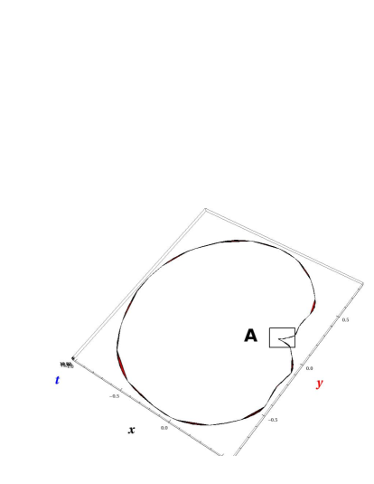
Figure 13: $n=3$, $\tau^{\prime}\equiv(4.0,4.0001)$, $\sigma^{\prime}\equiv(0,2\pi),\gamma=4$.

Figure 14: Region A in Figure 13, $n=3$, $\tau^{\prime}\equiv(4.0,4.0001)$, $\sigma^{\prime}\equiv(\pi,\frac{4\pi}{3}),\gamma=4$,

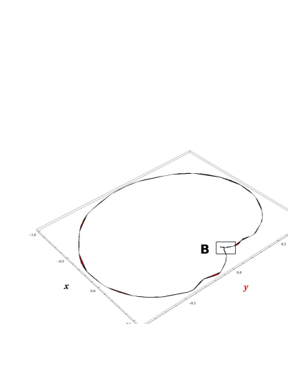
Figure 15: $n=3$, $\tau^{\prime}\equiv(4.0,4.0001)$, $\sigma^{\prime}\equiv(0,2\pi),\gamma=6$.

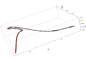
Figure 16: Region B in Figure 15, $n=3$, $\tau^{\prime}\equiv(4.0,4.0001)$, $\sigma^{\prime}\equiv(\pi,\frac{4\pi}{3}),\gamma=6$.

Thus, based on the above analysis, we can surely conclude that the effect of normal perturbations of the dual spiky string also appears through a resolution or rounding off, of the spikes. This is indeed an indicator that both the spiky string and its dual are stable classical solutions of the string equations of motion and the Virasoro constraints.

4 Extension to $3+1$ dimensions: solutions and perturbations

It is quite straightforward to generalise the above discussion to a $3+1$ dimensional background spacetime. We consider a flat $3+1$ dimensional background spacetime with a line element

$$ds^{2}=-dt^{2}+d\rho^{2}+\rho^{2}d\theta^{2}+\rho^{2}\sin^{2}{\theta}d\phi^{2}\ .$$ (73)

We choose the embedding as

$$t=\tau+f(\sigma),\hskip 14.45377pt\rho=\rho(\sigma),\hskip 14.45377pt\phi=\omega\tau+g(\sigma),\hskip 14.45377pt\theta=\frac{\pi}{2}\ .$$ (74)

Using the above, in the string equations of motion and constraints, we can show that the functions $\rho(\sigma)$, $f(\sigma)$ and $g(\sigma)$ take the forms mentioned earlier. The only novelty is the fact that we are confined to the equatorial plane, $\theta=\frac{\pi}{2}$.

Let us now convert this solution to Cartesian coordinates. This will enable us to plot the profiles of the unperturbed and perturbed string worldsheets. The Cartesian embedding functions $x$, $y$ and $z$ as functions of $\tau^{\prime}$ and $\sigma^{\prime}$ are given as

$$x = \frac{\rho_{0}}{n-2}\left[(n-1)\cos\left(\tau^{\prime}-\sigma^{\prime}\right)-\cos\{(n-1)\left(\tau^{\prime}+\sigma^{\prime}\right)\}\right]\ ,$$

$$y = \frac{\rho_{0}}{n-2}\left[(n-1)\sin\left(\tau^{\prime}-\sigma^{\prime}\right)-\sin\{(n-1)\left(\tau^{\prime}+\sigma^{\prime}\right)\}\right]\ .$$

$$z = 0\ .$$

To work out the perturbations we will proceed as the $2+1$ case. The tangent vectors to the worldsheet are,

$$e^{i}_{\tau}=\left(1,0,0,\omega\right),\hskip 14.45377pte^{i}_{\sigma}=\left(f^{\prime},\rho^{\prime},0,g^{\prime}\right)\ .$$ (76)

The induced metric is, as before.

$$ds^{2}=\left(1-\rho^{2}\omega^{2}\right)\left(-d\tau^{2}+d\sigma^{2}\right)\ .$$ (77)

The number of the normals on any embedded surface is given by $N-D$, where $N$ is the background spacetime dimension and $D$ is the dimension of the surface. In the $2+1$ case, there is only one normal but for the $3+1$ case there will be two normals. The normals to the worldsheet are chosen as

$$n^{i(1)}=\left(\tan\omega\sigma,-\frac{\bar{a}}{\omega\rho},0,\frac{\tan\omega\sigma}{\omega\rho^{2}}\right)\ .$$ (78)

$$n^{i(2)}=\left(0,0,\frac{1}{\rho},0\right)\ .$$ (79)

The two different extrinsic curvature tensors (along the two different normals) turn out to be

$$K_{ab}^{(1)}=\begin{pmatrix}-\bar{a}\omega&-\omega\cr-\omega&-\bar{a}\omega\ ,\end{pmatrix}$$ (80)

and

$$K_{ab}^{(2)}=0\ .$$ (81)

Hence the quantity $K_{ab}^{\alpha}K_{\beta}^{ab}$ is given as

$$K_{ab}^{\alpha}K_{\beta}^{ab}=-\frac{2\omega^{2}(1-\bar{a}^{2})}{(1-\rho^{2}\omega^{2})^{2}}\delta^{\alpha}_{\beta}\ .$$ (82)

Since the background is flat, the Riemann tensor is zero and therefore the equation for the perturbation scalar along $n^{i(1)}$ becomes:

$$\left(-\frac{\partial^{2}}{\partial\tau^{2}}+\frac{\partial^{2}}{\partial\sigma^{2}}\right)\phi^{(1)}-\frac{2\omega^{2}(1-\bar{a}^{2})}{(1-\rho^{2}\omega^{2})^{2}}\phi^{(1)}=0\ .$$ (83)

Using the functional form of $\rho(\sigma)$ one can reduce this equation to

$$\left(-\frac{\partial^{2}}{\partial\tau^{2}}+\frac{\partial^{2}}{\partial\sigma^{2}}\right)\phi^{(1)}-2\omega^{2}\sec^{2}\omega\sigma\phi^{(1)}=0\ .$$ (84)

Let us take a simple separable ansatz

$$\phi^{(1)}{(\sigma)}=e^{i\beta\tau}\chi(\sigma)\ .$$ (85)

Using a simple transformation $\xi=\omega\sigma$ the equation for $\chi(\sigma)$ reduces to that for the $P(\sigma)$ in the $2+1$ case. The equation for the perturbation scalar along the second normal turns out to be

$$\left(-\frac{\partial^{2}}{\partial\tau^{2}}+\frac{\partial^{2}}{\partial\sigma^{2}}\right)\phi^{(2)}=0\ .$$ (86)

The general solution of (86) is of the form

$$\phi^{(2)}(\sigma)=C_{1}g(\tau+\sigma)+C_{2}h(\tau-\sigma)\ .$$ (87)

The general solution for (84) is

$$\chi(\xi)=C_{1}\chi_{1}+C_{2}\chi_{2}\ ,$$ (88)

where $\chi_{1}$ and $\chi_{2}$ are $P_{1}$ and $P_{2}$ respectively, as described in the previous section in (47) and (48) and $\chi_{1}$ is the converging solution. If we choose $\gamma=2$ a solution is given as

$$\chi_{1}(\xi)=\epsilon\rho_{0}\cos^{2}{\xi}\ .$$ (89)

For the $\tau$ solution we take it’s real part(i.e. $\cos{\beta\tau}=\cos{2\omega\tau}$). For (87) we can consider a special case without loss of generality, as the following

$$\phi^{(2)}={\bar{\epsilon}}\rho_{0}\{\cos{\frac{(\tau+\sigma)\rho_{0}}{\rho_{1}}}+\cos{\frac{(\tau-\sigma)\rho_{0}}{\rho_{1}}}\}$$ (90)

where $\bar{\epsilon}\neq\epsilon$ is the amplitude of the perturbation. The perturbed embedding is given as

$$t^{\prime}=t+\phi^{(1)}n^{0}_{(1)}+\phi^{(2)}n^{0}_{(2)}=t+\epsilon\rho_{0}\cos\gamma\omega\tau\sin\omega\sigma\cos\omega\sigma\ ,$$ (91)

$$\rho^{\prime}=\rho+n^{1}_{(1)}\phi^{(1)}+n^{1}_{(2)}\phi^{(2)}=\rho-\epsilon\rho_{0}\frac{\bar{a}\cos\gamma\omega\tau\cos^{2}\omega\sigma}{\sqrt{{\bar{a}}^{2}+(1-{\bar{a}}^{2})\sin^{2}\omega\sigma}}\,$$ (92)

$$\theta^{\prime}=\theta+n^{2}_{(1)}\phi^{(1)}+n^{2}_{(2)}\phi^{(2)}=\frac{\pi}{2}+\frac{{\bar{\epsilon}}\rho_{0}}{\rho}\{\cos{\frac{(\tau+\sigma)\rho_{0}}{\rho_{1}}}+\cos{\frac{(\tau-\sigma)\rho_{0}}{\rho_{1}}}\}\ ,\hskip 14.45377pt$$ (93)

$$\phi^{\prime}=\phi+n^{3}_{(1)}\phi^{(1)}+n^{3}_{(2)}\phi^{(2)}=\phi+\epsilon\rho_{0}\frac{\omega\cos\gamma\omega\tau\sin\omega\sigma\cos\omega\sigma}{{\bar{a}}^{2}+(1-{\bar{a}}^{2})\sin^{2}\omega\sigma}\ .$$ (94)

We need to switch back to Cartesian coordinates to get a clearer picture here. Defining $x^{\prime}=\rho^{\prime}\sin{\theta^{\prime}}\cos{\phi^{\prime}}$, $y^{\prime}=\rho^{\prime}\sin{\theta^{\prime}}\sin{\phi^{\prime}}$ and $z^{\prime}=\rho^{\prime}\cos{\theta^{\prime}}$ and using $\rho^{\prime}=\rho+\delta\rho$, $\theta^{\prime}=\theta+\delta\theta$ and $\phi^{\prime}=\phi+\delta\phi$ this eventually yields

$$x^{\prime}=x+\frac{\delta\rho}{\rho}x-\delta\phi y,\>\>\>y^{\prime}=y+\frac{\delta\rho}{\rho}y+\delta\phi x,\>\>\>z^{\prime}=-\rho\delta\theta\ .$$

Using the worldsheet coordinate transformation (13) and the relation (15) we can write the perturbed solution in Cartesian coordinates, for $\tau^{\prime}=0$ as follows,

$$x^{\prime}=x(1-\frac{\epsilon(n-2)^{2}\cos^{2}{\frac{n\sigma^{\prime}}{2}}\cos{(n-2)\sigma^{\prime}}}{(n-2)^{2}+4(n-1)\sin^{2}{\frac{n\sigma^{\prime}}{2}}})+y\frac{\epsilon n(n-2)\sin{\frac{n\sigma^{\prime}}{2}}\cos{\frac{n\sigma^{\prime}}{2}}\cos{(n-2)\sigma^{\prime}}}{(n-2)^{2}+4(n-1)\sin^{2}{\frac{n\sigma^{\prime}}{2}}}\ ,$$ (96)

Figure 17: Top view w.r.t. $z=0$ plane.

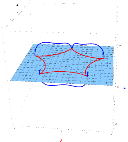
Figure 18: View from below $z=0$ plane.

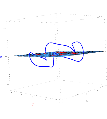
Figure 19: Side view.

$$y^{\prime}=-x\frac{\epsilon n(n-2)\sin{\frac{n\sigma^{\prime}}{2}}\cos{\frac{n\sigma^{\prime}}{2}}\cos{(n-2)\sigma^{\prime}}}{(n-2)^{2}+4(n-1)\sin^{2}{\frac{n\sigma^{\prime}}{2}}}+y(1-\frac{\epsilon(n-2)^{2}\cos^{2}{\frac{n\sigma^{\prime}}{2}}\cos{(n-2)\sigma^{\prime}}}{(n-2)^{2}+4(n-1)\sin^{2}{\frac{n\sigma^{\prime}}{2}}})\ ,\hskip 14.45377pt$$ (97)

$$z^{\prime}=-{\epsilon^{\prime}}\{\cos{(n-1)\sigma^{\prime}}+\cos{\sigma^{\prime}}\}\ .$$ (98)

Here $\epsilon^{\prime}={\bar{\epsilon}}\rho_{0}$. In Figures 19, 19 and 19 we have shown the perturbed (blue) and unperturbed (red) string profiles together assuming $\epsilon=\bar{\epsilon}$. The red curve is lying on the $z=0$ plane whereas the black curve is the perturbed profile. In the perturbed profile we can see that the spikes have been rounded off and the string is oriented in three dimensions (not exclusively on the $z=0$ plane). Figures 19 and 19 show how the perturbed string would look like from the upper ($z>0$) and lower ($z<0$) regions of the $z$-axis. Figure 19 combines these two pictures and demonstrates how the string is now no longer confined in the $z=0$ plane. The feature shown in Figures 19,19 and 19 demonstrate how the spikes disappear and smooth out because of the presence of the extra dimension ($z$ coordinate). We have verified this for other values of $\tau$ and also for the dual spiky string. It is to be noted that for the simple case of $\epsilon=0$ and $\bar{\epsilon}\neq 0$ we have $z^{\prime}$ different from $z=0$ whereas the $x^{\prime}=x$ and $y^{\prime}=y$. Here too the perturbed profile spreads into the $z$ direction leading to the spikes disappearing. One may also consider the full worldsheet by taking into account the $t$ (or $t^{\prime}$) direction as well. Such a scenario, of course, cannot be visualised or plotted. But the result about rounding off of the spikes remains unaltered.

5 Conclusions

In this paper, we have first shown that the simplest spiky strings in a $2+1$ dimensional flat background are stable against normal perturbations. The stability is demonstrated through the rounding off of the spikes when the string is slightly perturbed. We have shown this explicitly by solving the perturbation equations and obtaining the perturbed string configurations. The rounding off of the spikes (for nonzero angular momentum or winding), at the level of classical solutions, have been noticed earlier while studying spiky strings and their duals in $AdS_{3}\times S^{1}$ with energy (E), spin (S) in $AdS_{3}$ and angular momentum (J), winding (m) in $S^{1}$ [19][31].

In our analysis here which, of course, is for spiky strings and their duals in a flat background, it is the worldsheet perturbations which do the job of rounding off of the spikes. The perturbations are stable for particular values of the parameter $\gamma$ and also for a choice, among linearly independent solutions (the $P_{1}$ solution mentioned above). Further, we have seen that the perturbation equation turns out to be a special case of the time independent Schrodinger equation of a particle in a Poschl Teller potential. Our illustrations here are restricted to some simple exact solutions of the perturbation equations (specific values of the parameter $\gamma$) though, using the general solution one can surely find out the nature of the perturbation for any allowed mode (i.e. any $\gamma$).

We have also studied the dual spike solutions. In the dual spiky string case we have first introduced a dual emdedding in the conformal gauge (Jevicki-Jin gauge) to write down the string configurations. Thereafter, following the same procedure as for the spiky string case, we have obtained the perturbation equation and its solutions. Here too, the rounding off of the spikes is visible in the worldsheet profiles. It is worth noting here that the perturbation equation for perturbation scalar, for the dual spikes, is also a special case (but different from that for the spiky string) of the Poschl Teller potential problem in quantum mechanics. It may thus be worth addressing an inverse problem–does there exist a string configuration for which the perturbation equation will involve the full Poschl-Teller potential (i.e. a combination of the two special cases we have found here).

The spiky strings in $2+1$ dimensions can easily be extended to a $3+1$ dimensional background flat spacetime. Here we have also worked out the normal perturbations and obtain the perturbed worldsheet. We find that the presence of the additional dimension in the background leads to a rounding off of the spikes. Further, if we consider the full worldsheet evolution the rounding off persists. Therefore, one may argue that in a $3+1$ dimensional flat spacetime too the spiky solutions are indeed stable.

An obvious extension of this work is to investigate the perturbations of the AdS spiky strings which are relevant in the context of the AdS-CFT correspondence. In particular, it will be useful to know how the perturbations are related to the operators in the dual field theory side of the correspondence. We hope to communicate our results on normal perturbations of the spiky strings in AdS spacetime and also discuss possible connections with the associated field theory, in the near future.

References

- [1] C. J. Burden and L. J. Tassie, “Some exotic mesons and glueballs from the string model,” Phys. Letts. B 110, 64 (1982).
- [2] C. J. Burden and L. J. Tassie, “Rotating strings, glueballs and exotic mesons,” Aust. Jr. Phys. 35, 223 (1982).
- [3] C. J. Burden and L. J. Tassie, “ Additional rigidly rotating solutions in the string model of hadrons,” Aust. Jr. Phys. 37, 1 (1984).
- [4] C. J. Burden, “Gravitational radiation from a particular class of cosmic strings,” Phys. Letts. B, 164, 277 (1985).
- [5] F. Embacher, “Rigidly rotating cosmic strings,” Phys. Rev. D 46, 3659 (1992); Erratum Phys. Rev. D 47, 4803 (1993).
- [6] H. de Vega and I. L. Egusquiza, “ Planetoid string solutions in axisymmetric spacetimes”, Phys. Rev. D 54, 7513 (1996).
- [7] V. Frolov, S. Hendy and J. P. de Villiers, “ Rigidly rotatingstrings in stationary axisymmetric spacetime”, Class. Qtm. Grav. 14, 1099 (1997).
- [8] S. Kar and S. Mahapatra, “ Planetoid strings: solutions and perturbations”, Class. Qtm. Grav. 15, 1421 (1998).
- [9] C. J. Burden, “Comment on “Stationary rotating strings as relativistic particle mechanics”,” Phys. Rev. D 78, 128301 (2008).
- [10] K. Ogawa, H. Ishihara, H. Kozaki, H. Nakano and S. Saito, “ Stationary rotating strings as relativistic particle mechanics ”, Phys. Rev. D 78, 023525 (2008).
- [11] J. M. Maldacena, “The Large N limit of superconformal field theories and supergravity,” Int. J. Theor. Phys. 38, 1113 (1999) [Adv. Theor. Math. Phys. 2, 231 (1998)] [hep-th/9711200].
- [12] M. Kruczenski, “Spiky strings and single trace operators in gauge theories,” JHEP 0508, 014 (2005) [arXiv:hep-th/0410226].
- [13] S. S. Gubser, I. R. Klebanov and A. M. Polyakov, Nucl. Phys. B 636, 99 (2002) [hep-th/0204051].
- [14] G. Mandal, N. V. Suryanarayana and S. R. Wadia, “Aspects of semiclassical strings in AdS(5),” Phys. Lett. B 543, 81 (2002) [hep-th/0206103].
- [15] I. Bena, J. Polchinski and R. Roiban, “Hidden symmetries of the AdS(5) x S**5 superstring,” Phys. Rev. D 69, 046002 (2004) [hep-th/0305116].
- [16] J. A. Minahan and K. Zarembo, “The Bethe ansatz for N=4 superYang-Mills,” JHEP 0303, 013 (2003) [hep-th/0212208].
- [17] S. Frolov and A. A. Tseytlin, “Multispin string solutions in AdS(5) x S**5,” Nucl. Phys. B 668, 77 (2003) [hep-th/0304255].
- [18] R. Ishizeki and M. Kruczenski, “Single spike solutions for strings on and ,” Phys. Rev. D 76, 126006 (2007) [arXiv:0705.2429 [hep-th]].
- [19] R. Ishizeki, M. Kruczenski, A. Tirziu and A. A. Tseytlin, “Spiky strings in and their AdS-pp-wave limits,” Phys. Rev. D 79, 026006 (2009) [arXiv:0812.2431 [hep-th]].
- [20] S. Biswas and K. L. Panigrahi, “Spiky Strings on I-brane,” JHEP 1208, 044 (2012) [arXiv:1206.2539 [hep-th]].
- [21] A. Banerjee, K. L. Panigrahi and P. M. Pradhan, “Spiky strings on with NS-NS flux,” Phys. Rev. D 90, no. 10, 106006 (2014) [arXiv:1405.5497 [hep-th]].
- [22] A. Banerjee, S. Bhattacharya and K. L. Panigrahi, “Spiky strings in -deformed ,” JHEP 1506, 057 (2015) [arXiv:1503.07447 [hep-th]].
- [23] S. Frolov and A. A. Tseytlin, “Semiclassical quantization of rotating superstring in AdS(5) x S**5,” JHEP 0206, 007 (2002) [hep-th/0204226].
- [24] J. Garriga and A. Vilenkin, “Black holes from nucleating strings,” Phys. Rev. D 47 3265 (1993).
- [25] J. Guven, “Perturbations of a topological defect as a theory of coupled scalar fields in curved space interacting with an external vector potential,” Phys. Rev. D 48, 5562 (1993).
- [26] V. Frolov and A. L. Larsen, “Propagation of perturbations along strings”, Nucl. Phys. B 414, 129 (1994).
- [27] R. Capovilla and J. Guven, “Geometry of deformations of relativistic membranes,” Phys. Rev. D 51, 6736 (1995).
- [28] V. Forini, V. Giangreco, M. Puletti, L. Griguolo, D. Seminara, E. Vescovi, “Remarks on the geometrical properties of semiclassically quantized strings”, J. Phys A: Math. Theor., 48, 475401 (2015)
- [29] A. Jevicki and K. Jin, “Solitons and AdS string solutions”, Int. Jr. Mod. Phys. A 23, 2289 (2008).
- [30] S. Flugge, “ Practical Quantum Mechanics”, Springer-Verlag, Berlin-Heidelberg (1971), see Pgs. 89-93.
- [31] A. E. Mosaffa, B. Safarzadeh, “Dual Spikes: New Spiky String Solutions” , JHEP 0708, 017 (2007).