Viscous energy dissipation in slender channels with porous or semipermeable walls

Abstract

We study the viscous dissipation in pipe flows in long channels with porous or semipermeable walls, taking into account both the dissipation in the bulk of the channel and in the pores. We give simple closed form expressions for the dissipation in terms of the axially varying flow rate $Q(x)$ and the pressure $p(x)$, generalizing the well known expression $\dot{W}=Q\,\Delta p$ for the case of impenetrable walls with constant $Q$ and a pressure difference $\Delta p$ between the ends of the pipe. When the pressure $p_{0}$ outside the pipe is constant, the result is the straightforward generalization $\dot{W}=\Delta\left[(p-p_{0})\,Q\right]$. Finally, applications to osmotic flows are considered.

I Introduction

Channel flows – liquid flows confined within a closed conduit with no free surfaces – are omnipresent. In animals (LaBarbera, 1990) and plants (Holbrook and Zwieniecki, 2005) they serve as the building blocks of vascular systems, distributing energy to where it is needed and allowing distal parts of the organism to communicate. When constructed by humans, one of the major functions of channels is to transport liquids or gasses, e.g. water (irrigation and urban water systems) and energy (oil or natural gas) from sites of production to the consumer or industry.

In some cases, the channels have solid walls which are impermeable to the liquid flowing inside. In other cases, the channels have porous walls which allow the liquid to move across the wall and thus modify the axial flow. If solutes are present in the liquid, the walls can be semipermeable, allowing only the solvent to pass and thereby allow filtration or create osmotically driven flows due to concentration differences between the inside and the outside. Flows with impermeable walls have been studied in great detail, and analytical solutions are known in a few, but important, cases (Batchelor, 2000). Flows with porous walls have received much less attention, although they are equally important. The effect of porous walls is especially important in the study of biological flows (Holbrook and Zwieniecki, 2005; Marbach and Bocquet, 2016; Jensen et al., 2016) and in industrial filtration applications (Nielsen, 2012).

Exact solutions for the flow in porous walled channels are known in a few important cases. Berman’s method Berman (1953) allows for the solution of steady flows in geometries with symmetries, for example, between parallel plates or in a cylindrical tube. The technique is closely related to those commonly used in boundary layer theory (Schlichting and Gersten, 2000). By demanding that the solution be of similarity form, Berman’s method reduces the Navier-Stokes to a single non-linear third-order differential equation for the velocity potential in one space dimension. The flow between parallel plates (Berman, 1953) and in a cylindrical (Yuan and Finkelstein, 1956; Aldis, 1988) and annular tube (Berman, 1958) have been analyzed in this way. Time dependent flows, high-Reynolds-number flows, and stability and uniqueness of the solutions have since been address by a large number of workers using analytical and numerical methods, see e.g. Cox (1991); King and Cox (2001); Majdalani and Zhou (2003); Dauenhauer and Majdalani (2003); Kurdyumov (2008); Saad and Majdalani (2009); Xu et al. (2010); Liu and Prosperetti (2011).

Despite our broad knowledge of transport characteristics in porous channel flows, the energetic cost of flow remains poorly understood. In conventional low-Reynolds-number pipe flows, the link between the flow rate $Q$, pressure drop $\Delta p$ and energy dissipation rate is $\dot{W}=Q\Delta p$, analogous to an electrical circuit. However, in porous channels, both the flow rate and pressure are position-dependent, hence the standard result is inadequate.

In this paper we shall concentrate on the case of a long cylindrical pipe or tube with porous or semipermeable walls. We first (Section II) discuss the basic fluid dynamics based on the solution by Aldis Aldis (1988) for a long cylindrical porous pipe. In Section III, we write down the general expression for the viscous dissipation both in the bulk of the pipe and in its porous walls. Finally, in the last section, we discuss two specific examples, one where the porous inflow is constant, and and one where the external conditions are constant.

II Low-Reynolds-number flow in a long cylindrical, porous pipe

We consider a tube of length $L$ and characteristic transverse dimension $r_{0}$ embedded in a fluid-saturated medium (Fig. 1). The channel walls of thickness $d$ are permeable, characterized by the Darcy permeability $k$, such that the trans-membrane velocity field is normal to the channel walls

$${\mathbf{v}}_{m} =-\frac{k}{\eta d}\left(p_{e}(x)-p(x)\right){\hat{\mathbf{n}}}$$

$$=-L_{p}\left(p_{e}(x)-p(x)\right){\hat{\mathbf{n}}}=L_{p}\,\delta p(x)\,{\hat{\mathbf{n}}}$$ (1)

where $p_{e}$ and $p(x)$ is the external medium and channel pressure, respectively, $\delta p=p-p_{e}$ is the pressure drop across the membrane, and ${\hat{\mathbf{n}}}$ is the outward normal (i.e., $\hat{{\mathbf{r}}}$ in cylindrical coordinates) Further, $L_{p}=k/(\eta d)$ is the membrane permeability. A detailed model of $L_{p}$, assuming parallel cylindrical pores, is given in Appendix A.

When we are dealing semipermeable membranes separating solutions with different solute concentration, (1) takes the form

$${\mathbf{v}}_{m}=-L_{p}\left(\Psi_{e}(x)-\Psi(x)\right)\mathbf{n}=L_{p}\,\delta\Psi(x)$$ (2)

where $\Psi$ is the water potential. The water potential (free energy) $\Psi=p-\Pi$ includes the osmotic pressure $\Pi$, which, for low solute concentrations $c$, can be expressed using the van’t Hoff relation $\Pi=RTc$ (see e.g,. Fermi (1956)). Again, $\delta$ denotes the jump accross the membrane: $\delta\Psi=\Psi(x)-\Psi_{e}(x)$. In the rest of the paper, we assume separation of geometric scales, such that the channel is long in comparison to all other lengths, i.e., $L\gg r_{0}\gg d\gg\sqrt{k}$.

In steady low-Reynolds-number flow conditions, we base our analysis on the Stokes equation

$$\nabla p=\eta\nabla^{2}{\bf v},$$ (3)

for an incompressible fluid where $\nabla\cdot{\bf v}=0$ and a constant viscosity $\eta$ and density $\rho$. Note that the no-slip conditions on the channel boundaries correspond to $\mathbf{v}_{\perp}=\mathbf{v}_{m}$ and $\mathbf{v}_{\parallel}=\mathbf{0}$.

We express the velocity using axial and radial coordinates, i.e., $\mathbf{v}=(v_{x},v_{r})$ and thus assume rotational symmetry. In plants, the sieve tubes of the phloem are roughly of this form, and in the leaves their radii ($r_{0}$) are in the $\mu$m regime while their length ($L$) is centimetric. The slender (lubrication) approximation used by Aldis (1988) to describe such flows is valid, since $Re\ll 1$ and $r_{0}/L\ll 1$. The stationary flow field then has the form

$$v_{r}(r,x) =f(r)v_{0}(x)$$ (4)

$$v_{x}(r,x) =g(r)u(x)$$ (5)

where

$$f(r) =\frac{r^{3}}{r_{0}^{3}}-2\frac{r}{r_{0}}$$ (6)

$$g(r) =2\left(1-\frac{r^{2}}{r_{0}^{2}}\right)$$ (7)

The function $v_{0}(x)$ is the radial injection velocity

$$v_{r}(r_{0},x)=-v_{0}(x)=v_{m}(x)$$ (8)

where $v_{m}$ given by (1) or (2) such that a positive $v_{0}$ denotes an inflow. The mean axial flow speed is

$$u(x)=\frac{2\pi}{\pi r_{0}^{2}}\int_{0}^{r_{0}}v_{x}(r,x)\,r\mathrm{d}r={\bar{v}_{x}(r,x)}$$ (9)

and the corresponding volumetric flow rate $Q$ is

$$Q(x)=\pi r_{0}^{2}u(x)=Q_{0}+2\pi r_{0}\int_{0}^{x}v_{0}(x^{\prime})dx^{\prime}$$ (10)

where $Q_{0}$ is the inlet flow rate at $x=0$. The average flow speed is

$$u(x)=\frac{Q_{0}}{\pi r_{0}^{2}}+\frac{2}{r_{0}}\int_{0}^{x}v_{0}(x^{\prime})dx^{\prime}$$ (11)

or

$$u^{\prime}(x)=\frac{2}{r_{0}}v_{0}(x)$$ (12)

and

$$Q^{\prime}(x)=2\pi r_{0}v_{0}(x).$$ (13)

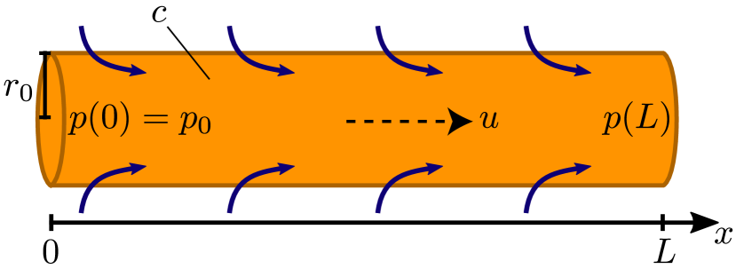
Figure 1: A tube of length $L$ and circular cross-section of radius $r_{0}$, is filled with a liquid of viscosity $\eta$ and density $\rho$. Liquid is injected from the surrounding medium (arrows) and creates a bulk flow of speed $u$ along the positive $x$-direction of the tube.

In the lubrication approximation the pressure does not vary over the pipe cross-section, i.e. we can replace $p$ by it’s average value $p(x)={\bar{p}(r,x)}$. Thereby the average velocity is related to the axial pressure gradient as in standard Hagen-Poiseuille flow

$$\frac{dp}{dx}=-\frac{8\eta}{r_{0}^{2}}u(x)=-\frac{8\eta}{\pi r_{0}^{4}}Q(x)$$ (14)

and, finally, the inflow $v_{0}(x)=-v_{m}$ is given by (1) or (2) depending on whether the membrane is fully permeably or only permeable to the solvent.

III Viscous dissipation

We shall determine the viscous dissipation in the flows studied in Section II, by looking firstly at the dissipation in the bulk flow, and secondly at the flow through the porous semipermeable walls, and then putting them together. Finally, we shall verify these expressions, by looking at the energy advection equation. The dissipated energy is given as (see e.g., Landau and Lifshitz (1987))

$$\dot{W}=\frac{1}{2}\eta\int\sum_{i,j}u_{ij}^{2}dV=\frac{1}{2}\eta\int Tr\left[{\rm\bf{u}}\cdot{\rm\bf{u}}^{T}\right]dV$$ (15)

where $u_{ij}$ is the strain rate

$$u_{ij}=\left(\frac{\partial v_{i}}{\partial x_{j}}+\frac{\partial v_{j}}{\partial x_{i}}\right)$$ (16)

and where the volume integral goes over the volume of the flow. The sum in (15), being the trace of the product of u-matrices, is invariant with respect to transformations to other (locally) orthogonal coordinates, and in particular, $i$ and $j$ can represent the cylindrical coordinates used above.

Note that this dissipative energy only represents the work done by the viscous forces in the fluid. For osmotically driven flows in plant leaves there would be an energy consumption related to the transport of sugar into the tubes, which we are not trying to account for here.

The dissipation has the form

$$\dot{W}_{\text{tot}}=\dot{W}_{\text{bulk}}+\dot{W}_{\text{walls}}$$ (17)

with terms coming coming from the bulk flow and from the flow in the porous walls.

The viscous dissipation for an axially symmetric flow, such as the Aldis flow field given by Eq. (4)-(5), can then be written as

$$\dot{W} =2\eta\int dV\left[\left(\frac{\partial v_{r}}{\partial r}\right)^{2}+\left(\frac{v_{r}}{r}\right)^{2}\right.$$

$$+\left.\left(\frac{\partial v_{x}}{\partial x}\right)^{2}+\frac{1}{2}\left(\frac{\partial v_{r}}{\partial x}+\frac{\partial v_{x}}{\partial r}\right)^{2}\right].$$ (18)

For the Aldis flow we can write the velocity components explicitly using (4)-(13). To obtain this solution, we made the assumption that $v_{r}\ll v_{x}$ and $\partial/\partial x\ll\partial/\partial r$, so the dominant term in the dissipation is

$$\dot{W}_{\text{bulk}}=\eta\int dV\left(\frac{\partial v_{x}}{\partial r}\right)^{2} =\eta\int dV\left(g^{\prime}(r)\right)^{2}u^{2}(x)$$

$$=\frac{8\eta}{\pi r_{0}^{4}}\int_{0}^{L}Q^{2}(x)dx$$ (19)

where we have used that $g^{\prime}(r)=-4r/r_{0}^{2}$ (7). Using the Hagen-Poiseuille relation (14) this can be written

$$\dot{W}_{\text{bulk}} =-\int_{0}^{L}p^{\prime}(x)Q(x)dx$$ (20)

and for a normal Poiseuille flow in a cylindrical pipe with solid walls (and therefore $Q$ and $p^{\prime}=\Delta p/L$ constant) this becomes $\dot{W}_{\text{bulk}}=Q\Delta p$ as it should. The additional terms in (18) can be written in descending orders of $\left(L/r_{0}\right)^{2}$ as

$$\Delta\dot{W}_{\text{add}}=$$

$$\frac{1}{3\pi}\frac{\eta}{r_{0}^{2}}\left[5\int_{0}^{L}\left(Q^{\prime}\right)^{2}dx+8\left(Q^{\prime}(L)Q(L)-Q^{\prime}(0)Q(0)\right)\right]$$

$$+\frac{11}{48\pi}\eta\int_{0}^{L}\left(Q^{\prime\prime}\right)^{2}dx$$ (21)

and in order of magnitude they correspond to replacing 2 or 4 factors of $r_{0}$ by factors of $L$ and it would thus not be justified to keep them in the lubrication limit used to obtain Eq. (4)-(5).

To discribe the dissipation in the porous tube wall, we use Darcy’s law (1) or (2) in the form

$$v_{0}(x) =\frac{k}{\eta d}\delta p=L_{p}\delta p$$ (22)

where $\delta p$ is the pressure jump across the porous tube wall, which, in osmotic flows, should be replaced by the jump in water potential $\delta\Psi=p-RTc$. The corresponding energy dissipation pr. unit wall area is simply $\dot{w}_{\text{mem}}=v_{0}\Delta p=(v_{0}(x))^{2}/L_{p}$ and the total dissipation is

$$\dot{W}_{\text{wall}}=2\pi r_{0}\int_{0}^{L}v_{0}(x)\,\delta p\,dx=\frac{2\pi r_{0}}{L_{p}}\int_{0}^{L}(v_{0}(x))^{2}dx$$

$$=\frac{1}{2\pi r_{0}L_{p}}\int_{0}^{L}(Q^{\prime}(x))^{2}dx=\int_{0}^{L}\delta p(x)\,Q^{\prime}(x)dx$$ (23)

The total dissipation is found by adding the wall contribution (23) to the bulk contribution (19) giving

$$\dot{W}_{\text{tot}} =-\int_{0}^{L}\left(p^{\prime}(x)\,Q(x)+\delta p(x)\,Q^{\prime}(x)\right)dx$$ (24)

which can also be written

$$\dot{W}_{\text{tot}} =\frac{8\eta}{\pi r_{0}^{4}}\left(\int_{0}^{L}\left(Q^{2}(x)+L^{2}_{0}\left(Q^{\prime}(x)\right)^{2}\right)\right)$$ (25)

where $L_{0}$ is the “efficient length” introduced by Rademaker et al. in the context of osmotically driven pipe flows Rademaker et al. (2017), and, earlier, by Landsberg and Fowkes in the context of water motion through root hairs Landsberg and Fowkes (1978).

$$L_{0}=\left(\frac{r_{0}^{3}}{16\eta L_{p}}\right)^{1/2}=\left(\frac{r_{0}^{3}d}{16k}\right)^{1/2}$$ (26)

If we go back to the variables $p$ (or $\Psi$) and $Q$, we can write these expressions in a more general way. In order to treat the porous and the semipermeable case together, we shall write the inflow condition (1)-(2) in general as

$$v_{0}(x)=-L_{p}\,\delta\Psi(x)$$ (27)

where we, in the porous case simply assume that $c=0$. Then, using (13) and (14), we get

$$\dot{W}_{\text{tot}} =-\int_{0}^{L}\left(p^{\prime}(x)\,Q(x)+\delta\Psi(x)\,Q^{\prime}(x)\right)dx$$ (28)

an expression which, like (24), is completely free of material parameters.

IV Special cases

IV.1 Constant inflow

If we assume a constant inflow $v_{0}$, we have $Q(x)=Q_{0}+2\pi r_{0}v_{0}x$ and

$$\dot{W}_{\text{tot}}=\frac{8\eta}{\pi r_{0}^{4}}\left(\int_{0}^{L}\left(Q^{2}(x)+L^{2}_{0}\left(Q^{\prime}(x)\right)^{2}\right)\right)$$

$$=32\pi\frac{\eta v_{0}^{2}L_{0}^{3}}{r_{0}^{2}}\left(\left((1+b^{2})m+bm^{2}+\frac{1}{3}m^{3}\right)\right)$$ (29)

where $m=L/L_{0}$ and $b=Q_{0}/(2\pi r_{0}v_{0}L_{0})$ are dimensionless numbers. For a tube closed in one end (like a pine needle) $Q_{0}=b=0$ and one can see that the membrane dissipation dominates for small $L\ll L_{0}$ and the bulk dissipation dominates for large $L\gg L_{0}$.

IV.2 Constant external conditions

If the pressure outside the tube $p_{e}$ is constant we can introduce the new pressure $p\to p-p_{e}$ in (24)) and get simply

$$\dot{W}_{\text{tot}}=\Delta[p\,Q]=p(0)Q(0)-p(L)Q(L)$$ (30)

generalizing the Hagen-Poiseuille result $\dot{W}=Q\,\Delta p$.

Similarly, for the osmotic case, if both the pressure and concentration outside the tube $c_{e}$ are constant, we can introduce the relative concentration $c\to c-c_{e}$ and similarly $\Psi\to\Psi-\Psi_{e}$ to get (using (28)

$$\dot{W}_{\text{tot}}=-\int_{0}^{L}(p^{\prime}(x)\,Q(x)+\Psi(x)\,Q^{\prime}(x))dx$$

$$=\int_{0}^{L}\left(\left(RTc(x)-p(x)\right)Q^{\prime}(x)-Q(x)p^{\prime}(x)\right)dx$$

$$=\int_{0}^{L}RTc(x)Q^{\prime}(x)dx-\int_{0}^{L}\frac{d}{dx}(pQ)dx$$

$$=\int_{0}^{L}RTc(x)Q^{\prime}(x)dx+\Delta[p\,Q]$$

$$=\Delta[\Psi\,Q]-\int_{0}^{L}RTc^{\prime}(x)Q(x)dx.$$ (31)

where $\Delta[\Psi\,Q)]=\Psi(0)Q(0)-\Psi(L)Q(L)$ and where we recover (30) for $c=0$.

If the concentration inside the tube is also constant, the dissipation for the osmotically driven flow is

$$\dot{W}_{\text{tot}} =\Delta[\Psi Q]$$ (32)

and if $Q$ is zero at $x=0$, the analytical solution Rademaker et al. (2017)

$$Q(x)= \frac{2\pi r_{0}L_{p}L}{m}\,(RTc-p(L))\frac{\sinh\left(m\frac{x}{L}\right)}{\cosh m}$$ (33)

$$RTc- p(0)=\frac{RTc-p(L)}{\cosh m}.$$ (34)

gives the simple form for the dissipation

$$\dot{W}_{\text{tot}} =-\Psi(L)Q(L)=\left(RTc-p(L)\right)Q(L)$$

$$=2\pi r_{0}LL_{p}(RTc-p(L))^{2}\frac{\tanh m}{m}.$$ (35)

The individual contributions are similarly

$$\dot{W}_{\text{lub}}=$$

$$\pi r_{0}LL_{p}(RTc-p(L))^{2}\left(-\frac{1}{\cosh^{2}m}+\frac{\tanh m}{m}\right)$$ (36)

and

$$\dot{W}_{\text{mem}}=$$

$$\pi r_{0}LL_{p}(RTc-p(L))^{2}\left(\frac{1}{\cosh^{2}m}+\frac{\tanh m}{m}\right)$$ (37)

so when we add these contributions the $1/\cosh^{2}m$ terms cancel. For small $m$, $\dot{W}_{\text{lub}}$ is very small ($O(m^{2})$)

$$\dot{W}_{\text{lub}}\approx\frac{1}{6}m^{2}\pi r_{0}LL_{p}(RTc-p(L))^{2}$$ (38)

whereas

$$\dot{W}_{\text{mem}}\approx\left(2-\frac{5}{6}m^{2}\right)\pi r_{0}LL_{p}(RTc-p(L))^{2}$$ (39)

so $\dot{W}_{\text{mem}}$ dominates completely. At large $m$ they become equal:

$$\dot{W}_{\text{lub}}\approx\dot{W}_{\text{mem}} \approx\frac{1}{m}\pi r_{0}LL_{p}(RTc-p(L))^{2}$$

$$=\pi r_{0}L_{\text{eff}}L_{p}(RTc-p(L))^{2}$$ (40)

although $\dot{W}_{\text{mem}}>\dot{W}_{\text{lub}}$ for all $m$.

The case $c=0$ corresponds to a porous pipe in a constant external pressure $p_{e}$. Again, if the pipe is closed at $x=0$ and open at $x=L$ with pressure $p(L)<p_{e}$, we get the exact same results, replacing $RTc-p(L)$ by $p_{e}-p(L)$ in (35), (36) and (37).

V Conclusions

We have studied the viscous energy dissipation in pipe flows with permeable or semipermeable walls in order to generalise the result $\dot{W}=Q\,\Delta p$ valid for pipes with impermeable walls. We have obtained a surprisingly simple expression valid for Stokes flow in long, thin, cylindrical pipe using the slender approximation and representing the porous wall as a collection of cylindrical pores. For a pipe of length $L$, the dissipation given in eqn. (25) is expressed in terms of the axially varying flow rate and its derivative as well as the material parameters: pipe radius, wall-permeability and liquid viscosity. For semipermeable pipes, where the water uptake is governed by osmosis, the viscous dissipation, given in eqn. (31), is expressed entirely in terms of the fundamental variables: the flux, the pressure and the osmotic pressure (or concentration) without any material parameters. This suggests that the result it is much more general than our derivation in terms of cylindrical pores would imply.

VI acknowledgement

We are grateful for support from the Danish Council for Independent Research — Natural Sciences (Grant No. 12-126055, Long-distance sugar transport in trees) and from Villum Fonden through Research Grant 13166.

Appendix A Detailed model of the permeability $L_{p}$ for a cylindrical tube with a porous wall perforated by cylindrical pores.

As an example we can compute the dissipation through a porous tube membrane modelled as a solid surface with $N$ same-sized, cylindrical pores of radius $a$ and length $d$, where $d$ is the thickness of the membrane (see Fig. 2). We expect this model to be useful, even though, in the context of plant leaves the pores (aquaporins) are of nanometric size, which implies that neither the approximation of cylindrical pores nor the validity of the Navier-Stokes equation is well-founded. The density $n$ of pores, per length, is assumed constant, so $n=N/L$. Through each of the pores we assume a Poiseuille flow with resistance

$$R_{i}=\frac{8\eta d}{\pi a^{4}}.$$ (41)

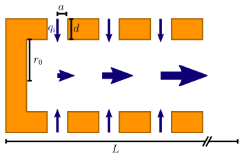
Figure 2: A sketchl of the flow in the membrane pores showing a tube with pores of radius $a$ and length $d$.

The total resistance $R$ of $N$ non-interacting pores in parallel is related to the permeability $L_{p}$ of the membrane as

$$\frac{1}{R}=\frac{N}{R_{i}}=\frac{N\pi a^{4}}{8\eta d}\equiv 2\pi r_{0}LL_{p}$$ (42)

giving the relation

$$L_{p}=\frac{na^{4}}{16\eta dr_{0}}.$$ (43)

or

$$k=\eta L_{p}d=\frac{na^{4}}{16r_{0}}.$$ (44)

The dissipation inside the pore is dependent on the choice of pore radius $a$ and covering fraction $\phi$, since this determines the actual inflow velocity $v_{i}$ through pore number $i$ and the corresponding flux $q_{i}=\pi a^{2}v_{i}$. They are connected to the continuous inflow $v_{0}(x)$ as

$$v_{0}(x)=\phi\,v_{i}.$$ (45)

with the covering fraction

$$\phi=\frac{n\pi a^{2}}{2\pi r_{0}}=\frac{na^{2}}{2r_{0}},$$ (46)

in terms of which

$$L_{p}=\frac{\phi a^{2}}{4\eta d},$$ (47)

and

$$k=\eta L_{p}d=\frac{1}{4}\phi a^{2},$$ (48)

The viscous dissipation through all pores in the membrane is (by (19))

$$\dot{W}_{\text{mem}} =\frac{8\eta d}{\pi a^{4}}\sum_{i=1}^{N}q_{i}^{2}$$

$$=\frac{8\eta d}{\pi a^{4}}\frac{n\pi^{2}a^{4}}{\phi^{2}}\int_{0}^{L}v_{0}^{2}(x)dx$$

$$=\frac{2\pi r_{0}}{L_{p}}\int_{0}^{L}v_{0}^{2}(x)dx$$ (49)

$$=\frac{1}{2\pi r_{0}L_{p}}\int_{0}^{L}\left(Q^{\prime}(x)\right)^{2}dx.$$ (50)

One might wonder, whether it is valid to retain this term compared to the terms in Eq. (21), which we discarded. In particular, the first term in (21) has precisely the same form as (50), but with a different prefactor. However, $L_{p}$ is assumed to be small due to the smallness of $a/r_{0}$ and $\phi$. The ratio of this latter term to (50) is roughly $(\eta/r_{0}^{2})r_{0}L_{p}=\eta L_{p}/r_{0}=\phi a^{2}/(4r_{0})$. The covering fraction $\phi$ must be less than unity (typically it is much less) and since $a/d<1$ and $a/r_{0}\ll 1$ this ratio is typically very small.

References

- LaBarbera (1990) M. LaBarbera, Science 249, 992 (1990).
- Holbrook and Zwieniecki (2005) N. M. Holbrook and M. Zwieniecki, eds., Vascular transport in plants (Academic Press, 2005).
- Batchelor (2000) G. K. Batchelor, An Introduction to Fluid Dynamics (Cambridge University Press, 2000) p. 660.
- Marbach and Bocquet (2016) S. Marbach and L. Bocquet, Physical Review X 6, 031008 (2016).
- Jensen et al. (2016) K. H. Jensen, K. Berg-Sørensen, H. Bruus, N. M. Holbrook, J. Liesche, A. Schulz, M. A. Zwieniecki, and T. Bohr, Reviews of Modern Physics 88, 035007 (1 (2016).
- Nielsen (2012) C. H. Nielsen, ed., Biomimetic Membranes for Sensor and Separation Applications (Springer, 2012).
- Berman (1953) A. S. Berman, Journal of Applied Physics 24, 1232 (1953).
- Schlichting and Gersten (2000) H. Schlichting and K. Gersten, Boundary Layer Theory (Springer, 2000) p. 824.
- Yuan and Finkelstein (1956) S. W. Yuan and A. B. Finkelstein, Trans ASME 78, 719 (1956).
- Aldis (1988) G. Aldis, Bulletin of Mathematical Biology 50, 547 (1988).
- Berman (1958) A. Berman, Journal of Applied Physics 29, 71 (1958).
- Cox (1991) S. Cox, Journal of Fluid Mechanics 227, 1 (1991).
- King and Cox (2001) J. R. King and S. M. Cox, , 87 (2001).
- Majdalani and Zhou (2003) J. Majdalani and C. Zhou, Zamm 83, 181 (2003).
- Dauenhauer and Majdalani (2003) E. C. Dauenhauer and J. Majdalani, Physics of Fluids 15, 1485 (2003).
- Kurdyumov (2008) V. N. Kurdyumov, Physics of Fluids 20, 123602 (2008).
- Saad and Majdalani (2009) T. Saad and J. Majdalani, Proceedings of the Royal Society A: Mathematical, Physical and Engineering Sciences 466, 331 (2009).
- Xu et al. (2010) H. Xu, Z.-L. Lin, S.-J. Liao, J.-Z. Wu, and J. Majdalani, Physics of Fluids 22, 053601 (2010).
- Liu and Prosperetti (2011) Q. Liu and A. Prosperetti, Journal of Fluid Mechanics 679, 77 (2011).
- Fermi (1956) E. Fermi, Thermodynamics (Dover, 1956).
- Landau and Lifshitz (1987) L. D. Landau and E. M. Lifshitz, Fluid Mechanics, 2nd edition (Pergamon Press, 1987).
- Rademaker et al. (2017) H. Rademaker, M. A. Zwieniecki, T. Bohr, and K. H. Jensen, Physical Review E 95, 042402 (2017).
- Landsberg and Fowkes (1978) J. J. Landsberg and N. D. Fowkes, Annals of Botany 42, 493 (1978).