Towards Asymptotically Optimal One-to-One PDP Algorithms for Capacity 2+ Vehicles

Abstract

We consider the one-to-one Pickup and Delivery Problem (PDP) in Euclidean Space with arbitrary dimension $d$ where $n$ transportation requests are picked i.i.d. with a separate origin-destination pair for each object to be moved. First, we consider the problem from the customer perspective where the objective is to compute a plan for transporting the objects such that the Euclidean distance traveled by the vehicles when carrying objects is minimized. We develop a polynomial time asymptotically optimal algorithm for vehicles with capacity $o(\sqrt[2d]{n})$ for this case. This result also holds imposing LIFO constraints for loading and unloading objects. Secondly, we extend our algorithm to the classical single-vehicle PDP where the objective is to minimize the total distance traveled by the vehicle and present results indicating that the extended algorithm is asymptotically optimal for a fixed vehicle capacity if the origins and destinations are picked i.i.d. using the same distribution.

1 Introduction

The challenge of computing optimal or near-optimal plans for transporting goods or people is a core challenge within logistics. This problem has received a huge amount of attention from the operations research community. A generic term for this class of problems is Vehicle Routing Problems. Vehicle routing problems come in many flavors depending among other things on the properties of the vehicles used, the characteristics of the terrain and the type of transportation requests considered.

In this paper, we consider the variant of the problem where the terrain is the Euclidean space of an arbitrary dimension $d$ and where we measure the distance using the Euclidean distance. We have one vehicle with limited capacity at our disposal but the vehicle can carry more than one object at a time. Every object to be transported has a separate origin and destination. The objective is to compute a plan for transporting the objects with a minimum distance traveled by the vehicle. We look at the nonpreemptive version meaning that an object has to stay on the vehicle until it is delivered. Our version is static (offline) in the sense that all information on the transportation requests is available to us before we have to compute the optimal route for the vehicle.

The origins and destinations are picked using a stochastic process and we measure the performance of an algorithm by considering the approximation ratio, i.e. the value of the solution computed by the algorithm divided by the value of the optimal solution. The main aim of the paper is to present polynomial time algorithms that are asymptotically optimal in the sense that the approximation ratio converges to $1$ with probability $1$ (almost surely) as the number of transportation requests goes to infinity. To the best of our knowledge, we are the first to present asymptotically optimal algorithms for the realistic setting where the vehicles have a limited capacity greater than one. Our algorithms are easy to implement and they may be useful in practice.

1.1 Related Work

In the literature, the problem considered is often referred to as the One-to-One Pickup and Delivery Problem (PDP) or the Vehicle Routing Problem with Paired Pickups and Deliveries. The single vehicle case that we look at in this paper is also known as the Traveling Salesman Problem with Pickups and Deliveries because this case can be viewed as a Traveling Salesman Problem (TSP) with precedence constraints where the origin of an object must be visited before the corresponding destination. If the single vehicle has capacity $1$ then this problem is known as the Stacker Crane Problem (SCP). We refer the reader to the excellent surveys  [3, 10, 11, 13] for an overview on vehicle routing research.

The PDP problem in focus in this paper is defined as follows:

Definition 1.

An instance of the PDP problem for dimension $d$ and capacity $c$ is a set of $n$ requests $R=\{r_{1},r_{2},\ldots,r_{n}\}$ with $r_{i}\in[0,1]^{d}\times[0,1]^{d}$ for $i\in\{1,2,\ldots,n\}$. A request $r=(s,t)$ corresponds to a transportation job for an object with origin $s$ and destination $t$. The solution is a plan for transporting all objects from their origin to their destination minimizing the total Euclidean distance traveled using a single vehicle with capacity $c$. The vehicle is initially at $(0,0,\ldots,0)$.

As noted by many authors, the PDP problem generalizes the classical TSP problem and is thus NP complete for $d\geq 2$. Guan [7] has shown that the PDP problem is NP complete for $d=1$ and $c\geq 2$ and Guan also shows how to solve this version in linear time if we allow temporarily dropping objects. Treleaven et al. [15] present asymptotically optimal algorithms for $c=1$ (SCP) and $d\geq 2$ where the origins are picked i.i.d. and the destinations are picked i.i.d. from separate distributions.

Stein [14] also conducts a probabilistic analysis but he looks at the variant where $d=2$ and $c=+\infty$ and where $n$ origins and $n$ destinations are picked independently using a uniform distribution on some planar region. Stein shows that the value of the optimal solution divided by $\sqrt{n}$ converges almost surely to a constant times the square root of the area of the region. Stein also shows how to solve the problem he considers by concatenating two TSP tours on the origins and destinations respectively. This way of solving the problem yields a solution which is roughly $6\%$ higher than the optimal solution (in the limit).

Psaraftis [12] has developed an $O(n^{2})$ heuristic guaranteeing an approximation ratio of at most $4$ for any instance for the case $d=2$ and $c=+\infty$. Haimovich and Kan [8] have constructed asymptotically optimal PDP algorithms for the case $d=2$ where all transportation requests have the same depot as destination. Haimovich and Kan [8] also presented a PTAS for this case for $c=O(\log\log n)$ and this result has later been extended to cover cases with multiple depots and arbitrary values of $d$ [9] or larger values of $c$ [5].

In some cases, the customers only pay for a kilometer driven by the vehicle if the vehicle carries an object when driving that kilometer. As an example, this is the case when the vehicles are taxis. This leads us to the PDP-C problem that does not seem to have received much attention:

Definition 2.

The PDP-C problem is identical to the PDP problem with the exception that distance traveled carrying no objects is excluded.

The PDP-C problem covers any situation where carrying objects is very expensive compared to carrying no objects. Possible areas for application are the development of taxi sharing or ride sharing schemes. The PDP-C problem also comes into play when we want to minimize the time spent for an elevator (or robot arm) that moves slowly carrying passengers (objects) but moves very fast carrying no passengers (objects).

An efficient and near-optimal subroutine solving the PDP-C problem might also be useful in the case where we have multiple vehicles at our disposal and the objective is to minimize the completion time (the time when the last object has been delivered). A first step to solve this problem could involve partitioning objects into groups sharing a vehicle using a PDP-C subroutine.

1.2 Contribution and Outline

In Section 2, we present an adaptive asymptotically optimal polynomial time algorithm for the PDP-C problem for $c=o(\sqrt[2d]{n})$ for any dimension $d$ under the assumption that the transportation requests are picked independently and by identical distributions (i.i.d.). As explained above, there are many real world problems where a PDP-C algorithm is useful.

A PDP algorithm is presented in Section 3 accompanied by what we consider to be good reasons to believe that this algorithm is asymptotically optimal for a constant capacity $c$ if the origins and destinations for the transportation requests are picked i.i.d. using the same distribution. The PDP algorithm is an extension of our PDP-C algorithm.

The key idea for our approach is that we solve a TSP with precedence constraints in $d$-dimensional Euclidean space – the PDP problem – by solving a classical TSP defined by the requests in Euclidean space with the double dimension $2d$. Neighbors in the solution to the classical TSP correspond to objects that have similar requests so we let such neighbors share a vehicle.

As mentioned earlier, we believe that we are the first to present results on asymptotic optimality for the realistic case $1<c<+\infty$. Our results also hold if we allow temporarily dropping objects (the preemptive variant) or if we impose LIFO constraints for loading and unloading objects.

2 An Asymptotically Optimal PDP-C Algorithm

In this section, we present our PDP-C algorithm. We begin by listing the pseudocode consisting of $4$ steps. We also exemplify how the steps work using the instance shown in Fig. 1 that has $d=1$ and $c=2$.

2.1 The Pseudocode

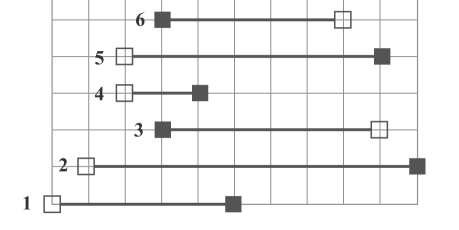
Figure 1: An instance of a $1$-dimensional PDP-C problem. The white and black squares correspond to pickups and deliveries respectively. As an example, request $4$ shows that an object has to be picked up at $0.2$ and delivered at $0.4$. We assume that vehicles with capacity $2$ are used.

Throughout the paper, we assume that $n=mc$ for some integer $m$. Otherwise, we can serve the extra objects one by one implying an extra $O(c)$ cost that does not affect our results on asymptotic optimality.

Step $1$

Use a polynomial time constant factor approximation algorithm [1, 4] to compute a feasible solution $T$ for the $2d$-dimensional Euclidean TSP problem defined by $R$ ($\sigma$ is a permutation on $\{1,2,\ldots,n\}$):

$$T=r_{\sigma(1)}\rightarrow r_{\sigma(2)}\rightarrow\ldots\rightarrow r_{\sigma(n)}\rightarrow r_{\sigma(1)}\enspace.$$

The tour $T$ is shown in Fig. 2.

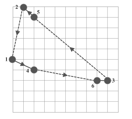
Figure 2: The objects that are to be transported live in $1$-dimensional Euclidean space. The requests from Fig. 1 are members of the $2$-dimensional Euclidean space. As an example, request $4$ is the point $(0.2,0.4)\in[0,1]^{2}$. The PDP-C algorithm attacks a $1$-dimensional PDP-C problem by solving a classical $2$-dimensional TSP defined by the requests. The two ways to split $T$ into groups are indicated by the dashed and solid arrows respectively.

Step $2$

We now split $T$ into $m$ groups such that each group contains $c$ consecutive requests $r_{\sigma(i)},r_{\sigma(i+1)},\ldots,r_{\sigma(i+c-1)}$. One possible way of partitioning the requests into groups is as follows:

$$\{r_{\sigma(1)},r_{\sigma(2)},\ldots,r_{\sigma(c)}\},$$

$$\{r_{\sigma(c+1)},r_{\sigma(c+2)},\ldots,r_{\sigma(2c)}\},$$

$$\ldots$$

$$\{r_{\sigma(n-c+1)},r_{\sigma(n-c+2)},\ldots,r_{\sigma(n)}\}\enspace.$$

There are $c$ ways to do the split up (See Fig. 2). For each of the possibilities, we repeat Step $3$ and obtain $c$ candidate solutions for the PDP-C problem:

Step $3$ (repeated for each possible splitting of $T$)

The objects in a group share a vehicle. The objects for a group of requests $\{r_{\sigma(i)}$, $r_{\sigma(i+1)}$, $\ldots$ , $r_{\sigma(i+c-1)}\}$ are picked up in the order $\sigma(i)$, $\sigma(i+1)$, …, $\sigma(i+c-1)$ and dropped off in reverse order (LIFO). The plan corresponding to one of the ways to split $T$ into groups is shown in Fig. 3.

Step $4$

Finally, we pick the best of the $c$ candidate solutions produced in Step $3$. The plan computed by the algorithm is shown in Fig. 3.

Figure 3: The feasible solution for the PDP-C instance computed by the PDP-C algorithm. The solution is based on the splitting of $T$ indicated by solid arrows in Fig. 2. The objects are picked up and dropped in LIFO order.

2.2 Analysis of the PDP-C Algorithm

We let $SOL$ denote the value of the plan computed by the PDP-C algorithm. We kindly remind the reader that the value is the Euclidean distance traveled where we only measure the distance traveled carrying objects. The value of the optimal solution is denoted by $OPT$. The length of the tour $T$ is $\|T\|_{2d}$ where the subscript indicates the dimension of the underlying Euclidean space.

We now present a key lemma that links the TSP in $2d$-space to the value of the solution computed by the PDP-C algorithm:

Lemma 1.

$$SOL\leq\sum_{i=1}^{n}\frac{\|s_{i}-t_{i}\|_{d}}{c}+\sqrt{2}\left(\frac{c-1}{c}\right)\|T\|_{2d}\enspace.$$ (1)

Proof.

Let $SOL_{i}$, $i\in\{1,2,\ldots,c\}$, denote the Euclidean distance covered for the $i$’th plan computed by Step $3$. The sum $\sum_{i=1}^{c}SOL_{i}$ can be broken down into three terms:

$$\sum_{i=1}^{c}SOL_{i}=P+F+D\enspace$$ (2)

where $P$ is a term for picking up objects, $F$ is a term for driving with a full vehicle, and $D$ is a term for dropping off objects. Every object tries to be the final object to be picked up in precisely one of the plans:

$$F=\sum_{i=1}^{n}\|s_{i}-t_{i}\|_{d}\enspace.$$ (3)

The segments $s_{\sigma(i)}\rightarrow s_{\sigma(i+1)}$ and $t_{\sigma(i+1)}\rightarrow t_{\sigma(i)}$ are traversed in exactly $c-1$ of the plans, $i\in\{1,2,\ldots,n\}$ (Addition is performed cyclically: $n+1=1$):

$$P+D=(c-1)\sum_{i=1}^{n}\left[\|s_{\sigma(i)}-s_{\sigma(i+1)}\|_{d}+\|t_{\sigma(i)}-t_{\sigma(i+1)}\|_{d}\right]\enspace.$$ (4)

The key to connecting the $d$-dimensional space to the $2d$-dimensional space is the following simple observation that follows from the elementary identity $\sqrt{x}+\sqrt{y}\leq\sqrt{2}\sqrt{x+y}$:

$$\|s_{\sigma(i)}-s_{\sigma(i+1)}\|_{d}+\|t_{\sigma(i)}-t_{\sigma(i+1)}\|_{d}\leq\sqrt{2}\|r_{\sigma(i)}-r_{\sigma(i+1)}\|_{2d}\enspace.$$ (5)

We now combine the two preceding facts:

$$P+D\leq\sqrt{2}(c-1)\|T\|_{2d}\enspace.$$ (6)

The Lemma now follows from

$$SOL\leq\frac{1}{c}\sum_{i=1}^{c}SOL_{i}\enspace.$$ (7)

∎

We are now ready to prove that our PDP-C algorithm is asymptotically optimal:

Theorem 1.

Let an infinite sequence of requests $(s_{i},t_{i})$ be picked i.i.d. in $[0,1]^{d}\times[0,1]^{d}$ using a distribution satisfying that $E[\|s_{i}-t_{i}\|_{d}]=\mu>0$. Let $SOL_{n}$ denote the value of the plan computed by the PDP-C algorithm and let $OPT_{n}$ denote the value of the optimal plan for the first $n$ requests. If $c=o(\sqrt[2d]{n})$ then we have the following:

$$\lim_{n\rightarrow+\infty}\frac{SOL_{n}}{OPT_{n}}=1\mbox{ a.s.}$$ (8)

Proof.

The objects could share the bill of traveling by equally sharing the cost for each segment. This sharing scheme leads to the following lower bound on $OPT_{n}$:

$$OPT_{n}\geq\sum_{i=1}^{n}\frac{\|s_{i}-t_{i}\|_{d}}{c}$$ (9)

We now combine the lower bound on $OPT_{n}$ with Lemma 1:

$$\frac{SOL_{n}}{OPT_{n}}\leq 1+\sqrt{2}(c-1)\left(\sum_{i=1}^{n}\|s_{i}-t_{i}\|_{d}\right)^{-1}\|T\|_{2d}\enspace.$$ (10)

The inequality (10) is rewritten slightly:

$$\frac{SOL_{n}}{OPT_{n}}\leq 1+\sqrt{2}(c-1)\left(\frac{\sum_{i=1}^{n}\|s_{i}-t_{i}\|_{d}}{n}\right)^{-1}\frac{\|T\|_{2d}}{n}\enspace.$$ (11)

We use a constant factor approximation algorithm for solving the TSP in $2d$-dimensional space implying this upper bound on the length of $T$ [6]:

$$\|T\|_{2d}=O(n^{\frac{2d-1}{2d}})\enspace.$$ (12)

Using $c=o(\sqrt[2d]{n})$, we now get the following:

$$c\|T\|_{2d}=o(n)\enspace.$$ (13)

According to the Strong Law of Large Numbers, we have the following:

$$\lim_{n\rightarrow+\infty}\left(\frac{\sum_{i=1}^{n}\|s_{i}-t_{i}\|_{d}}{n}\right)^{-1}=\mu^{-1}\mbox{ a.s.}$$ (14)

The lemma now follows from (11), (13) and (14). ∎

A few comments on the convergence rate might be suitable at this point. According to [2], the limit of $\frac{\|T\|_{2d}}{n}\sqrt[2d]{n}$ is almost surely a constant where the constant depends on the distribution of the requests with maximum value for the uniform distribution. In other words, the algorithm is adaptive in the sense that the right hand side of (11) tends to be smaller for big instances for the non-uniform case.

Even for relatively small values of $n$, we might experience a right hand side of (11) that is relatively close to $1$. As an example, we consider the case $d=1$ where we admittedly have the best conditions for convergence. Few [6] has shown that $\|T\|_{2}\leq\sqrt{2n}+\frac{7}{4}$ implying that the right hand side of (11) converges relatively quickly to $1$ for moderate $c$ for the case $d=1$ if $\mu$ is not too small.

3 A PDP Algorithm

We now turn our attention to the PDP problem and present a polynomial time algorithm that can be viewed as a generalization of the Iterated Tour Partition Heuristic that Haimovich and Kan [8] presented for the case where $d=2$ and all the destinations are identical. The tour that we consider is a tour in $2d$-dimensional Euclidean space where the requests are members and we allow different destinations for arbitrary $d$.

Our PDP algorithm is an extension of our PDP-C algorithm: First, we figure out what objects should share the vehicle and establish a LIFO order for pickups and deliveries (PDP-C with $1<c<+\infty$). Secondly, we set up a route for the vehicle focusing on the segments when it carries no objects (PDP with $c=1$. SCP in other words). We exemplify our PDP algorithm by adding two more figures to the PDP-C example. The pseudocode for the PDP algorithm consists of the following $6$ steps:

Steps $1-4$

Use the steps from the PDP-C Algorithm and compute a PDP-C solution.

Step $5$

Use an algorithm from the SPLICE class [15] to compute a feasible solution $S$ for the SCP instance defined by a pickup at the origin and a delivery at the destination for every object that was the first to be picked up by a vehicle (and consequently the last object to be dropped off) in the PDP-C solution. Let $S_{0}$ denote the set of segments that go from a delivery to a pickup from the solution $S$ to the Stacker Crane Problem. See Fig. 4.

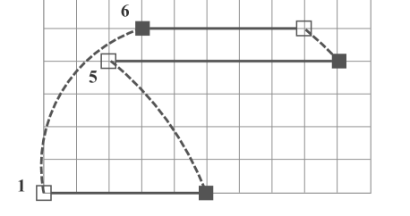
Figure 4: The SCP and the solution $S$ computed in Step $5$. The dashed segments are the segments in $S_{0}$. The objects for the requests $1$, $5$ and $6$ where the first to be picked up in the PDP-C solution in Fig. 3.

Step $6$

A PDP solution can now be produced by combining the PDP-C solution with the segments $S_{0}$ from the Stacker Crane Plan where no objects where carried. See Fig. 5.

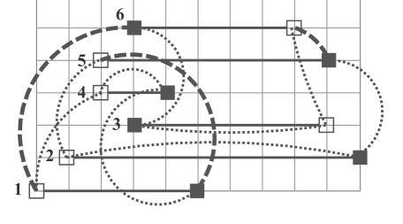
Figure 5: The solution for the PDP problem computed by the PDP algorithm.

We now let $SOL$ denote the total Euclidean distance covered by the vehicle for the plan proposed by the PDP algorithm. The optimal solution is denoted by $OPT$. The total length of the delivery-to-pickup segments from $S$ that we use in Step $6$ is $\|S_{0}\|_{d}$ where $d$ refers to the dimension of the Euclidean space.

Lemma 2.

$$SOL\leq\sum_{i=1}^{n}\frac{\|s_{i}-t_{i}\|_{d}}{c}+\sqrt{2}\left(\frac{c-1}{c}\right)\|T\|_{2d}+\|S_{0}\|_{d}\enspace.$$ (15)

Proof.

Compared to Lemma 1 the extra distance driven is $\|S_{0}\|_{d}$. ∎

Observation 1.

If the following conditions are met

$$c\|S_{0}\|_{d}=o(n)\enspace,$$ (16)

$$c\|T\|_{2d}=o(n)\enspace,\mbox{ and }$$ (17)

$$\sum_{i=1}^{n}\|s_{i}-t_{i}\|_{d}=\Omega(n)\enspace,$$ (18)

then the PDP Algorithm is asymptotically optimal: $\lim_{n\rightarrow+\infty}\frac{SOL_{n}}{OPT_{n}}=1$.

It follows from [15] that $\|S_{0}\|_{d}$ is $o(n)$ almost surely for $d\geq 3$ if $S$ is the Stacker Crane tour computed by a SPLICE algorithm on $n$ requests in $[0,1]^{d}\times[0,1]^{d}$ with the origins and destinations picked i.i.d. using the same distribution. The Stacker Crane tour $S$ from our PDP algorithm consists of $n/c$ requests but the corresponding points are not picked independently. Informally speaking, these $n/c$ requests seem to be spread evenly on $R$ so we are optimistic with respect to proving that (16) holds but more work has to be done to look into the details and conditions for convergence. Observation 1 gives us reason to believe that our PDP algorithm is asymptotically optimal for fixed capacity $c$ if the origins and destinations are picked i.i.d. from the same distribution since (17) and (18) hold in this case and (16) seems plausible.

Conclusion

We have presented a polynomial time asymptotically optimal algorithm for the PDP-C problem and a polynomial time algorithm for the PDP problem that we have good reasons to believe is asymptotically optimal as well (under certain assumptions for picking the transportation requests). Our results are dealing with vehicles with limited capacity greater than one. One obvious idea for future work is incorporating time windows by extending the dimension of the request space.

References

- [1] S. Arora. Polynomial time approximation schemes for euclidean traveling salesman and other geometric problems. J. ACM, 45(5):753–782, September 1998.
- [2] J. Beardwood, J. H. Halton, and J. M. Hammersley. The shortest path through many points. Mathematical Proceedings of the Cambridge Philosophical Society, 55(4):299–327, 1959.
- [3] G. Berbeglia, J. F. Cordeau, I. Gribkovskaia, and G. Laporte. Static pickup and delivery problems: a classification scheme and survey. TOP: An Official Journal of the Spanish Society of Statistics and Operations Research, 15(1):1–31, 2007.
- [4] N. Christofides. Worst-case analysis of a new heuristic for the travelling salesman problem. Technical Report 388, Graduate School of Industrial Administration, Carnegie Mellon University, 1976.
- [5] A. Das and C Mathieu. A quasipolynomial time approximation scheme for euclidean capacitated vehicle routing. Algorithmica, 73(1):115–142, 2015.
- [6] L. Few. The shortest path and the shortest road through n points. Mathematika, 2(2):141–144, 12 1955.
- [7] D.J. Guan. Routing a vehicle of capacity greater than one. Discrete Applied Mathematics, 81(1):41 – 57, 1998.
- [8] M. Haimovich and A. H. G. Rinnooy Kan. Bounds and heuristics for capacitated routing problems. Mathematics of Operations Research, 10(4):527–542, 1985.
- [9] M. Khachay and R. Dubinin. PTAS for the euclidean capacitated vehicle routing problem in . In DOOR 2016, volume 9869 of Lecture Notes in Computer Science, pages 193–205. Springer, 2016.
- [10] S. N. Parragh, K. F. Doerner, and R. F. Hartl. A survey on pickup and delivery problems (part I). Journal für Betriebswirtschaft, 58(1):21–51, 2008.
- [11] S. N. Parragh, K. F. Doerner, and R. F. Hartl. A survey on pickup and delivery problems (part II). Journal für Betriebswirtschaft, 58(2):81–117, 2008.
- [12] H. N. Psaraftis. Analysis of an o(n²) heuristic for the single vehicle many-to-many euclidean dial-a-ride problem. Transportation Research. Part B: Methodological, pages 133–145, 1981.
- [13] M. W. P. Savelsbergh and M. Sol. The general pickup and delivery problem. Transportation Science, 29:17–29, 1995.
- [14] D. M. Stein. An asymptotic, probabilistic analysis of a routing problem. Mathematics of Operations Research, 3(2):89–101, 1978.
- [15] K. Treleaven, M. Pavone, and E. Frazzoli. Asymptotically optimal algorithms for one-to-one pickup and delivery problems with applications to transportation systems. IEEE Transactions on Automatic Control, 58(9):2261–2276, 2013.