Adaptive regularization for Lasso models in the context of non-stationary data streams

Abstract

Large scale, streaming datasets are ubiquitous in modern machine learning. Streaming algorithms must be scalable, amenable to incremental training and robust to the presence of non-stationarity. In this work consider the problem of learning $\ell_{1}$ regularized linear models in the context of streaming data. In particular, the focus of this work revolves around how to select the regularization parameter when data arrives sequentially and the underlying distribution is non-stationary (implying the choice of optimal regularization parameter is itself time-varying). We propose a framework through which to infer an adaptive regularization parameter. Our approach employs an $\ell_{1}$ penalty constraint where the corresponding sparsity parameter is iteratively updated via stochastic gradient descent. This serves to reformulate the choice of regularization parameter in a principled framework for online learning. The proposed method is derived for linear regression and subsequently extended to generalized linear models. We validate our approach using simulated and real datasets and present an application to a neuroimaging dataset.

1 Introduction

We are interested in learning $\ell_{1}$ regularized regression models in the context of streaming, non-stationary data. There has been significant research relating to the estimation of such models in a streaming data context (Bottou, 2010; Duchi et al., 2011). However a fundamental aspect that has been overlooked is the selection of the regularization parameter. The choice of this parameter dictates the severity of the regularization penalty. While the underlying optimization problem remains convex, distinct choices of such a parameter yield models with vastly different characteristics. This poses significant concerns from the perspective of model performance and interpretation. It therefore follows that selecting such a parameter is an important problem that must be addressed in a data-driven manner.

Many solutions have been proposed through which to select the regularization parameter in a non-streaming context. For example, stability based approaches have been proposed in the context of linear regression (Meinshausen and Bühlmann, 2010). Other popular alternatives include cross-validation and information theoretic techniques (Hastie et al., 2015). However, in a streaming setting such approaches are infeasible due to the limited computational resources available. Moreover, the statistical properties of the data may vary over time; a common manifestation being concept drift (Aggarwal, 2007). This complicates the use of sub-sampling methods as the data can no longer be assumed to follow a stationary distribution. Furthermore, as we argue in this work, it is conceivable that the optimal choice of regularization parameter may itself vary over time. It is also important to note that traditional approaches such as change-point detection cannot be employed as there is no readily available pivotal quantity. It therefore follows that novel methodologies are required in order to tune regularization parameters in an online setting.

Applications involving streaming datasets are abundant, ranging from finance to cyber-security (Heard et al., 2010; Gibberd and Nelson, 2014) and neuroscience (Weiskopf, 2012). In this work we are motivated by the latter application, where penalized regression models are often employed to decode statistical dependencies across spatially remote brain regions, referred to as functional connectivity (Smith et al., 2011). A novel avenue for neuroscientific research involves the study of functional connectivity in real-time (Weiskopf, 2012). Such research faces challenges due to the non-stationary as well as potentially high dimensional nature of neuroimaging data (Monti et al., 2014). In order to address these challenges, many of the proposed methods to date have employed fixed sparsity parameters. However, such choices are typically justified only by the methodological constraints associated with updating the regularization parameter, as opposed to for biological reasons.

In order to address these issues we propose a framework through which to learn an adaptive sparsity parameter in an online fashion. The proposed framework, named Real-time Adaptive Penalization (RAP), is capable of iteratively learning time-varying regularization parameters via the use of adaptive filtering. Briefly, adaptive filtering methods are semi-parametric methods which employ information from recent observations to tune a parameter of interest. In this manner, adaptive filtering methods are capable of handling temporal variation which cannot easily be modeled explicitly (Haykin, 2008). The contributions of this work can be summarized as follows:

1. We propose and validate a framework through which to tune a time-varying sparsity parameter for $\ell_{1}$ regularized linear models in real-time.

2. We provide theoretical insights regarding the properties and behavior of the proposed method. 

3. The proposed framework is subsequently extended to the context regularized generalized linear models.

4. An empirical validation is provided using both synthetic and real datasets together with an application to a neuroimaging dataset.

The remainder of this manuscript is organized as follows: related work is discussed in Section 2. We formally describe our problem in Section 3 and the proposed framework is introduced in Section 4. We provide empirical evidence based on real and simulated data in Section 5.

2 Related work

Regularized methods have established themselves as popular and effective tools through which to handle high-dimensional data (Hastie et al., 2015). Such methods employ regularization penalties as a mechanism through which to constraint the set of candidate solutions, often with the goal of enforcing specific properties such as parsimony. In particular, $\ell_{1}$ regularization is widely employed as a convex approximation to the combinatorial problem of model selection.

However, the introduction of an $\ell_{1}$ penalty requires the specification of the associated regularization parameter. The task of tuning such a parameter has primarily been studied in the context of non-streaming, stationary data. Stability selection procedures, introduced by Meinshausen and Bühlmann (2010), effectively look to by-pass the selection of a specific regularization parameter by instead fitting multiple models across sub-sampled data. Variables are subsequently selected according to the proportion of all models in which they are present. In this manner, stability selection is able to provide important theoretical guarantees, albeit while incurring an additional computational burden. Other popular approaches involve the use of cross-validation or information theoretic techniques. However, such methods cannot be easily adapted to handle streaming data.

Online learning with the $\ell_{1}$ constraints has also been studied extensively and many computationally efficient algorithms are available. A stochastic gradient descent algorithm is proposed by Bottou (2010). More generally, online learning of regularized objective functions has been studied extensively by Duchi et al. (2011) who propose a general class of computationally efficient methods based on proximal gradient descent. The aforementioned methods all constitute important advances in the study of sparse online learning algorithms. However, a fundamental issue that has been overlooked corresponds to the selection of the regularization parameters. As such, current methodologies are rooted on the assumption that the regularization parameter remains fixed. It follows that the regularization parameter may itself vary over time, yet selecting such a parameter in a principled manner is non-trivial. The focus of this work is to present and validate a framework through which to automatically select and update the regularization parameter in real-time. The framework presented in this work is therefore complementary and can be employed in conjunction with many of the preceding techniques. In a similar spirit to the methods proposed in this manuscript, Garrigues and Ghaoui (2009) propose a method for selecting the regularization parameter in the context of sequential data but do not consider non-stationary data, which is the explicit focus of this work. We further consider the extension to general linear models, leading to a wider range of potential applications.

More generally, the automatic selection of hyper-parameters has recently become an active topic in machine learning (Shahriari et al., 2016). Interest in this topic has been catalyzed by the success of deep learning algorithms, which typically involve many such hyper-parameters. Sequential model based optimization (SMBO) methods such as Bayesian optimization employ a probabilistic surrogate to model the generalization performance of learning algorithms as samples from a Gaussian process (Shahriari et al., 2016), leading to expert level performance in many cases. It follows that such methods may be employed to tune regularization parameters in the context of penalized linear regression models. However, there are several important differences between the SMBO framework and the proposed framework. The most significant difference relates to the fact that the proposed framework employs gradient information in order to tune the regularization parameter while SMBO methods such as Bayesian optimization are rooted in the use of a probabilistic surrogate model. This allows the SMBO framework to be applied in a wide range of settings while the proposed framework focuses exclusively on Lasso regression models. However, as we describe in this work, the use of gradient information makes the RAP framework ideally suited in the context of non-stationary, streaming data. This is in contrast to SMBO techniques, which typically assume the data is stationary.

3 Preliminaries

In this section we introduce the necessary ingredients to derive the proposed framework. We begin formally defining the problem addressed in this work in Section 3.1. Adaptive filtering methods are introduced in Section 3.2.

3.1 Problem set-up

In this work we are interested in streaming data problems. Here it is assumed that pairs $(X_{t},y_{t})$ arrive sequentially over time, where $X_{t}\in\mathbb{R}^{p\times 1}$ corresponds to a $p$-dimensional vector of predictor variables and $y_{t}$ is a univariate response. The objective of this work is to learn time-varying linear regression models from which to accurately predict future responses, $y_{t+1}$, from predictors, $X_{t+1}$. An $\ell_{1}$ penalty, parameterized by $\lambda\in\mathbb{R}_{+}$, is introduced in order to encourage sparse solutions as well as to ensure the problem is well-posed from an optimization perspective. This corresponds to the Lasso model introduced by Tibshirani (1996). For a given choice of regularization parameter, $\lambda$, time-varying regression coefficients can be estimated by minimizing the following convex objective function:

$$L_{t}(\beta,\lambda)=\sum_{i=1}^{t}w_{i}\left(y_{i}-X_{i}^{T}\beta\right)^{2}+\lambda||\beta||_{1},$$ (1)

where $w_{i}>0$ are weights indicating the importance given to past observations (Aggarwal, 2007). Typically, $w_{i}$ decay monotonically in a manner which is proportional to the chronological proximity of the $i$th observation. For example, weights $w_{i}$ may be tuned using a fixed forgetting factor or a sliding window.

In a non-stationary context, the optimal estimates of regression parameters, $\hat{\beta}_{t}$, may vary over time. The same argument can be posed in terms of the selected regularization parameter, $\lambda$. For example, this may arise due to changes in the underlying sparsity or changes in the signal-to-noise ratio. While there exists a wide range of methodologies through which to update regression coefficients in a streaming fashion, the choice of regularization parameter has been largely ignored. As such, the primary objective of this work is to propose a framework through which to learn time-varying regularization parameter in real-time. The proposed framework seeks to iteratively update the regularization parameter via stochastic gradient descent and is therefore conceptually related to adaptive filtering theory (Haykin, 2008), which we introduce below.

3.2 Adaptive filtering

Filtering, as defined in Haykin (2008), is the process through which information regarding a quantity of interest is assimilated using data measured up to and including time $t$. In many real-time applications, the quantity of interest is assumed to vary over time. The task of a filter therefore corresponds to effectively controlling the rate at which past information is discarded. Adaptive filtering methods provide an elegant method through which to handle a wide range of non-stationary behavior without having to explicitly model the dynamic properties of the data stream.

The simplest filtering methods discard information at a constant rate, for example determined by a fixed forgetting factor. More sophisticated methods are able to exploit gradient information to determine the aforementioned rate. Such methods are said to be adaptive as the rate at which information is discarded varies over time. It follows that the benefits of adaptive methods are particularly notable in scenarios where the quantity of interest is highly non-stationary.

To further motivate discussion, we briefly review filtering in the context of fixed forgetting factors for streaming linear regression. In such a scenario, it suffices to store summary statistics for the mean and sample covariance. For a given fixed forgetting factor $r\in(0,1]$, the sample mean can be recursively estimated as follows:

$$\small\bar{X}_{t}=\left(1-\frac{1}{\omega_{t}}\right)\bar{X}_{t-1}+\frac{1}{\omega_{t}}X_{t},$$ (2)

where $\omega_{t}$ is a normalizing constant defined as:

$$\omega_{t}=\sum_{i=1}^{t}r^{t-i}=r\cdot\omega_{t-1}+1.$$ (3)

Similarly, the sample covariance can be learned iteratively:

$$S_{t}=\left(1-\frac{1}{\omega_{t}}\right)S_{t-1}+\frac{1}{\omega_{t}}(X_{t}-\bar{X}_{t})^{T}(X_{t}-\bar{X}_{t}).$$ (4)

It is clear that the value of $r$ directly determines the adaptivity of a filter as well as its susceptibility to noise. However, in many practical scenarios the choice of $r$ presents a challenge as it assumes some knowledge about the degree of non-stationarity of the system being modeled as well as an implicit assumption that this is constant (Haykin, 2008). Adaptive filtering methods address these issues by allowing $r$ to be tuned online in a data-driven manner. This is achieved by quantifying the performance of current parameter estimates for new observations, $X_{t+1}$. Throughout this work we denote such a measure by $C(X_{t+1})$.

A popular approach is to define $C(X_{t+1})$ to be the residual error on unseen data (Haykin, 2008). Then assuming $\frac{\partial C(X_{t+1})}{\partial r}$ can be efficiently calculated, our parameter of interest can be updated in a stochastic gradient descent framework:

$$r_{t+1}=r_{t}-\epsilon\left.\frac{\partial C(X_{t+1})}{\partial r}\right|_{r=r_{t}}$$ (5)

where $\epsilon$ is a small step-size parameter which determines the learning rate. The objective of this work therefore corresponds to extending adaptive filtering methods to the domain of learning a time-varying regularization parameter for Lasso regression models.

4 Methods

As noted previously, the choice of parameter $\lambda$ dictates the severity of the regularization penalty. Different choices of $\lambda$ result in vastly different estimated models. While several data-driven approaches are available for selecting $\lambda$ in an offline setting, such methods are typically not feasible for streaming data for two reasons. First, limited computational resources pose a practical restriction. Second, data streams are often non-stationary and rarely satisfy iid assumptions required for methods based on the bootstrap (Aggarwal, 2007). Moreover, it is important to note that traditional methods such as change point detection cannot be employed due to the absence of a readily available pivotal quantity for $\lambda$.

We begin by outlining the RAP framework in the linear regression setting in Section 4.1. Section 4.2 outlines the resulting algorithm and computational considerations. We derive some properties of the proposed framework in Section 4.3. Finally, in Section 4.4 we extend the RAP framework to the setting of GLMs.

4.1 Proposed framework

We propose to learn a time-varying sparsity parameter in an adaptive filtering framework. This allows the proposed method to relegate the choice of sparsity parameter to the data. Moreover, by allowing $\lambda_{t}$ to vary over time the proposed method is able to naturally accommodate datasets where the underlying sparsity may be non-stationary.

We define the empirical objective to be the look-ahead negative log-likelihood, defined as:

$$C_{t+1}=C(X_{t+1},y_{t+1})=||y_{t+1}-X_{t+1}\hat{\beta}_{t}(\lambda_{t})||_{2}^{2},$$ (6)

where we write $\hat{\beta}_{t}(\lambda_{t})$ to emphasize the dependence of the estimated regression coefficients on the current value of the regularization parameter, $\lambda_{t}$. Following Section 3.2, the regularization parameter can be iteratively updated as follows:

$$\lambda_{t+1}=G(\lambda_{t})=\lambda_{t}-\epsilon\frac{\partial C_{t+1}}{\partial\lambda_{t}}.$$ (7)

We note that for convenience we write $\frac{\partial C_{t+1}}{\partial\lambda_{t}}$ to denote the derivate of $C_{t+1}$ with respect to $\lambda$ evaluated at $\lambda=\lambda_{t}$ (i.e, $\frac{\partial C_{t+1}}{\partial\lambda}|_{\lambda=\lambda_{t}}$). We note that $\lambda_{t}$ is bounded below by zero, in which case no regularization is applied, and above by $\lambda^{max}_{t}=\max_{j}\left\{|\sum_{i=1}^{t}w_{i}y_{i}X_{i,j}|\right\},$ in which case all regression coefficients are zero (Friedman et al., 2010).

The proposed framework requires only the specification of an initial sparsity parameter, $\lambda_{0}$, together with a stepsize parameter, $\epsilon$. In this manner the proposed framework effectively replaces a fixed sparsity parameter with a stepsize parameter, $\epsilon$. This is desirable as the choice of a fixed sparsity parameter is difficult to justify in the context of streaming, non-stationary data. Moreover, any choice of $\lambda$ is bound to be problem specific. In comparison, we are able to interpret $\epsilon$ as a stepsize parameter in a stochastic gradient descent scheme. As a result, there are clear guidelines which can be followed when selecting $\epsilon$ (Bottou, 1998).

Once the regularization parameter has been updated, estimates for the corresponding regression coefficients can be obtained by minimizing $L_{t+1}(\beta,\lambda_{t+1})$, for which there is a wide literature available (Bottou, 2010; Duchi et al., 2011). The challenge in this work therefore corresponds to efficiently calculating the derivative in equation (7). Through the chain rule, this can be decomposed as:

$$\frac{\partial C_{t+1}}{\partial\lambda_{t}}=\frac{\partial C_{t+1}}{\partial\hat{\beta}_{t}}\cdot\frac{\partial\hat{\beta}_{t}}{\partial\lambda_{t}}.$$ (8)

The first term in equation (8) can be obtained by direct differentiation. In the case of the second term, we leverage the results of Efron et al. (2004) and Rosset and Zhu (2007) who demonstrate that the Lasso solution path is piecewise linear as a function of $\lambda$. By implication, $\frac{\partial\hat{\beta}_{t}}{\partial\lambda_{t}}$ must be piecewise constant. Furthermore, there is a simple, closed-form solution for $\frac{\partial\hat{\beta}_{t}}{\partial\lambda_{t}}$.

Proposition 1.

[Adapted from Rosset and Zhu (2007)] In the context of $\ell_{1}$ penalized linear regression models, the derivative $\frac{\partial\hat{\beta}_{t}}{\partial\lambda_{t}}$ is piecewise constant and can be obtained in closed form.

Proof.

For any choice of regularization parameter, $\lambda$, we write $\hat{\beta}_{t}(\lambda)$ to denote the minimizer of equation (1). Recall that the objective, $L_{t}(\beta,\lambda)$, is non-smooth due to the presence of the $\ell_{1}$ penalty. As a result, the sub-gradient of $L_{t}(\beta,\lambda)$ must satisfy:

$$\nabla_{\beta}\left(L_{t}(\beta,\lambda)\right)|_{\beta=\hat{\beta}_{t}(\lambda)}=-X_{1:t}^{T}Wy_{1:t}+X_{1:t}^{T}WX_{1:t}\hat{\beta}_{t}(\lambda)+\lambda~{}\mbox{sign}(\hat{\beta}_{t}(\lambda))\ni 0,$$ (9)

where we $W$ is a diagonal matrix with elements $w_{i}$ and we write $X_{1:t}$ to denote a matrix where the $i$th row is $X_{i}$. It is important to note that equation (9) holds for any choice of $\lambda$, however, the corresponding estimate of regression coefficients, $\hat{\beta}_{t}(\lambda)$, will necessarily change. Further, taking the derivative with respect to the regularization parameter $\lambda$ yields:

$$\frac{\partial}{\partial\lambda}\left(\nabla_{\beta}L_{t}(\beta,\lambda)|_{\beta=\hat{\beta}_{t}(\lambda)}\right) =0$$

$$=\frac{\partial\hat{\beta}_{t}(\lambda)}{\partial\lambda}\nabla_{{}_{\beta}}^{2}L_{t}(\hat{\beta}_{t}(\lambda),\lambda)+\mbox{sign}(\hat{\beta}_{t}(\lambda))$$

$$=\frac{\partial\hat{\beta}_{t}(\lambda)}{\partial\lambda}\left(X_{1:t}^{T}WX_{1:t}\right)+\mbox{sign}(\hat{\beta}_{t}(\lambda)).$$

Rearranging yields:

$$\frac{\partial\hat{\beta}_{t}(\lambda)}{\partial\lambda}=-\left(X^{T}_{1:t}WX_{1:t}\right)^{-1}~{}\mbox{sign}(\hat{\beta}_{t}(\lambda))=-(S_{t})^{-1}~{}\mbox{sign}(\hat{\beta}_{t}(\lambda)).$$ (10)

∎

From Proposition 1 we have that the derivative, $\frac{\partial C_{t+1}}{\partial\lambda_{t}}$, can be computed in closed form. Moreover, we note that the derivative in equation (10) is only non-zero over the active set of regression coefficients, $\mathcal{A}_{t}=\{i:(\hat{\beta}_{t}(\lambda_{t}))_{i}\neq 0\}$, and zero elsewhere. In practice we must therefore consider two scenarios:

• the active set is non-empty (i.e., $\mathcal{A}_{t}\neq\emptyset$). In this case equation (10) is well-defined.

• the active set is empty. In this case we proceed to take a step in the direction of the most correlated predictor: $\hat{j}=\underset{j}{\operatorname{argmax}}\left\{|\sum_{i=1}^{t}w_{i}y_{i}X_{i,j}|\right\}.$ This is equivalent to the first step of the LARS algorithm (Efron et al., 2004).

4.2 Streaming Lasso regression

At each iteration, a new pair $(X_{t+1},y_{t+1})$ is received and employed to update both the time-varying regularization parameter, $\lambda_{t}$, as well as the corresponding estimate of regression coefficients, $\hat{\beta}_{t}(\lambda_{t})$. The former involves computing the derivative $\frac{\partial C_{t+1}}{\partial\lambda_{1}}$ as outlined in Section 4.1. The latter involves solving a convex optimization problem which can be addressed in a variety of ways. In this work we look to iteratively estimate regression coefficients using coordinate descent methods (Friedman et al., 2010). Such methods are easily amenable to streaming data and allow us to exploit previous estimates as warm starts. In our experience, the use of warm starts leads to convergence within a handful of iterations. Pseudo-code detailing the proposed RAP framework is given in Algorithm 1.

Algorithm 1 Real-time Adaptive Penalization

1:$\epsilon\in\mathbbm{R}_{+}$ and $r\in(0,1]$

2:for $t\leftarrow 1\ldots t,\ldots$ do

3:     receive new $(X_{t+1},y_{t+1})$

4:     compute $\frac{\partial\hat{\beta}_{t}(\lambda)}{\partial\lambda_{t}}$ using equation (10)

5:     set $\frac{\partial C_{t+1}}{\partial\lambda_{t}}=\frac{\partial C_{t+1}}{\partial\hat{\beta}_{t}(\lambda)}\frac{\partial\hat{\beta}_{t}(\lambda)}{\partial\lambda_{t}}$

6:     update $\lambda_{t+1}=\lambda_{t}-\epsilon\frac{\partial C_{t+1}}{\partial\lambda_{t}}$

7:     $\hat{\beta}_{t+1}(\lambda_{t+1})=\underset{\beta}{\operatorname{argmin}}\left\{L_{t+1}(\beta,\lambda_{t+1})\right\}$

4.2.1 Computational considerations

With respect to the computational and memory demands, the major expense incurred when calculating $\frac{\partial\hat{\beta}_{t}(\lambda)}{\partial\lambda_{t}}$ involves inverting the sample covariance matrix. The need to compute and store the inverse of the sample covariance is undesirable in the context of high-dimensional data. As a result, the following approximation is also considered:

$${\frac{\partial\hat{\beta}_{t}(\lambda)}{\partial\lambda_{t}}}\approx-\left(\mbox{diag}\left(S_{t}\right)\right)^{-1}~{}\mbox{sign}\left(\hat{\beta}_{t}(\lambda)\right).$$ (11)

Such approximations are frequently employed in streaming or large data applications (Duchi et al., 2011). The approximate update therefore has a time and memory complexity that is proportional to the cardinality of the active set, $\mathcal{A}_{t}$.

4.3 Properties of the proposed framework

In this section we study the properties of the proposed framework. We begin by showing that it is possible to divide the support of the regularization parameter into a finite number of open subsets such that the update rule is piecewise contractive within each subset. We further show that any periodic behavior across adjacent subsets must also be contractive. Unfortunately, as the support of $\lambda$ is divided into open subsets, this precludes the use of Banach’s fixed point theorem. Nonetheless, the properties detailed in this section provide important insights into the proposed framework.

We define $G(\lambda_{t})=\lambda_{t}-\epsilon\frac{\partial C_{t+1}}{\partial\lambda_{t}}$ to be the self-mapping defined on the support $\Lambda=[0,\lambda^{max}_{t}]$. We study the behavior of iteratively applying the update rule $G(\lambda_{t})$ for fixed new data pair $(X_{t+1},y_{t+1})$. This corresponds to iteratively performing the gradient descent update to minimize negative log-likelihood, $C_{t+1}$, for some fixed unseen pair, ($X_{t+1},y_{t+1}$). While the proposed algorithm is stochastic in the sense that distinct random samples, ($X_{t+1},y_{t+1}$), are employed at each update step, the results presented below provide reassuring insights. We note that such non-stochastic results are often presented when studying online algorithms. Throughout the remainder of this section we abuse notation and write $\lambda_{t+1}=G(\lambda_{t})$ to denote the result of applying the gradient update for $t$ iterations. Finally, for any value of $\lambda\in\Lambda$, we write $\mathcal{A}(\lambda)$ to denote the set of active regression coefficients.

First, we demonstrate that the support of the regularization parameter, $\Lambda$, can be divided into a finite number of open subsets where $G$ is a contraction mapping. We then study periodic mappings across pairs of subsets to show that such behavior is itself non-expansive.

Remark 1.

The support of the regularization parameter, $\Lambda$, can be divided into finitely many subsets, $\{S_{i}\}$, such that the active set within each subset is constant.

Remark 1 is a widely used property of the Lasso and is related to the maximum number of iterations performed by the LARS algorithm (Tibshirani, 2013).

Lemma 1.

The support of the regularization parameter can be divided into a finite number of open subsets, $\left\{S_{i}\right\}$, where $G$ is a contraction mapping.

Proof.

From Remark 1 we note that the support of the regularization parameter can be divided into a finite number of open subsets. It remains to show that $G$ is a contraction within each subset.

We consider $\lambda_{1},\lambda_{2}\in S_{i}$ for some $i$. We assume without loss of generality that $\lambda_{1}>\lambda_{2}$. We consider:

$$|G(\lambda_{1})-G(\lambda_{2})|=\left|\lambda_{1}-\lambda_{2}-\epsilon\left(\frac{\partial C_{t+1}}{\partial\lambda_{1}}-\frac{\partial C_{t+1}}{\partial\lambda_{2}}\right)\right|.$$ (12)

Our objective is to show that $\frac{\partial C_{t+1}}{\partial\lambda_{1}}-\frac{\partial C_{t+1}}{\partial\lambda_{2}}>0$, thereby showing that $G$ is a contraction for suitably chosen $\epsilon$. The gradient with respect to regularization parameter $\lambda$ is defined as:

$$\frac{\partial C_{t+1}}{\partial\lambda}=\left(y_{t+1}-X_{t+1}\hat{\beta}_{t}(\lambda)\right)^{T}X_{t+1}^{T}\left(S_{t}\right)^{-1}\mbox{sign}\left(\hat{\beta}_{t}(\lambda)\right)$$

Furthermore, we have that:

$$\frac{\partial C_{t+1}}{\partial\lambda_{1}}-\frac{\partial C_{t+1}}{\partial\lambda_{2}} =\underbrace{\sum_{i\in\mathcal{A}(\lambda_{1})\cap\mathcal{A}(\lambda_{2})}\left[\left(\hat{\beta}_{t}(\lambda_{2})-\hat{\beta}_{t}(\lambda_{1})\right)^{T}\left(X_{t+1}^{T}X_{t+1}\right)\left(S_{t}\right)^{-1}\mbox{sign}(\hat{\beta}_{t}(\lambda_{1}))\right]_{i}}_{A_{1}}$$

$$\underbrace{-\sum_{i\in\mathcal{A}(\lambda_{2})\backslash\mathcal{A}(\lambda_{1})}\left[\left(y_{t+1}-X_{t+1}\hat{\beta}_{t}(\lambda_{2})\right)^{T}X_{t+1}^{T}\left(S_{t}\right)^{-1}\mbox{sign}(\hat{\beta}_{t}(\lambda_{2}))\right]_{i}}_{A_{2}}$$

and we note that the latter term will be zero whenever $\mathcal{A}(\lambda_{1})\backslash\mathcal{A}(\lambda_{2})=\emptyset$. This holds by construction in our case as $\lambda_{1},\lambda_{2}\in S_{i}$. Moreover, the term $A_{1}$ will always be greater than or equal to zero. This follows from the fact that $A_{1}=g(\lambda_{1})-g(\lambda_{2})$ where

$$g(\lambda) =-\left(\hat{\beta}_{t}(\lambda)^{T}\left(X_{t+1}^{T}X_{t+1}\right)\left(S_{t}\right)^{-1}\mbox{sign}(\hat{\beta}_{t}(\lambda))\right)$$

$$=\hat{\beta}_{t}(\lambda)^{T}\left(X_{t+1}^{T}X_{t+1}\right)\frac{\partial\hat{\beta}_{t}(\lambda)}{\partial\lambda}.$$

Therefore, we have that:

$$\frac{\partial g(\lambda)}{\partial\lambda}=\left(\frac{\partial\hat{\beta}_{t}(\lambda)}{\partial\lambda}^{T}\left(X_{t+1}^{T}X_{t+1}\right)\frac{\partial\hat{\beta}_{t}(\lambda)}{\partial\lambda}\right)\geq 0,$$ (13)

due to the positive semi-definite nature of $X_{t+1}^{T}X_{t+1}$ and the fact that the second derivative of $\hat{\beta}_{t}(\lambda)$ with respect to $\lambda$ is zero. This indicates that $g(\lambda)$ is a monotone, non-decreasing function in $\lambda$ within the subset $S_{i}$. As a result, we have that the mapping $G$ will be contraction on the open subset $S_{i}$. These subsets correspond to the regions where the support of the Lasso solution is constant, thus implying that $A_{2}$ is zero.

∎

By Lemma 1, we have that $|G(\lambda_{1})-G(\lambda_{2})|<|\lambda_{1}-\lambda_{2}|$ for all $\lambda_{1},\lambda_{2}\in S_{i}$. The following Lemma demonstrates that alternating periodic behavior across two adjacent subsets, $S_{j}$ and $S_{j-1}$, is also contractive.

Lemma 2.

If periodic behavior occurs across two adjacent subsets, then this must be a contraction.

Proof.

We consider periodic behavior of the form:

$$G(\lambda_{t})\in\begin{cases}S_{j}&\quad\mbox{if }t\mbox{ is even}\\ S_{j-1}&\quad\mbox{if }t\mbox{ is odd}\\ \end{cases}$$ (14)

We consider two subsets which we label $S_{1}$ and $S_{2}$. Without loss of generality we assume that $S_{1}>S_{2}$ in the sense that $\lambda_{1}>\lambda_{2}$ for all $\lambda_{1}\in S_{1}$ and $\lambda_{2}\in S_{2}$. We consider the periodic behavior described in equation (14).

Therefore, at an odd iteration the gradient update maps from $S_{2}$ into $S_{1}$. Thus we have $\lambda_{t}=G(\lambda_{t-1})>\lambda_{t-1}$ by construction. This implies that $\frac{\partial C_{t}}{\partial\lambda_{t-1}}<0$. Conversely, in every even iteration the gradient update maps from $S_{1}$ into $S_{2}$, implying that $\lambda_{t}=G(\lambda_{t-1})<\lambda_{t-1}$. This in turn implies that $\frac{\partial C_{t}}{\partial\lambda_{t-1}}>0$.

As a result, we have that for any $\lambda_{1}\in S_{1}$ and $\lambda_{2}\in S_{2}$:

$$\frac{\partial C_{t}}{\partial\lambda_{1}}-\frac{\partial C_{t}}{\partial\lambda_{2}}>0$$

indicating that cyclic mapping must be contractions. ∎

We note that the aforementioned results also hold when either the exact or approximate gradient as well as when multiple unseen samples $\{(X_{i},y_{i}):i=1,\ldots,T\}$ are employed (as in the case of mini-batch updates).

4.4 Extension to Generalized Linear Models

While the preceding sections focused on linear regression, we now extend the proposed framework to a wider class of GLM models. As such, we assume that observations $y_{t}$ follow an exponential family distribution such that $\mathbb{E}[y_{t}]=\mu_{t}$ and $\mbox{Var}(y_{t})=V_{t}$. In the context of GLMs, it is assumed that a (potentially non-linear) link function is employed to relate the mean, $\mu_{t}$, to a linear combination of predictors:

$$\eta_{t}=g(\mu_{t})=X_{t}^{T}\beta_{t-1}.$$ (15)

We note that when $y_{t}$ is assumed to follow a Gaussian distribution we recover linear regression as described in Section 4.1. Conversely, if $y_{t}$ follows a Binomial distribution we obtain streaming logistic regression. The log-likelihood of an observed response, $y_{t}$, can be expressed as (McCullagh and Nelder, 1989):

$$l(y_{t};\theta_{t})=\frac{y_{t}\theta_{t}-b(\theta_{t})}{a(\phi)}+c(y_{t},\phi),$$ (16)

where $a(\cdot),b(\cdot)$ and $c(\cdot)$ are functions which vary according to the distribution of the response and $\theta_{t}=\theta(\beta_{t})$ is the corresponding canonical parameter. Throughout this work it is assumed that the dispersion parameter, $\phi$, is known and fixed.

Analogously to equation (1), we estimate $\ell_{1}$ regularized regression coefficients by minimizing the re-weighted negative log-likelihood objective:

$$L_{t}(\beta,\lambda)=-\sum_{i=1}^{t}w_{i}\left[y_{i}~{}\theta(\beta_{i})-b\{\theta(\beta_{i})\}\right]+\lambda||\beta||_{1},$$ (17)

where $w_{i}$ are weights as before. In the remainder of this manuscript we focus on two popular cases, detailed below, but we note that the proposed framework can be employed in a much wider range of settings.

Case 1.

Normal linear regression. In the case of linear regression we have that $g(\cdot)$ is the identity such that $\theta_{t+1}=X_{t+1}^{T}\hat{\beta}_{t}(\lambda_{t})$ and $C_{t+1}$ is defined as in Section 4.1.

Case 2.

Logistic regression. In this case we have that $g(\cdot)$ is the logistic function. As before $\theta_{t+1}=X_{t+1}^{T}\hat{\beta}_{t}(\lambda_{t})$ and the negative log-likelihood is defined as:

$$C_{t+1}=C(X_{t+1},y_{t+1})=-y_{t+1}X_{t+1}\hat{\beta}_{t}(\lambda_{t})+\mbox{log}\left(1+e^{X_{t+1}^{T}\hat{\beta}_{t}(\lambda_{t})}\right).$$

Proposition 2.

[Adapted from (Park and Hastie, 2007)] In the context of $\ell_{1}$ penalized GLM models, the derivative $\frac{\partial\hat{\beta}_{t}(\lambda)}{\partial\lambda_{t}}$ is also available in closed form as follows:

$$\frac{\partial\hat{\beta}_{t}(\lambda)}{\partial\lambda_{t}}=-\left(X_{1:t}^{T}WX_{1:t}\right)^{-1}\mbox{ sign}(\hat{\beta}_{t}(\lambda))$$ (18)

where $W$ is a diagonal matrix with entries $w_{i}V_{i}^{-1}\left(\frac{\partial\mu_{i}}{\partial\eta_{i}}\right)$.

Proof.

The proof is closely related to that of Proposition 1. A full derivation is provided in Appendix A. ∎

Remark 2.

We note that applying the RAP framework in the context of GLMs requires only minor modifications from the procedure detailed Algorithm 1.

Remark 3.

Unfortunately, the paths of regression coefficients within regularized GLM models are not piece-wise linear (Park and Hastie, 2007). As such, the results of Section 4.3 cannot easily be extended to include regularized GLM models.

5 Empirical results

In this section we empirically demonstrate the capabilities of the proposed framework via a series of simulations. We begin by considering the performance of the RAP algorithm in the context of stationary data. This simulation serves to demonstrate that the proposed method is capable of accurately tracking the regularization parameter. We then study the performance of RAP algorithm in the context of non-stationary data. Throughout this simulation study the RAP algorithm is benchmarked against two offline methodologies: cross-validation and SMBO. In the context of SMBO methods, we study the performance against Bayesian optimization methods. Here a Gaussian process with a square exponential kernel was employed as a surrogate model together with the expected improvement acquisition function.

5.1 Simulation settings

In order to thoroughly test the performance of the RAP algorithm, we look to generate synthetic data were we are able to control both the underlying structure as well as the dimensionality of the data. In this work, the covariates $X_{t}$ were generated according to a multivariate Gaussian distribution with a block covariance structure. This introduced significant correlations across covariates, thereby increasing the difficultly of the regression task. Formally, the data simulation process followed that described by McWilliams et al. (2014). This involved sampling each covariate as follows:

$$X_{t}\sim\mathcal{N}(0,\Sigma),$$

where $\Sigma\in\mathbb{R}^{p\times p}$ is a block diagonal matrix consisting of five equally sized blocks. Within each block, the off-diagonal entries were fixed at $0.8$, while the diagonal entries were fixed to be one. Having generated covariates, $X_{t}$, a sparse vector of regression coefficients, $\beta$, was simulated. This involved randomly selecting a proportion, $\rho$, of coefficients and randomly generating their values according to a standard Gaussian distribution. All remaining coefficients were set to zero. Given simulated covariates, $X_{t}$, and a vector of sparse regression coefficients $\beta$, the response was simulated according to an exponential family distribution with mean parameter $\mu_{t}=g^{-1}(X_{t}\beta)$. In this manner, data was generated from both a Gaussian as well as Binomial distributions. In case of the former, we therefore have that $y_{t}\sim\mathcal{N}(X_{t}^{T}\beta,1)$, while in the case of logistic regression we have that $y_{t}$ follows a Bernoulli distribution with mean $\sigma(X_{t}^{T}\beta)$ where $\sigma(\cdot)$ denotes the logistic function.

In this manner, it is possible to generate piecewise stationary data, $\{(y_{t},X_{t}):t=1,\ldots,T\}$. When studying the performance of the RAP algorithm in the context of stationary data, it sufficed to simulate one such dataset. In order to quantify performance in the context of non-stationary data, we concatenate multiple piece-wise stationary datasets. This results in datasets with abrupt changes. We note that in the non-stationary setting the block structure was randomly permuted at each iteration to avoid covariates sharing the same set of correlated variables.

5.2 Performance metrics

In order to assess the performance of the RAP algorithm we consider various metrics. In the context of stationary data, our primary objective is to demonstrate that the proposed method is capable of tracking the regularization parameter when benchmarked against traditional methods such as cross-validation. As a result, we consider the difference in $\ell_{1}$ norms of the regression model estimated by each algorithm. This is defined as:

$$\Delta=||\beta(\lambda^{CV})||_{1}-||\beta(\lambda^{RAP})||_{1},$$ (19)

where we write $\lambda^{CV}$ and $\lambda^{RAP}$ to denote the regularization parameters selected by cross-validation and RAP algorithms respectively. We choose to employ the $\ell_{1}$ norm (as opposed to directly considering the sparsity parameter, $\lambda$) as there is a one-to-one relationship between $\lambda$ and the $\ell_{1}$ norm. This serves to bypass any potential issues arising from scaling or other idiosyncrasies.

In the context of non-stationary data we are interested in two additional metrics. The first corresponds to the negative log-likelihood of each new unseen observations, $C_{t+1}$, initially defined in equation (6). Secondly, we also consider the correct recovery of the sparse support of $\beta_{t}$. In this context, we treat the recovery of the support of $\beta_{t}$ as a binary classification problem and quantify the performance using the $F$ score; defined as the harmonic mean between the precision and recall of a classification algorithm.

5.3 Stationary data

We begin by demonstrating that the RAP framework is capable of accurately tracking the regularization parameter in the context of stationary data. In particular, we study the performance of the RAP algorithm as the dimensionality of regression coefficients, $p$, increases.

Data was generated as described in Section 5.1 and the dimensionality of the covariates, $X_{t}$, was varied from $p=10$ through to $p=100$. For each value of $p$, datasets consisting of $n=300$ observations where randomly generated. The regularization parameter was first estimated using $K=10$ fold cross-validation. The RAP algorithm was subsequently employed and the difference in $\ell_{1}$ norm, defined in equation (19), was then computed. In case the of the RAP algorithm, each observation was studied once in a streaming fashion. The initial choice for the regularization parameter, $\lambda_{0}$, was randomly sampled from a uniform distribution, $\mathcal{U}[0,1]$. Both normal linear and logistic regression were studied in this manner.

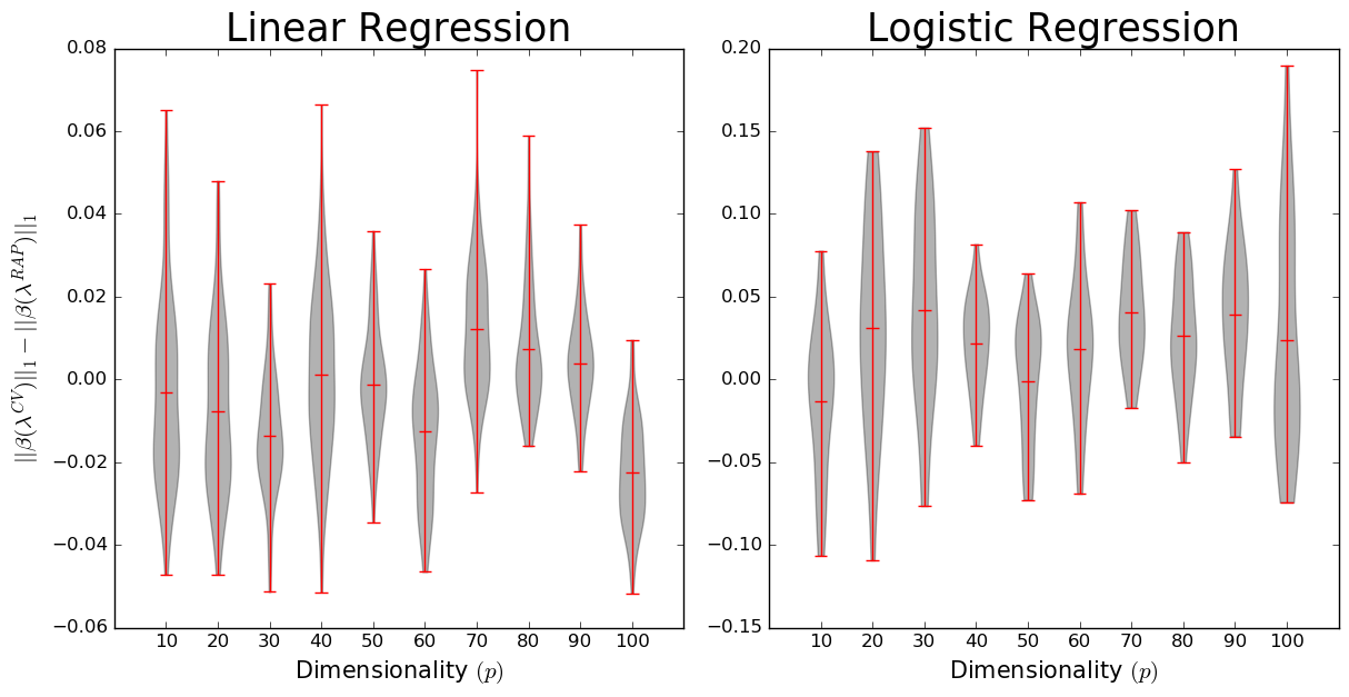
Figure 1: Violin plots visualizing the difference in selected regularization parameters as a function of the dimensionality, $p$, for linear (left) and logistic regression (right). We note that the difference in estimated $\ell_{1}$ norms is both small and centered around the origin, indicating the absence of large systematic bias. Note the difference in y-axis across panels.

The difference in selected regularization parameters over $N=500$ simulations is visualized in Figure 1. It is reassuring to note that, for both linear and logistic regression, the differences are both small in magnitude as well as centered around the origin. This serves to indicate the absence of a large systematic bias. However, we note that there is higher variance in the context of logistic regression.

5.4 Non-stationary data

While Section 5.3 provided empirical evidence demonstrating that the RAP framework can be effectively employed to track regularization parameters in a stationary setting, we are ultimately interested in streaming, non-stationary datasets. As a result, in this simulation we study the performance of the proposed framework in the context of non-stationary data. As in Section 5.3 we study the properties of the RAP algorithm in the context of linear and logistic regression.

While there are a multitude of methods through which to simulate non-stationary data, in this simulation study we chose to generate data with piece-wise stationary covariance structure. As a result, the underlying covariance alternated between two regimes: a sparse regime where the response was driven by a reduced subset of covariates and a dense regime where the converse was true. Thus, pairs $(y_{t},X_{t})$ of response and predictors were simulated in a piece-wise stationary regimes. The dimensionality of the covariates was fixed at $p=20$, implying that $X_{t}\in\mathbb{R}^{20}$. Changes occurred abruptly every 100 observations and two change-points were considered, resulting in $300$ observations in total.

Covariates, $X_{t}$, were simulated as described in Section 5.1 within two alternating regimes; dense and sparse. The block-covariance structure remained fix within each regime (i.e., for 100 observations). Within the dense regime, a proportion $\rho_{1}=0.8$ of regression coefficients were randomly selected and their values sampled from a standard Gaussian distribution. All remaining coefficients were set to zero. Similarly, in the case of the sparse regime, $\rho_{2}=0.2$ regression coefficients were randomly selected with remaining coefficients set to zero. The regression coefficients remained fixed within each regime.

In order to benchmark the performance of the proposed RAP framework, streaming penalized Lasso models were also estimated using a fixed and stepwise constant sparsity parameters. As a result, the RAP algorithm was benchmarked against three distinct offline methods for selecting the regularization parameter. In the case of a fixed sparsity parameter, $K=10$ fold cross-validation as well as Bayesian optimization were employed. Finally, cross-validation was also employed to learn a stepwise constant regularization parameter. This was achieved by performing cross-validation for the data within each regime. For each of these methods, their offline nature dictated that the entire dataset should be analyzed simultaneously (as opposed to in a streaming fashion by the RAP algorithm). As such, they serve to provide a benchmark but would infeasible in the context of streaming data.

Results for $N=500$ simulations are shown in Figure 2. The estimated time-varying regularization parameter for both the linear and logistic regression models is shown on the left panels. These results provide evidence that the RAP algorithm is able to reliably track the piece-wise constant regularization parameters selected by cross-validation. As expected, there is some lag directly after each change occurs, however, the estimated regression parameters is able to adapt thereafter. Figure 2 also shows the mean negative log-likelihood over unseen samples, $C_{t+1}$. We note there are abrupt spikes every 100 observations, corresponding to the abrupt changes in the underlying dependence structure. Detailed results are provided in Table 1. We note that the proposed framework is able to outperform the alternative offline approaches. In the case of the offline cross-validation and SMBO, this is to be expected as a fixed choice of regularization parameter is misspecified.

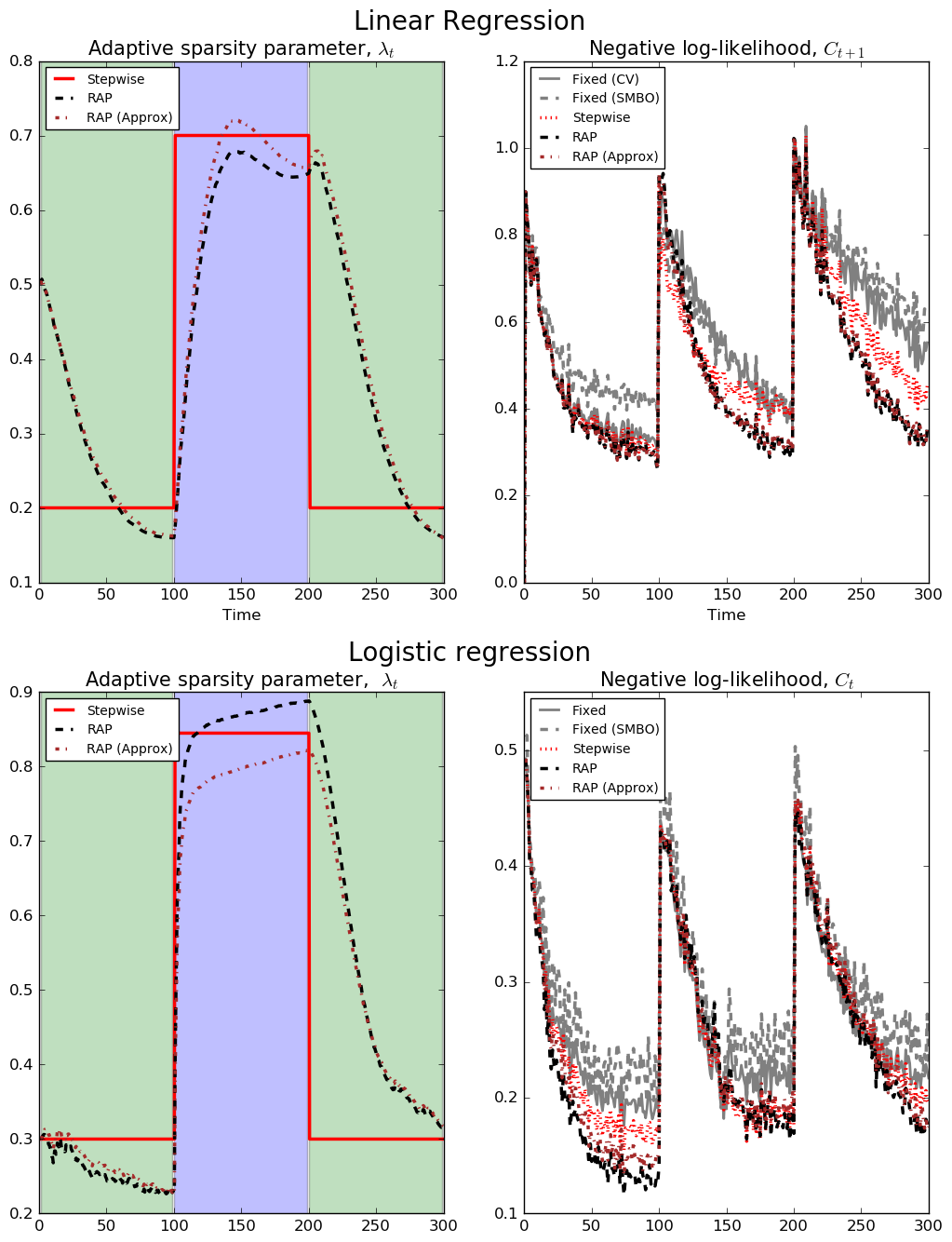
Figure 2: Simulation results when estimating regularized streaming linear and logistic regression models. Results for linear and logistic regression are shown across the first and second rows respectively. The left panels plot the mean regularization parameter as estimated by the RAP algorithm as well as the optimal piece-wise constant value selected via cross-validation. The right panels plot the mean negative log-likelihood, $C_{t+1}$, over time. We note that the RAP algorithms outperform the offline alternatives.

Table 1: Detailed results for simulation involving non-stationary data over $N=500$ independent iterations. We report the mean negative log-likelihood, $\bar{C}_{t}$, as well as the mean $F$-score, $\bar{F}_{t}$. Standard errors are provided in brackets.

	Linear regression		Logistic regression
Algorithm	A $\bar{C}_{t}$	$\bar{F}_{t}$	$\bar{C}_{t}$	$\bar{F}_{t}$
Fixed (CV)	0.58 (0.05)	0.49 (0.05)	0.25 (0.07)	0.49 (0.04)
Fixed (SMBO)	0.63 (0.05)	0.50 (0.07)	0.26 (0.08)	0.49 (0.05)
Stepwise	0.51 (0.04)	0.56 (0.04)	0.21 (0.06)	0.53 (0.04)
RAP	0.47 (0.04)	0.64 (0.06)	0.19 (0.04)	0.58 (0.03)
RAP (Approx)	0.48 (0.05)	0.63 (0.07)	0.20 (0.04)	0.55 (0.05)

6 Application to fMRI data

In this section we present an application of the RAP algorithm to task-based functional MRI (fMRI) data. This data corresponds to time-series measurements of blood oxygenation, a proxy for neuronal activity, taken across a set of spatially remote brain regions. Our objective in this work is to quantify pairwise statistical dependencies across brain regions, typically referred to as functional connectivity within the neuroimaging literature (Smith et al., 2011).

While traditional analysis of functional connectivity was rooted on the assumption of stationarity, there is growing evidence to suggest this is not the case (Hutchison et al., 2013). This particularly true in the context of task-based fMRI studies. Several methodologies have been proposed to address the non-stationary nature of fMRI data (Monti et al., 2014), many of which are premised on the use of penalized regression models such as those studied in this work. While such methods have made important progress in the study of non-stationary connectivity networks, they have typically employed fixed regularization parameters. This is difficult to justify in the context of non-stationary data and plausible biological justifications are not readily available. The RAP algorithm is therefore ideally suited to both accurately estimating non-stationary connectivity structure as well as providing insight regarding whether the assumption of a fixed sparsity parameter is reasonable.

6.1 Estimating connectivity via Lasso regressions

Estimating functional connectivity networks is fundamentally a statistical challenge. A functional relationship is said to exist across two spatially remote brain regions if their corresponding time-series share some statistical dependence. While this can be quantified in a variety of ways, a popular approach is the use of Lasso regression models to infer the conditional independence structure of a particular node. In such an approach, the time-series of a given node is regressed against the time-series of all remaining nodes. A functional relationship is subsequently inferred between the target node and all remaining nodes associated with a non-zero regression coefficient. The connectivity structure across all nodes can then be inferred via a neighborhood selection approach (Meinshausen and Bühlmann, 2006). The proposed RAP framework can directly be incorporated into such a model, resulting in time-varying conditional dependence structure where the underlying sparsity parameter is also inferred.

6.2 HCP Emotion Task Data

Emotion task data from the Human Connectome Project (HCP) was studied with 20 subjects selected at random. During the task participants were presented with blocks of trials that either required them to decide which of two faces presented on the bottom of the screen match the face at the top of the screen, or which of two shapes presented at the bottom of the screen match the shape at the top of the screen. The faces had either an angry or fearful expression while the shapes represented the emotionally neutral condition. Twenty regions were selected from an initial subset of 84 brain regions based on the Desikan-Killiany atlas. Data for each subject therefore consisted of $n=175$ observations across $p=20$ nodes.

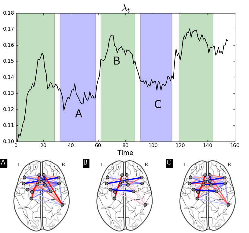
Figure 3: Top: the mean sparsity parameter is shown as a function of time. The background color indicates the nature of the task at hand (green indicates neutral task while blue indicates the emotion task). Bottom: estimated networks visualizing the estimated connectivity structure at three distinct points in time. Edge colors indicate the nature of the dependence (blue indicates a positive dependence, red a negative dependence).

6.3 Results

Data for each subject was analyzed independently where the time-varying estimates of the conditional dependence structure for each node were estimated as described in Section 6.1. A fixed forgetting factor of $r=.95$ was employed throughout with a stepsize parameter $\epsilon=.025$. The exact gradient was employed when updating the sparsity parameter at each iteration.

The mean sparsity parameter over all subjects is shown in the top panel of Figure 3. We observe decreased sparsity parameters for blocks in which subjects were presented with emotional (i.e., angry or fearful) faces (top panel, purple shaded areas) as compared to blocks in which subjects were shown neutral shapes (top panel, green shaded areas). The oscillation in sparsity parameter is highly correlated with task onset. When inspecting the networks estimated using the time varying sparsity parameter (bottom panel), we find strong coupling amongst many of the regions during the emotion processing blocks (A and C) compared to a clearly sparser network representation for blocks that require no emotion processing (i.e., neutral shapes, block B). This is to be expected as the selected regions are core hubs involved with emotion processing; therefore explaining the higher network activity during the emotion task.

7 Conclusion

In this work we have presented a framework through which to learn time-varying regularization parameters in the context of streaming generalized linear models. An approximate algorithm is also provided to address issues concerning computational efficiency. We present two simulation studies which demonstrate the capabilities of the RAP framework. These simulations show that the proposed framework is capable of tracking the regularization parameter both in a stationary as well as non-stationary setting. Finally, we present an application to task-based fMRI data, which is widely accepted to be non-stationary (Hutchison et al., 2013).

Future work will involve extending the RAP framework to consider alternative regularization schemes. In particular an $\ell_{2}$ penalty could also be incorporated as the derivative, $\frac{\partial\hat{\beta}_{t}(\lambda)}{\partial\lambda}$, is available in closed form.

Finally, the methods presented in this manuscript have been motivated by the study of fMRI data in real-time (Monti et al., 2017a). Future work will look to extend the proposed methodology, for example by combining with current approaches which involve graph embeddings (Monti et al., 2017b) or novel applications of real-time fMRI such as those described by Lorenz et al. (2016) and Lorenz et al. (2017). Another exciting avenue would be to use the proposed methods to understand variability in dynamic functional connectivity (Monti et al., 2015). Furthermore, it would also be interesting to consider alternative applications such as cyber-security (Gibberd et al., 2016), gene expression data (Gibberd and Nelson, 2017) and finance.

Appendix A Proof of Proposition 2

For a given regularization parameter, $\lambda$, the corresponding vector of estimated regression coefficients, $\hat{\beta}(\lambda)$, can be computed by minimizing the non-smooth objective, $L_{t}(\beta,\lambda)$, provided in equation (17). The sub-gradient is defined as:

$$\nabla_{\beta}L_{t}(\beta,\lambda)=-X_{1:t}^{T}W(y_{1:t}-\bm{\mu})\frac{\partial\bm{\eta}}{\partial\bm{\mu}}+\lambda~{}\mbox{sign}(\beta)$$ (20)

We write $\bm{\mu}$ to denote the vector of predicted means, $\mu_{i}=g^{-1}(\eta_{i})=g^{-1}(X_{i}^{T}\beta)$ and $\frac{\partial\bm{\eta}}{\partial\bm{\mu}}$ to denote a vector with entries $\frac{\partial{\eta}_{i}}{\partial{\mu}_{i}}$. Note that in the case of normal linear regression we have that $\mu_{i}=\eta_{i}=X_{i}^{T}\beta$ and we therefore recover equation (9).

As in Proposition 1, we have that for any choice of regularization parameter, the sub-gradient evaluated at $\hat{\beta}_{t}(\lambda)$ must satisfy:

$$\left.\nabla_{\beta}L_{t}(\beta,\lambda)\right|_{\beta=\hat{\beta}_{t}(\lambda)}\ni 0.$$

We therefore compute the derivative with respect to $\lambda$ in order to obtain:

$$\frac{\partial}{\partial\lambda}\left(\left.\nabla_{\beta}L_{t}(\beta,\lambda)\right|_{\beta=\hat{\beta}_{t}(\lambda)}\right) =0$$ (21)

$$=\frac{\partial}{\partial\lambda}\left(-X_{1:t}^{T}W(y_{1:t}-\bm{\mu})\frac{\partial\bm{\eta}}{\partial\bm{\mu}}\right)+\mbox{sign}(\hat{\beta}_{t}(\lambda))$$ (22)

$$=X_{1:t}^{T}W\frac{\partial\bm{\mu}}{\partial\lambda}\frac{\partial\bm{\eta}}{\partial\bm{\mu}}+\mbox{sign}(\hat{\beta}_{t}(\lambda))$$ (23)

$$=X_{1:t}^{T}WX_{1:t}\frac{\partial\hat{\beta}_{t}(\lambda)}{\partial\lambda}+\mbox{sign}(\hat{\beta}_{t}(\lambda))$$ (24)

where equation (24) follows from the fact that:

$$\frac{\partial\bm{\mu}}{\partial\lambda}=\frac{\partial\bm{\mu}}{\partial\bm{\eta}}\frac{\partial\bm{\eta}}{\partial\hat{\beta}_{t}(\lambda)}\frac{\partial\hat{\beta}_{t}(\lambda)}{\partial\lambda}=\frac{\partial\bm{\mu}}{\partial\bm{\eta}}X_{1:t}\frac{\partial\hat{\beta}_{t}(\lambda)}{\partial\lambda}.$$

Rearranging equation (24) yields the result.

References

- Aggarwal [2007] C. Aggarwal. Data streams: models and algorithms, volume 31. Springer Science & Business Media, 2007.
- Bottou [1998] L. Bottou. Online learning and stochastic approximations. On-line learning in neural networks, 17(9):142, 1998.
- Bottou [2010] L. Bottou. Large-scale machine learning with stochastic gradient descent. In COMPSTAT’2010, pages 177–186. Springer, 2010.
- Duchi et al. [2011] J. Duchi, E. Hazan, and Y. Singer. Adaptive subgradient methods for online learning and stochastic optimization. The Journal of Machine Learning Research, 12:2121–2159, 2011.
- Efron et al. [2004] B. Efron, T. Hastie, I. Johnstone, and R. Tibshirani. Least angle regression. The Annals of statistics, 32(2):407–499, 2004.
- Friedman et al. [2010] J. Friedman, T. Hastie, and R. Tibshirani. Regularization paths for generalized linear models via coordinate descent. Journal of statistical software, 33(1):1, 2010.
- Garrigues and Ghaoui [2009] P. Garrigues and L. Ghaoui. An homotopy algorithm for the lasso with online observations. In Advances in neural information processing systems, pages 489–496, 2009.
- Gibberd and Nelson [2014] A. Gibberd and J. Nelson. High dimensional changepoint detection with a dynamic graphical lasso. In Acoustics, Speech and Signal Processing (ICASSP), 2014 IEEE International Conference on, pages 2684–2688. IEEE, 2014.
- Gibberd and Nelson [2017] A. Gibberd and J. Nelson. Regularized estimation of piecewise constant gaussian graphical models: The group-fused graphical lasso. Journal of Computational and Graphical Statistics, (In Press), 2017.
- Gibberd et al. [2016] A. Gibberd, M. Evangelou, and J. Nelson. The time-varying dependency patterns of netflow statistics. In Data Mining Workshops (ICDMW), 2016 IEEE 16th International Conference on, pages 288–294. IEEE, 2016.
- Hastie et al. [2015] T. Hastie, R. Tibshirani, and M. Wainwright. Statistical learning with sparsity: the lasso and generalizations. CRC Press, 2015.
- Haykin [2008] S. Haykin. Adaptive filter theory. Pearson, 2008.
- Heard et al. [2010] N. Heard, D. Weston, K. Platanioti, and D. Hand. Bayesian anomaly detection methods for social networks. The Annals of Applied Statistics, 4(2):645–662, 2010.
- Hutchison et al. [2013] M. Hutchison, T. Womelsdorf, E. Allen, P. Bandettini, V. Calhoun, M. Corbetta, S. Della Penna, Jeff H Duyn, Gary H Glover, Javier Gonzalez-Castillo, et al. Dynamic functional connectivity: promise, issues, and interpretations. NeuroImage, 80:360–378, 2013.
- Lorenz et al. [2016] R. Lorenz, R. P. Monti, I. Violante, C. Anagnostopoulos, A. Faisal, G. Montana, and R. Leech. The automatic neuroscientist: a framework for optimizing experimental design with closed-loop real-time fMRI. NeuroImage, 129:320–334, 2016.
- Lorenz et al. [2017] R. Lorenz, A. Hampshire, and R. Leech. Neuroadaptive bayesian optimization and hypothesis testing. Trends in Cognitive Sciences, 2017.
- McCullagh and Nelder [1989] P. McCullagh and J. Nelder. Generalized linear models, volume 37. CRC press, 1989.
- McWilliams et al. [2014] B. McWilliams, C. Heinze, N. Meinshausen, G. Krummenacher, and H. Vanchinathan. LOCO: Distributing ridge regression with random projections. arXiv preprint arXiv:1406.3469, 2014.
- Meinshausen and Bühlmann [2006] N. Meinshausen and P. Bühlmann. High-dimensional graphs and variable selection with the lasso. The Annals of Statistics, pages 1436–1462, 2006.
- Meinshausen and Bühlmann [2010] N. Meinshausen and P. Bühlmann. Stability selection. Journal of the Royal Statistical Society: Series B, 72(4):417–473, 2010.
- Monti et al. [2014] R. P. Monti, P. Hellyer, D. Sharp, R. Leech, C. Anagnostopoulos, and G. Montana. Estimating time-varying brain connectivity networks from functional MRI time series. NeuroImage, 103:427–443, 2014.
- Monti et al. [2015] R. P. Monti, C. Anagnostopoulos, and G. Montana. Learning population and subject-specific brain connectivity networks via mixed neighborhood selection. arXiv preprint arXiv:1512.01947, 2015.
- Monti et al. [2017a] R. P. Monti, R. Lorenz, R. Braga, C. Anagnostopoulos, R. Leech, and G. Montana. Real-time estimation of dynamic functional connectivity networks. Human brain mapping, 38(1):202–220, 2017a.
- Monti et al. [2017b] R. P. Monti, R. Lorenz, P. Hellyer, R. Leech, C. Anagnostopoulos, and G. Montana. Decoding time-varying functional connectivity networks via linear graph embedding methods. Frontiers in computational neuroscience, 11, 2017b.
- Park and Hastie [2007] M. Park and T. Hastie. L1-regularization path algorithm for generalized linear models. Journal of the Royal Statistical Society: Series B (Statistical Methodology), 69(4):659–677, 2007.
- Rosset and Zhu [2007] S. Rosset and J. Zhu. Piecewise linear regularized solution paths. The Annals of Statistics, pages 1012–1030, 2007.
- Shahriari et al. [2016] B. Shahriari, K. Swersky, Z. Wang, R. Adams, and N. de Freitas. Taking the human out of the loop: A review of bayesian optimization. IEEE Proceedings, 104(1):148–175, 2016.
- Smith et al. [2011] S. Smith, K. Miller, G. Salimi-Khorshidi, M. Webster, C. Beckmann, T. Nichols, J. Ramsey, and M. Woolrich. Network modelling methods for fMRI. NeuroImage, 54(2):875–891, 2011.
- Tibshirani [1996] R. Tibshirani. Regression shrinkage and selection via the lasso. Journal of the Royal Statistical Society. Series B, pages 267–288, 1996.
- Tibshirani [2013] R. Tibshirani. The lasso problem and uniqueness. Electronic Journal of Statistics, 7:1456–1490, 2013.
- Weiskopf [2012] N. Weiskopf. Real-time fMRI and its application to neurofeedback. NeuroImage, 62(2):682–692, 2012.