Temperatures are not useful to characterise bright-soliton experiments for ultra-cold atoms
Abstract
Contrary to many other translationally invariant one-dimensional models, the low-temperature phase for an attractively interacting one-dimensional Bose-gas (a quantum bright soliton) is stable against thermal fluctuations. However, treating the thermal properties of quantum bright solitons within the canonical ensemble leads to anomalous fluctuations of the total energy that indicate that canonical and micro-canonical ensembles are not equivalent. State-of-the-art experiments are best described by the micro-canonical ensemble, within which we predict a co-existence between single atoms and solitons even in the thermodynamic limit — contrary to strong predictions based on both the Landau hypothesis and the canonical ensemble. This questions the use of temperatures to describe state-of-the-art bright soliton experiments that currently load Bose-Einstein condensates into quasi-one-dimensional wave guides without adding contact to a heat bath.
pacs:
03.75.Lm, 05.45.Yv, 67.85.BcThe experimental realization Meyrath et al. (2005); Gaunt et al. (2013) of a box potential opens new doors in investigating translationally invariant systems of ultra-cold atoms. For ideal gases in one-dimension there is no Bose-Einstein condensate (BEC), whereas the presence of a harmonic trap leads to a quasi-condensate Herzog and Olshanii (1997). For attractively interacting Bose gases, the ground state is a weakly bound molecule, a matter-wave bright soliton. Some of its properties are remarkably different from those of BECs: as we will see below, there is no off-diagonal long-range order. Thus, mathematical theorems about the non-existence Mermin and Wagner (1966); Hohenberg (1967) of off-diagonal long-range order do not lead to additional physical insight for this model system.
Matter-wave bright solitons have been experimentally generated for ultracold atomic gases in quasi-one-dimensional wave guides for attractive interactions Khaykovich et al. (2002); Strecker et al. (2002); Cornish et al. (2006); Marchant et al. (2013); Medley et al. (2014); McDonald et al. (2014); Nguyen et al. (2014); Everitt et al. (2015); Marchant et al. (2016); Lepoutre et al. (2016) and, in the presence of an optical lattice, also for repulsive interactions Eiermann et al. (2004). For dark solitons Burger et al. (1999), developing a complete understanding by modeling them on the many-particle quantum level Girardeau and Wright (2000); Mishmash and Carr (2009); Delande and Sacha (2014); Krönke and Schmelcher (2015); Karpiuk et al. (2015); Syrwid and Sacha (2015) is crucial. The same is true for bright solitons. We note that quasi-one-dimensional wave guides provide thermalisation mechanisms Mazets and Schmiedmayer (2010).
When modeling the statistical physics, experiments with ultra-cold atoms arguably are best described by the micro-canonical ensemble (MCE, with fixed total energy and fixed particle number Pathria and Beale (2011)). As long as the different ensembles are equivalent one can choose a simpler ensemble, such as the canonical ensemble (CE, which allows the energy to fluctuate; while the particle number still is fixed, we now have the temperature as a thermodynamic variable Pathria and Beale (2011)). For attractive bosons in a quasi-one-dimensional wave guide the canonical ensemble even predicts that the thermal weakly-bound molecule–non-molecule crossover becomes a phase transition in the thermodynamic limit Herzog et al. (2014); Weiss (2016). However, as we will see, the energy fluctuations are anomalously large, making it necessary to re-investigate the transition on the level of the micro-canonical ensemble. Furthermore, this implies that while the canonical ensemble is a powerful tool to describe both the high- and low-temperature phases Herzog et al. (2014); Weiss (2016), it fails to capture the physics of the crossover itself correctly for thermally isolated systems with ultracold atoms.
For attractively interacting atoms () in one dimension, the integrable Lieb-Liniger-(McGuire) Hamiltonian Lieb and Liniger (1963); McGuire (1964) is a very useful model
| (1) |
where denotes the position of particle of mass , and the interaction strength
| (2) |
is set by the s-wave scattering length and the perpendicular angular trapping-frequency Olshanii (1998). For sufficiently large foo we have the ground state energy McGuire (1964)
| (3) |
and all excited energies Castin and Herzog (2001)
| (4) |
corresponding to the intuitive picture of solitonlets of size and their respective center-of-mass kinetic energies.
The ground state wave function
| (5) |
is translationally invariant and corresponds to a quantum bright soliton — a weakly bound molecule with delocalized center-of-mass wave function and localized relative wave function. It also helps to quantify what a sufficiently large is foo . The size of the molecule can also be characterized by the single particle density (after replacing the delocalized center-of-mass wave function by a delta function at Calogero and Degasperis (1975); Castin and Herzog (2001), which is identical to the mean-field result Pethick and Smith (2008))
| (6) |
In order to ensure that a finite-temperature phase transition does not violate the (Hohenberg)-Mermin-Wagner theorem Mermin and Wagner (1966); Hohenberg (1967), we use the thermodynamic limit Herzog et al. (2014); Weiss (2016)
| (7) |
where the particle number , system length , interaction strength and soliton length are defined in Eqs. (1), (2) and (6).
We note that there is no off-diagonal long-range order111There is, however, long-range order in the limit investigated in addition to the limit (7) in Ref. Herzog et al. (2014). Thus, given the (Hohenberg-)Mermin-Wagner theorem Mermin and Wagner (1966); Hohenberg (1967) one should expect the characteristic temperature to approach zero for the infinite system. This is indeed the case Cas (2014). for bright solitons in the limit (7). The many-particle ground state can be viewed as consisting of a relative222The wave-function described in terms of the relative motional degrees of freedom — which we call the relative wave-function. wave-function given by a Hartree product state with particles occupying the mean-field-bright-soliton mode [see Eq. (6)]; and a center-of-mass wave function for the variable (cf. Calogero and Degasperis (1975); Castin and Herzog (2001)). The one-body density matrix Pitaevskii and Stringari (2003) then is which vanishes in the limit even after integrating over . Thus, there is no off-diagonal long range order in our system Weiss (2016); the existence of bright solitons at low but non-zero temperatures in the thermodynamic limit (7) therefore does not violate the (Hohenberg-)Mermin-Wagner theorem Mermin and Wagner (1966); Hohenberg (1967).
However, there is a severe problem with the canonical description of the attractive Lieb-Liniger gas in 1D: the scaling of the specific heat Weiss (2016). The average energy changes sign at the transition temperature from a negative value (3) — which scales in the limit (7) — to a positive value within a temperature range . By using the textbook results for calculating the specific heat Pathria and Beale (2011) we thus obtain
| (8) |
near the transition temperature. Ensemble equivalence between MCE and CE would usually require a scaling not faster than (rather than ) — as is the case outside the transition region Weiss (2016). Thus a complete description will require a micro-canonical treatment with fixed total energy (possibly including some very small energy uncertainty) within the MCE, which is the most suitable ensemble for state-of-the-art bright soliton experiments Khaykovich et al. (2002); Strecker et al. (2002); Cornish et al. (2006); Marchant et al. (2013); Medley et al. (2014); McDonald et al. (2014); Nguyen et al. (2014); Everitt et al. (2015); Marchant et al. (2016); Lepoutre et al. (2016). Nevertheless we can profit from the CE result as we know what happens both at high temperatures ( single atoms) and at low temperatures (a single bright soliton containing all atoms) Herzog et al. (2014); Weiss (2016). We only have to identify the energy regimes which correspond to these two phases. Note that the disagreement between MCE and CE only happens in the transition region of size which vanishes in the limit (7) and thus appears to be negligible for practical purposes. However, as we will see below, this region covers a huge energy scale and covers all experimentally accessible cases of realising bright solitons in a one-dimensional wave guide — as long as 3D effects can be discarded.
For very low total energies [], when approaching the internal ground state energy [], only the internal ground state (plus some non-degenerate kinetic energy of the big soliton) is energetically accessible — as long as
For slightly higher (less negative) total energy, the only energetically accessible states are the -particle soliton or, alternatively, an -particle soliton and a single unbound particle. Naively applying the Landau hypothesis333According to the textbook series by Landau and Lifshitz (the very end of Ref. Lifshitz and Pitaevskii (2002)), the co-existence of single unbound atoms with one bound state or several bound states is excluded in a large class of 1D systems. suggests that it must be the former as the only “allowed” options seem to be either the single atoms or an -particle soliton. However, when counting possible configurations the -particle soliton will always lose compared to distributing the kinetic energy among two or more smaller solitons or solitons and single particles.
We hasten to add that there is of course no error in the derivation of the Landau hypothesis (footnote 3; page 3) as given in what is frequently considered to be an authoritative text on theoretical physics Lifshitz and Pitaevskii (2002). However, its powerful statement is based on assumptions that, while fulfilled by a huge class of models, are not fulfilled by the attractive Lieb-Liniger model. One example is that the size of many objects scales with the number of particles the object is composed of; like neutron stars, bright solitons become smaller with larger particle numbers [Eq. (6)].
Here, as long as the total energy is negative, , within the MCE the configuration consisting of single atoms is simply not energetically accessible (the single atom case has a positive total energy) and the configuration of an -atom soliton is in most cases statistically irrelevant. A summary of the three energy regimes can be found in Table 1.
| regime | |||
|---|---|---|---|
| MCE | atoms | coexistence | one large soliton |
In order to gain a better understanding of what would happen in an experiment within the co-existence region
| (9) |
we will distribute a negative energy that is proportional to the ground state energy:
| (10) |
The number of possibilities to distribute atoms among up to solitonlets for the distinct energy eigenstates (4) is given by the number partitioning problem which asymptotically reads Abramowitz and Stegun (1984)
| (11) |
When there is no kinetic energy, all energies of the type given in Eq. (4) lie between 0 and the ground-state energy as for . Thus, for typical energies distributing all particles into all possible solitonlets would give an exponentially growing number of states (11) — but this grows only to the power and as we show below is thus not the leading order contribution.
So far, the above considerations ignore distribution of the kinetic energy. For single atoms and large enough kinetic energy , the accessible number of states scales as for the classical gas. We note that quantum corrections are negligible as there is no condensation temperature for non-interacting Bose-gases in a one-dimensional translationally invariant wave-guide. Thus, all possible quantum corrections must vanish in the limit (7) because the transition temperature remains finite in the canonical calculations Herzog et al. (2014); Weiss (2016). Hence, the leading contribution to the total number of configurations reads Pathria and Beale (2011)
| (12) |
If is (at least) extensive (), this thus grows considerably faster with than the number partitioning problem (11).
Outside the crossover region there are no differences between the canonical and micro-canonical ensemble [see text below Eq. (8)], thus we can use the canonical predictions as a basis for our micro-canonical calculations. This confirms that the most probable outcome consists of solitonlets of size at high enough total energies. For positive total energies, all particles can be in such a state. However, for negative total energies this is no longer the case.
The large exponential growth (12) clearly suggests that we should have as many single atoms as possible. Thus, the negative total energy should be carried by one large soliton and there should be many solitonlets of unit size carrying kinetic energy:
It would of course be possible to increase the kinetic energy by adding a further larger solitonlet and reducing the number of single unbound atoms. But the scaling of Eq. (12) and the canonical treatment of the high-temperature phase Herzog et al. (2014); Weiss (2016) clearly shows that these configurations are not statistically relevant. Thus, the leading contribution to the number of possible configurations is
| (13) |
Taking the leading order approximation ,
| (14) |
and then using
| (15) |
we can show that is indeed small for negative . With the “maximum finding condition”
then implies in leading order
In the limit (7) and for , is independent of (as is ). All other quantities (including ) are proportional to . This yields the leading-order behaviour map
| (16) |
in the limit (7) where and are constants. The Lambert function solves the equation .
Repeating the above calculation for we have as our starting point
| (17) |
and we have again that in the limit (7).
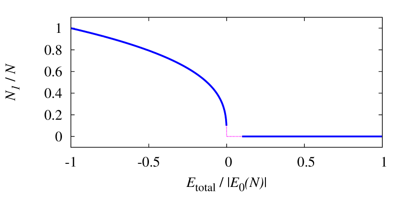
Figure 1 shows the size of the largest soliton as predicted by the MCE. Parameters near are consistent with soliton trains Hai et al. (2004); Carr and Brand (2004); Streltsov et al. (2011) which were observed in the experiment of Ref. Strecker et al. (2002): for, say, five solitons of equal size, the total ground state energy would be only of (in the absence of kinetic energy).
To conclude, the statistical ensembles MCE and CE are not equivalent for the Lieb-Liniger model with attractive interactions. The violation of ensemble equivalence is indicated by anomalous (canonical) energy fluctuations. We note that the existence of anomalous fluctuations — that have been discussed for condensate fluctuations Svidzinsky and Scully (2006); Gajda and Rza¸żewski (1997); Hauge (1970), both for non-interacting Bose-Einstein condensates Weiss and Wilkens (1997); Grossmann and Holthaus (1997); Idziaszek et al. (1999) and for interacting models Giorgini et al. (1998); Meier and Zwerger (2001) — has been questioned for interacting equilibrium systems Yukalov (2005a, b).
The Landau hypothesis suggests that a large soliton and single unbound atoms cannot co-exist. While this is valid in the CE Herzog et al. (2014); Weiss (2016), in the MCE co-existence takes place — the assumptions on which the Landau hypothesis is based are valid for many models but not the Lieb-Liniger model with attractive interactions. This is not the only curious property of the translationally invariant attractive Lieb-Liniger model: it is one of the examples for which a 1D finite-temperatures phase transition exists Herzog et al. (2014); Weiss (2016); another example can be found in Ref. Aleiner et al. (2010).
As state-of-the-art experiments arguably are best described by an isolated system without contact to a heat bath, neither anomalous nor normal energy fluctuations occur — but co-existence of the two phases does. Using a temperature to describe bright solitons would require a heat bath and is thus questionable for state-of-the-art bright soliton experiments in BECs Khaykovich et al. (2002); Strecker et al. (2002); Cornish et al. (2006); Marchant et al. (2013); Medley et al. (2014); McDonald et al. (2014); Nguyen et al. (2014); Everitt et al. (2015); Marchant et al. (2016); Lepoutre et al. (2016). Given that the temperature barely changes over the energy regime relevant for the existence of bright solitons, it seems to be easier to simply approximately give it as the transition temperature Weiss (2016); Herzog et al. (2014) and calculate it for the experimentally relevant parameters, the result being practically identical for 73% of all particles occupying one large soliton or, say, 42%. As the corresponding energy difference is rather large, getting from one to the other requires more experimental effort than the tiny temperature difference might suggest. This behaviour is similar to water freezing or ice melting without any change of temperature. For bright solitons in the presence of a harmonic trap, classical field theory has been used to investigate the statistics of an attractive 1D Bose gas Bienias et al. (2011), an approach that might help to investigate the open question about the statistics near .
The data presented in this paper are available online Weiss et al. (2016).
Acknowledgements.
We thank T. P. Billam, L. D. Carr, Y. Castin, J. Tempere and T. P. Wiles for discussions. C.W. and S.A.G. thank the UK Engineering and Physical Sciences Research Council (Grant No. EP/L010844/1) for funding. B.G. thanks the European Union for funding through FP7-PEOPLE-2013-IRSES Grant Number 605096.References
- Meyrath et al. (2005) T. P. Meyrath, F. Schreck, J. L. Hanssen, C.-S. Chuu, and M. G. Raizen, “Bose-Einstein condensate in a box,” Phys. Rev. A 71, 041604 (2005).
- Gaunt et al. (2013) A. L. Gaunt, T. F. Schmidutz, I. Gotlibovych, R. P. Smith, and Z. Hadzibabic, “Bose-Einstein condensation of atoms in a uniform potential,” Phys. Rev. Lett. 110, 200406 (2013).
- Herzog and Olshanii (1997) C. Herzog and M. Olshanii, “Trapped bose gas: The canonical versus grand canonical statistics,” Phys. Rev. A 55, 3254 (1997).
- Mermin and Wagner (1966) N. D. Mermin and H. Wagner, “Absence of ferromagnetism or antiferromagnetism in one- or two-dimensional isotropic Heisenberg models,” Phys. Rev. Lett. 17, 1133 (1966).
- Hohenberg (1967) P. C. Hohenberg, “Existence of long-range order in one and two dimensions,” Phys. Rev. 158, 383 (1967).
- Khaykovich et al. (2002) L. Khaykovich, F. Schreck, G. Ferrari, T. Bourdel, J. Cubizolles, L. D. Carr, Y. Castin, and C. Salomon, “Formation of a matter-wave bright soliton,” Science 296, 1290 (2002).
- Strecker et al. (2002) K. E. Strecker, G. B. Partridge, A. G. Truscott, and R. G. Hulet, “Formation and propagation of matter-wave soliton trains,” Nature (London) 417, 150 (2002).
- Cornish et al. (2006) S. L. Cornish, S. T. Thompson, and C. E. Wieman, “Formation of bright matter-wave solitons during the collapse of attractive Bose-Einstein condensates,” Phys. Rev. Lett. 96, 170401 (2006).
- Marchant et al. (2013) A. L. Marchant, T. P. Billam, T. P. Wiles, M. M. H. Yu, S. A. Gardiner, and S. L. Cornish, “Controlled formation and reflection of a bright solitary matter-wave,” Nat. Commun. 4, 1865 (2013).
- Medley et al. (2014) P. Medley, M. A. Minar, N. C. Cizek, D. Berryrieser, and M. A. Kasevich, “Evaporative production of bright atomic solitons,” Phys. Rev. Lett. 112, 060401 (2014).
- McDonald et al. (2014) G. D. McDonald, C. C. N. Kuhn, K. S. Hardman, S. Bennetts, P. J. Everitt, P. A. Altin, J. E. Debs, J. D. Close, and N. P. Robins, “Bright solitonic matter-wave interferometer,” Phys. Rev. Lett. 113, 013002 (2014).
- Nguyen et al. (2014) J. H. V. Nguyen, P. Dyke, D. Luo, B. A. Malomed, and R. G. Hulet, “Collisions of matter-wave solitons,” Nat. Phys. 10, 918 (2014).
- Everitt et al. (2015) P. J. Everitt, M. A. Sooriyabandara, G. D. McDonald, K. S. Hardman, C. Quinlivan, M. Perumbil, P. Wigley, J. E. Debs, J. D. Close, C. C. N. Kuhn, and N. P. Robins, “Observation of Breathers in an Attractive Bose Gas,” ArXiv e-prints (2015), arXiv:1509.06844 [cond-mat.quant-gas] .
- Marchant et al. (2016) A. L. Marchant, T. P. Billam, M. M. H. Yu, A. Rakonjac, J. L. Helm, J. Polo, C. Weiss, S. A. Gardiner, and S. L. Cornish, “Quantum reflection of bright solitary matter waves from a narrow attractive potential,” Phys. Rev. A 93, 021604(R) (2016).
- Lepoutre et al. (2016) S Lepoutre, L Fouché, A Boissé, G Berthet, G Salomon, A Aspect, and T Bourdel, “Production of strongly bound 39K bright solitons,” ArXiv e-prints (2016), arXiv:1609.01560 [physics.atom-ph] .
- Eiermann et al. (2004) B. Eiermann, Th. Anker, M. Albiez, M. Taglieber, P. Treutlein, K.-P. Marzlin, and M. K. Oberthaler, “Bright Bose-Einstein gap solitons of atoms with repulsive interaction,” Phys. Rev. Lett. 92, 230401 (2004).
- Burger et al. (1999) S. Burger, K. Bongs, S. Dettmer, W. Ertmer, K. Sengstock, A. Sanpera, G. V. Shlyapnikov, and M. Lewenstein, “Dark solitons in Bose-Einstein condensates,” Phys. Rev. Lett. 83, 5198 (1999).
- Girardeau and Wright (2000) M. D. Girardeau and E. M. Wright, “Dark solitons in a one-dimensional condensate of hard core bosons,” Phys. Rev. Lett. 84, 5691 (2000).
- Mishmash and Carr (2009) R. V. Mishmash and L. D. Carr, “Quantum entangled dark solitons formed by ultracold atoms in optical lattices,” Phys. Rev. Lett. 103, 140403 (2009).
- Delande and Sacha (2014) D. Delande and K. Sacha, “Many-body matter-wave dark soliton,” Phys. Rev. Lett. 112, 040402 (2014).
- Krönke and Schmelcher (2015) S. Krönke and P. Schmelcher, “Many-body processes in black and gray matter-wave solitons,” Phys. Rev. A 91, 053614 (2015).
- Karpiuk et al. (2015) T. Karpiuk, T. Sowiński, M. Gajda, K. Rzazewski, and M. Brewczyk, “Correspondence between dark solitons and the type II excitations of the Lieb-Liniger model,” Phys. Rev. A 91, 013621 (2015).
- Syrwid and Sacha (2015) A. Syrwid and K. Sacha, “Lieb-liniger model: Emergence of dark solitons in the course of measurements of particle positions,” Phys. Rev. A 92, 032110 (2015).
- Mazets and Schmiedmayer (2010) I E Mazets and J Schmiedmayer, “Thermalization in a quasi-one-dimensional ultracold bosonic gas,” New J. Phys. 12, 055023 (2010).
- Pathria and Beale (2011) R. K. Pathria and Paul D. Beale, Statistical Mechanics (Butterworth-Heinemann, Oxford, 2011).
- Herzog et al. (2014) C. Herzog, M. Olshanii, and Y. Castin, “Une transition liquide–gaz pour des bosons en interaction attractive à une dimension,” Comptes Rendus Physique 15, 285 (2014), arXiv:1311.3857 .
- Weiss (2016) C. Weiss, “Finite-temperature phase transition in a homogeneous one-dimensional gas of attractive bosons,” http://arxiv.org/a/weiss_c_1 (2016).
- Lieb and Liniger (1963) E. H. Lieb and W. Liniger, “Exact Analysis of an Interacting Bose Gas. I. The General Solution and the Ground State,” Phys. Rev. 130, 1605 (1963).
- McGuire (1964) J. B. McGuire, “Study of Exactly Soluble One-Dimensional N-Body Problems,” J. Math. Phys. 5, 622 (1964).
- Olshanii (1998) M. Olshanii, “Atomic scattering in the presence of an external confinement and a gas of impenetrable bosons,” Phys. Rev. Lett. 81, 938 (1998).
- (31) To define sufficiently large , we should look at the size of the relative wave function of a two-particle soliton [Eq. (5)], yielding: .
- Castin and Herzog (2001) Y. Castin and C. Herzog, “Bose-Einstein condensates in symmetry breaking states,” C. R. Acad. Sci. Paris, Ser. IV 2, 419 (2001), arXiv:cond-mat/0012040 .
- Calogero and Degasperis (1975) F. Calogero and A. Degasperis, “Comparison between the exact and Hartree solutions of a one-dimensional many-body problem,” Phys. Rev. A 11, 265 (1975).
- Pethick and Smith (2008) C. J. Pethick and H. Smith, Bose-Einstein Condensation in Dilute Gases (Cambridge University Press, Cambridge, 2008).
- Cas (2014) “Y. Castin. Private communication,” (2014).
- Pitaevskii and Stringari (2003) L. Pitaevskii and S. Stringari, Bose-Einstein Condensation (Clarendon Press, Oxford, 2003).
- Lifshitz and Pitaevskii (2002) E. M. Lifshitz and L. P. Pitaevskii, Landau and Lifshitz — Course of Theoretical Physics, Vol. 9: Statistical Physics, Part 1 (Butterworth-Heinemann, Oxford, 2002).
- Abramowitz and Stegun (1984) M. Abramowitz and I. A. Stegun, Pocketbook of Mathematical Functions (Verlag Harri Deutsch, Thun, 1984).
- (39) Computer algebra programme MAPLE, http://www.maplesoft.com/.
- Hai et al. (2004) W. Hai, C. Lee, and G. Chong, “Propagation and breathing of matter-wave-packet trains,” Phys. Rev. A 70, 053621 (2004).
- Carr and Brand (2004) L. D. Carr and J. Brand, “Spontaneous soliton formation and modulational instability in Bose-Einstein condensates,” Phys. Rev. Lett. 92, 040401 (2004).
- Streltsov et al. (2011) A. I. Streltsov, O. E. Alon, and L. S. Cederbaum, “Swift loss of coherence of soliton trains in attractive Bose-Einstein condensates,” Phys. Rev. Lett. 106, 240401 (2011).
- Svidzinsky and Scully (2006) A. A. Svidzinsky and M. O. Scully, “Condensation of n interacting bosons: A hybrid approach to condensate fluctuations,” Phys. Rev. Lett. 97, 190402 (2006).
- Gajda and Rza¸żewski (1997) M. Gajda and K. Rza¸żewski, “Fluctuations of Bose-Einstein condensate,” Phys. Rev. Lett. 78, 2686 (1997).
- Hauge (1970) E. H. Hauge, “Fluctuations in ground state occupation number of ideal Bose gas,” Physica Nor. 4, 19 (1970).
- Weiss and Wilkens (1997) C. Weiss and M. Wilkens, “Particle number counting statistics in ideal Bose gases,” Opt. Express 1, 272 (1997).
- Grossmann and Holthaus (1997) S. Grossmann and M. Holthaus, “Maxwell’s demon at work: Two types of Bose condensate fluctuations in power-law traps,” Opt. Express 1, 262 (1997).
- Idziaszek et al. (1999) Z. Idziaszek, M. Gajda, P. Navez, M. Wilkens, and K. Rza¸żewski, “Fluctuations of the weakly interacting Bose-Einstein condensate,” Phys. Rev. Lett. 82, 4376 (1999).
- Giorgini et al. (1998) S. Giorgini, L. P. Pitaevskii, and S. Stringari, “Anomalous fluctuations of the condensate in interacting Bose gases,” Phys. Rev. Lett. 80, 5040 (1998).
- Meier and Zwerger (2001) F. Meier and W. Zwerger, “Anomalous condensate fluctuations in strongly interacting superfluids,” Phys. Rev. A 64, 033610 (2001).
- Yukalov (2005a) V. I. Yukalov, “No anomalous fluctuations exist in stable equilibrium systems,” Phys. Lett. A 340, 369 (2005a).
- Yukalov (2005b) V. I. Yukalov, “Fluctuations of composite observables and stability of statistical systems,” Phys. Rev. E 72, 066119 (2005b).
- Aleiner et al. (2010) I. L. Aleiner, B. L. Altshuler, and G. V. Shlyapnikov, “A finite-temperature phase transition for disordered weakly interacting bosons in one dimension,” Nat. Phys. 6, 900 (2010).
- Bienias et al. (2011) P. Bienias, K. Pawlowski, M. Gajda, and K. Rzazewski, “Statistical properties of one-dimensional attractive Bose gas,” EPL (Europhys. Lett.) 96, 10011 (2011).
- Weiss et al. (2016) C. Weiss, S. A. Gardiner, and B. Gertjerenken, https://collections.durham.ac.uk/files/vt150j26r, http://dx.doi.org/10.15128/vt150j26r (2016), “Temperatures are not useful to characterise bright-soliton experiments for ultra-cold atoms: Supporting data”.