Finite-temperature phase transition in a homogeneous one-dimensional gas of attractive bosons

Abstract

In typical one-dimensional models the Mermin-Wagner theorem forbids long range order, thus preventing finite-temperature phase transitions. We find a finite-temperature phase transition for a homogeneous system of attractive bosons in one dimension. The low-temperature phase is characterized by a quantum bright soliton without long range order; the high-temperature phase is a free gas. Numerical calculations for finite particle numbers show a specific heat scaling as $N^{2}$, consistent with a vanishing transition region in the thermodynamic limit.

Bright solitons generated from attractively interacting Bose-Einstein condensates in quasi-one-dimensional wave guides are investigated experimentally in an increasing number of experimentsKhaykovich et al. (2002); Strecker et al. (2002); Cornish et al. (2006); Marchant et al. (2013); Medley et al. (2014); McDonald et al. (2014); Nguyen et al. (2014); Marchant et al. (2016); Everitt et al. (2015); Lepoutre et al. (2016). As experiments do not truly take place in one dimension but rather in quasi-one-dimensional wave guides, providing a thermalization mechanism Mazets and Schmiedmayer (2010); Cockburn et al. (2011), this leads to the question whether or not these bright solitons can be stable in the presence of thermal fluctuations.

The Mermin-Wagner theorem Mermin and Wagner (1966) proves that in many models long-range order in one or two dimensions cannot exist at finite temperatures Mermin and Wagner (1966); Hohenberg (1967); this excludes the existence of many phase transitions. Finite-temperature transitions are fundamentally different from quantum phase transitions (cf. Jaksch et al. (1998); Greiner et al. (2002)); one-dimensional quantum phase transitions can be found, e.g., in Refs. Zwerger (2003); Cincio et al. (2007); Kanamoto et al. (2010)). While there are some finite temperature phase transitions in low-dimensional systems like the Berezinsky-Kosterlitz-Thouless transition in two dimensions Hadzibabic et al. (2006) or the phase transition in the two-dimensional Ising model Onsager (1944), the generic case is that low-dimensional models to not undergo finite-temperature phase transitions Gelfert and Nolting (2001). Indeed, a book on “thermodynamics of one-dimensional solvable models” does not include the word “phase transition” in its index Takahashi (2005). For a disordered system displaying Anderson-localization Anderson (1958), a finite-temperature phase transition for weakly interacting bosons in one dimension has been found in Ref. Aleiner et al. (2010).

A quasi one-dimensional system of attractively interacting bosons can be modeled Lai and Haus (1989); Castin and Herzog (2001); Calabrese and Caux (2007); Muth and Fleischhauer (2010) by the solvable Lieb-Liniger model Lieb and Liniger (1963); McGuire (1964); Seiringer and Yin (2008). One of the challenges for bright-soliton experiments Khaykovich et al. (2002); Strecker et al. (2002); Cornish et al. (2006); Pollack et al. ; Marchant et al. (2013); Medley et al. (2014); McDonald et al. (2014); Nguyen et al. (2014) is to realize true quantum behavior predicted, so far, with zero-temperature calculations Carr and Brand (2004); Weiss and Castin (2009); Streltsov et al. (2009); Sacha et al. (2009); Streltsov et al. (2011); Gertjerenken et al. (2013); Barbiero and Salasnich (2014). For the Lieb-Liniger model, investigations of thermal effects on the many-body level for bosons in one dimension have so far focused on the more extensively studied case of repulsive interactions (Ref. Takahashi (2005) and references therein); for finite systems classical field methods have been applied Bienias et al. (2011). In other soliton models, thermodynamics with interacting solitons has been investigated Zabusky and Kruskal (1965); Currie et al. (1980).

In this Letter we show that attractive bosons in the Lieb-Liniger model undergo a finite-temperature phase transition; a bright soliton – no-soliton transition. As bright solitons do not display long-range order, this does not violate the Mermin-Wagner theorem. Although bright solitons do not display long-range order, quantum bright solitons are fundamentally different from localized states cf. Aleiner et al. (2010): For the Lieb-Liniger model, the energy eigenfunction describing a soliton of $N$-particles has to obey the symmetry of the Hamiltonian and is thus translationally invariant.

For $N$ identical bosons on a one-dimensional line of length $L$, corresponding to the experimentally realizable Schmidutz et al. (2014) box potential, the Lieb-Liniger Hamiltonian reads Lieb and Liniger (1963); McGuire (1964); Seiringer and Yin (2008)

$$\hat{H}= -\sum_{j=1}^{N}\frac{\hbar^{2}}{2m}\frac{\partial^{2}}{\partial{x_{j}}^{2}}+\sum_{j=1}^{N-1}\sum_{n=j+1}^{N}g_{1\rm D}\delta\left(x_{j}-x_{n}\right),$$

where $g_{1\rm D}<0$ quantifies the contact interactions between two particles, $m$ is the mass, and $x_{j}$ the position of the $j$th particle. Contrary to the phenomenological model used in Dunjko et al. (2003) for a harmonically trapped one-dimensional gas of attractive bosons, we use the complete set of energy-eigenvalues which are known analytically for large $L$ Castin and Herzog (2001); Sykes et al. (2007),

$$E_{\rm LL}\left(\big{\{}n_{r},k_{r}\big{\}}_{r=1\ldots R}\right)=\sum_{r=1}^{R}\left(E_{0}(n_{r})+\frac{\hbar^{2}K_{r}^{2}}{2n_{r}m}\right),\quad\sum_{r=1}^{R}n_{r}=N,$$ (1)

where the $R$ natural numbers $n_{r}$ correspond to either free particles, if $n_{r}=1$, or matter-wave bright solitons, if $n_{r}>1$ (cf. the energy-eigenfunctions discussed in Ref. Castin and Herzog (2001); for experiments with more than two solitons see Refs. Strecker et al. (2002); Cornish et al. (2006), cf. Carr and Brand (2004); Streltsov et al. (2011)). Each soliton has kinetic energy (proportional to the square of the single-particle momentum $\hbar k_{r}$, shared by all particles belonging to this soliton) and ground-state energy McGuire (1964); Castin and Herzog (2001)

$$E_{0}(n_{r})=-\frac{1}{24}\frac{mg_{1\rm D}^{2}}{\hbar^{2}}n_{r}(n_{r}^{2}-1).$$ (2)

We choose periodic boundary conditions (cf. Sykes et al. (2007)) which lead to $KL$ having to be an integer multiple of $2\pi$, thus

$$K_{r}=\frac{2\pi}{L}\nu_{r},\quad\nu_{r}=\ldots,-2,-1,0,1,2,\ldots$$

As we are dealing with indistinguishable particles, many-particle wave functions Castin and Herzog (2001) are unambiguously defined by only considering configurations with

$$n_{1}\geq n_{2}\geq n_{3}\geq\ldots\geq n_{R}.$$

Because of Eq. (1), the total number of possibilities to distribute $N$ particles among up to $N$ parts is thus given by the number partitioning problem Abramowitz and Stegun (1984)

$$p(N)\sim\frac{1}{4N\sqrt{3}}\exp\left(\frac{\pi\sqrt{2}}{\sqrt{3}}\sqrt{N}\right),\quad N\gg 1\;.$$ (3)

The $\propto N^{3}$-dependence of the ground-state energy (2) is a problem for the treatment of the thermodynamic limit ($N\to\infty$, $L\to\infty$ such that $N/L=\rm const.$) Takahashi (2005); the Lieb-Liniger model with repulsive interaction is thus normally used to do thermodynamics Takahashi (2005). However, for attractive interactions treating the limit $N\to\infty$ at fixed interaction would lead to infinite densities, cf. Castin and Herzog (2001). We thus combine the thermodynamic limit with vanishing interaction – as used in the mean-field (Gross-Pitaevskii) theory of bright solitons Pitaevskii and Stringari (2003).

$$N\to\infty,\quad L\to\infty,\quad g_{\rm 1D}\to 0,\quad\varrho=\textrm{const.},\quad\widetilde{g}=\textrm{const.},$$ (4)

where $\varrho\equiv N/L$ and $\widetilde{g}\equiv Ng_{\rm 1D}$. When approaching the limit (4), the energy-gap $E_{{\rm gap}}\equiv E_{0}(N-1)-E_{0}(N)$ is an $N$-independent energy scale which will turn out to be the relevant energy scale for thermodynamics; we can express characteristic temperatures as

$$k_{\rm B}T_{0}=AE_{{\rm gap}};$$ (5)

and subsequently investigate if the prefactor $A$ remains non-zero in the limit (4). The ground state energy (2) now reads

$$E_{0}(n_{r}) =-\frac{E_{{\rm gap}}}{3N(N-1)}n_{r}(n_{r}^{2}-1);$$

in the limit (4) the energy gap is given by

$$E_{{\rm gap}} =\frac{1}{8}\frac{m\widetilde{g}^{2}}{\hbar^{2}}={\rm const.}>0.$$

Before we choose the canonical ensemble (characterized by temperature $T$ and particle number $N$ Pathria and Beale (2011)) to do thermodynamics, we should quantify the requirement that $L$ has to be large in order for the energy-eigenvalues (1) to be correct within the limit (4). The ground-state wave function for $N$ bosons is given by $\psi_{0}\propto\exp[-m|g_{1\rm D}|/(2\hbar^{2})\sum_{1\leq j<n\leq N}|x_{j}-x_{n}|]$; the size of an $N$-particle soliton $\sigma\propto 1/(|g_{\rm 1D}|N)$ Castin and Herzog (2001) and thus remains a non-zero constant in the limit (4), leading to a single particle density $\propto\cosh(x/\sigma)^{-2}$ and thus also to a vanishing off-diagonal long-range order. In order for the energy eigenvalues given by Eq. (1) to be valid, the system has to be larger than the size of a $N=2$ soliton (the more particles are in a soliton, the smaller it gets Castin and Herzog (2001)). To be on the safe side we ask the wave function to be below $e^{-100}$ for particle separation greater than $L$, that is

$$\frac{m|g_{1\rm D}|}{2\hbar^{2}}L\gtrapprox 100.$$

For the two relevant energy scales of Eq. (1) this gives an energy ratio

$$\mathcal{E}(N) \equiv\frac{E_{\rm gap}}{E_{n_{r}=1,\rm kin}(\nu_{r}=1)}=BN^{2},$$

$$B \equiv\left(\frac{mg_{\rm 1D}}{2\hbar^{2}}L\right)^{2}\frac{1}{(2\pi)^{2}};$$ (6)

the eigenvalues (1) are therefore a very good approximation to the true eigenvalues of the Lieb-Linger model (for all temperatures) if

$$B\gtrapprox B_{0}\equiv\frac{100^{2}}{(2\pi)^{2}}\simeq 253.$$ (7)

For any choice of $\{n_{r}\}_{r=1..R}$, the canonical partition function will depend on how often solitons of exactly size $n_{r}$ occur. We thus rewrite these configurations, now listing them using distinct integers $n^{\prime}_{r}$ with $n^{\prime}_{r}>n^{\prime}_{r+1}$ and the multiplicity $\#(n^{\prime}_{r})$ with which the value $n_{r}$ had occurred:

$$\{n_{r}\}_{r=1..R}\longrightarrow\left\{\big{(}n_{r}^{\prime},\#(n_{r}^{\prime})\big{)}\right\}_{r=1..R^{\prime}},\quad\sum_{r=1}^{R^{\prime}}n_{r}^{\prime}\#(n_{r}^{\prime})=N.$$

Note that replacing $\{n_{r}\}_{r=1..R}$ by $\left\{\big{(}n_{r}^{\prime},\#(n_{r}^{\prime})\big{)}\right\}_{r=1..R^{\prime}}$ is bijective, that is, to each set of $n_{r}$ there is exactly one set of $\big{(}n_{r}^{\prime},\#(n_{r}^{\prime})\big{)}$ (and vice versa); in the following we can thus always use the notation which is more convenient. The total canonical partition function is the sum

$$Z_{N,\rm total}(\beta)\equiv\sum_{\begin{subarray}{c}\{n_{r}\}_{r=1..R}\\ \sum_{r=1}^{R}n_{r}=N\end{subarray}}Z_{N,\left\{\big{(}n_{r}^{\prime},\#(n_{r}^{\prime})\big{)}\right\}_{r=1..R^{\prime}}}(\beta)$$ (8)

over the partition functions for fixed $\{n_{r}\}_{r=1..R}$

$$Z_{N,\left\{\big{(}n_{r}^{\prime},\#(n_{r}^{\prime})\big{)}\right\}_{r=1..R^{\prime}}}(\beta)=\prod_{r=1}^{R^{\prime}}e^{-\#(n_{r}^{\prime})\beta E_{0}(n_{r}^{\prime})}Z_{n_{r}^{\prime},\#(n_{r}^{\prime}),\rm kin}(\beta),$$ (9)

where the kinetic part can be calculated using the recurrence relation Landsberg (1961) (which has been used to describe ideal Bose gases, e.g., in Refs. Brosens et al. (1996); Weiss and Wilkens (1997); Grossmann and Holthaus (1997))

$$Z_{n_{r},\#(n_{r}),\rm kin}(\beta) =\frac{1}{\#(n_{r})}\sum_{\ell=1}^{\#(n_{r})}Z_{n_{r},1,\rm kin}(\ell\beta)Z_{n_{r},\#(n_{r})-\ell,\rm kin}(\beta),$$ (10)

with $Z_{n_{r},0,\rm kin}(\beta)\equiv 1$ and the kinetic energy part of the single-soliton partition function is given by

$$Z_{n_{r},1,\rm kin}(\beta) =\sum_{\nu=-\infty}^{\infty}\exp\left(-\beta\frac{E_{\rm gap}}{n_{r}BN^{2}}\nu^{2}\right)$$

$$\simeq\int_{-\infty}^{\infty}d\nu\;\exp\left(-\beta\frac{E_{\rm gap}}{n_{r}BN^{2}}\nu^{2}\right)=\left(\frac{\pi n_{r}BN^{2}}{\beta E_{\rm gap}}\right)^{\frac{1}{2}}.$$ (11)

Rather than having to explicitly do sums over a large number (3) of configurations, for larger particle numbers it is preferable to calculate the partition function again via a recurrence relation, starting with $R=1$ and $Z^{(R=1)}_{M,n_{R},\#(n_{R})}(\beta)$, $M=1,2,\ldots N$ given by Eq. (9). The step $R\to R+1$ then yields the case $n_{R+1}=n_{R}$ with

$$Z^{(R+1)}_{M+n_{R+1},n_{R+1},\#(n_{R+1})+1}(\beta)= \frac{e^{-\beta E(n_{R+1})}Z_{n_{R+1},\#(n_{R+1})+1,\rm kin}(\beta)}{Z_{n_{R+1},\#(n_{R+1}),\rm kin}(\beta)}$$

$$\times Z^{(R)}_{M,n_{R+1},\#(n_{R+1})}(\beta)$$ (12)

as well as

$$Z^{(R+1)}_{M+n_{R+1},n_{R+1},1}(\beta)=~{} e^{-\beta E(n_{R+1})}Z_{n_{R+1},1,\rm kin}(\beta)$$

$$\times\sum_{n_{R}=n_{R+1}+1}^{M}\sum^{\lfloor M/n_{R}\rfloor}_{{\#(n_{R})=1}}Z^{(R)}_{M,n_{R},\#(n_{R})}(\beta),$$ (13)

where $\lfloor x\rfloor$ denotes the largest integer $\leq x$.

From the total canonical partition function (8) we obtain the specific heat (at fixed particle number $N$ and system size $L$, which is proportional to the variance of the energy) as

$$C_{N,L}(T) \equiv\frac{\partial}{\partial T}\langle E\rangle=-\frac{\partial}{\partial T}\frac{\partial}{\partial\beta}\ln[Z_{N,\rm total}(\beta)]$$ (14)

$$=\frac{1}{k_{\rm B}T^{2}}\frac{\partial^{2}}{\partial\beta^{2}}\ln[Z_{N,\rm total}(\beta)]=\frac{1}{k_{\rm B}T^{2}}\left(\langle E^{2}\rangle-\langle E\rangle^{2}\right);$$

the number of atoms in the largest soliton is given by

$$\langle n_{1}\rangle(T)=\frac{1}{Z_{N,\rm total}(\beta)}\sum_{\begin{subarray}{c}\{n_{r}\},r=1..R\\ \sum_{r=1}^{R}n_{r}=N\end{subarray}}n_{1}Z_{N,\left\{\big{(}n_{r}^{\prime},\#(n_{r}^{\prime})\big{)}\right\}_{r=1..R^{\prime}}}(\beta).$$ (15)

For analytic calculations Eq. (11) leads to

$$\frac{1}{[\#(n_{r})]!}\left(\frac{\pi n_{r}BN^{2}}{\beta E_{\rm gap}}\right)^{\frac{\#(n_{r})}{2}}\leq Z_{n_{r},\#(n_{r}),\rm kin}(\beta)$$

$$\leq\frac{e^{\#(n_{r})c_{1}}}{[\#(n_{r})]!}\left(\frac{\pi n_{r}BN^{2}}{\beta E_{\rm gap}}\right)^{\frac{\#(n_{r})}{2}},\quad c_{1}\equiv\ln(2),$$ (16)

the lower bound being (for temperatures large compared to the center-of-mass first exited state) the largest term involved in the sum (10); to obtain the upper bound we choose the value for $c_{1}$ such that all $2^{\#(n_{r})-1}<e^{\#(n_{r})\ln(2)}$ addends in the sum (10) (treated separately) are of the same order as the highest term.

In order to define a characteristic temperature (5), we now use the temperature below which finding a single soliton with $N$ particles is more probable than finding $N$ single particles. Both partition functions, evaluated at $T=T_{0}$, thus are the same,

$$Z_{N,1,\rm kin}(\beta_{0})e^{-\beta_{0}{E(N)}}=Z_{1,N,\rm kin}(\beta_{0}),\quad\beta_{0}\equiv\frac{1}{k_{\rm B}T_{0}}.$$ (17)

While the left-hand side is known exactly [$Z_{N,1,\rm kin}(\beta)$ is given by Eq. (11)], the right-hand side of Eq. (17) lies between the bounds given by Eq. (16). Taking the $N$th root of Eq. (17) for each of these bounds leads map , in the thermodynamic limit (4), to two characteristic, $N$-independent temperatures

$$T_{1}^{(\infty)} =\frac{2}{3}\frac{E_{\rm gap}}{k_{\rm B}}\frac{1}{W\left[\frac{8}{3}\pi B\exp(2)\right]},$$ (18)

$$T_{2}^{(\infty)} =\frac{2}{3}\frac{E_{\rm gap}}{k_{\rm B}}\frac{1}{W\left[\frac{2}{3}\pi B\exp(2)\right]},$$ (19)

where $W(x)$ is the Lambert W function which solves $W(x)\exp[W(x)]=x$ map . In the thermodynamic limit (4), the temperature for which it is equally probable to find $N$ single particles and one bright soliton is lies in the range

$$0<T_{1}^{(\infty)}\leq T_{0}^{(\infty)}\leq T_{2}^{(\infty)}<\infty$$

For numerical finite-size investigations we focus on particle numbers $N\approx 100$ relevant for generation of Schrödinger-cat states on timescales shorter than characteristic decoherence times Weiss and Castin (2009); $T_{2}^{(\infty)}$ turns out to be a characteristic temperature scale already for these particle numbers (see Fig. 1).

Figure 1 shows that the numerical data obtained via exact recurrence relations for the canonical partition function [Eqs. (9)-(13)]. at the transition many solitons are involved (Fig. 1 d). Near $T_{2}^{(\infty)}$, the numerical data is consistent with both the specific heat and the temperature-derivative of $\langle n_{1}\rangle$ scaling $\propto N^{2}$ for $N\approx 100$.

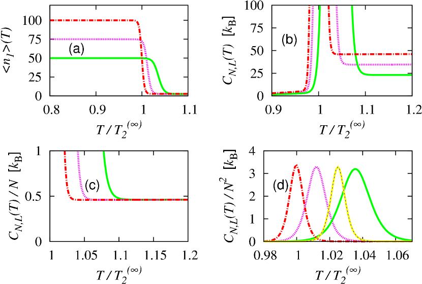
Figure 1: (Color online) Finite size investigations of the soliton–non-soliton transition for $N=50$ (green/gray solid line), $N=100$ (red/black dash-dotted line) and $N=75$ (magenta/gray dashed line) with $B=B_{0}$. (a) Size of the largest soliton (15) as a function of temperature. (b) For $N\approx 100$, the specific heat (14) as a function of temperature scales as $0.5k_{\rm B}$ at low temperatures indicating one bright soliton. (c) At high temperatures, it scales as $\lessapprox 0.5Nk_{\rm B}$, demonstrating a free gas of $N$ atoms. (d) The specific heat near the transition temperature scales as $N^{2}k_{\rm B}$. Excluding all states with more than one soliton (yellow/light gray line, $N=100$) clearly indicates the presence of several solitons near the transition temperature; the area of coexistence gets smaller for increasing $N$.

To demonstrate that we indeed have a phase transition let us start by focusing on cases where we have $N-n$ particles in one soliton and $n$ free particles; $n=\mathcal{O}(N)$ and $N\ggg 1$. Using Eq. (17) to express the partition function for $n$ free particles corresponds to a system with fewer atoms ($n$) but the same $g_{\rm 1D}$ thus rescaling $E_{\rm gap}$ and therefore also $T_{1,2}^{(\infty)}$ by a factor of $\frac{n^{2}}{N^{2}}$; the bounds in Eq. (16) now become for not too low temperatures

$$Z_{n,1,\rm kin}\left(\frac{1}{k_{\rm B}T_{2}^{(\infty)}}\right)\left(\frac{T}{T_{2}^{(\infty)}\frac{n^{2}}{N^{2}}}\right)^{\frac{n}{2}}\exp\left(\frac{(n+1)E_{\rm gap}}{3k_{\rm B}T_{2}^{(\infty)}}\right)\leq Z$$

$$\leq Z_{n,1,\rm kin}\left(\frac{1}{k_{\rm B}T_{1}^{(\infty)}\frac{n^{2}}{N^{2}}}\right)\left(\frac{T}{T_{1}^{(\infty)}\frac{n^{2}}{N^{2}}}\right)^{\frac{n}{2}}\exp\left(\frac{(n+1)E_{\rm gap}}{3k_{\rm B}T_{1}^{(\infty)}}\right),$$ (20)

with $Z=Z_{1,n,\rm kin}(\beta)$ and $T_{2}^{(\infty)}>T_{1}^{(\infty)}$. Multiplying this equation with $\exp[-\beta E_{0}(N-n)]$ to obtain the full partition function with $N-n$ particles in one soliton and $n$ free particles and dividing by $\exp[-\beta E_{0}(N)]$ yields that for $n\approx N$ the $n$-dependence (and in particular the question if they grow or shrink) is dominated by the $\left({T}/{T_{1,2}^{(\infty)}}\right)^{n/2}$-terms. Including factors of the order of (3) to include the contribution of all other configurations with $N-n$ particles in one soliton (or directly including terms with more than one small soliton) does not change the convergence behavior. Summing over $n\approx N$ such that the sum includes a finite fraction of $N$, say, all $n\geq 0.99N$, we thus have

$$0<\lim_{N\to\infty}\frac{\langle n_{1}\rangle}{N}\leq 1,\quad T<0.99^{2}T_{1}^{(\infty)}.$$ (21)

Extending the above reasoning based on Eq. (20) to high temperatures ($T>T_{2}^{(\infty)}$) shows that in the sum (15):

$$\lim_{N\to\infty}\frac{\langle n_{1}\rangle}{N}=0,\quad T>T_{2}^{(\infty)}.$$ (22)

Thus, using the canonical ensemble Pathria and Beale (2011) we have shown the existence of a phase transition in the thermodynamic limit (4) [cf. Fig. 2].

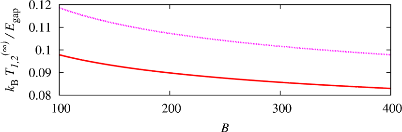
Figure 2: (Color online) Characteristic temperatures for the soliton–non-soliton transition in the thermodynamic limit (4) as a function of $B$ [Eq. (6) which depends on the ratio of the system size and the size of a two-particle soliton.]. Upper, magenta/gray dotted curve: above this temperature, the relative number of atoms in the largest soliton vanishes [Eq. (22)]. For temperatures below the red/black solid curve, a macroscopically occupied bright soliton exists [Eq. (21)]. The transition region is small compared to the difference of the two curves (cf. Fig. 1).

The $N$-dependence of the specific heat shows that both in the high-temperature phase [Fig. 1 (b),(c)] and in the low-temperature phase [Fig. 1 (b)] predictions of the canonical and the microcanonical ensemble Pathria and Beale (2011) agree Pathria and Beale (2011). As the mean energy is a monotonously increasing function of temperature [Eq. (14)] and as furthermore, the choice of the thermodynamic limit (4) leads to a mean energy $\propto N$ and an $N$-independent temperature scale, the $\propto N^{2}$ behavior displayed by the specific heat in Fig. 1 (d) can only occur in a small ($\propto 1/N$) temperature range in which both ensembles no longer are equivalent.

To conclude, we find the existence of a finite-temperature many-particle phase transition in a one-dimensional quantum many-particle model, the homogeneous Lieb-Liniger gas with attractive interactions [Eqs. (21) and (22); Fig. 2]. The low temperature phase consists of a macroscopic number of atoms being one large quantum matter-wave bright soliton with delocalized center-of-mass wave function (which does not display long-range order thus not violating the Mermin-Wagner theorem Mermin and Wagner (1966); Hohenberg (1967); the Landau criterion Lifshitz and Pitaevskii (2002) which argues against the co-existence of two distinct phases is also not violated); the high temperature phase is a free gas. As a harmonic trap would facilitate soliton formation Billam et al. (2012), we conjecture that the existence of a finite-temperature phase transition remains true for weak harmonic traps. In experiments, even the integrable Lieb-Liniger gas can thermalize as the wave guides are quasi-one-dimensional (cf. Mazets and Schmiedmayer (2010); Cockburn et al. (2011)).

Via exact canonical recurrence relations we also numerically investigate the experimentally relevant case of some 100 atoms (cf. Medley et al. (2014); Weiss and Castin (2009); Streltsov et al. (2009)) with the (experimentally realizable Schmidutz et al. (2014)) box potential. The spike-like specific heat provides further insight: the specific heat ($\propto N^{2}$) is the derivative (14) of an energy scaling not faster than $\propto N$ (4). At low temperatures all atoms form one soliton; the size of the soliton thus is an ideal experimental signature (cf. Khaykovich et al. (2002); Strecker et al. (2002); Cornish et al. (2006); Marchant et al. (2013); Medley et al. (2014); McDonald et al. (2014); Nguyen et al. (2014); Marchant et al. (2016); Everitt et al. (2015); Lepoutre et al. (2016)).