Evidence for magnetar formation in broad-lined type Ic supernovae 1998bw and 2002ap

Abstract

Broad-lined type Ic supernovae (SNe Ic-BL) are peculiar stellar explosions that distinguish themselves from ordinary SNe. Some SNe Ic-BL are associated with long-duration ($\gtrsim 2\mathord{\thinspace\rm s}$) gamma-ray bursts (GRBs). Black holes and magnetars are two types of compact objects that are hypothesized to be central engines of GRBs. In spite of decades of investigations, no direct evidence for the formation of black holes or magnetars has been found for GRBs so far. Here we report the finding that the early peak ($t\lesssim 50\mathord{\thinspace\rm days}$) and late-time ($t\gtrsim 300\mathord{\thinspace\rm days}$) slow decay displayed in the light curves of both SNe 1998bw (associated with GRB 980425) and 2002ap (not GRB-associated) can be attributed to magnetar spin-down with initial rotation period $P_{0}\sim 20\mathord{\thinspace\rm ms}$, while the intermediate-time ($50\lesssim t\lesssim 300\mathord{\thinspace\rm days}$) exponential decline is caused by radioactive decay of ⁵⁶Ni. The connection between the early peak and late-time slow decline in the light curves is unexpected in alternative models. We thus suggest that GRB 980425 and SN 2002ap were powered by magnetars.

1. Introduction

Broad-lined type Ic supernovae (SNe Ic-BL) are a subclass of core-collapse type Ic SNe (CCSNe) having broad absorption troughs in their optical spectra. Since their discovery, SNe Ic-BL stand out as a subclass that is peculiar compared with other ordinary CCSNe. One of their peculiarities is that their astonishing kinetic energy ($\sim 10^{52}\mathord{\thinspace\rm erg}$) is unexpected in the well-studied SN explosion mechanisms (Bethe, 1990; Janka et al., 2016).

Another peculiarity of SNe Ic-BL is the failure of one-dimensional ⁵⁶Ni model – which is assumed to work well for most of ordinary SNe Ibc – in reproducing their light curves. What is intricate in reproducing the light curves of SNe Ic-BL is that the simple analytical models have difficulty in modeling both the peak part and the later part. Most of the time different ⁵⁶Ni masses are derived, or multiple-zones need to be invoked (Maeda et al., 2003; Wheeler et al., 2015). In light of this difficulty, it was found that the light curve of SNe Ic-BL can be reasonably reproduced by proposing that the ejecta consist of two components, i.e. one fast-moving outer component which is responsible for the early peak and the inner slow compact component which produces the late-time exponential decline (Maeda et al., 2003). Such a two-component ⁵⁶Ni model is partially supported because of the asphericity suggested by polarization measurements (Patat et al., 2001) and peculiar nebular line profiles (Mazzali et al., 2001, 2005; Maeda et al., 2002, 2008) of some SNe Ic-BL. Hydrodynamic models of jetlike explosions (Nagataki et al., 1997; Khokhlov et al., 1999; MacFadyen & Woosley, 1999; Maeda et al., 2002) suggest a prolate spheroid. In such a scenario, a fast-moving component is produced along the jet, while the compact component is moving slowly along the perpendicular direction. Because of the energies of these two components are different, their synthesized ⁵⁶Ni masses are usually different.

SNe Ic-BL are also of great astrophysical importance because they are the only SNe in association with long-duration gamma-ray bursts (GRBs; Galama et al., 1998; Bloom et al., 1999; Hjorth et al., 2003; Stanek et al., 2003; Campana et al., 2006; Mazzali et al., 2006; Woosley & Bloom, 2006; Cano et al., 2016). Despite persistent investigation, there is still no direct evidence for the two types of hypothesized central engine of GRBs, i.e. black holes (Popham et al., 1999; Narayan et al., 2001; Kohri & Mineshige, 2002; Liu et al., 2007, 2016b; Song et al., 2016) and/or magnetars (Usov, 1992; Dai & Lu, 1998a, b; Zhang & Dai, 2008, 2009, 2010; Mösta et al., 2015). GRBs are usually collimated relativistic phenomena, while SNe Ic-BL are mostly subrelativistic and nearly isotropic. The remnants of all CCSNe are presumably black holes or neutron stars. The light curve of an SN powered by a black hole (Dexter & Kasen, 2013; Gao et al., 2016) is different from that powered by a magnetar. Therefore SNe Ic-BL could shed light on the still elusive central engine of GRBs.

There is indirect evidence that SNe Ic-BL are powered by millisecond magnetars because their kinetic energy has an upper limit that is close to the rotational energy of a neutron star spinning at nearly broken-up frequency (Mazzali et al., 2014). Furthermore, the progenitor mass of SN 2006aj associated with GRB 060218 (Mazzali et al., 2006) and the light curve of SN 2011kl associated with GRB 111209A (Greiner et al., 2015) are consistent with magnetar formation. Nonetheless, the modeling uncertainty of stellar evolution for SN 2006aj (Mazzali et al., 2006) and the short-duration data coverage ($t\lesssim 60\mathord{\thinspace\rm days}$) and moderate data accuracy for SN 2011kl (Greiner et al., 2015) make such evidence inconclusive.

In developing a magnetar model for SNe Ic-BL, it is found for SNe 1997ef and 2007ru that the early rapid rise and decline ($t\lesssim 50\mathord{\thinspace\rm days}$) in the light curves stems from the contribution of a rapidly spinning magnetar, while the later exponential decline ($50\lesssim t\lesssim 200\mathord{\thinspace\rm days}$) can be attributed to the ⁵⁶Co radioactive decay (Wang et al., 2016b). This model reduces the total ⁵⁶Ni mass needed to power the light curve and therefore solves the long-lasting problem for the magnetar model that the shock caused by the spin-down of a magnetar cannot synthesize the needed ⁵⁶Ni (Nishimura et al., 2015; Suwa & Tominaga, 2015). In addition, this model naturally provides the huge kinetic energy of SNe Ic-BL by converting most of the magnetar’s rotational energy into kinetic energy of the ejecta. The successful demonstration of the magnetar model in reproducing the light curves of SNe Ic-BL is a supportive evidence for magnetar formation in SNe Ic-BL. However, we have to bear in mind that the magnetar model is only one possible choice for SNe Ic-BL because the two-component model is also able to reproduce reasonably well the light curves of most SNe Ic-BL (Maeda et al., 2003).

The motivation for this work is, on the one hand, to assess the ability of the magnetar model in reproducing the very late-phase ($t\gtrsim 300\mathord{\thinspace\rm days}$) light curves of SNe Ic-BL when the luminosity decline rate shows evidence for deviation from the exponential decline (during the phase $50\lesssim t\lesssim 200\mathord{\thinspace\rm days}$) and on the other hand to compare it with the two-component model.

The reason for observational data for $t\gtrsim 300\mathord{\thinspace\rm days}$ is as follows. If one focuses on the data within one year after explosion, the $t^{-2}$ tail in the magnetar model easily parallels that expected from ⁵⁶Co decay and one cannot unambiguously tell if it is the magnetar or ⁵⁶Co that is powering the light curve (Woosley, 2010; Inserra et al., 2013). Only at very late phases can one distinguish between magnetar model and ⁵⁶Co decay model.

To accurately determine the parameter values, a Markov chain Monte Carlo program is developed. We search the literature and find that SNe 1998bw and 2002ap have an observational coverage well beyond $500\mathord{\thinspace\rm days}$ and are therefore quite suitable for our investigation. To our surprise, in Section 2 it is found that in the magnetar model, the magnetar not only contributes to the early peak of the light curve of the broad-lined SNe 1998bw and 2002ap, but it can also manifest itself as a significant excess over the exponential decay in late-time light curves when the ⁵⁶Co contribution became small compared to the magnetar spin-down luminosity. The results are discussed in Section 3 and it is argued that SNe 1998bw and 2002ap provide hitherto strong evidence for magnetar formation in SNe Ic-BL. A short summary is given in Section 4.

2. Data preparation and modeling

Being one of the nearest SNe in the last decades, SN 2002ap triggered an observational campaign since its discovery on 2002 January 29 (Gal-Yam et al., 2002; Mazzali et al., 2002; Foley et al., 2003; Yoshii et al., 2003; Tomita et al., 2006). Thanks to its proximity, only $9.4\mathord{\thinspace\rm Mpc}$ in distance, high quality observational data were acquired until $580\mathord{\thinspace\rm days}$ after explosion, which is prerequisite for the identification of late excess over the exponential ⁵⁶Co decay.

SN 1998bw (Galama et al., 1998; McKenzie & Schaefer, 1999; Sollerman et al., 2000; Patat et al., 2001; Clocchiatti et al., 2011), on the other hand, is the nearest SN associated with a GRB (Cano et al., 2016). Although at a distance greater than SN 2002ap, its brighter luminosity qualifies SN 1998bw as an ideal observational target and its light curve was measured to $\sim 1000\mathord{\thinspace\rm days}$ post explosion (Sollerman et al., 2002).

To accurately model the light curve of SNe 1998bw and 2002ap, we develop a Markov chain Monte Carlo approach based on the recently updated analytic magnetar model (Wang et al., 2016c). In this model, photospheric recession is considered so that the photospheric velocity evolution is traced. The acceleration of the SN ejecta by the magnetar energy injection is taken into account. That is, in this model the kinetic energy of the SNe Ic-BL is believed to originate mainly from the magnetar spin-down. Nevertheless, this does not preclude the possibility of a non-zero initial explosion energy. This model also incorporates the high energy photon leakage (Wang et al. 2015b, see also Chen et al. 2015) based on the fact that the energy injection emanated from the magnetar could be dominated by high energy photons (Bühler & Blandford, 2014; Wang et al., 2016a).

In summary, aside from the usual parameters, e.g. the ejecta mass $M_{\mathrm{ej}}$, the ⁵⁶Ni mass $M_{\mathrm{Ni}}$, the opacity in optical band $\kappa$, we also need the opacity $\kappa_{\gamma,\mathrm{Ni}}$ to ⁵⁶Ni (including ⁵⁶Co) decay photons, the opacity $\kappa_{\gamma,\mathrm{mag}}$ to magnetar photons and the magnetar parameters, i.e. the dipole magnetic field $B_{p}$ and initial rotation period $P_{0}$.

The optical opacity $\kappa$ is strongly degenerated with the ejecta mass $M_{\mathrm{ej}}$ and cannot be accurately determined in this model. Fortunately, $\kappa$ is a parameter that characterizes the microphysics of the ejecta and therefore can be calculated in first principles based on our knowledge about the ejecta composition. It is believed that the progenitor of an SN Ic (broad-lined or not) is a massive single star or a low-mass star in a binary (Smartt, 2009). The ejecta of such a star explosion are mainly composed of ¹⁶O, ²⁰Ne and ²⁴Mg (Iwamoto et al., 2000; Nakamura et al., 2001a; Maeda et al., 2002). In the literature a range of values, from $0.06\mathord{\thinspace\rm cm}^{2}\mathord{\thinspace\rm g}^{-1}$ to $0.2\mathord{\thinspace\rm cm}^{2}\mathord{\thinspace\rm g}^{-1}$, is used for such a composition (e.g., Wang et al., 2015c; Dai et al., 2016, and references therein). Here we adopt the constant value $\kappa=0.1\mathord{\thinspace\rm cm}^{2}\mathord{\thinspace\rm g}^{-1}$. We note that the optical opacity is also a function of the ionization state of the ejecta. A magnetar sitting in the center of the explosion provides a source of ionizing radiation (Metzger et al., 2014; Wang et al., 2016a) and therefore the ejecta could be ionized even when they are cooled to a low temperature. This means that the late-time ionization level of the ejecta powered by a magnetar is usually higher than that powered by radioactive decay. A high level of ionization inclines to keep the optical opacity constant over a long time. We therefore suggest that a constant optical opacity is appropriate in the magnetar model.

The opacity to ⁵⁶Ni decay photons $\kappa_{\gamma,\mathrm{Ni}}$ usually takes the fiducial value $\kappa_{\gamma,\mathrm{Ni}}=0.025-0.027\mathord{\thinspace\rm cm}^{2}\mathord{\thinspace\rm g}^{-1}$ (Colgate et al., 1980; Swartz et al., 1995). In the actual applications it is found from case to case that this value cannot fit the light curve of some SNe (e.g., Filippenko & Sargent, 1986; Tsvetkov, 1986; Schlegel & Kirshner, 1989; Swartz & Wheeler, 1991; Wang et al., 2016b). This discrepancy may be caused by some macrophysical ignorance, e.g. a peculiar density distribution of the ejecta. In this work we leave $\kappa_{\gamma,\mathrm{Ni}}$ as a free parameter and appreciate its deviation from the fiducial value as macrophysical uncertainties.

Another more uncertain parameter is the opacity to magnetar photons $\kappa_{\gamma,\mathrm{mag}}$. Depending on the energy spectra of the spinning magnetar, $\kappa_{\gamma,\mathrm{mag}}$ may vary from $10^{-2}\mathord{\thinspace\rm cm}^{2}\mathord{\thinspace\rm g}^{-1}$ to $10^{6}\mathord{\thinspace\rm cm}^{2}\mathord{\thinspace\rm g}^{-1}$ (Kotera et al., 2013). Based on this fact, we set $\kappa_{\gamma,\mathrm{mag}}$ as a free parameter.

In the previous magnetar modeling to demonstrate that the early light curve of SNe Ic-BL is due to the contribution of a magnetar, we assume that the kinetic energy of SNe Ic-BL comes exclusively from the magnetar spin-down (Wang et al., 2016b). This is approximately true for the SNe studied by Wang et al. (2016b) because the rapid rise in the light curve of SNe 1997ef and 2007ru precludes a significant initial explosion energy. In a more general case, however, any SN explosion should have an initial explosion energy. Consequently, we parameterize the initial explosion energy by including an initial expansion velocity $v_{\mathrm{sc}0}$ in our model.

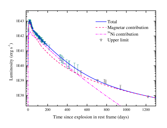
Figure 1.— Best-fit light curve (solid line) of SN 1998bw. The dashed line (the magnetar contribution) is the light curve with $M_{\mathrm{Ni}}=0$ while other parameters take the same values as the solid line. The dot-dashed line is the difference between these two light curves, i.e., the ⁵⁶Ni contribution. The data points ($t<506\mathord{\thinspace\rm days}$) are taken from Patat et al. (2001). In this figure we do not try to fit the dark star data points and the two upper limits. They are taken from Sollerman et al. (2002) after shifted upward by $0.6\mathord{\thinspace\rm dex}$ and plotted here just for eye guidance. See the text for more explanation.

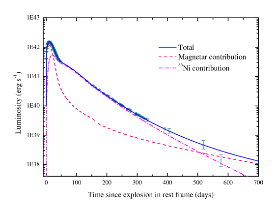
Figure 2.— Same as Figure 1, but for SN 2002ap.

Table 1Best-fit parameters for SNe 1998bw and 2002ap. The uncertainties are $1\sigma$ errors.

SN	$M_{\mathrm{ej}}$	$M_{\mathrm{Ni}}$	$B_{p}$	$P_{0}$	$v_{\mathrm{sc}0}$	$\kappa_{\gamma,\mathrm{Ni}}$	$\kappa_{\gamma,\mathrm{mag}}$	$T_{\mathrm{start}}$	$E_{K}$
	$\left(M_{\odot}\right)$	$\left(M_{\odot}\right)$	$\left(10^{15}\mathord{\thinspace\rm G}\right)$	$\left(\mathord{\thinspace\rm ms}\right)$	$\left(\mathord{\thinspace\rm km}\mathord{\thinspace\rm s}^{-1}\right)$	$\left(\mathord{\thinspace\rm cm}^{2}\mathord{\thinspace\rm g}^{-1}\right)$	$\left(\mathord{\thinspace\rm cm}^{2}\mathord{\thinspace\rm g}^{-1}\right)$	$\left(\mathord{\thinspace\rm days}\right)$	$\left(10^{51}\mathord{\thinspace\rm erg}\right)$
1998bw	$2.6_{-0.4}^{+0.5}$	$0.10_{-0.02}^{+0.03}$	$1.66_{-0.14}^{+0.21}$	$20.8\pm 0.4$	$11040_{-1591}^{+1501}$	$0.31_{-0.11}^{+0.14}$	$0.29_{-0.17}^{+0.19}$	$-0.009_{-0.36}^{+0.32}$	$1.86$
2002ap	$2.0_{-0.36}^{+0.14}$	$0.029\pm 0.0004$	$13.7\pm 0.3$	$22.2_{-1.2}^{+1.3}$	$8134_{-1878}^{+344}$	$0.08_{-0.017}^{+0.003}$	$5.3_{-2.3}^{+2.0}$	$1.5_{-0.07}^{+0.06}$	$0.79$

Note. In these fits, we fix $\kappa=0.1\mathord{\thinspace\rm cm}^{2}\mathord{\thinspace\rm g}^{-1}$. The parameters on the left side of the vertical line are fitting values, while the one on the right side is derived from the fitting values.

a. Ejecta mass.

b. ⁵⁶Ni mass.

c. Magnetic dipole field strength of the magnetar.

d. Initial rotation period of the magnetar.

e. Initial expansion velocity of the ejecta.

f. Opacity to ⁵⁶Ni decay photons.

g. Opacity to magnetar spin-down photons.

h. Explosion time relative to the observational data.

i. Initial explosion energy.

Because we usually do not know the explosion time of the SN, we include a parameter, the explosion time $T_{\mathrm{start}}$, in the Monte Carlo program. For SN 1998bw, the explosion time is known and in this case we can actually evaluate the validity of the fitting procedure by comparing the determined $T_{\mathrm{start}}$ with the actual explosion time.

The luminosity data points for SN 2002ap are taken from Tomita et al. (2006). The luminosity observational errors are all taken from Figure 4 of Tomita et al. (2006), i.e., $\pm 0.03\mathord{\thinspace\rm mag}$ except for the last five points. The photospheric velocity data are taken from Gal-Yam et al. (2002) and Mazzali et al. (2002). The uncertainties in the measurement of photospheric velocity is usually large (cf. Figure 8 of Valenti et al., 2008). In view of this fact, we adopt the measurement error in photospheric velocity as half of the measured value.

The data points for SN 1998bw up to $506\mathord{\thinspace\rm days}$ after explosion, including the UVOIR bolometric luminosity data and photospheric velocity data, are taken from Patat et al. (2001). Sollerman et al. (2002) obtained OIR luminosity up to $\sim 1000\mathord{\thinspace\rm days}$ post explosion (their Figure 4). Because of the missing of $UV$ band data in the light curve of Figure 4 in Sollerman et al. (2002), we do not try to fit the data from Sollerman et al. (2002). Nevertheless, we try to compare the data from Patat et al. (2001) and Sollerman et al. (2002) and find that the data at $t\sim 500\mathord{\thinspace\rm days}$ can be bring consistent with each other if the data given by Sollerman et al. (2002) are shifted $0.6\mathord{\thinspace\rm dex}$ upward. This treatment of the data from Sollerman et al. (2002) is not accurate enough because the multiplicative factors at different phases should be different. In view of this fact we do not try to fit these shifted data and upper limits in Figure 1 and plot them here just for eye guidance. The difference between the data from Patat et al. (2001) and Sollerman et al. (2002) at similar times can be attributed to several factors. First of all, the contribution from $UV$ band is substantial and cannot be neglected even at these advanced stages. Second, it was found that the measured decay rates in $R$ and $I$ bands during the stage $300-500\mathord{\thinspace\rm days}$ are different between Patat et al. (2001) and Sollerman et al. (2002). Sollerman et al. (2002) attributed this difference to different background subtraction strategy. Third, Patat et al. (2001) adopted a larger distance to SN 1998bw ($37.8\mathord{\thinspace\rm Mpc}$) than Sollerman et al. (2002) ($35\mathord{\thinspace\rm Mpc}$). Finally, because of the missing of measurements in $IR$ band, these two groups of authors assumed different contribution from $IR$ band to the bolometric luminosities.

Our modeling result is presented in Figures 1 and 2 with the best-fit parameters listed in Table 1. In Figure 1 we plot the data from Sollerman et al. (2002) as dark stars and two upper limits, after shifted upward by $0.6\mathord{\thinspace\rm dex}$.

Figures 1 and 2 indicate that the early peaks are caused by the magnetar injection, as already found by Wang et al. (2016b). During the period from day 50 to day $\sim 300$ after explosion, the SN light curve follows closely the ⁵⁶Co exponential decay. After $\sim 300\mathord{\thinspace\rm days}$ the light curve systematically deviates from this exponential decay. What is surprising to us is that the late-time deviation from the exponential decay can be curiously accounted for by the magnetar contribution. This connection between early peak and late-time slow decay of the light curve is unexpected in the two-component model (Maeda et al., 2003).

In developing the magnetar model, to obtain an analytical result, the temperature distribution within the ejecta is separated in space and time coordinates (see Appendix of Wang et al., 2016c), $T\left(r,t\right)^{4}\propto\psi\left(x\right)\phi\left(t\right)$, where $\psi\left(x\right)$ is a dimensionless function of mass coordinate $x$ that characterizes the radiation energy per unit volume. The heating rate is similarly separated $\epsilon\left(r,t\right)=\xi\left(x\right)f\left(t\right)$, where $\xi\left(x\right)$ is another dimensionless function that characterizes the volume emission after multiplied by the dimensionless density $\eta\left(x\right)$. We assume that the volume emission of the heating sources, including magnetar injection and ⁵⁶Ni heating, is proportional to the radiation energy per unit volume, i.e. $\xi\left(x\right)\eta\left(x\right)\propto\psi\left(x\right)$ as suggested originally by Arnett (1982) in developing an analytical model for ordinary (⁵⁶Ni only) type I SNe (assuming the quantity in Equation [13] of Arnett 1982 a constant). This assumption is not strictly true, but it is a good approximation which captures the main feature of thermalization of the magnetar radiation and ⁵⁶Ni decay photons.

When isolating the ⁵⁶Ni contribution to the light curve, we actually perform a subtraction between two light curves, the full light curve (including magnetar and ⁵⁶Ni) and the magnetar-only light curve. We do not calculate the ⁵⁶Ni light curve by turning off the magnetar contribution because the magnetar could provide a substantial contribution to the ejecta kinetic energy and the evolution of the ejecta expansion velocity impacts the resulting light curve. Due to this fact, one is not encouraged to directly compare the ⁵⁶Ni contribution to a real ⁵⁶Ni light curve.

There seems to be a little bump in the magnetar component around 150 days in Figure 2. This bump occurs at the time when the SN is transitioning to the full nebular phase. The rapid recession of the photosphere cannot be handled accurately by the finite time step in the numerical code. The real curve for the magnetar contribution should be very smooth and one should therefore ignore this numerical artifact.

3. Discussion

There were attempts to reproduce the light curve of SN 1998bw by a pure-magnetar model and pure-⁵⁶Ni model (Figure 19 of Inserra et al., 2013). The failure of these models calls for alternative models for SNe Ic-BL, manifesting the investigation of magnetar plus ⁵⁶Ni model presented in this work.

The idea of combining a magnetar and ⁵⁶Ni to reproduce the light curve of SN 1998bw was previously discussed by Woosley (2010). By considering the luminosity of SN 1998bw at $1000\mathord{\thinspace\rm days}$, Woosley (2010) estimated that the magnetar would be born with a field strength in excess of $8\times 10^{15}\mathord{\thinspace\rm G}$. It was estimated that a magnetar with such a strong field will loss all of its rotational energy to explosion and none left to the light curve. However, it is recently shown that such an estimate is only partially correct (Wang et al., 2016b). On the one hand, with a much strong magnetic field, the magnetar is indeed prone to losing its energy to explosion (Wang et al., 2016c). On the other hand, however, a minor fraction of the rotational energy will be thermalized, which is enough to power the light curve (Wang et al., 2016b).

In the magnetar (plus ⁵⁶Ni) model, the intermediate-time ($50\lesssim t\lesssim 300\mathord{\thinspace\rm days}$) exponential decay, sensitive to the ⁵⁶Ni mass $M_{\mathrm{Ni}}$, in the light curve is caused by ⁵⁶Co decay, while in the two-component model this exponential decay is assumed to be produced by the inner component. It is therefore desirable to compare the value $M_{\mathrm{Ni}}$ in the magnetar model to the ⁵⁶Ni mass of the inner component in the two-component model. Comparison of Table 1 with Table 2 of Maeda et al. (2003) shows good agreement between $M_{\mathrm{Ni}}$ in the magnetar model and the inner component ⁵⁶Ni mass $M\left({}^{56}\mathrm{Ni}\right)_{\mathrm{in}}$ in the two-component model. We note that unusually strong nebular lines of [Fe II] are seen in SN 1998bw, consistent with the production of more than the usual amount of Fe in the explosion (Mazzali et al., 2001). This is first of all in accord with the magnetar model because the inferred ⁵⁶Ni mass of SN 1998bw is indeed larger than the ⁵⁶Ni masses found in other SNe Ic-BL, e.g. SNe 1997ef, 2007ru, 2002ap, within the magnetar model. On the other hand, though, the synthetic SN spectra suffer from large modeling uncertainties and a ⁵⁶Ni mass of $0.1M_{\odot}$ is not inconsistent with observation. In the two-component model, the inferred total ⁵⁶Ni mass, $\sim 0.5M_{\odot}$, implies a progenitor core mass $\sim 3M_{\odot}$ (Nakamura et al., 2001a, b), which is in excess of the maximum mass of a neutron star, suggesting a collapsar (black hole) for GRB 980425. In the magnetar model, however, the total ⁵⁶Ni mass, $0.1M_{\odot}$, is consistent with the formation of a magnetar. This also serves as a self-consistent check for the magnetar model.

Except for the ⁵⁶Ni mass, other parameters could be significantly different between these two models. For SN 2002ap, the ejecta mass in the magnetar model is in reasonable agreement with the total ejecta mass given in the two-component model, while the ejecta mass of SN 1998bw in the magnetar model is significantly smaller than that given by Maeda et al. (2003). Table 1 shows that, in the magnetar model, $M_{\mathrm{ej}}\left(\mathrm{SN\quad 1998bw}\right)\approx M_{\mathrm{ej}}\left(\mathrm{SN\quad 2002ap}\right)$. This result seems hard to understand. However, when we compare the light curves of these two SNe (Tomita et al., 2006), it is immediately evident that both the early and late-time shape of the light curve of SN 2002ap is strikingly similar to that of SN 1998bw. In other words, SN 1998bw is just a brighter cousin to SN 2002ap. These two SNe have the same rise and decline rate around the peak time. The fact that SN 1998bw has a slightly heavier ejecta mass is only because, in the light curve modeling aspect, it expanded faster than SN 2002ap. Such a parameter difference for SN 1998bw between the two-component model and the magnetar model may imply a difference for its progenitor. The ejecta mass, $10M_{\odot}$, in the two-component model points to a massive single star, while $M_{\mathrm{ej}}=2.6M_{\odot}$ in the magnetar model favors a binary origin (Fremling et al., 2016), although a $\sim 4M_{\odot}$ Wolf-Rayet star (here a remnant magnetar with typical mass $1.4M_{\odot}$ is assumed) evolved from a single $35M_{\odot}$ main sequence star is also possible (Woosley & Heger, 2007; Woosley, 2010).

The initial kinetic energy in the magnetar model is $7.9\times 10^{50}\mathord{\thinspace\rm erg}$ and $1.86\times 10^{51}\mathord{\thinspace\rm erg}$ for SNe 2002ap and 1998bw, respectively. These values are significantly smaller than that given by the two-component model (Maeda et al., 2003) and in expectation from neutrino heating (Janka et al., 2016).

The magnetic dipole field strength $B_{p}=\left(13.7\pm 0.3\right)\times 10^{15}\mathord{\thinspace\rm G}$ for SN 2002ap is similar to the value determined for SN 1997ef, while the value $B_{p}=\left(1.66_{-0.14}^{+0.21}\right)\times 10^{15}\mathord{\thinspace\rm G}$ for SN 1998bw is significantly smaller. The weaker magnetic field for SN 1998bw is required because of its brighter luminosity (Wang et al., 2016b). Usually a magnetar can have dipole field in the range $10^{14}-10^{15}\mathord{\thinspace\rm G}$ (Mereghetti, 2008). However, it is suggested that a dipole field as strong as $\sim 10^{16}\mathord{\thinspace\rm G}$ is possible in theoretical aspects (Wang et al., 2016b).

In this fitting a value $\kappa_{\gamma,\mathrm{mag}}\gtrsim 2\mathord{\thinspace\rm cm}^{2}\mathord{\thinspace\rm g}^{-1}$ is favoured for SN 2002ap. But in practice it is found that $\kappa_{\gamma,\mathrm{mag}}=2\mathord{\thinspace\rm cm}^{2}\mathord{\thinspace\rm g}^{-1}$ and $\kappa_{\gamma,\mathrm{mag}}=6\mathord{\thinspace\rm cm}^{2}\mathord{\thinspace\rm g}^{-1}$ result in essentially the same light curve. This fact can also be appreciated by inspecting Figure 4. From Table 1 we see a large difference of $\kappa_{\gamma,\mathrm{mag}}$ between SNe 1998bw and 2002ap. Inspection of Figure 8 of Kotera et al. (2013) indicates that this could imply average magnetar photon energies $\sim 10-100\mathord{\thinspace\rm keV}$, in agreement with observation (Hester, 2008). Theoretically, magnetar radiation depends on several parameters, e.g., magnetic field, rotation period, angle between rotation axis and magnetic axis, and theorists are still struggling to unequivocally predict its spectrum energy distribution (Kennel & Coroniti, 1984a, b; Lyubarsky & Kirk, 2001; Wang & Dai, 2013; Kargaltsev et al., 2015; Murase et al., 2015; Wang et al., 2015a, 2016a; Liu et al., 2016a).

It can be seen that the two values of $\kappa_{\gamma,\mathrm{Ni}}$ are also different and larger than the fiducial value $\kappa_{\gamma,\mathrm{Ni}}\approx 0.03\mathord{\thinspace\rm cm}^{2}\mathord{\thinspace\rm g}^{-1}$. We think of this as macrophysical uncertainties, e.g., a clumpy density distribution. Radiation hydrodynamic calculations show that the magnetar-driven ejecta pile up at some radius (Kasen & Bildsten, 2010), rather than homogeneously distributed, as assumed in this work.

As stated above, the validity of the fitting program can also be appreciated by comparing the determined value of explosion time $T_{\mathrm{start}}$ with the actual explosion time. For SN 1998bw whose explosion time is known, the best-fit result gives $T_{\mathrm{start}}=-0.009_{-0.36}^{+0.32}\mathord{\thinspace\rm days}$, in excellent agreement with observations. Such a consistency also confirms the association of SN 1998bw with GRB 980425.

Inspection of Figures 1 and 2 shows that the Monte Carlo program sensitively captures the shape changes in the light curve. The decline rate of the light curve of SN 2002ap changes from $0.018\mathord{\thinspace\rm mag}\mathord{\thinspace\rm day}^{-1}$ between days 130 and 230 to $0.014\mathord{\thinspace\rm mag}\mathord{\thinspace\rm day}^{-1}$ between days 270 and 580 (Tomita et al., 2006). There is a similar change in the light curve of SN 1998bw between phase ranges 40-330 and 300-490 (see Table 4 of Patat et al., 2001). The flattening in the phase range 500-1200 of SN 1998bw (see Figure 1) is actually a “prediction” of the magnetar model because we do not fit these data.

A number of effects were discussed that may contribute to this flattening, including light echoes (Cappellaro et al., 2001; Andrews et al., 2015; Van Dyk et al., 2015), interaction with circumstellar medium (Chevalier, 1982; Chevalier & Fransson, 1994; Ginzburg & Balberg, 2012; Wang et al., 2016d), emission from surviving binary star companion (Kochanek, 2009; Pan et al., 2014), radioactive isotopes (Woosley et al., 1989; Sollerman et al., 2002; Seitenzahl et al., 2009), clumping (Maeda et al., 2003; Tomita et al., 2006), positron escape (Clocchiatti et al., 2008; Leloudas et al., 2009), freeze-out of the steady state approximation (Clayton et al., 1992; Fransson & Kozma, 1993), radiation transport for late SNe Ia (Fransson & Jerkstrand, 2015), contribution from an H II region or individual stars (Patat et al., 2001), aspherical geometry (Maeda et al., 2002, 2006), gamma-ray trapping (Clocchiatti & Wheeler, 1997; Nakamura et al., 2001a), magnetar field decay (Woosley, 2010), or contributions from collisions or a GRB afterglow (Bloom et al., 1999).

Among all of the above possibilities, Sollerman et al. (2002) considered a simple but plausible case of ⁵⁷Co and ⁴⁴Ti radioactive contributions to the flattening, although with a ratio of ⁵⁷Ni/⁵⁶Ni three times larger than the ratio observed in SN 1987A. Indeed, these radioactive flattening resembles a magnetar powering at $t\approx 1200\mathord{\thinspace\rm days}$ because of the progressive contributions from ⁵⁶Co, ⁵⁷Co and ⁴⁴Ti at later phases (Arnett et al., 1989).

In comparison to the above models, it was recently shown that in the magnetar model $B_{p}$ and $P_{0}$ can be accurately determined by the early peak for those SNe whose peak is caused by a spinning-down magnetar (Wang et al., 2016b). The advantage of the magnetar model over the two-component model is the fact that the magnetar parameters, $B_{p}$ and $P_{0}$, determined by the early peak can naturally account for the late-time slow decline in the light curves of SNe 1998bw and 2002ap. The magnetar initial rotation periods $P_{0}\sim 20\mathord{\thinspace\rm ms}$ for SNe 1998bw and 2002ap are longer than that of SN 1997ef (Wang et al., 2016b). This longer $P_{0}$ of the magnetar is required for a relatively slow rise (compared to SNe 1997ef and 2007ru) of the peak in the light curve. This $P_{0}$ is also essential for its contribution to the late-time observable excess relative to the ⁵⁶Co exponential decay. In other words, the magnetar model predicts that the rise rate in early-time light curve should be relatively slow if the SN has a long lasting flattening. This intrinsic connection between the early peak and late-time flattening is not expected in alternative models and therefore provides a strong evidence in favor of the magnetar model.

It may be argued that the magnetar model presented here can give a better account for these two SNe because there are more free parameters in this model. This is not simply true at its first glance. There are 8 free parameters in the magnetar model (see Table 1). In the two-component model, the free parameters include $v_{\mathrm{in}}$, $M_{\mathrm{in}}$, $M\left({}^{56}\mathrm{Ni}\right)_{\mathrm{in}}$, $v_{\mathrm{out}}$, $M_{\mathrm{out}}$, $M\left({}^{56}\mathrm{Ni}\right)_{\mathrm{out}}$, $T_{\mathrm{start}}$. To account for the late flattening, provided that it is attributed to ⁵⁷Co and ⁴⁴Ti, another two parameters, $M\left({}^{57}\mathrm{Co}\right)$ and $M\left({}^{57}\mathrm{Ti}\right)$, are needed. It is 9 parameters in total.

SNe Ic-BL show some evidence of asphericity, especially those associated with GRBs. In this case the early peak of the light curve may contain a fraction of contribution by the fast-moving material in the ejecta. The peak luminosity of an SN is sensitive to the dipole magnetic field $B_{p}$. The contribution of the asphericity would increase $B_{p}$ so that the magnetar deposits less of its rotational energy into the light curve. Nevertheless the observed polarization $0.5\%$ of SN 1998bw at optical wavelengths can be explained by an axial ratio less than $2:1$ (Höflich, 1995; Höflich et al., 1999). Such asphericity is actually comparable to the well-observed nearby SN 1987A (Larsson et al., 2016). This indicates that the departure from spherical symmetry of the optically emitting material is only moderate.

4. Conclusions

The identification of the central engine of GRBs has long been a challenge in high-energy astrophysics. Instead of investigating the prompt emission and afterglows of GRBs, here we try to figure out what can be inferred by studying the light curves of SNe Ic-BL. Stimulated by frequent hinds of magnetar formation in GRBs and SNe Ic-BL, we present a magnetar (plus ⁵⁶Ni) model for SNe Ic-BL and find evidence that SNe Ic-BL 1998bw and 2002ap were powered by magnetars.

In more than one decade the picture of ⁵⁶Ni heating to power the light curves of SNe Ic-BL was developed, with two-component model the most outstanding. Here we present evidence that magnetars could be a more natural alternative. The two-component model does not account for the origin of the huge kinetic energy of SNe Ic-BL. The magnetar model, on the contrary, provides a complete solution for energetics, ${}^{56}\mathrm{Ni}$ synthesis, and light curves. It is still to see if the spectra of SNe Ic-BL are consistent with the magnetar model. We note that the nebular spectra of SN 1998bw at days until about 337 post explosion have a wide bump in the region between 4000 and 5500$\mathord{\thinspace\rm\text{\AA}}$ (Patat et al., 2001). Such a feature is consistent with magnetar model.

To bring the magnetar model for SNe Ic-BL onto a more solid ground, additional information is necessary. For example, the continuous injection of magnetar energy at late time should affect the emission line width evolution (Chevalier & Fransson, 1992). Future high accuracy multi-messenger observations can also help identify the newborn magnetars in SNe Ic-BL (Kashiyama et al., 2016).

We note in passing that another SN Ic-BL that was observed to late stage $t>300\mathord{\thinspace\rm days}$ is SN 2003jd (Valenti et al., 2008). However, because of the sparse coverage of the observational data, we do not try to fit and analyze it in this work. It is evident that SN 2003jd also displays a change in decline rate between stages 50-100 and 300-400 (Valenti et al., 2008), indicative of magnetar formation. This may indicate that magnetar is a common remnant in SNe Ic-BL.

Appendix A Parameter uncertainties

To help understand the parameter uncertainties and their degeneracy, we plot the parameter corner graphs in Figures 3 and 4. Figure 3 shows that $\kappa_{\gamma,\mathrm{mag}}\lesssim 0.5\mathord{\thinspace\rm cm}^{2}\mathord{\thinspace\rm g}^{-1}$ is favored but it cannot be constrained tightly. This is because the observational errors during the period 300-500 days are relatively large, as can be seen from Figure 1. Figure 4 indicates some degeneracy between $T_{\mathrm{start}}$ and $P_{0}$, $B_{p}$. This is easily understood because $P_{0}$ and $B_{p}$ determine the rising rate of the light curve. This figure also shows that $\kappa_{\gamma,\mathrm{mag}}$ should not be less than $\sim 2\mathord{\thinspace\rm cm}^{2}\mathord{\thinspace\rm g}^{-1}$.

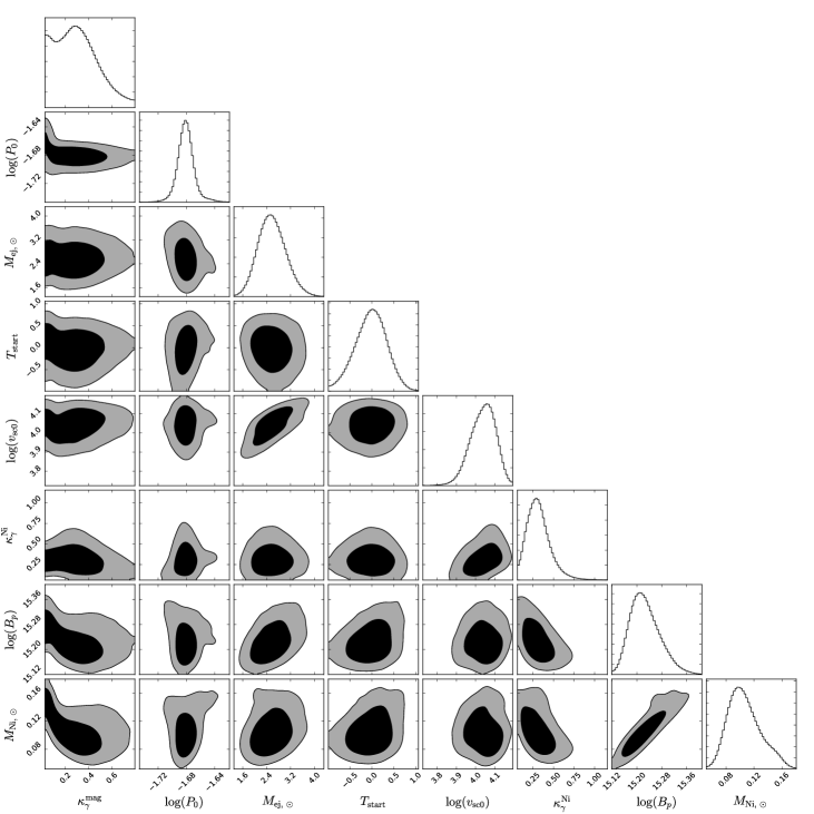
Figure 3.— Parameter corner in the modeling of SN 1998bw. The contours are $1\sigma$ and $2\sigma$ uncertainties, respectively.

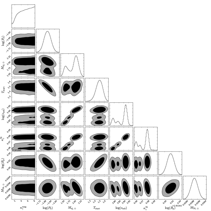
Figure 4.— Parameter corner in the modeling of SN 2002ap.

References

- Andrews et al. (2015) Andrews, J. E., Smith, N., & Mauerhan, J. C. 2015, MNRAS, 451, 1413
- Arnett (1982) Arnett, W. D. 1982, ApJ, 253, 785
- Arnett et al. (1989) Arnett, W. D., Bahcall, J. N., Kirshner, R. P., & Woosley, S. E. 1989, ARA&A, 27, 629
- Berger et al. (2002) Berger, E., Kulkarni, S. R., & Chevalier, R. A. 2002, ApJL, 577, L5
- Bethe (1990) Bethe, H. A. 1990, RvMP, 62, 801
- Bloom et al. (1999) Bloom, J. S., Kulkarni, S. R., Djorgovski, S. G., et al. 1999, Natur, 401, 453
- Brown et al. (2016) Brown, P. J., Breeveld, A., Roming, P. W. A., & Siegel, M. 2016, AJ, 152, 102
- Bühler & Blandford (2014) Bühler, R., & Blandford, R. 2014, RPPh, 77, 066901
- Campana et al. (2006) Campana, S., Mangano, V., Blustin, A. J., et al. 2006, Natur, 442, 1008
- Cano (2013) Cano, Z. 2013, MNRAS, 434, 1098
- Cano et al. (2016) Cano, Z., Wang, S. Q., Dai, Z. G., & Wu, X. F. 2016, arXiv:1604.03549
- Cappellaro et al. (2001) Cappellaro, E., Patat, F., Mazzali, P. A., et al. 2001, ApJL, 549, L215
- Chakraborti et al. (2015) Chakraborti, S., Soderberg, A., Chomiuk, L., et al. 2015, ApJ, 805, 187
- Chen et al. (2014) Chen, J., Wang, X., Ganeshalingam, M., et al. 2014, ApJ, 790, 120
- Chen et al. (2015) Chen, T. W., Smartt, S. J., Jerkstrand, A., et al. 2015, MNRAS, 452, 1567
- Chevalier (1982) Chevalier, R. A. 1982, ApJ, 258, 790
- Chevalier & Fransson (1992) Chevalier, R. A., & Fransson, C. 1992, ApJ, 395, 540
- Chevalier & Fransson (1994) Chevalier, R. A., & Fransson, C. 1994, ApJ, 420, 268
- Clayton et al. (1992) Clayton, D. D., Leising, M. D., The, L.-S., Johnson, W. N., & Kurfess, J. D. 1992, ApJL, 399, L141
- Clocchiatti et al. (2000) Clocchiatti, A., Phillips, M. M., Suntzeff, N. B., et al. 2000, ApJ, 529, 661
- Clocchiatti et al. (2011) Clocchiatti, A., Suntzeff, N. B., Covarrubias, R., Candia, P. 2011, AJ, 141, 163
- Clocchiatti et al. (2001) Clocchiatti, A., Suntzeff, N. B., Phillips, M. M., et al. 2001, ApJ, 553, 886
- Clocchiatti & Wheeler (1997) Clocchiatti, A., & Wheeler, J. C. 1997, ApJ, 491, 375
- Clocchiatti et al. (2008) Clocchiatti, A., Wheeler, J. C., Kirshner, R. P., et al. 2008, PASP, 120, 290
- Clocchiatti et al. (1997) Clocchiatti, A., Wheeler, J. C., Phillips, M. M., et al. 1997, ApJ, 483, 675
- Colgate et al. (1980) Colgate, S. A., Petschek, A. G., & Kriese, J. T. 1980, ApJL, 237, L81
- Dai & Lu (1998a) Dai, Z. G., & Lu, T. 1998a, A&A, 333, L87
- Dai & Lu (1998b) Dai, Z. G., & Lu, T. 1998b, PhRvL, 81, 4301
- Dai et al. (2016) Dai, Z. G., Wang, S. Q., Wang, J. S., Wang, L. J., & Yu, Y. W. 2016, ApJ, 817, 132
- Dessart et al. (2012) Dessart, L., Hillier, D. J., Waldman, R., Livne, E., & Blondin, S. 2012, MNRAS, 426, L76
- Dessart et al. (2013) Dessart, L., Waldman, R., Livne, E., Hillier, D. J., & Blondin, S. 2013, MNRAS, 428, 3227
- Dexter & Kasen (2013) Dexter, J., & Kasen, D. 2013, ApJ, 772, 30
- Drout et al. (2011) Drout, M. R., Soderberg, A. M., Gal-Yam, A., et al. 2011, ApJ, 741, 97
- Filippenko & Sargent (1986) Filippenko, A. V., & Sargent, W. L. W. 1986, AJ, 91, 691
- Foley et al. (2003) Foley, R. J., Papenkova, M. S., Swift, B. J., et al. 2003, PASP, 115, 1220
- Fransson & Kozma (1993) Fransson, C., & Kozma, C. 1993, ApJL, 408, L25
- Fransson & Jerkstrand (2015) Fransson, C., & Jerkstrand, A. 2015, ApJL, 814, L2
- Fremling et al. (2016) Fremling, C., Sollerman, J., Taddia, F., et al. 2016, A&A, 593, A68
- Gal-Yam et al. (2002) Gal-Yam, A., Ofek, E. O., & Shemmer, O. 2002, MNRAS, 332, L73
- Galama et al. (1998) Galama, T. J., Vreeswijk, P. M., van Paradijs, J., et al. 1998, Natur, 395, 670
- Gao et al. (2016) Gao, H., Lei, W. H., You, Z. Q., & Xie, W. 2016, ApJ, 826, 141
- Ginzburg & Balberg (2012) Ginzburg, S., & Balberg, S. 2012, ApJ, 757, 178
- Greiner et al. (2015) Greiner, J., Mazzali, P. A., Kann, D. A., et al. 2015, Natur, 523, 189
- Heger et al. (2003) Heger, A., Fryer, C. L., Woosley, S. E., et al. 2003, ApJ, 591, 288
- Hester (2008) Hester, J. J. 2008, ARA&A, 46, 127
- Hjorth et al. (2003) Hjorth J., Sollerman, J., Møller, P., et al. 2003, Natur, 423, 847
- Höflich (1995) Höflich, P. 1995, ApJ, 443, 89
- Höflich et al. (1999) Höflich, P., Wheeler, J. C., & Wang, L. 1999, ApJ, 521, 179
- Hunter et al. (2009) Hunter, D. J., Valenti, S., Kotak, R., et al. 2009, A&A, 508, 371
- Inserra et al. (2013) Inserra, C., Smartt, S. J., Jerkstrand, A., et al. 2013, ApJ, 770, 128
- Iwamoto et al. (2000) Iwamoto, K., Nakamura, T., Nomoto, K., et al. 2000, ApJ, 534, 660
- Janka et al. (2016) Janka, H.-T., Melson, T., & Summa, A. 2016, ARNPS, 66, 341
- Kargaltsev et al. (2015) Kargaltsev, O., Cerutti, B., Lyubarsky, Y., & Striani, E. 2015, SSRv, 191, 391
- Kasen & Bildsten (2010) Kasen, D., & Bildsten, L. 2010, ApJ, 717, 245
- Kashiyama et al. (2016) Kashiyama, K., Murase, K., Bartos, I., et al. 2016, ApJ, 818, 94
- Kennel & Coroniti (1984a) Kennel, C. F., & Coroniti, F. V. 1984a, ApJ, 283, 694
- Kennel & Coroniti (1984b) Kennel, C. F., & Coroniti, F. V. 1984b, ApJ, 283, 710
- Khokhlov et al. (1999) Khokhlov, A. M., Höflich, P. A., Oran, E. S., et al. 1999, ApJL, 524, L107
- Kochanek (2009) Kochanek, C. S. 2009, ApJ, 707, 1578
- Kohri & Mineshige (2002) Kohri, K., & Mineshige, S. 2002, ApJ, 577, 311
- Kotera et al. (2013) Kotera, K., Phinney, E. S., & Olinto, A. V. 2013, MNRAS, 432, 3228
- Larsson et al. (2016) Larsson, J., Fransson, C., Spyromilio, J. et al. 2016, 833, 147
- Leloudas et al. (2009) Leloudas, G., Stritzinger, M. D., Sollerman, J., et al. 2009, A&A, 505, 265
- Liu et al. (2016a) Liu, L. D., Wang, L. J., & Dai, Z. G. 2016a, A&A, 592, A92
- Liu et al. (2007) Liu, T., Gu, W. M., Xue, L., & Lu, J. F. 2007, ApJ, 661, 1025
- Liu et al. (2016b) Liu, T., Xue, L., Zhao, X. H., Zhang, F. W., Zhang, B. 2016b, ApJ, 821, 132
- Lyman et al. (2014) Lyman, J. D., Bersier, D., & James, P. A. 2014, MNRAS, 437, 3848
- Lyubarsky & Kirk (2001) Lyubarsky, Y., & Kirk, J. G. 2001, ApJ, 547, 437
- MacFadyen & Woosley (1999) MacFadyen, A. I., & Woosley, S. E. 1999, ApJ, 524, 262
- Maeda et al. (2008) Maeda, K., Kawabata, K., Mazzali, P. A., et al. 2008, Sci, 319, 1220
- Maeda et al. (2003) Maeda, K., Mazzali, P. A., Deng, J. S., et al. 2003, ApJ, 593, 931
- Maeda et al. (2006) Maeda, K., Mazzali, P. A., & Nomoto, K. 2006, ApJ, 645, 1331
- Maeda et al. (2002) Maeda, K., Nakamura, T., Nomoto, K., et al. 2002, ApJ, 565, 405
- Margutti et al. (2014) Margutti, R., Milisavljevic, D., Soderberg, A., et al. 2014, ApJ, 797, 107
- Mazzali et al. (2002) Mazzali, P. A., Deng, J. S., Maeda, K., et al. 2002, ApJL, 572, L61
- Mazzali et al. (2006) Mazzali, P. A., Deng, J. S., Nomoto, K., et al. 2006, Natur, 442, 1018
- Mazzali et al. (2005) Mazzali, P. A., Kawabata, K. S., Maeda, K., et al. 2005, Sci, 308, 1284
- Mazzali et al. (2014) Mazzali, P. A., McFadyen, A. I., Woosley, S. E., Pian, E., & Tanaka, M. 2014, MNRAS, 443, 67
- Mazzali et al. (2001) Mazzali, P. A., Nomoto, K., Patat, F., Maeda, K. 2001, ApJ, 559, 1047
- McKenzie & Schaefer (1999) McKenzie, E. H., & Schaefer, B. E. 1999, PASP, 111, 964
- Mereghetti (2008) Mereghetti, S. 2008, A&AR, 15, 225
- Metzger et al. (2014) Metzger, B. D., Vurm, I., Hascoët, R., & Beloborodov, A. M. 2014, MNRAS, 437, 703
- Modjaz et al. (2008) Modjaz, M., Kirshner, R. P., Blondin, S., Challis, P., & Matheson, T. 2008, ApJL, 687, L9
- Modjaz et al. (2016) Modjaz, M., Liu, Y. Q., Bianco, F. B., & Graur, O. 2016, ApJ, 832, 108
- Mösta et al. (2015) Mösta, P., Ott, C. D., Radice, D., et al. 2015, Natur, 528, 376
- Murase et al. (2015) Murase, K., Kashiyama, K., Kiuchi, K., & Bartos, I. 2015, ApJ, 805, 82
- Nagataki et al. (1997) Nagataki, S., Hashimoto, M., Sato, K., & Yamada, S. 1997, ApJ, 486, 1026
- Nakamura et al. (2001a) Nakamura, T., Mazzali, P. A., Nomoto, K., & Iwamoto, K. 2001a, ApJ, 550, 991
- Nakamura et al. (2001b) Nakamura, T., Umeda, H., Iwamoto, K., et al. 2001b, ApJ, 555, 880
- Narayan et al. (2001) Narayan, R., Piran, T., & Kumar, P. 2001, ApJ, 557, 949
- Nishimura et al. (2015) Nishimura, N., Takiwaki, T., & Thielemann, F.-K. 2015, ApJ, 810, 109
- Pan et al. (2014) Pan, K. C., Ricker, P. M., & Taam, R. E. 2014, ApJ, 792, 71
- Patat et al. (2001) Patat, F., Cappellaro, E., Danziger, J., et al. 2001, ApJ, 555, 900
- Popham et al. (1999) Popham, R., Woosley, S. E., & Fryer, C. 1999, ApJ, 518, 356
- Schlegel & Kirshner (1989) Schlegel, E. M., & Kirshner, R. P. 1989, AJ, 98, 577
- Seitenzahl et al. (2009) Seitenzahl, I. R., Taubenberger, S., & Sim, S. A. 2009, MNRAS, 400, 531
- Smartt (2009) Smartt, S. J. 2009, ARA&A, 47, 63
- Soderberg et al. (2010) Soderberg, A. M., Chakraborti, S., Pignata, G., et al. 2010, Natur, 463, 513
- Soderberg et al. (2006) Soderberg, A. M., Kulkarni, S. R., Nakar, E., et al. 2006, Natur, 442, 1014
- Sollerman et al. (2002) Sollerman, J., Holland, S. T., Challis, P., et al. 2002, A&A, 386, 944
- Sollerman et al. (2000) Sollerman, J., Kozma, C., Fransson, C., et al. 2000, ApJL, 537, L127
- Song et al. (2016) Song, C. Y., Liu, T., Gu, W. M., Tian, J. X. 2016, MNRAS, 458, 1921
- Stanek et al. (2003) Stanek, K. Z., Matheson, T., Garnavich, P. M., et al. 2003, ApJL, 591, L17
- Suwa & Tominaga (2015) Suwa, Y., & Tominaga, N. 2015, MNRAS, 451, 282
- Swartz et al. (1995) Swartz, D. A., Sutherland, P. G., Harkness, R. P. 1995, ApJ, 446, 766
- Swartz & Wheeler (1991) Swartz, D. A., & Wheeler, J. C. 1991, ApJL, 379, L13
- Taubenberger et al. (2006) Taubenberger, S., Pastorello, A., Mazzali, P. A., et al. 2006, MNRAS, 371, 1459
- Tomita et al. (2006) Tomita, H., Deng, J. S., Maeda, K., et al. 2006, ApJ, 644, 400
- Tsvetkov (1986) Tsvetkov, D. Yu. 1986, SvAL, 12, 328
- Usov (1992) Usov, V. V. 1992, Natur, 357, 472
- Valenti et al. (2008) Valenti, S., Benetti, S., Cappellaro, E., et al. 2008, MNRAS, 383, 1485
- Valenti et al. (2012) Valenti, S., Taubenberger, S., Pastorello, A., et al. 2012, ApJL, 749, L28
- Van Dyk et al. (2015) Van Dyk, S. D., Lee, J. C., Anderson, J., et al. 2015, ApJ, 806, 195
- Wang et al. (1996) Wang, L. F., Wheeler, J. C., Li, Z. W., Clocchiatti, A. 1996, ApJ, 467, 435
- Wang & Dai (2013) Wang, L. J., & Dai, Z. G. 2013, ApJL, 774, L33
- Wang et al. (2015a) Wang, L. J., Dai, Z. G., & Yu, Y. W. 2015a, ApJ, 800, 79
- Wang et al. (2016a) Wang, L. J., Dai, Z. G., Liu, L. D., & Wu, X. F. 2016a, ApJ, 823, 15
- Wang et al. (2016b) Wang, L. J., Han, Y. H., Xu, D., et al. 2016b, ApJ, 831, 41
- Wang et al. (2016c) Wang, L. J., Wang, S. Q., Dai, Z. G., et al. 2016c, ApJ, 821, 22
- Wang et al. (2015b) Wang, S. Q., Wang, L. J., Dai, Z. G., & Wu, X. F. 2015b, ApJ, 799, 107
- Wang et al. (2015c) Wang, S. Q., Wang, L. J., Dai, Z. G., & Wu, X. F. 2015c, ApJ, 807, 147
- Wang et al. (2016d) Wang, S. Q., Liu, L. D., Dai, Z. G., Wang, L. J., & Wu, X. F. 2016d, ApJ, 828, 87
- Wheeler et al. (2015) Wheeler, J. C., Johnson, V., & Clocchiatti, A. 2015, MNRAS, 450, 1295
- Woosley (2010) Woosley, S. E. 2010, ApJL, 719, L204
- Woosley & Bloom (2006) Woosley, S. E., & Bloom, J. S. 2006, ARA&A, 44, 507
- Woosley et al. (1989) Woosley, S. E., Hartmann, D., & Pinto, P. A. 1989, ApJ, 346, 395
- Woosley & Heger (2007) Woosley, S. E., & Heger, A. 2007, PhR, 442, 269
- Yoon (2015) Yoon, S.-C. 2015, PASA, 32, 15
- Yoshii et al. (2003) Yoshii, Y., Tomita, H., Kobayashi, Y., et al. 2003, ApJ, 592, 467
- Zhang & Dai (2008) Zhang, D., & Dai, Z. G. 2008, ApJ, 683, 329
- Zhang & Dai (2009) Zhang, D., & Dai, Z. G. 2009, ApJ, 703, 461
- Zhang & Dai (2010) Zhang, D., & Dai, Z. G. 2010, ApJ, 718, 841